Research on Fault Diagnosis of Marine Diesel Engines Based on CNN-TCN–ATTENTION

Abstract

In response to the typical fault issues encountered during the operation of marine diesel engines, a fault diagnosis method based on a convolutional neural network (CNN), a temporal convolutional network (TCN), and the attention mechanism (ATTENTION) is proposed, referred to as CNN-TCN–ATTENTION. This method successfully addresses the issue of insufficient feature extraction in previous fault diagnosis algorithms. The CNN is employed to capture the local features of diesel engine faults; the TCN is employed to explore the correlations and temporal dependencies in sequential data, further obtaining global features; and the attention mechanism is introduced to assign different weights to the features, ultimately achieving intelligent fault diagnosis for marine diesel engines. The results of the experiments demonstrate that the CNN-TCN–ATTENTION-based model achieves an accuracy of 100%, showing superior performance compared to the individual CNN, TCN, and CNN-TCN methods. Compared with commonly used algorithms such as Transformer, long short-term memory (LSTM), Gated Recurrent Unit (GRU), and Deep Belief Network (DBN), the proposed method demonstrates significantly higher accuracy. Furthermore, the model maintains an accuracy of over 90% in noise environments such as random noise, Gaussian noise, and salt-and-pepper noise, demonstrating strong diagnostic performance, generalization capability, and noise robustness. This provides a theoretical basis for its practical application in the fault diagnosis of marine diesel engines.

1. Introduction

Navigation safety is crucial for ships, as it forms the foundation of all on-board operations. As the primary power source of a ship, the marine diesel engine operates in harsh environments, and its performance inevitably degrades over time. A reduction in engine performance or a malfunction can negatively affect the vessel’s navigation tasks and potentially lead to significant losses [1]. Therefore, the fault diagnosis of marine diesel engines is particularly important for ensuring maritime safety. Research on deep learning-driven fault diagnosis in marine diesel engines involves processing and analyzing fault data generated during engine operation, which enables precise fault diagnosis and provides valuable insights for repair work [2]. Such research not only enhances the safety and reliability of ship navigation but also improves operational efficiency and reduces maintenance costs [3]. In the context of intelligent vessels requiring advanced operational maintenance for engine room equipment [4,5], this study has significant practical implications and application prospects.

In recent years, numerous researchers have achieved notable advancements in the area of fault diagnosis using deep learning. This is attributed to the outstanding capability of deep learning-based algorithms to autonomously learn from large datasets and detect faults [6]. Zhou et al. proposed a combined model of the Recursive Graph Optimization Convolutional Neural Network (RP-CNN) for the online fault diagnosis of MDE bearing wear. The proposed model uses a recursive graph (RP) to represent the nonlinear features of the input signal, combining it with a CNN, and achieves a diagnostic error rate of less than 5% under various operating conditions [7]. Shahid et al. proposed a method based on a CNN for multi-cylinder diesel engine cylinder misfire fault classification. This approach is suitable for engines with different cylinder configurations of the same type, showing a certain degree of generalization. The method uses one-dimensional convolution to achieve a low computational complexity and short prediction time [8]. Chen et al. proposed a random deep CNN (SDCNN) approach, utilizing random oversampling to address the issues of imbalanced fault distribution and multi-fault confusion [9]. Qin et al. proposed the MSCNN-LSTMNet model, which combines multi-scale long short-term memory (LSTM) networks with convolutional neural networks (CNNs) for diagnosing diesel engine misfires. The model includes a residual module for denoising raw cylinder vibration signals, which are then sent to the LSTM to extract temporal features further. It performs well in four noisy datasets, demonstrating high accuracy and improving model robustness and generalization capabilities [10]. Zhao et al. proposed an improved CNN model, MBCNN; this is a convolutional neural network (CNN) with several branches that incorporates cross-entropy loss. This model has been shown to improve accuracy compared to traditional classification algorithms, achieving 100% accuracy [11]. Dao et al. combined a CNN and LSTM to enhance feature extraction while using the Bayesian algorithm to optimize hyperparameters, addressing the issue of hyperparameter setting in deep learning models. The approach achieved high accuracy in hydro-turbine fault diagnosis [12]. Wang et al. proposed a 1DCNN-GRU model for refrigeration unit fault diagnosis. Through experimental parameter tuning, they achieved high accuracy with very few iterations [13]. Darvishi et al. proposed a graph convolutional network (GCN)-based approach, which was first applied to tasks such as the fault detection of sensors within the SFDIA framework. The experimental results demonstrated the method’s advanced performance [14]. Fravolini et al. employed data-driven modeling techniques to select model regressors, construct a NARX input–output prediction model, and design robust fault detection filters and thresholds, providing an effective approach for the design and tuning of future airspeed sensor fault detection systems [15]. Kumar et al. introduced an LSTM-GRU model for gear fault diagnosis, using intrinsic mode functions (IMFs) for signal enhancement to extract features, achieving high diagnostic precision [16]. Sun et al. proposed replacing the self-attention mechanism in Transformers with convolutional layers for rotating machinery fault diagnosis, which reduced the computational load and training difficulty. Experimental testing was conducted to confirm the model’s correctness and robustness [17]. Tang et al. proposed a method for rotating machinery fault diagnosis that combines Transformer and attention, demonstrating strong robustness under varying operating conditions [18]. Zhao et al. proposed a novel planetary bearing fault diagnosis strategy based on Synchronous Squeeze Transformation (SST) and deep convolutional neural networks (DCNNs). This approach can automatically identify planetary alignment fault types, achieving a classification accuracy of 98.3% [19].

Although the aforementioned studies have achieved significant results in fault diagnosis, research by Nauta et al. indicates that convolutional structures often outperform RNNs and their variants when analyzing time-series data [20,21]. Yin et al. proposed a multi-task attention temporal convolutional network (MTA-TCN) for gearbox fault diagnosis feature extraction, which improves accuracy by 20% compared to the traditional TCN method [22]. Zhang et al. introduced a separable-residual-block-based temporal convolutional network (TCN-RSCB) for bearing degradation information extraction, demonstrating superior bearing life prediction accuracy over other deep learning algorithms [23].

Meanwhile, it is crucial to address how the extracted fault features are integrated. Guang et al. proposed incorporating both global and local features into the TCN model through an improved attention mechanism, achieving excellent fault diagnosis results for power transmission lines [24]. Tong et al. proposed an intelligent fault diagnosis method for rolling bearings based on a Gramian Angular Field (GADF) and an improved dual attention residual network (IDARN). The network converts the raw signal into 2D-GADF feature images and integrates feature information using a dual attention mechanism, achieving excellent diagnostic accuracy [25]. Zhao et al. proposed the CTnet model for the fault diagnosis of wind turbine gearboxes and bearings. This model combines a fully convolutional autoencoder network with a Convolutional Attention Module (CBAM). Compared with advanced time–frequency analysis methods, the results show that this approach achieves high accuracy in non-stationary signal analysis [26]. Yang et al. focused on CNNs and introduced a multi-head attention mechanism to accurately identify different faults in a diesel engine at various speeds [27]. Brauwers et al. proposed avionics module fault diagnostics using a hybrid attention-based adaptive multi-scale temporal convolutional network (HAAMTCN), achieving an accuracy of 99.64%. This approach demonstrated better performance compared to existing methods [28].

Although current neural networks can achieve high diagnostic accuracy, there are still some issues. To address these problems, this paper proposes an intelligent fault diagnosis method for large marine engines based on a convolutional neural network, a temporal convolutional network, and the attention mechanism, referred to as CNN-TCN–ATTENTION. The related work and main contributions are summarized in Table 1.

Table 1. The existing issues and related work of this study.

Existing Issues	Contributions of This Research
1. The systems of large mechanical equipment are complex, with numerous fault types and fault feature types, which leads to the automatic feature extraction by deep learning models often containing redundant information. This increases the computational complexity of the model and affects its performance. Additionally, some systems exhibit very subtle behaviors in time series, and existing deep learning methods face difficulties in capturing such complex fault patterns.	1. In the field of marine engine fault diagnosis, this study proposes, for the first time, the combination of a CNN and TCN. The CNN is used to extract local spatial features, reduce redundant information, and handle noise, while the TCN captures complex temporal features, enhancing the model’s ability to recognize fault patterns. This approach effectively improves the fault feature extraction capability.
2. In many deep learning models, feature extraction often focuses on a single fault pattern. However, in real-world fault diagnosis tasks, faults are typically diverse and combinatorial. Existing methods perform poorly in feature fusion when dealing with data from different sensors (such as pressure, temperature, flow rate, etc.).	2. By introducing the attention mechanism to optimize feature selection based on the CNN-TCN, this study addresses the issue of fusion between different fault features, adapts to various fault patterns, demonstrates the model’s generalization ability, and improves computational efficiency.
3. In practical fault diagnosis, the data are often accompanied by noise and disturbances, and deep learning models are sensitive to these noises during the feature extraction process, resulting in poor model robustness.	3. Through ablation experiments, noise experiments, and comparative experiments, the reliability and robustness of the proposed method have been validated.
4. Fault data are difficult to obtain, and there is often an issue of data imbalance.	4. By using simulation modeling, accurate simulations of several typical faults in large marine engines were conducted, thereby obtaining a fault dataset for large marine engines. This approach addresses the challenges of insufficient fault data and imbalanced data distribution in large marine engines.

The contents of the other sections are as follows: Section 2 provides a detailed introduction to the theories related to the CNN-TCN–ATTENTION model. In Section 3, the marine diesel engine simulation model is developed to generate the dataset, and three diagnostic experiments and their results are presented. The conclusion is summarized in Section 4.

2. Deep Learning Network Models

2.1. Convolutional Neural Networks (CNNs)

Convolutional neural networks (CNNs) are among the most crucial architectures in deep learning, known for their powerful feature extraction capabilities [29]. CNNs can extract both local and hierarchical features from input data, having fewer connections and parameters than traditional multi-layer perceptrons due to local connections, weight sharing, and pooling operations. This reduces the model’s complexity and enhances training efficiency. The structure of the CNN is illustrated in Figure 1.

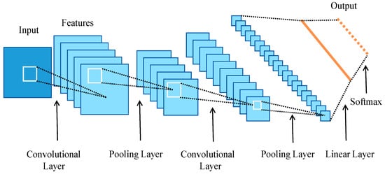
Figure 1. Structure of CNN.

The primary structure of a CNN includes the input layer, convolutional layer, pooling layer, fully connected layer, and Softmax layer. The convolutional and pooling layers serve as the core components of the CNN, usually appearing in pairs. Users can freely choose the number of convolution–pooling pairs based on the complexity of the task. This configuration can optimize the overall network structure and enhance the model’s performance [30].

Input layer: the input layer of a CNN is responsible for converting the input image or data into a 2D matrix and storing this matrix for subsequent operations [31].

Convolutional layer: The convolutional layer contains multiple convolutional kernels, which perform convolution operations on the input data to extract features. This operation calculates the convolutional kernel and the dot product of the data, assigning higher values to areas in the data with features and lower values to regions without features. The sum of these dot products is assigned to the corresponding data value in the output matrix at the current position of the convolutional kernel. By moving and calculating with the convolutional kernel repeatedly, a new matrix is obtained [32]. This paper’s suggested approach makes use of a 3 × 3 convolutional kernel. Assuming the input data are 5 × 5 and the sliding step is 1, a 3 × 3 feature map can be obtained. The convolution process is illustrated in Figure 2. The formula is listed in Equation (1).

$${\mathrm{M}}_{\mathrm{t}}=(\mathrm{m}+2\mathrm{p}-\mathrm{k})/\mathrm{s}+1,$$

(1)

where M_t denotes the feature map size, m denotes the input matrix size, k denotes the dimension of the convolutional kernel, s denotes the stride, and p denotes the number of padding layers.

Figure 2. Principle of the convolution operation, with an outline highlighting the region of the dot product.

Activation layer: The activation layer commonly consists of an activation function that introduces a nonlinear transformation to the output of the convolutional layer, giving the feature map nonlinear characteristics. Common activation functions include ReLU, tanh, and sigmoid. The model presented in this paper employs the ReLU activation function, as defined in Equation (2). ReLU offers benefits such as rapid convergence and straightforward gradient calculation [33].

$$\mathrm{ReLU}\left(\mathrm{x}\right)=\max (\mathrm{x},0),$$

(2)

Pooling layer: This is commonly positioned following the convolutional layer and serves to down-sample the extracted features, reducing the spatial dimensions and computational complexity of the data. Pooling operations commonly involve max pooling and average pooling [34]. The model proposed in this paper uses max pooling. Pooling also involves a sliding kernel, which can be referred to as a sliding window. Assume that the sliding window size is 2 × 2 and the stride is 2. At each position of the window, the maximum value within the region is chosen as the output. The pooling process is illustrated in Figure 3, and the formula is displayed in Equation (3).

$$\mathrm{X}=\mathrm{f}[\alpha \mathrm{S}(\mathrm{x})+\mathrm{b}],$$

(3)

where X represents the output of the pooling layer, f() represents the activation function, α represents the sampling coefficient, and b is the bias term.

Figure 3. Principle of the pooling process, with an outline highlighting the sliding region.

Fully connected layer: Following multiple convolution and pooling layers, the resulting feature maps are flattened row by row and then concatenated to form a vector, which is subsequently passed into a fully connected network. This layer produces the final classification result.

2.2. Temporal Convolutional Network (TCN)

The temporal convolutional network (TCN) is specifically designed for time-series data, combining various convolutional methods. It primarily employs temporal 1D convolutions and uses residual connections to mitigate issues such as vanishing and exploding gradients [35]. In terms of structure, the TCN differs from the CNN primarily in that it consists of causal convolutions, dilated convolutions, and residual connection modules. The architecture of the TCN is illustrated in Figure 4.

Figure 4. Architectural principle of TCN.

The input feature vector first undergoes dilated causal convolutions, followed by normalization using WeightNorm to accelerate model training. The ReLU activation function is then applied to introduce nonlinearity into the feature vector. Dropout is used to discard unnecessary neurons and prevent overfitting. A 1D fully convolutional layer is employed to ensure that the input sequence and output sequence of the TCN have the same length. The result is then added to the input vector to produce the final output.

Causal convolution: Causal convolution is a fundamental component of the TCN, ensuring that the network maintains causality when processing time-series data. This means that the output at any given time step depends only on the current time step and the preceding elements in the input sequence [36]. Causal convolution is achieved by adding the appropriate amount of zero padding to the left side of the input sequence, ensuring that the convolution operation does not “see” future data. Causal convolution is a key requirement for handling time-series data, as it preserves the natural temporal order. The structure of causal convolution is illustrated in Figure 5, and its formula is illustrated in Equation (4).

$${\mathrm{y}}_{\mathrm{t}}={\sum }_{\mathrm{k}=0}^{\mathrm{k}-1}{\mathrm{\omega }}_{\mathrm{k}}\cdot {\mathrm{x}}_{\mathrm{t}-\mathrm{k}},$$

(4)

where y_t denotes the output of the convolution operation, ω_k denotes the weights of the convolutional kernel, and x_t−k denotes the elements of the input sequence.

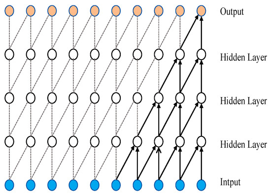
Figure 5. Principle of causal convolution.

Dilated convolution: Unlike traditional convolution, dilated convolution allows for the spaced sampling of the input during the convolution process. The sampling rate is controlled by the dilation coefficient d, as shown in the figure. For the lower layers, where d = 1, each point in the input is sampled. In the intermediate layers, where d = 2, every second point is sampled as input. Generally speaking, the value of d increases with the layer height. This indicates that as the number of layers increases, the effective receptive field’s size increases exponentially. Thus, dilated convolution enables convolutional networks to achieve large receptive fields with fewer layers [37]. The model presented in this paper uses two layers of dilated convolution. The structure of dilated convolution is depicted in Figure 6. The formula is given in Equation (5).

$${\mathrm{y}}_{\mathrm{t}}={\sum }_{\mathrm{k}=0}^{\mathrm{k}-1}{\mathrm{\omega }}_{\mathrm{k}}\cdot {\mathrm{x}}_{\mathrm{t}-\mathrm{d}\cdot \mathrm{k}},$$

(5)

where y_t denotes the output of the convolution operation, ω_k denotes the weights of the convolutional kernel, x_t−d∙k denotes the elements of the input sequence, and d denotes the dilation rate.

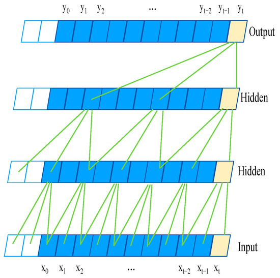
Figure 6. Principle of dilated convolution.

Residual connection: In the TCN, although the introduction of causal and dilated convolutions effectively expands the receptive field, it inevitably increases the depth of the network. This necessitates the use of residual connections to address potential issues such as gradient vanishing or gradient decay [38]. This paper takes a residual module with a convolutional kernel size of 3 and a dilation rate of 1 as an example. The structure is illustrated in Figure 7, and the formula is provided in Equation (6).

$$\mathrm{y}=\mathrm{f}(\mathrm{x}, \mathrm{p})+\mathrm{x},$$

(6)

where y denotes the output, f denotes convolution operations, p denotes the weights of the convolutional kernel, and x denotes the input.

Figure 7. Residual block of TCN.

2.3. Attention Mechanism (ATTENTION)

The core characteristic of the attention mechanism is assigning different weights to the features in the hidden layer. By adjusting the weight values, the mechanism effectively highlights key features while ignoring irrelevant information, making it easier to identify important features [39]. After extracting features through the above network layers, an attention layer is used to increase the weight of important dimensions and reduce the influence of weakly correlated dimensions on the diagnostic results. This, in turn, improves the model’s diagnostic accuracy and efficiency. Figure 6 shows the attention layer’s organizational structure. Specifically, the attention layer includes three parts: weight computation, feature weighting, and output.

In Figure 8, x is the input to the TCN, h is the output of the hidden layer obtained through the TCN, q is the weight of the hidden layer output, and y is the output. The weighted feature sequence and the attention weight matrix are the results of the attention mechanism, as shown in Equations (7)–(9).

$${\mathrm{\mu }}_{\mathrm{i}}{=\tan \mathrm{h}(\mathrm{\omega }}_{\mathrm{s}}{\mathrm{h}}_{\mathrm{t}}{+\mathrm{b}}_{\mathrm{s}})\arcsin \mathsf{\theta },$$

(7)

$${\mathrm{q}}_{\mathrm{i}}={\displaystyle \frac{{\exp (\mathrm{\mu }}_{\mathrm{i}}^{\mathrm{T}}{\mathrm{\mu }}_{\mathrm{s}})}{{\sum }_{\mathrm{i}=1}^{\mathrm{t}}{\exp (\mathrm{\mu }}_{\mathrm{i}}^{\mathrm{T}}{\mathrm{\mu }}_{\mathrm{s}})}},{\sum }_{\mathrm{i}=1}^{\mathrm{t}}{\mathrm{q}}_{\mathrm{i}}=1$$

(8)

$$\mathrm{F}={\sum }_{\mathrm{i}=1}^{\mathrm{t}}{\mathrm{q}}_{\mathrm{i}}{\mathrm{h}}_{\mathrm{t}},$$

(9)

where ω_s denotes the weight matrix, b denotes the bias term, and μ_s denotes the randomly initialized attention mechanism matrix.

Figure 8. Principle of attention.

2.4. Algorithmic Process

By integrating the strengths of different neural networks, combining a CNN and TCN is more suitable for handling fault diagnosis problems. The introduction of the attention mechanism allows for the effective selection and emphasis of key features, significantly improving diagnostic accuracy. Therefore, a combined diagnostic model based on CNN-TCN–ATTENTION is proposed for diesel engine fault diagnosis. One-dimensional thermodynamic data are used as input. After convolution, pooling, and activation operations, the signal’s deep characteristics are subsequently supplied to the TCN residual module. The attention mechanism calculates the attention weight vector based on the current input vector and combines it with the extracted features to generate a new feature vector. The fully connected layer then receives this feature vector as input. The characteristics of this model are shown in Table 2. Figure 9 is the algorithm structure of the CNN-TCN–ATTENTION fault diagnosis model. Figure 10 is the algorithm flowchart.

Table 2. The performance characteristics of CNN-TCN–ATTENTION.

Advantages	Disadvantages
Strong feature extraction	High parameter count
Excellent temporal modeling	Slow training time
High robustness	Data dependency
Strong transferability	Limited interpretability

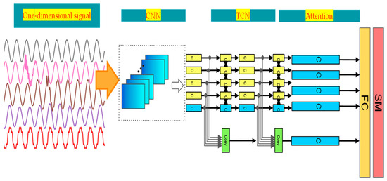
Figure 9. Structure of CNN-TCN–ATTENTION.

Figure 10. Flowchart of CNN-TCN–ATTENTION.

3. Experiment

3.1. Experimental Data

3.1.1. Diesel Engine Simulation Model and Fault Simulation

This paper takes the Wärtsilä W6X72DF marine diesel engine as the object for fault diagnosis. Due to the high cost, potential hazards, and destructiveness of simulating faults in actual ship operation, obtaining fault data is challenging. Therefore, this paper adopts a modeling and simulation approach to mathematically model the W6X72DF marine diesel engine. The simulation results are compared with actual test data to validate the model’s accuracy. The modeling software used is the engine simulation software GT-Power (Version 2020). The diesel engine simulation model is illustrated in Figure 11.

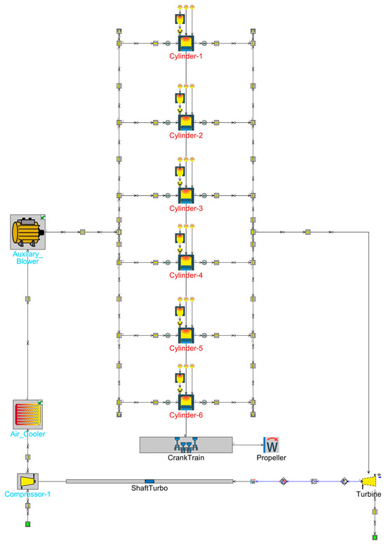
Figure 11. W6X72DF simulation model.

To validate the dependability of the diesel engine simulation model, this paper selects the engine running under the 100% load condition in gas mode as the research object. The simulation model results are compared with the engine manufacturer’s test data, with the comparison displayed in Table 3.

Table 3. Comparison of simulation model parameters and test data parameters.

Parameter	Running Value	Simulation Value	Error/%
Engine speed [RPM]	69.1	69.27	0.25
Brake power [kW]	13,265	13,394.27	0.97
BSEC—pilot fuel [kJ/kW·h]	13.4	13.39	−0.93
BSEC—natural gas [kJ/kW·h]	6685.6	6621.42	−0.96
Peak pressure [bar]	172.3	170.68	−0.94
Post-compressor pressure [bar]	4.03	3.98	−1.24
Post-compressor temperature [K]	476	488.26	2.58
Pre-turbine temperature [K]	660	651.05	−1.36
Post-turbine temperature [K]	486	488.13	0.44
Pre-turbine pressure [bar]	3.9	3.81	−2.31
Boost Pressure [bar]	3.98	3.97	−0.25

According to Table 4, the error between the simulation model and the actual diesel engine test data is controlled within 3%, which satisfies the fault simulation requirements. In this paper, four types of faults are simulated: normal operating condition (F0), air compressor fault (F1), intercooler fault (F2), single-cylinder gas flow reduction (F3), and turbine fault (F4). The specific fault scenarios are presented in Table 4.

Table 4. Fault simulation scenarios.

Fault Type	Fault Feature Parameter	Normal Value	Fault Severity Level
			LV1	LV2	LV3	LV4
F1	Air compressor efficiency/%	100	95	90	85	80
F2	Intercooler efficiency/%	100	95	90	85	80
F3	Gas capacity per cylinder/g	71.3	67.74	64.17	60.61	57.04
F4	Turbine failure/%	100	95	90	85	80

3.1.2. Data Acquisition and Preprocessing

In this paper, the fault parameter for the diagnostic model is chosen from the thermodynamic parameters produced during diesel engine operation. To provide a comprehensive display of how various faults affect the engine’s performance, 22 thermodynamic parameters are chosen as fault data. These include the following: speed (N), maximum pressure (Pz), effective torque (T), intake air flow (F), effective power (Pe), indicated power (Pi), Indicated Mean Effective Pressure (IMEP), Brake Mean Effective Pressure (BMEP), Indicated Specific Fuel Consumption (ISFC), Brake Specific Fuel Consumption (BSFC), turbocharger outlet pressure (Pmp1) and temperature (Tmp1), intercooler outlet pressure (Pmp2) and temperature (Tmp2), cylinder intake pressure (Pmp3) and temperature (Tmp3), cylinder exhaust pressure (Pmp4) and temperature (Tmp4), turbine inlet pressure (Pmp5) and temperature (Tmp5), and turbine outlet pressure (Pmp6) and temperature (Tmp6). In the GT-Power software (Version 2020), the diesel engine model is set with the four faults listed in Table 2. Fault values are taken every 0.87 s (one cycle time), and for each fault, 360 sets of data are collected with a duration of 313.2 s. Similarly, data are collected for the normal state with the corresponding number of cycles. This results in a total of 1800 sets of 22-dimensional data, with 1440 sets of fault data and 360 sets of normal data. A part of the operation data is shown in Table 5.

Table 5. Thermodynamic parameter data for diesel engine under different states.

Parameter	Parameter Values for 5 Running States
	F0	F1	F2	F3	F4
N (r/min)	69.27	68.25	68.01	68.26	68.26
Pz (bar)	172.3	151.98	153.42	155.92	151.89
T (N-m)	1,850,111.60	1,791,066.60	1,778,327.60	1,792,177.60	1,791,566.60
F (g/s)	5028.95	3822.88	3960.63	5042.83	3816.25
Pi (Kw)	13,696.50	13,058.63	12,921.95	13,067.69	13,064.00
Pe (Kw)	13,435.14	12,801.39	12,665.61	12,810.43	12,806.73
IMEP (bar)	15.72	15.23	15.12	15.24	15.23
BMEP (bar)	15.42	14.93	14.82	14.94	14.93
ISFC (g/Kwh)	140.32	144.85	145.87	140.30	144.81
BSFC (g/Kwh)	143.05	147.76	148.82	143.11	147.72
Pmp1 (bar)	4.03	3.27	3.43	3.93	3.27
Tmp1 (K)	476	491.54	500	483.41	455.68
Pmp2 (bar)	4.04	3.27	3.43	3.93	3.26
Tmp2 (K)	313.65	315.39	352.34	313.56	313.82
Pmp3 (bar)	3.58	3.03	3.03	3.51	3.03
Tmp3 (K)	312.87	314.53	349.28	312.68	313.05
Pmp4 (bar)	3.43	2.73	2.83	3.33	2.74
Tmp4 (K)	624.76	701.47	718.37	569.44	700.86
Pmp5 (bar)	3.9	3.16	3.29	3.76	3.15
Tmp5 (K)	660	743.35	757.01	643.49	742.74
Pmp6 (bar)	1.01	1.01	1.01	1.01	1.01
Tmp6 (K)	486	580.90	586.59	483.02	612.89

To confirm that the simulated defects are effective, a qualitative analysis is conducted by comparing the deviation rate of fault data at different fault severities against the thermodynamic parameters under normal conditions. The qualitative analysis is shown in Figure 12. The fault simulation results align with the expert experience analysis, verifying the accuracy and reasonableness of the fault simulation data. The formula for the qualitative analysis is presented in Equation (10).

$${\mathsf{\Delta }=(\mathrm{x}}_{\mathrm{i}}-\mathrm{x})/\mathrm{x}\cdot 100\%,$$

(10)

where x_i denotes the thermodynamic parameter value under a specific fault condition, and x denotes the thermodynamic parameter value under normal operating conditions.

Figure 12. Deviation rates of diesel engine parameters at different fault severities.

Due to the different dimensions of the thermal parameter data in marine diesel engines, there is a significant discrepancy in the magnitude of the data, which may affect the training procedure. Hence, the data should be normalized prior to training. In this study, the min-max normalization method is selected. The advantage of this method is that it normalizes the data without altering the data distribution [40]. The calculation formula is presented in Equation (11).

$${\mathrm{x}}^{*}={\displaystyle \frac{\mathrm{x} - \min \left(\mathrm{x}\right)}{\max \left(\mathrm{x}\right) - \min \left(\mathrm{x}\right)}},$$

(11)

where min(x) and max(x) denote the maximum and minimum values of x, respectively.

3.2. Experimental Evaluation Criterion

The evaluation of the model’s fault diagnosis performance needs to consider multiple perspectives and integrate various factors. For the fault diagnosis model, the accuracy, precision, recall, and F1 score are used as evaluation metrics in this paper, as they can comprehensively reflect the model’s overall performance; these metrics provide a thorough evaluation of the model’s performance by assessing the precision and recall balance, the accuracy of positive class predictions, and the capacity to detect all positive samples. The formulas for the F1 score, recall, accuracy, and precision are provided in Equation (12):

$$\begin{gathered} \mathrm{Accuracy}={\displaystyle \frac{\mathrm{TP}+\mathrm{TN}}{\mathrm{TP}+\mathrm{FP}+\mathrm{TN}+\mathrm{FN}}} \\ \mathrm{Precision}={\displaystyle \frac{\mathrm{TP}}{\mathrm{TP}+\mathrm{FP}}} \\ \mathrm{Recall}={\displaystyle \frac{\mathrm{TP}}{\mathrm{TP}+\mathrm{FN}}} \\ \mathrm{F}1={\displaystyle \frac{2\times \mathrm{TP}}{2\times \mathrm{TP}+\mathrm{FP}+\mathrm{FN}}} \end{gathered}$$

(12)

In this context, TP denotes a true positive, FP denotes a false positive, TN denotes a true negative, and FN denotes a false negative.

3.3. Ablation Experiment

The proposed model in this paper is accomplished in PyTorch 1.12.0+cu113 and Python 3.9, with the GPU configuration being an NVIDIA GeForce RTX 1080 Ti. The model uses the data collected from the aforementioned engine simulation model as the experimental dataset, which consists of 1800 sets of 22-dimensional data. These are divided into 4 types of fault samples and 1 type of normal sample, with each type containing 360 sets of data. The data are split into training, test, and validation sets in a 7:2:1 ratio, i.e., 1260 sets of data for training, 360 sets for testing, and 180 sets for validation. The model is trained on the engine dataset and evaluated using the train/val split method and trained by minimizing the cross-entropy loss function, which, for multi-class tasks, can be expressed as Equation (13). After each epoch, the model’s performance is assessed using the validation set, and the best model is saved. Once training is complete, the best model is loaded, and its final performance is evaluated on an independent test set. The confusion matrix and classification report of the test set are calculated.

$$\mathrm{Loss}=-{\sum }_{\mathrm{i}}{\sum }_{\mathrm{c}=1}^{\mathrm{M}}{\mathrm{y}}_{\mathrm{ic}}{\log (\mathrm{p}}_{\mathrm{ic}}),$$

(13)

In this context, M denotes the number of classes; the indicator function y_ic is 1 if the true class of sample i is c and 0 otherwise. The predicted probability of sample i belonging to class c is represented as p_ic.

The model’s hyperparameters were determined through multiple independent experiments, following common deep learning practices and previous research. The initial learning rate was set to 0.0003, and the Adam optimizer, which combines the Momentum and RMSprop gradient descent methods, was used to optimize the model parameters and learning rate. This optimizer has been proven to be effective for various neural networks. The batch size for the training set was set to 32, with a dropout rate of 0.5 and the ReLU activation function. The model was trained for 100 epochs. The detailed configuration of the CNN-TCN–ATTENTION model is presented in Table 6.

Table 6. Details of CNN-TCN–ATTENTION.

Layers	Description	Details
1	Input	input_shape = (32,1,22)
2	Conv	Filters = 32, kernel_size = 3, strides = 1, padding = 1, activation = ReLu
3	Max pooling	Kernel_size = 2, strides = 2, padding = 0
4	Conv1	Filters = 16, kernel_size = 3, strides = 1, padding = 1, dropout = 0.5, activation = ReLu
5	Conv2	Filters = 16, kernel_size = 3, strides = 1, padding = 1, dropout = 0.5, activation = ReLu
6	Conv1d	Filters = 16, kernel_size = 3, strides = 1, padding = 1, activation = ReLu
7	Attention	(Query, Key, Value), filters = 16, activation = linear
8	FC	layer_size = 160, activation = linear
9	FC	layer_size = 5, activation = linear

3.3.1. Ablation Experiment of Convolution Layer

Ablation experiments are conducted to select the appropriate network structure by evaluating the number of convolution–pooling pairs, thereby avoiding issues such as overfitting due to excessive layers, reduced efficiency, and higher costs associated with a more complex structure. Multiple experiments are performed on the number of layers in the CNN and TCN, and the average results are taken to calculate the performance of the network models with different layer counts. The results are displayed in Table 7, and the accuracy and loss curves for the training and validation sets are depicted in Figure 13.

Table 7. Experimental results with different numbers of convolution layers.

Model	CNN Conv	TCN Conv	Test Accuracy/%	Running Time/s	Trainable Parameters
A	1	1	95.63	23	3100
B	1	2	100	29	3900
C	2	1	99.43	30	4574
D	2	2	99.72	33	5374

Figure 13. Training and validation accuracy and loss rates for different numbers of convolution layers.

From Table 7 and Figure 13, it can be observed that Model A has a lower accuracy in the test set, and its loss curve converges poorly. Even after the accuracy starts to converge, the loss curve continues to decrease. This is due to the relatively small number of convolutional layers in the CNN and TCN, which causes fluctuations in the network’s stability and insufficient feature extraction capabilities of local structures. Moreover, Model A has 3100 trainable parameters and a training time of 23 s, which is advantageous compared to the other three models. However, due to its simpler network structure, its performance in terms of accuracy and convergence is suboptimal, leading to unsatisfactory diagnostic results. In contrast, Model C and Model D show higher accuracies in the test set, 99.43% and 99.72%, respectively. However, when compared to Model B, it is evident that as the number of convolution layers increases, the accuracy begins to decline. This is because an excessive number of layers leads to model overfitting due to the complexity of the network structure. Additionally, the training time increases to 30s and 33s, and the convergence rate is slower than that of Model B. Occasional small gradient explosion phenomena also occur during training. Gradient explosion is a common issue in deep learning, which can destabilize the network. Model C has 4574 trainable parameters, and Model D has 5374, which makes them more complex than the other models. Thus, both Model C and Model D are not ideal choices overall. When selecting Model B, it achieves the highest accuracy in the test set, reaching 100%. The number of trainable parameters in Model B is 3900, which is slightly more than Model A but more balanced compared to Models C and D. Moreover, its training time is shorter, making it the most efficient model overall. Therefore, Model B’s architecture is chosen as the foundation for the combined model, and the subsequent research is based on this model.

3.3.2. Ablation Experiment of Network Structure

The purpose of this experiment is to validate the contribution of each network unit in the proposed model to the overall performance, thereby proving its reliability. For the network structure ablation study, the model details and hyperparameter settings are as introduced at the beginning of this section. Under unchanged conditions, ablation experiments are performed on the CNN, TCN, ATTENTION, and combined models. Each model undergoes multiple trials to obtain the evaluation results for the test set. The final experimental results are presented in Table 8.

Table 8. Diagnostic accuracy of different diagnosis models.

Diagnostic Model	Test Accuracy/%	Precision/%	Recall/%	F1 Score/%	Running Time/s
CNN	90.62	92.92	89.66	89.14	15
TCN	89.38	89.98	89.89	89.91	20
CNN-TCN	91.87	95	91.03	91.37	21
CNN-TCN–ATTENTION	100	100	100	100	29

As shown in Table 8, when a CNN or TCN is used individually, although the structure is simple and the computational complexity is low, the diagnostic accuracy is relatively low. This is because each model focuses only on features that match its respective extraction characteristics and is not sensitive to other types of features, leading to poor performance when used alone. When the CNN and TCN are combined, the model complexity becomes moderate, and the feature extraction is more comprehensive. However, compared to the individual CNN or TCN models, the diagnostic accuracy does not improve significantly. This is because the features extracted by the CNN and TCN are heterogeneous, making feature fusion difficult, and there is a lack of focus on key information, which results in no significant improvement in the model’s diagnostic performance. To address the feature fusion problem, the attention mechanism is introduced to integrate the features extracted by both the CNN and TCN, rationally allocate feature weights, and thus optimize the model. As a result, the model achieves optimal accuracy, reaching 100% in the test set. The confusion matrices for the different models are shown in Figure 14. In Figure 14, the dark blue blocks represent correctly diagnosed fault samples in the test set, while the light blue blocks represent misdiagnosed fault samples. From the confusion matrix, it can be seen that the combined model accurately classifies each fault category, achieving 100% accuracy, outperforming the other ablation models. It is worth noting that the confusion matrix for the CNN clearly shows that its recognition of Category 3 is significantly weaker compared to the other three models. This is because the time-series features of Fault 3 are relatively stable, and the CNN’s sensitivity to such features is insufficient. In contrast, the other three models, after introducing the TCN, show improved classification accuracy for Category 3, which highlights the role of the TCN unit in this model. At the same time, this experiment also validates the functionality of each component in the combined model mentioned earlier. Specifically, the CNN extracts local spatial features, the TCN captures temporal features, and ATTENTION integrates the features and assigns different weights to the features, thereby improving the classification accuracy of the model.

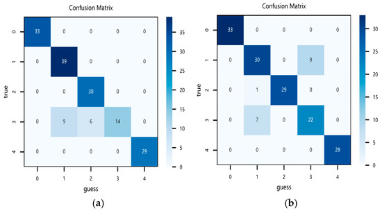
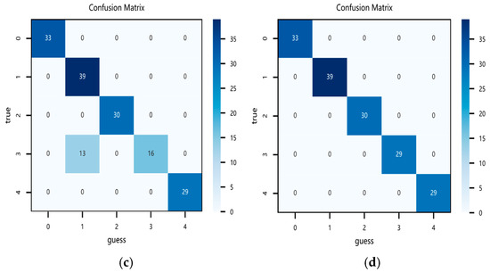
Figure 14. Confusion matrices of different models: (a) CNN, (b) TCN, (c) CNN-TCN, and (d) CNN-TCN–ATTENTION.

3.4. Noise Experiment

The sensor data of marine diesel engines are often influenced by various factors, such as environmental conditions and the operating status of the equipment, and are accompanied by various types of noise. To make the research method more representative of the actual working conditions of the diesel engine, noise can be introduced into the fault data to simulate the real data collected by sensors.

To evaluate the performance of the CNN-TCN–ATTENTION diagnostic model under noisy conditions, random noise with an intensity of 10%, Gaussian noise with a signal-to-noise ratio (SNR) of 15, and salt-and-pepper noise with a noise density of 0.05 are added to the marine diesel engine dataset. The diagnostic accuracy of each model under these three noise conditions is calculated. The experimental environment and parameter settings remain the same as those introduced at the beginning of this section. The diagnostic accuracy in the test set under these conditions is shown in Table 9, and the results are illustrated in Figure 15.

Table 9. Diagnostic accuracy under different noise conditions.

Diagnostic Model	Noise Class	Test Accuracy
CNN-TCN–ATTENTION	Noiseless	100%
	Random noise	98.75%
	Gaussian noise	97.5%
	Impulse noise	94.37%
CNN-TCN	Noiseless	91.87%
	Random noise	82.5%
	Gaussian noise	76.25%
	Impulse noise	78.12%
TCN	Noiseless	89.38%
	Random noise	78.12%
	Gaussian noise	77.5%
	Impulse noise	75.62%
CNN	Noiseless	90.62%
	Random noise	72.5%
	Gaussian noise	73.12%
	Impulse noise	70%

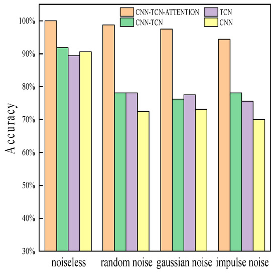
Figure 15. Test accuracy under different noise conditions.

As shown in Figure 15, different types of noise have a certain degree of impact on the accuracy of each network model in the test set. Specifically, the accuracy of all models exhibits a downward trend. However, the CNN-TCN–ATTENTION model experiences the least decrease, with its diagnostic accuracy remaining above 90%. This demonstrates the model’s strong noise resistance while maintaining highly favorable precision. This can be attributed to the ability of the CNN to extract local features, the ability of the TCN to process time-series data, and the focusing effect of the attention mechanism on key information when noise is present at various levels and in different features. These factors make the model resilient to noise, enabling it to filter out irrelevant information and enhance robustness. This confirms that the model possesses high robustness under various noise conditions, making it suitable for marine diesel engine fault diagnosis.

3.5. Contrast Experiment

To further validate the performance of the CNN-TCN–ATTENTION model, four popular deep learning models, namely Transformer, GRU, LSTM, and DBN, are selected for comparison. The dataset is input into each of the four comparison models, and to minimize randomness, each model is run 10 times, with the average result taken. The results are shown in Table 10, and the evaluation results for each model are presented in Figure 16. The experimental results indicate that the CNN-TCN–ATTENTION model achieves state-of-the-art performance in marine diesel engine fault diagnosis tasks. Although the LSTM and Transformer models achieve accuracy rates exceeding 90% in the test set and have shorter runtimes, there remains a noticeable performance gap compared to the CNN-TCN–ATTENTION model. Furthermore, the GRU and DBN exhibit unsatisfactory accuracy in the test set. Overall, the CNN-TCN–ATTENTION model demonstrates significant advantages.

Table 10. Comparison of diagnostic accuracy across different models.

Algorithms	Test Accuracy %	Running Time/s
CNN-TCN–ATTENTION	100	29
Transformer	90.62	22
LSTM	93.13	23
GRU	83	19
DBN	84.4	20

Figure 16. Confusion matrices of different models: (a) Transformer model, (b) LSTM model, (c) GRU model, and (d) DBN model.

To highlight the specific classification performance of different diagnostic algorithms for faults, in addition to the aforementioned accuracy and runtime, this study also analyzes the precision and recall of each diagnostic algorithm. The results are presented in Table 11.

Table 11. Precision and recall for each algorithm.

Algorithms	Precision					Recall
	F0	F1	F2	F3	F4	F0	F1	F2	F3	F4
CNN-TCN–ATTENTION	1	1	1	1	1	1	1	1	1	1
Transformer	1	0.81	0.83	1	1	1	1	1	0.48	1
LSTM	1	0.78	1	1	1	1	1	1	0.62	1
GRU	1	0.68	1	0.76	1	1	0.57	1	1	1
DBN	1	1	1	1	1	1	0.22	1	1	1

As shown in Table 11, most algorithms can accurately classify normal operating conditions. However, the complexity of engine fault data leads to relatively poor classification performance for the GRU and DBN, which are less sensitive to temporal features. Although Transformer and LSTM achieve higher precision for each fault category compared to the GRU and DBN, their recall rates for condition F3 are relatively low. Furthermore, the precision of Transformer and LSTM in conditions F1 and F2 is lower than that of the proposed CNN-TCN–ATTENTION model. The CNN-TCN–ATTENTION model achieves 100% accuracy and recall across all conditions, demonstrating a significant advantage over the other diagnostic algorithms and better aligning with practical industrial requirements.

As shown in Figure 16, the four comparison algorithms exhibit varying degrees of misclassification under conditions F1, F2, F3, and F4. In contrast, the confusion matrix in Figure 14d illustrates that the proposed CNN-TCN–ATTENTION model achieves complete recognition for each fault type. This indicates that the CNN-TCN–ATTENTION model can extract more information from the data, thereby enhancing the classification accuracy and stability of the diagnostic algorithm, outperforming the other models.

The experimental data show that the CNN-TCN–ATTENTION model achieves excellent results in the marine diesel engine fault diagnosis task. Specifically, as shown in Figure 16, the LSTM model, which is currently the most widely used, has the highest accuracy (93.13%) out of the four models used for comparison. However, its performance in the validation set is poor, with significant fluctuations in the accuracy curve, indicating its instability. The other three models exhibit poor convergence of the loss rate curve and lower accuracy, which can also be seen in the confusion matrices in Figure 16. Compared to the confusion matrix of the combined model in Figure 14, the comparison models show more light blue blocks, indicating a higher number of misdiagnosed samples and thus lower accuracy. Furthermore, compared to traditional algorithms, CNN-TCN–ATTENTION shows faster convergence, and the model evaluation results demonstrate that it effectively identifies fault types in marine diesel engines.

The Transformer model is sensitive to positional information and requires additional positional encoding to provide sequence information to improve accuracy. LSTM has strong feature extraction capabilities but tends to lose the correlation between channels, which can lead to overfitting. The GRU model has a simpler structure and, like LSTM, experiences overfitting issues when training data are limited or the model has many parameters. The DBN has a complex structure and training algorithm, involving numerous parameters, and improper parameter selection may cause learning to converge to a local optimum, negatively impacting model performance. On the other hand, the CNN model is simple, with flexible layers and powerful global feature extraction capabilities, while the TCN is effective in capturing temporal dependencies and sequence patterns and is less prone to overfitting than the RNN and its variants. The CNN-TCN–ATTENTION model combines the advantages of both the CNN and TCN, utilizing the attention mechanism to highlight significant features that increase model accuracy while extracting features at various scales. This suggests that the CNN-TCN is effective at feature extraction, and the attention mechanism further enhances model accuracy. Thus, compared to more conventional models, the CNN-TCN–ATTENTION model is more reliable, accurate, and efficient in identifying problems in marine diesel engines.

4. Conclusions

This paper addresses the current challenges in marine diesel engine fault diagnosis, such as insufficient accuracy and inadequate feature extraction, by introducing the CNN-TCN–ATTENTION model. This novel intelligent fault diagnosis approach for marine engines combines deep learning techniques. The conclusion of the approach applied in this paper is as follows:

• Given the difficulty of obtaining fault data for marine diesel engines, a modeling and simulation approach is employed to extract fault data that meet the requirements of fault diagnosis.
• The combination of a CNN and TCN for feature extraction is applied for the first time in the field of marine diesel engine fault diagnosis to improve feature extraction capabilities. This approach first uses the CNN to extract global features, followed by the TCN to capture temporal sequence features. Additionally, an attention mechanism is introduced to address the issue of insufficient feature fusion. This mechanism effectively assigns different weights to important features, thereby achieving feature fusion and improving the model’s accuracy.
• To validate the effectiveness of the CNN-TCN–ATTENTION model, three different experimental cases were carefully designed. Specifically, in the ablation experiment, the quantity of convolution layers in the CNN network was adjusted through a controlled variable method to find the optimal layer distribution scheme. Additionally, by removing each component of the model, the accuracy of the CNN-TCN–ATTENTION model achieved 100%, outperforming the other ablation models. In the noise experiment, different types of noise were added to observe the model’s accuracy trend, demonstrating the robustness of the proposed model. In the comparative experiment, the CNN-TCN–ATTENTION model was compared with other deep learning models, and the CNN-TCN–ATTENTION model surpassed all other models in accuracy, confirming the suggested method’s efficacy.

In conclusion, the approach suggested in this paper demonstrates significant advantages in addressing the challenge of insufficient feature extraction in marine diesel engine fault diagnosis by combining feature extraction models. This work provides valuable theoretical insights for the advancement of fault diagnosis in marine diesel engines.

Moreover, in practical applications, annotated fault datasets are often scarce, and it is challenging and expensive to manually label a large number of defect samples. Therefore, we plan to enhance the CNN-TCN–ATTENTION model with feature-based transfer learning methods to apply it to other fault diagnosis tasks with limited labeled data [41,42]. By aligning the characteristics of the target and source domains in a shared area, the model will learn domain-invariant features, ultimately improving its adaptability.

References

- Gharib, H.; Kovács, G. A Review of Prognostic and Health Management (PHM) Methods and Limitations for Marine Diesel Engines: New Research Directions. Machines 2023, 11, 695. [Google Scholar] [CrossRef]
- Orhan, M.; Celik, M. A literature review and future research agenda on fault detection and diagnosis studies in marine machinery systems. Proc. Inst. Mech. Eng. Part M J. Eng. Marit. Environ. 2023, 238, 147509022211492. [Google Scholar] [CrossRef]
- Lv, Y.; Yang, X.; Li, Y.; Liu, J.; Li, S. Fault detection and diagnosis of marine diesel engines: A systematic review. Ocean Eng. 2024, 294, 116798. [Google Scholar] [CrossRef]
- Velasco-Gallego, C.; Lazakis, I. RADIS: A real-time anomaly detection intelligent system for fault diagnosis of marine machinery. Expert Syst. Appl. 2022, 204, 117634. [Google Scholar] [CrossRef]
- Ahn, Y.-G.; Kim, T.; Kim, B.-R.; Lee, M.-K. A Study on the Development Priority of Smart Shipping Items—Focusing on the Expert Survey. Sustainability 2022, 14, 6892. [Google Scholar] [CrossRef]
- Hu, X.X.; Tang, T.; Tan, L.; Zhang, H. Fault Detection for Point Machines: A Review, Challenges, and Perspectives. Actuators 2023, 12, 391. [Google Scholar] [CrossRef]
- Zhou, Y.; Wang, Z.; Zuo, X.; Zhao, H. Identification of wear mechanisms of main bearings of marine diesel engine using recurrence plot based on CNN model. Wear 2023, 520–521, 204656. [Google Scholar] [CrossRef]
- Shahid, S.M.; Ko, S.; Kwon, S. Real-time abnormality detection and classification in diesel engine operations with convolutional neural network. Expert Syst. Appl. 2022, 192, 116233. [Google Scholar] [CrossRef]
- Chen, S.; Ge, H.; Li, J.; Pecht, M. Progressive Improved Convolutional Neural Network for Avionics Fault Diagnosis. IEEE Access 2019, 7, 177362–177375. [Google Scholar] [CrossRef]
- Qin, C.; Jin, Y.; Zhang, Z.; Yu, H.; Tao, J.; Sun, H.; Liu, C. Anti-noise diesel engine misfire diagnosis using a multi-scale CNN-LSTM neural network with denoising module. CAAI Trans. Intell. Technol. 2023, 8, 963–986. [Google Scholar] [CrossRef]
- Zhao, H.; Mao, Z.; Zhang, J.; Zhang, X.; Zhao, N.; Jiang, Z. Multi-branch convolutional neural networks with integrated cross-entropy for fault diagnosis in diesel engines. Meas. Sci. Technol. 2021, 32, 045103. [Google Scholar] [CrossRef]
- Dao, F.; Zeng, Y.; Qian, J. Fault diagnosis of hydro-turbine via the incorporation of bayesian algorithm optimized CNN-LSTM neural network. Energy 2024, 290, 130326. [Google Scholar] [CrossRef]
- Wang, Z.Z.; Dong, Y.J.; Liu, W.; Ma, Z. A Novel Fault Diagnosis Approach for Chillers Based on 1-D Convolutional Neural Network and Gated Recurrent Unit. Sensors 2020, 20, 2458. [Google Scholar] [CrossRef]
- Darvishi, H.; Ciuonzo, D.; Rossi, P.S. Deep Recurrent Graph Convolutional Architecture for Sensor Fault Detection, Isolation, and Accommodation in Digital Twins. IEEE Sens. J. 2023, 23, 29877–29891. [Google Scholar] [CrossRef]
- Fravolini, M.L.; del Core, G.; Papa, U.; Valigi, P.; Napolitano, M.R. Data-Driven Schemes for Robust Fault Detection of Air Data System Sensors. IEEE Trans. Control. Syst. Technol. 2019, 27, 234–248. [Google Scholar] [CrossRef]
- Kumar, A.; Parey, A.; Kankar, P.K. A New Hybrid LSTM-GRU Model for Fault Diagnosis of Polymer Gears Using Vibration Signals. J. Vib. Eng. Technol. 2024, 12, 2729–2741. [Google Scholar] [CrossRef]
- Sun, W.J.; Yan, R.Q.; Jin, R.B.; Xu, J.W.; Yang, Y.; Chen, Z.H. LiteFormer: A Lightweight and Efficient Transformer for Rotating Machine Fault Diagnosis. IEEE Trans. Reliab. 2024, 73, 1258–1269. [Google Scholar] [CrossRef]
- Tang, J.; Zheng, G.H.; Wei, C.; Huang, W.B.; Ding, X.X. Signal-Transformer: A Robust and Interpretable Method for Rotating Machinery Intelligent Fault Diagnosis Under Variable Operating Conditions. IEEE Trans. Instrum. Meas. 2022, 71, 3511911. [Google Scholar] [CrossRef]
- Zhao, D.Z.; Wang, T.Y.; Chu, F.L. Deep convolutional neural network based planet bearing fault classification. Comput. Ind. 2019, 107, 59–66. [Google Scholar] [CrossRef]
- Nauta, M.; Bucur, D.; Seifert, C. Causal Discovery with Attention-Based Convolutional Neural Networks. Mach. Learn. Knowl. Extr. 2019, 1, 312–340. [Google Scholar] [CrossRef]
- Rethage, D.; Pons, J.; Serra, X. A Wavenet for Speech Denoising. In Proceedings of the 2018 IEEE International Conference on Acoustics, Speech and Signal Processing (ICASSP), Calgary, AB, Canada, 15–20 April 2018; pp. 5069–5073. [Google Scholar]
- Yin, H.C.; Xu, H.T.; Zhang, H.; Wang, J.; Fang, X. MC-ABDS: A system for low SNR fault diagnosis in industrial production with intense overlapping and interference. Appl. Acoust. 2025, 227, 110217. [Google Scholar] [CrossRef]
- Zhang, Y.Z.; Zhao, X.Q. Remaining useful life prediction of bearings based on temporal convolutional networks with residual separable blocks. J. Braz. Soc. Mech. Sci. Eng. 2022, 44, 527. [Google Scholar] [CrossRef]
- E, G.; Gao, H.; Lu, Y.; Zheng, X.; Ding, X.; Yang, Y. A Novel Attention Temporal Convolutional Network for Transmission Line Fault Diagnosis via Comprehensive Feature Extraction. Energies 2023, 16, 7105. [Google Scholar] [CrossRef]
- Tong, A.S.; Zhang, J.; Xie, L.Y. Intelligent Fault Diagnosis of Rolling Bearing Based on Gramian Angular Difference Field and Improved Dual Attention Residual Network. Sensors 2024, 24, 2156. [Google Scholar] [CrossRef]
- Zhao, D.Z.; Shao, D.P.; Cui, L.L. CTNet: A data-driven time-frequency technique for wind turbines fault diagnosis under time-varying speeds. ISA Trans. 2024, 154, 335–351. [Google Scholar] [CrossRef]
- Yang, X.; Bi, F.; Cheng, J.; Tang, D.; Shen, P.; Bi, X. A Multiple Attention Convolutional Neural Networks for Diesel Engine Fault Diagnosis. Sensors 2024, 24, 2708. [Google Scholar] [CrossRef] [PubMed]
- Brauwers, G.; Frasincar, F. A General Survey on Attention Mechanisms in Deep Learning. IEEE Trans. Knowl. Data Eng. 2023, 35, 3279–3298. [Google Scholar] [CrossRef]
- Li, Z.; Liu, F.; Yang, W.; Peng, S.; Zhou, J. A Survey of Convolutional Neural Networks: Analysis, Applications, and Prospects. IEEE Trans. Neural Netw. Learn. Syst. 2022, 33, 6999–7019. [Google Scholar] [CrossRef] [PubMed]
- Schmidhuber, J. Deep learning in neural networks: An overview. Neural Netw. 2015, 61, 85–117. [Google Scholar] [CrossRef] [PubMed]
- Su, Y.; Gan, H.; Ji, Z. Research on Multi-Parameter Fault Early Warning for Marine Diesel Engine Based on PCA-CNN-BiLSTM. J. Mar. Sci. Eng. 2024, 12, 965. [Google Scholar] [CrossRef]
- Gao, L.; Chen, P.-Y.; Yu, S. Demonstration of Convolution Kernel Operation on Resistive Cross-Point Array. IEEE Electron Device Lett. 2016, 37, 870–873. [Google Scholar] [CrossRef]
- Xu, Y.S.; Zhang, H.Z. Convergence of deep ReLU networks. Neurocomputing 2024, 571, 127174. [Google Scholar] [CrossRef]
- Khan, A.; Sohail, A.; Zahoora, U.; Qureshi, A.S. A survey of the recent architectures of deep convolutional neural networks. Artif. Intell. Rev. 2020, 53, 5455–5516. [Google Scholar] [CrossRef]
- Fan, J.; Zhang, K.; Huang, Y.; Zhu, Y.; Chen, B. Parallel spatio-temporal attention-based TCN for multivariate time series prediction. Neural Comput. Appl. 2021, 35, 13109–13118. [Google Scholar] [CrossRef]
- Lopes, I.O.; Zou, D.Q.; Abdulqadder, I.H.; Akbar, S.; Li, Z.; Ruambo, F.; Pereira, W. Network intrusion detection based on the temporal convolutional model. Comput. Secur. 2023, 135, 103465. [Google Scholar] [CrossRef]
- Chen, Y.T.; Kang, Y.F.; Chen, Y.X.; Wang, Z.Z. Probabilistic forecasting with temporal convolutional neural network. Neurocomputing 2020, 399, 491–501. [Google Scholar] [CrossRef]
- Shafiq, M.; Gu, Z. Deep Residual Learning for Image Recognition: A Survey. Appl. Sci. 2022, 12, 8972. [Google Scholar] [CrossRef]
- Chaudhari, S.; Mithal, V.; Polatkan, G.; Ramanath, R. An Attentive Survey of Attention Models. ACM Trans. Intell. Syst. Technol. 2021, 12, 53. [Google Scholar] [CrossRef]
- Gajera, V.; Shubham; Gupta, R.; Jana, P.K. An Effective Multi-Objective Task Scheduling Algorithm using Min-Max Normalization in Cloud Computing. In Proceedings of the 2016 2nd International Conference on Applied and Theoretical Computing and Communication Technology (ICATCCT), Bangalore, India, 21–23 July 2016; pp. 812–816. [Google Scholar]
- Guo, Y.; Zhang, J. Fault Diagnosis of Marine Diesel Engines under Partial Set and Cross Working Conditions Based on Transfer Learning. J. Mar. Sci. Eng. 2023, 11, 1527. [Google Scholar] [CrossRef]
- Wang, L.; Cao, H.; Cui, Z.; Ai, Z. A Fault Diagnosis Method for Marine Engine Cross Working Conditions Based on Transfer Learning. J. Mar. Sci. Eng. 2024, 12, 270. [Google Scholar] [CrossRef]
Disclaimer/Publisher’s Note: The statements, opinions and data contained in all publications are solely those of the individual author(s) and contributor(s) and not of MDPI and/or the editor(s). MDPI and/or the editor(s) disclaim responsibility for any injury to people or property resulting from any ideas, methods, instructions or products referred to in the content. |
© 2025 by the authors. Licensee MDPI, Basel, Switzerland. This article is an open access article distributed under the terms and conditions of the Creative Commons Attribution (CC BY) license (https://creativecommons.org/licenses/by/4.0/).