Influence of Well Spacing on Polymer Driving in E Reservoir of Daqing Oilfield

Abstract

The E reservoir in Daqing Oilfield exhibits strong heterogeneity, resulting in inconsistent performance of conventional development methods. Polymer flooding is currently implemented using 106 m and 150 m well patterns. To characterize the influence of well spacing variations on polymer flooding effectiveness and enhance oil recovery, we conducted experiments to evaluate the apparent viscosity, solution concentration, viscoelasticity, plugging resistance, and profile modification performance of polymer solutions at different relative migration distances. Subsequent experiments employing differently scaled intra-layer heterogeneous models investigated polymer flooding’s oil recovery enhancement at various migration distances. Results indicate the following: (1) At identical relative migration distances, polymer systems in shorter sand-packed tubes demonstrate a higher effective migration distance proportion and superior viscoelasticity compared to 30 cm models, enabling more effective remaining oil mobilization and improved microscopic displacement efficiency. (2) The 20 cm sand-packed tube model exhibits enhanced plugging resistance and profile modification capabilities with higher maintained viscosity and concentration retention. Polymer solutions at 20%, 40%, 60%, and 80% migration distances in longer tubes established resistance factors of 30, 15, 7.8, and 3.6, and residual resistance factors of 9.6, 5.6, 2.2, and 1.5, respectively. These solutions effectively migrate to reservoir depths, forming efficient plugs and demonstrating superior deep profile control compared to their longer tube counterparts. (3) Polymer flooding response occurred at 0.194 PV injection in the 40 cm model with a maximum water cut reduction of 36.04%, whereas the 60 cm model required 0.31 PV injection to achieve a response, yielding only a 26.7% maximum water cut reduction. This comparative result demonstrates that smaller well spacing enables faster establishment of effective displacement pressure systems, suppresses high-permeability layer channeling, and significantly improves medium- and low-permeability layer utilization efficiency. (4) Crude oil mobilization in medium- and low-permeability layers is substantially reduced in larger well-spacing models. Collectively, reduced well spacing accelerates polymer flooding response, mitigates reservoir heterogeneity impacts, and extends the operational range of polymer plugging resistance and profile modification capabilities, thereby increasing recovery in heterogeneous reservoirs.

1. Introduction

Polymer flooding is a technology that enhances oil recovery by adding high-molecular-weight polymers, such as hydrolyzed polyacrylamide, to injection water. This process increases the viscosity of the displacement phase, improves the mobility ratio between the displacement and oil phases, and expands the swept volume of the displacement phase [1,2,3,4,5,6]. Currently, as more oilfields enter the late stage of waterflooding development, the water cut of the produced fluid increases rapidly, reservoir heterogeneity intensifies, and crude oil production becomes limited [7,8,9,10]. Owing to its relatively simple injection process, low cost, and strong reservoir adaptability, polymer flooding has become one of the most mature techniques for improving the recovery of high water-cut oilfields. It has been widely applied on a large scale in countries such as China, Canada, and Russia [11,12,13,14,15].

After injection into the reservoir, polymer flooding enhances oil recovery through two primary mechanisms. First, by increasing the viscosity of the displacement phase, it improves the water–oil mobility ratio, adjusts the injection profile, and expands the swept volume [16,17,18]. Second, the viscoelasticity of the polymer solution enables it to displace and mobilize remaining oil trapped in pore blind ends and corners, thereby improving microscopic oil-displacement efficiency [19,20,21,22]. Both of these key enhanced oil recovery (EOR) mechanisms—viscosity increase and viscoelasticity—are influenced by numerous factors [23,24,25]. For instance, Samitha Kumar et al. investigated the effects of shear rate, temperature, and salts on the viscosity of a xanthan gum polymer solution. Their results showed that the solution’s viscosity decreased significantly with increasing temperature and shear rate, whereas different salts had a minimal effect on its viscosity and shear-thinning behavior [26]. Similarly, Howe and Clarke studied the effects of polymer concentration and molecular weight, finding that concentration was the most critical factor affecting solution viscosity, while molecular weight significantly influenced viscoelasticity [27,28]. In a study on viscoelasticity, Sun Xiuzhi et al. examined the effects of the pore–throat ratio, injection rate, and migration distance, concluding that migration distance had the largest impact. Furthermore, Wang et al. conducted a field-scale study by sampling from observation wells to track viscosity changes between injection and production wells. Their results indicated a viscosity loss of up to 30% after shear degradation through perforations and the near-wellbore region. By the time the polymer migrated halfway through the well spacing, viscosity loss exceeded 85%, effectively eliminating its ability to improve oil recovery [29]. Therefore, injection–production well spacing is a critical factor in field applications, as it directly determines polymer viscosity retention and thus the overall effectiveness of polymer flooding [30,31,32,33,34,35].

During the early development phase of the Daqing Oilfield, the primary targets were thick layers of medium-to-high-permeability sandstones formed in large-scale fluvial–deltaic depositional systems. These reservoirs exhibited widespread distribution and significant effective thickness. Adopting a larger well spacing (150 m) effectively managed the reserves within these main pay zones and enabled efficient displacement. As development progressed, the focus gradually shifted toward developing thin layers, low-permeability zones, and marginal reserves, which were previously difficult to produce effectively. These reservoirs are generally characterized by poor continuity and low permeability. Implementing infill well patterns (106 m spacing or smaller) enables finer control over the distribution of remaining oil, thereby enhancing the sweep efficiency of waterflooding or subsequent enhanced oil recovery (EOR) methods such as polymer flooding. Consequently, employing different well-spacing configurations tailored to distinct reservoir types can significantly enhance crude oil recovery.

This research focuses on the E Reservoir within the Daqing Oilfield. Following multiple phases of well pattern infilling, current development utilizes both 106 m and 150 m well spacing configured in five-spot patterns for polymer flooding, based on reservoir heterogeneity. Field production data indicate that blocks developed with 106 m spacing outperform those with 150 m spacing in terms of incremental recovery factor, water cut reduction magnitude, and polymer flood response time. However, the relationship between well spacing and polymer flooding performance, along with the underlying mechanisms controlling its effectiveness, remains poorly understood. This knowledge gap impedes the formulation of subsequent development plans for these blocks. Existing research on well spacing focuses predominantly on determining optimal or limiting injection–production well spacing and optimizing related calculation methodologies. In contrast, mechanistic studies investigating how well spacing variations impact polymer flooding performance remain relatively scarce.

In this study, the experimental setups and materials were carefully selected to closely replicate the specific conditions of the E reservoir in the Daqing Oilfield. The long sand-packed tube models were designed based on the actual field well spacings of 106 m and 150 m, scaled down by a factor of 10 to laboratory dimensions of 10.6 m and 15 m, respectively. This scaling approach preserves critical dimensionless groups and flow dynamics representative of field conditions. The permeability range, porosity, and sand particle size distribution in the sand-packed tubes were configured to reproduce the heterogeneous pore structure and permeability distribution observed in core data from the E reservoir. The polymer solution used in the experiments—partially hydrolyzed polyacrylamide (HPAM) with a molecular weight of 1900 × 10⁴ and a hydrolysis degree of 21%—is identical in type and specification to that deployed in actual polymer flooding operations in the Daqing Oilfield. The simulated formation water was formulated according to the ionic composition and salinity (6778 mg/L) of formation water from the Class II reservoir of the Daqing Oilfield, ensuring chemical compatibility and representative rheological behavior of the polymer under reservoir-like conditions. Additionally, three-dimensional heterogeneous physical models were constructed with permeability layers of 250 × 10⁻³ μm², 500 × 10⁻³ μm², and 750 × 10⁻³ μm² to reflect the actual permeability variation and interlayer heterogeneity documented in the E reservoir. The integration of an oil saturation monitoring system during displacement experiments enabled visualization and quantification of oil saturation changes across different permeability layers, effectively replicating the fluid redistribution and sweep efficiency mechanisms observed in the field. By systematically aligning these experimental parameters with the actual geological, fluid, and operational conditions of the E reservoir in the Daqing Oilfield, this study successfully simulates the key mechanisms governing polymer flooding performance, thereby ensuring that the derived insights can be applied to optimize field development strategies.

To investigate the mechanism through which well spacing influences polymer flooding performance, long sand-packed tube models were constructed using a proportional scale-down of the actual well spacings employed in the E Reservoir of the Daqing Oilfield. By sampling at various points along the tube, changes in polymer properties—including apparent viscosity, viscoelasticity, molecular weight, resistance factor, and profile modification effects—were analyzed as a function of migration distance. Subsequently, polymer flooding experiments were conducted using three-dimensional scaled heterogeneous physical models of varying sizes to simulate production performance under different well spacings. In combination with an oil saturation monitoring system, this approach elucidated the mechanism through which well spacing affects polymer flooding performance. The findings of this research provide valuable guidance for optimizing the development of the E Reservoir and other similar reservoirs in the Daqing Oilfield.

2. Materials and Methods

2.1. Experimental Materials

The experimental water comprised simulated formation water and field injection water. The simulated formation water was prepared based on the ion composition of formation water from the Class II reservoir of the Daqing Oilfield, with a salinity of 6778 mg/L; its specific composition and concentration are listed in

Table 1. Concentration of each reagent in simulated formation water.

Reagent	NaHCO3	NaCl	KCl	MgSO4	Na2SO4	CaCl2
Concentration (mg/L)	3866	2545	28	88	161	90

. The field injection water was obtained from the Sixth Oil Production Plant of the Daqing Oilfield. The polymer used was partially hydrolyzed polyacrylamide (HPAM; hydrolysis degree: 21%; molecular weight: 1900 × 10⁴), provided by the Sixth Oil Production Plant of the Daqing Oilfield. The oil used was a simulated mixture of Daqing crude oil and aviation kerosene, with a viscosity of 9.8 mPa·s at 45 °C. The porous media models employed included a long sand-packed tube model and artificial sandstone cores.

2.2. Simulation Experiment of Polymer Properties Changing with Migration Distance

The sand-packed tube model was selected over conventional long rock cores because of its superior ability to simulate heterogeneous reservoirs. By adjusting sand particle size, cementation mode, and pore structure, this model replicates variations in permeability range, porosity distribution, and fracture characteristics. It also offers lower production costs, controllable parameters, and highly repeatable sand packing and cementation. Multiple pressure and sampling points along its length enable real-time monitoring of pressure and viscosity changes during polymer flow and migration. Therefore, employing different sand-packed tube models allows for a comprehensive simulation of well spacing variations in the E Reservoir of the Daqing Oilfield while improving experimental data accuracy.

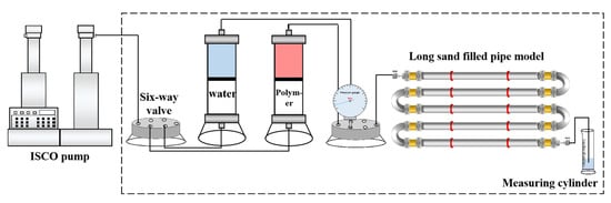
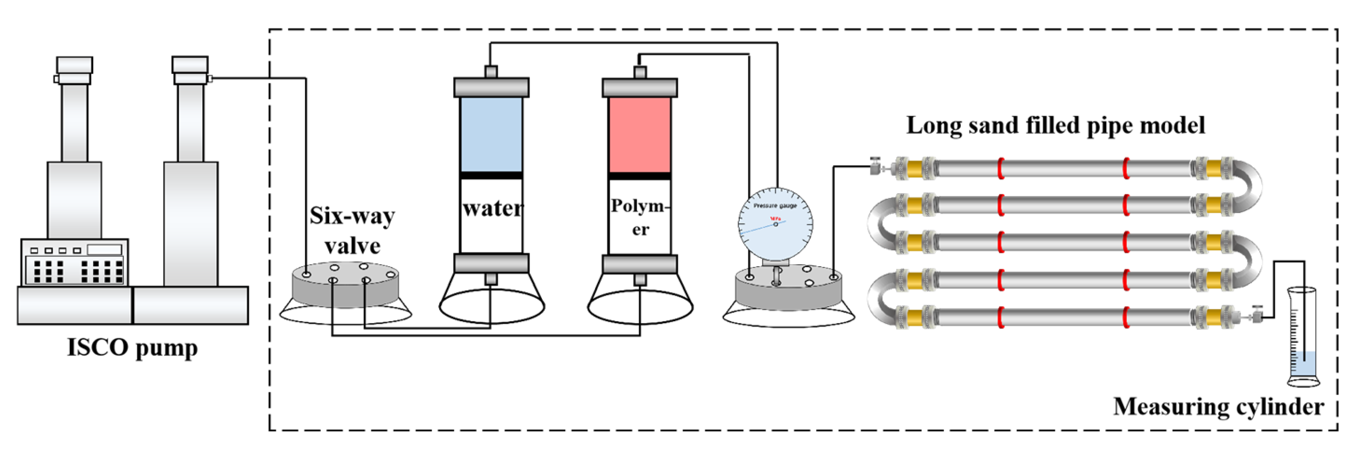
To investigate how well spacing affects polymer viscosity and viscoelasticity during migration, polymer flow experiments were conducted using sand-packed tube models with lengths of 10.6 m and 15 m. These lengths correspond to well spacings of 106 m and 150 m, respectively, based on a 1:10 scaling factor. Sampling points along the tube were used to monitor changes in polymer properties. The physical parameters of the models are listed in

Table 2. Physical parameters of sand-filled pipe model.

Length (cm)	Inside Diameter (cm)	Porosity (%)	Permeability (×10−3 μm2)	Sand Particle Size Range (Mesh)
1060	2.5	25.36	532	70–230
1500	2.5	26.73	515	70–230

, and the experimental setup is shown in Figure 1.

Experimental Procedure: (1) Saturation: The sand-packed tube model was evacuated, saturated with simulated formation water, and then its porosity was measured; (2) Polymer Injection and Sampling: Polymer solution was injected at a constant rate of 0.3 mL/min. After injecting 0.1 PV, the outlet viscosity was measured. Sampling commenced when three consecutive outlet viscosity measurements varied by less than 3%. The outlet valve was then closed, sampling point 1 was opened, and a 40 mL sample was collected. Point 1 was closed, point 2 opened, and this process was repeated sequentially until samples from all points had been collected; (3) Viscosity Measurement: The viscosity of each sample was measured at 45 °C using a Brookfield DV2T viscometer with a UL adapter; (4) Viscoelasticity and Concentration: The viscoelasticity of the samples was measured at 45 °C using a TA Instruments Discovery Hybrid Rheometer (DHR) with a 50 mm-diameter steel parallel-plate geometry (PP50). The polymer concentration was determined using the starch–iodide method. Sampling points were positioned at 10% intervals along the model length to monitor viscosity and viscoelasticity changes. The specific points selected for viscoelasticity and concentration measurements are provided in

Table 3. Distribution of sampling points of sand-filled pipe model.

Proportion of Sampling Distance to Total Length of Model (%)	Distance from Sampling Point to Entrance (m)
	20 m Sand-Filled Pipe Model	30 m Sand-Filled Pipe Model
10	2	3
20	4	6
30	6	9
40	8	12
50	10	15
60	12	18
70	14	21
80	16	24
90	18	27
100	20	30

.

2.3. Plugging Performance Test

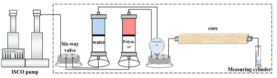
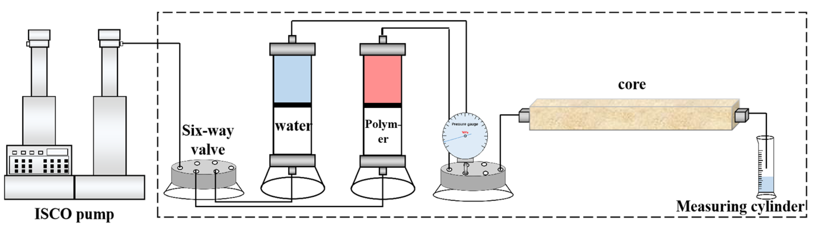
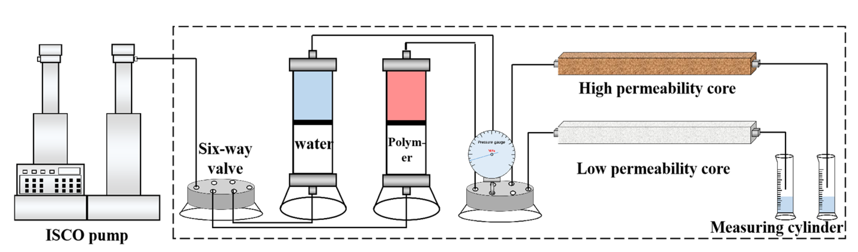
Following the sand-packed tube flow experiments, polymer solutions exhibiting consistent viscosity (as determined in

Table 4. Physical parameters of experimental cores for plugging and resistance enhancement test.

Permeability (×10−3 μm2)	Porosity (%)	Length (cm)	Width (cm)	Height (cm)
275	24.12	30	4.5	4.5

) were extracted from sampling points corresponding to specific migration distances. Core flooding experiments were then conducted to evaluate polymer plugging capacity and resistance enhancement at varying well spacings and migration distances by measuring the resistance coefficient (R_f) and residual resistance coefficient (R_ff). The physical properties of the cores used are listed in Table 4, and the experimental setup is illustrated in Figure 2.

The experimental procedure was as follows: simulated formation water was injected first, followed by the polymer solution and subsequent simulated formation water into the core at a constant rate of 0.3 mL/min until the injection pressure stabilized at each stage. The stabilized pressure differential across the core at each stage was recorded as ΔP₁, ΔP₂, and ΔP₃. The resistance coefficient and residual resistance coefficient were then calculated using Equations (1) and (2).

$${\mathrm{R}}_{\mathrm{f}}={\displaystyle \frac{∆{\mathrm{P}}_1}{∆{\mathrm{P}}_2}}$$

(1)

$${\mathrm{R}}_{\mathrm{f}\mathrm{f}}={\displaystyle \frac{∆{\mathrm{P}}_3}{∆{\mathrm{P}}_1}}$$

(2)

where R_ff—residual resistance coefficient; R_f—resistance coefficient; ΔP₁—differential pressure at both ends after pre water drive; ΔP₂—differential pressure at both ends after polymer flooding; ΔP₃—differential pressure at both ends after subsequent water flooding.

2.4. Profile Improvement Rate Test

The E Reservoir in Daqing Oilfield—the focus of this study—exhibits significant heterogeneity. Permeability distribution variations inevitably impact polymer flooding sweep efficiency, causing preferential flow through high-permeability layers and leaving substantial remaining oil in medium–low permeability zones. Thus, evaluating the profile modification capability of the polymer solution at different well spacings and migration distances is essential.

A dual-core parallel flooding experiment was conducted using cores of contrasting permeabilities (see the experimental setup in Figure 3 and core properties in

Table 5. Physical parameters of experimental cores for profile improvement rate test.

Permeability (×10−3 μm2)	Porosity (%)	Length (cm)	Width (cm)	Height (cm)
275	22.43	30	4.5	4.5
825	27.14	30	4.5	4.5

), employing the polymer solution described in Section 2.4. The experimental procedure was as follows: (1) The cores were evacuated and saturated with simulated formation water; (2) waterflooding was performed at an injection rate of 0.5 mL/min to suppress terminal effects on oil recovery; (3) after pressure stabilization, 1 PV of the chemical profile-control system was injected; (4) post-flush water was injected until pressure and production stabilized. The liquid production rates were recorded after each pressure stabilization phase. The profile improvement rate was calculated using Equation (3).

$$\mathrm{f}={\displaystyle \frac{{\mathrm{r}}_{\mathrm{b}\mathrm{h}}/{\mathrm{r}}_{\mathrm{b}\mathrm{l}}-{\mathrm{r}}_{\mathrm{a}\mathrm{h}}/{\mathrm{r}}_{\mathrm{a}\mathrm{l}}}{{\mathrm{r}}_{\mathrm{b}\mathrm{h}}/{\mathrm{r}}_{\mathrm{b}\mathrm{l}}}}$$

(3)

where f is the profile improvement rate, r_bh is the liquid production rate of the high-permeability layer before injecting the profile control system, r_bl is the liquid production rate of the low-permeability layer before injecting the profile control system, rah is the liquid production rate of the high-permeability layer after injecting the profile control system, and r_al is the liquid production rate of the low-permeability layer after injecting the profile control system.

2.5. Displacement Experiment of Three-Dimensional Heterogeneous Model with Different Sizes

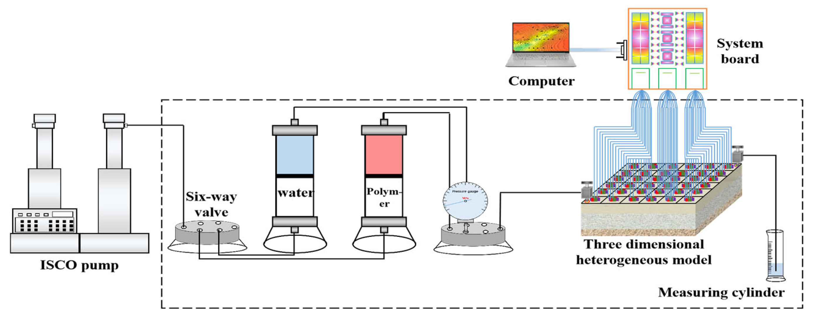
Three-dimensional heterogeneous physical models of varying scales were constructed to investigate how well spacing variations impact polymer flooding efficiency. Displacement experiments integrated with an oil saturation monitoring system revealed the underlying mechanisms. The model schematic and physical parameters are shown in Figure 4 and

Table 6. Physical property parameters of physical model for in layer heterogeneous simulation.

Horizon	Permeability (×10−3 μm2)	Size (cm)	Average Porosity (%)
Low-permeability layer	250	400 × 400 × 45	28.36
Moderately permeable layer	500
Hypertonic layer	750
Low-permeability layer	250	600 × 600 × 45	28.61
Moderately permeable layer	500
Hypertonic layer	750

, respectively. The injection rate was maintained at 0.3 mL/min throughout the displacement experiment.

First, simulated formation water was injected until the recovery rate reached 44%. Then, 1 pore volume (PV) of polymer solution with a viscosity of 45 mPa·s was injected, followed by water flooding until the water cut at the outlet reached 98%. During the experiment, changes in liquid production, water cut, and injection pressure were recorded. Each stage was monitored by the saturation monitoring system. The oil saturation distribution across different permeability layers at each displacement stage was recorded by the oil saturation monitoring system.

3. Results and Discussion

3.1. Variation in Polymer Viscosity with Migration Distance Under Different Well Spacings

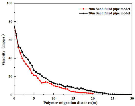
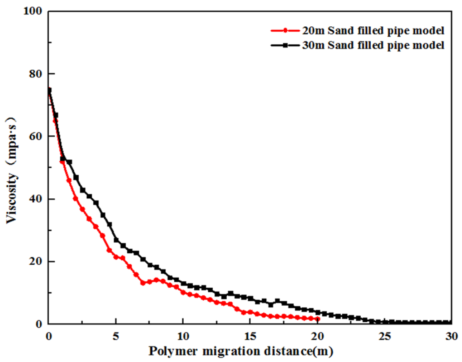
Polymer flow experiments were conducted in sand-packed tube models of varying lengths (20 m and 30 m) to simulate different injector–producer well spacings. Viscosity profiles along the migration path were measured under these conditions. As shown in Figure 5, polymer viscosity decreases with migration distance in both models, exhibiting a rapid decline near the wellbore followed by a gradual reduction. Notably, within the first 3.5 m, viscosity values are comparable between the two models; beyond 3.5 m, the viscosity in the 30 m model exceeds that in the 20 m model at equivalent relative migration distances.

This phenomenon occurs because higher near-wellbore polymer retention in the 30 m model creates a lower average viscosity along the flow path, reducing pressure gradients. Consequently, diminished shear-thinning effects better preserve the polymer’s viscosity at greater distances. Increasing the viscosity of the polymer solution improves the water–oil mobility ratio, M, which is defined as the mobility of the displacement fluid (water) divided by the mobility of the displaced fluid (oil). A more favorable mobility ratio enhances oil recovery. When M < 1, it indicates that the flow capacity of the polymer solution is lower than that of the crude oil, which improves the mobility ratio and can more effectively expand the swept volume. Therefore, for this study, the migration distance at which the polymer solution’s viscosity ensures a favorable mobility ratio (i.e., M < 1) is defined as its effective distance. The effective distances in the 20 m and 30 m sand-packed tube models were 10.5 m and 12.5 m, respectively, which account for 52.5% and 41.7% of their total well spacing. This result indicates that although the absolute effective distance is larger in the 30 m model, its relative effectiveness across the total well spacing is lower than in the 20 m model.

3.2. Variation in Polymer Solution Concentration with Migration Distance

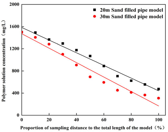
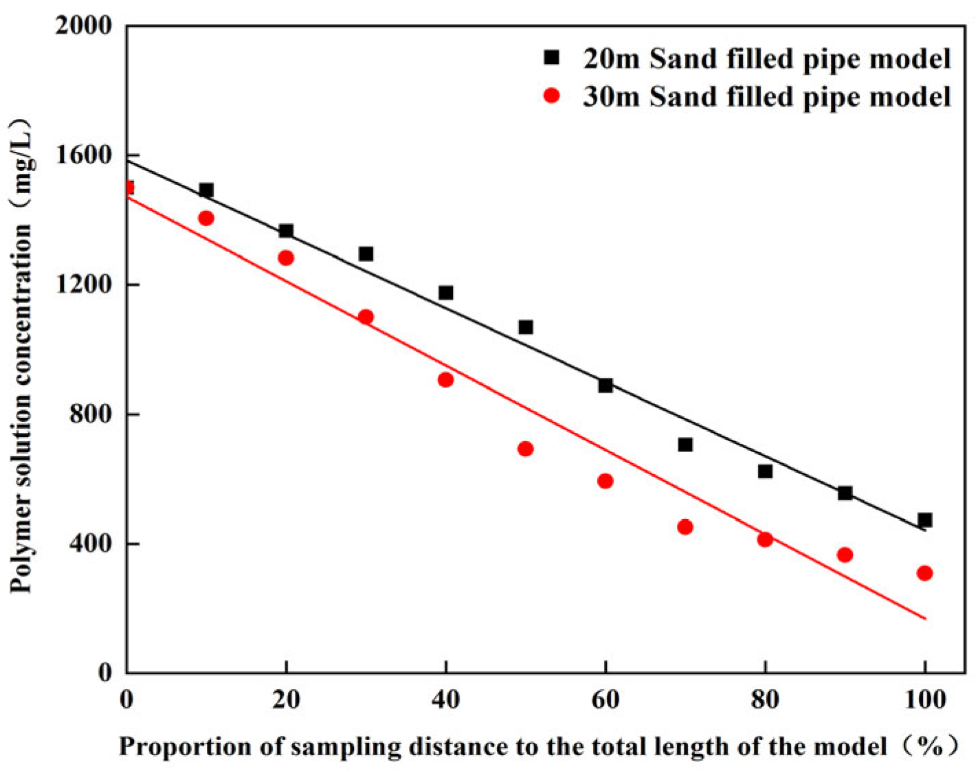
Polymer solution samples were collected at varying migration distances along the sand-packed tube models. Concentration measurements (Figure 6) reveal a monotonic decline with increasing migration distance. This trend primarily results from polymer adsorption onto sand particles and retention within pore throats during flow through the porous medium.

When comparing concentrations at equivalent relative migration distances (sampling point distance/total model length), the 20 m model exhibits higher polymer concentrations than the 30 m model. This occurs because the same relative distance corresponds to a greater absolute migration distance in the longer model. The increased absolute migration distance enhances polymer adsorption and retention, thereby reducing concentration—a finding that is consistent with the viscosity retention mechanism discussed in Section 3.1.

3.3. Variation in Viscoelasticity of Polymer Solution with Migration Distance

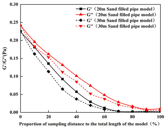
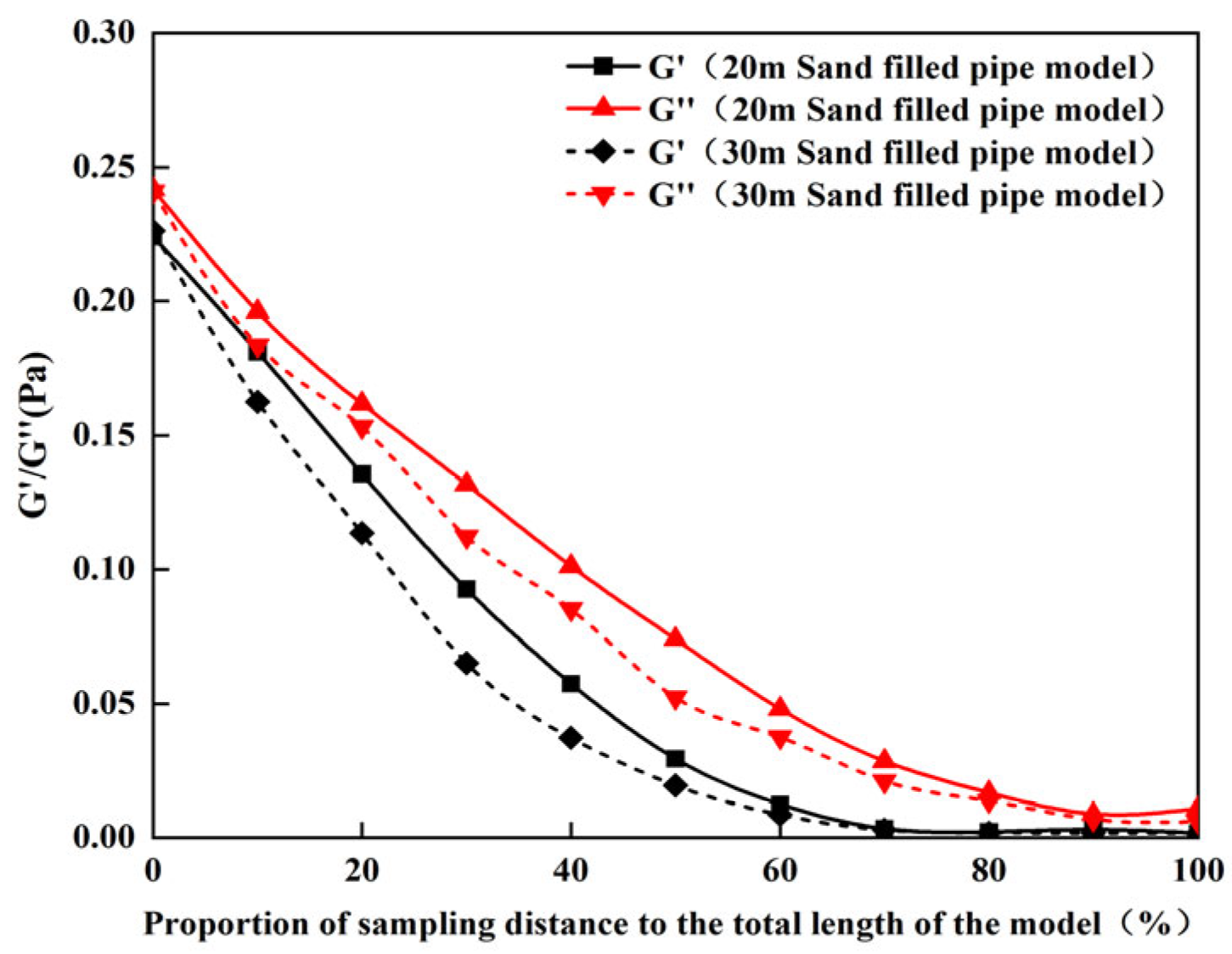
The viscoelastic properties of polymer solutions sampled at varying migration distances along the sand-packed tube models were measured at an angular frequency of 1 s⁻¹ (

Table 7. The variation in viscoelasticity of polymer solutions with the distance of migration.

Proportion of Sampling Distance to Total Length of Model (%)	20 m Sand-Filled Pipe Model		30 m Sand-Filled Pipe Model
	Storage Modulus (G′)	Loss Modulus (G″)	Storage Modulus (G′)	Loss Modulus (G″)
0	0.22414	0.24188	0.2263	0.241
10	0.18107	0.19609	0.1625	0.1836
20	0.13565	0.16176	0.1136	0.1531
30	0.09266	0.13171	0.0652	0.1123
40	0.05746	0.10131	0.0373	0.0852
50	0.02942	0.07406	0.0195	0.0523
60	0.01247	0.04802	0.0086	0.0375
70	0.00338	0.02863	0.003	0.0211
80	0.00224	0.01683	0.0019	0.0138
90	0.00302	0.00889	0.0018	0.0069
100	0.00181	0.01089	0.0017	0.006

and Figure 7). Both the storage modulus (G′) and loss modulus (G″) decrease with increasing migration distance, with G′ exhibiting more rapid attenuation. Beyond 50% of the migration distance, G′ falls below 10% of its initial value and approaches zero at the production end, while G″ consistently exceeds G″ at equivalent distances. These results demonstrate that polymer elasticity diminishes more rapidly than viscosity during migration, with over 90% elasticity loss occurring in the latter half of the model despite retained viscous properties.

Comparative analysis reveals higher G′ and G″ values in the 20 m model than in the 30 m model at equivalent relative migration distances. This occurs because the same fractional distance corresponds to a shorter absolute migration path in the 20 m model. The reduced absolute migration distance decreases shear degradation and adsorption and retention effects, thereby mitigating the decline in viscoelastic moduli.

3.4. Resistance Increasing Performance of Polymer Solution Plugging Varies with Migration Distance

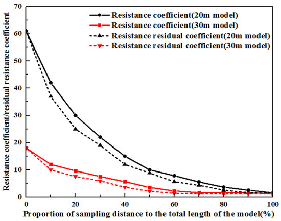
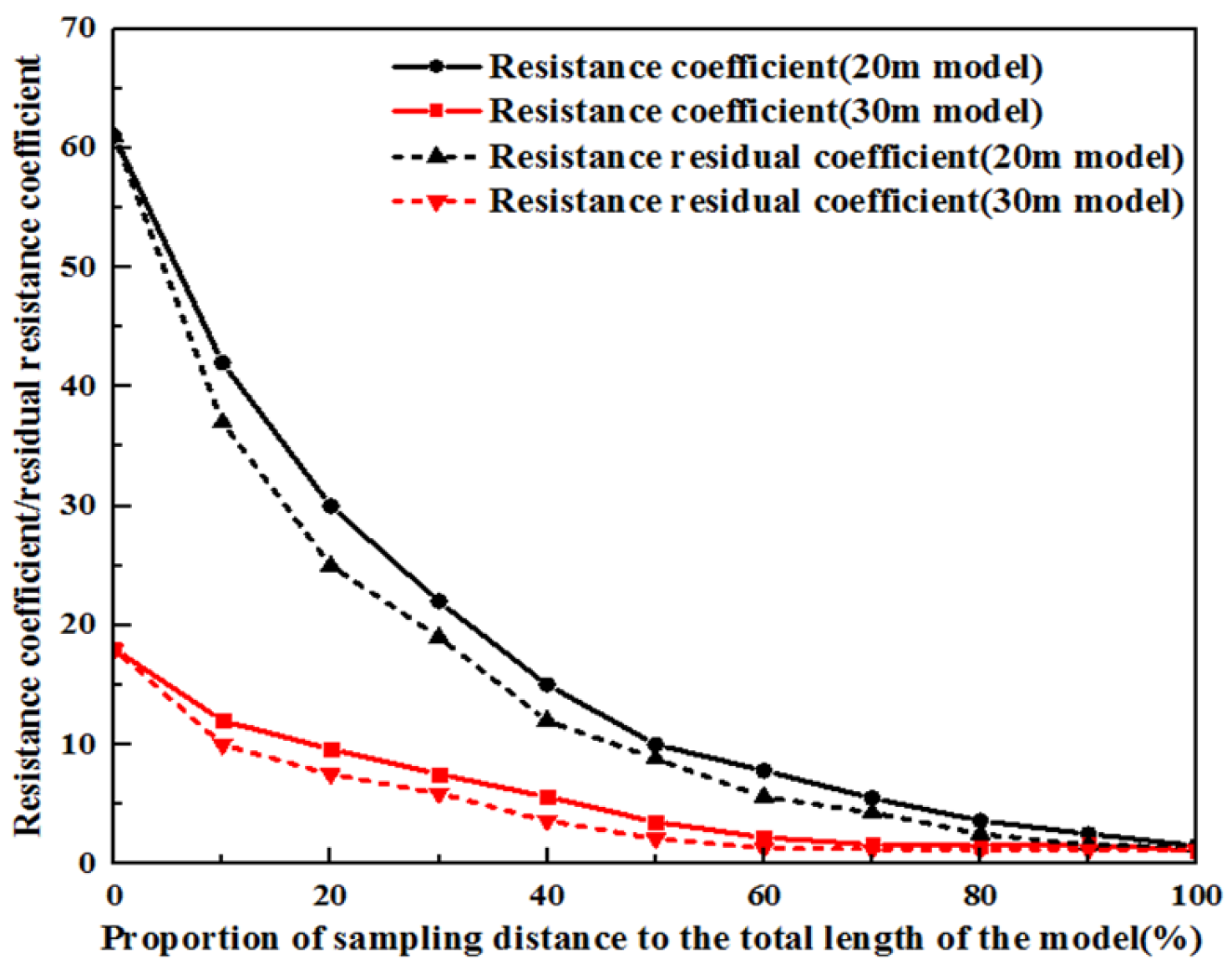
Limited sample volumes from the sand-packed tube model necessitated reconstitution of polymer solutions matching the original viscosity–concentration profiles for subsequent core flooding experiments. These reconstituted solutions were used to measure the resistance coefficient (R_f) and residual resistance coefficient (R_ff) at varying migration distances (Figure 8). Both coefficients decrease with migration distance due to the progressive reduction in polymer concentration, which diminishes molecular adsorption and retention and consequently weakens its plugging capacity and resistance enhancement.

The decline is rapid initially but attenuates beyond 50% migration distance. This biphasic behavior arises from two primary factors: (1) Higher near-wellbore concentrations promote polymer chain entanglement and cross-linking, forming larger hydrodynamic volumes that enhance plugging; (2) As concentration decreases, the probability of chain entanglement is disproportionately reduced, accelerating the initial decline in the coefficients; (3) In the later migration stages, at low concentrations, further reductions minimally affect molecular coil dimensions, thus slowing the coefficient reduction.

At identical relative migration distances, the 20 m model exhibits higher R_f and R_ff values than the 30 m model. This results from the greater absolute migration distance in the 30 m model, causing more severe viscosity and concentration loss and reduced plugging efficiency—a finding consistent with the viscosity (Section 3.1) and concentration (Section 3.2) observations.

3.5. Polymer Solution Profile Improvement Performance Changes with Migration Distance

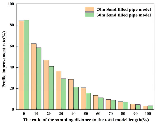
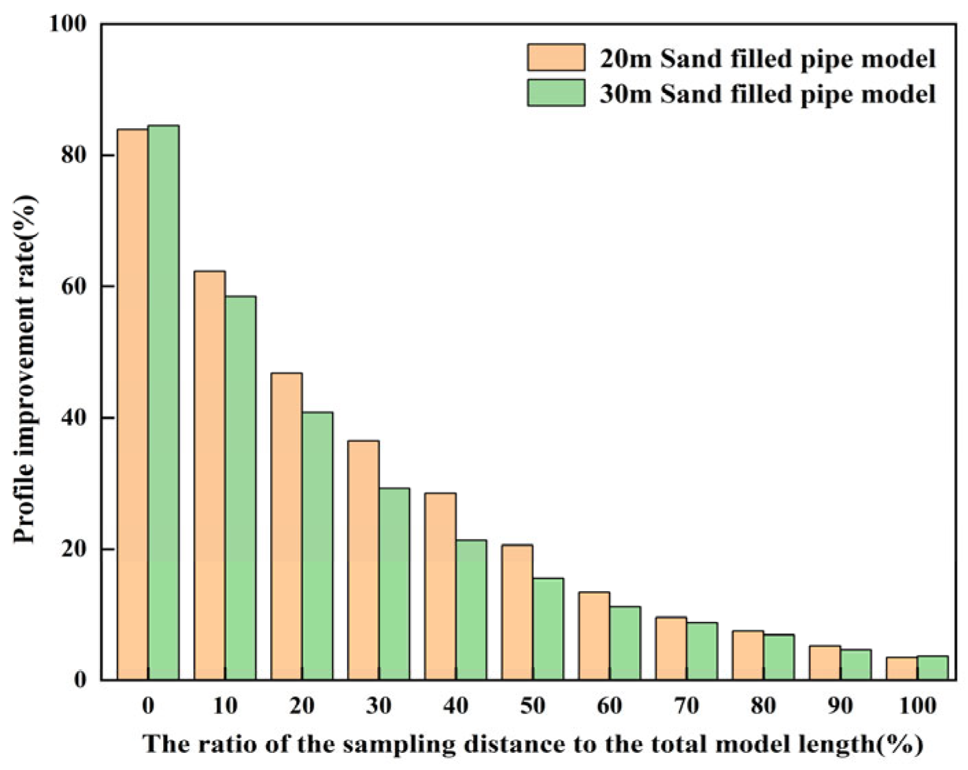
Parallel core flooding experiments using reconstituted polymer solutions were conducted to measure profile improvement rates (η) at varying migration distances (Figure 9). The η values decrease progressively with migration distance, declining from 84% at the inlet—indicating effective conformance control—to 20.6% (20 m model) and 15.5% (30 m model) at 50% distance. By the outlet, η approaches 3% in both models, demonstrating a near-complete loss of profile modification capability. This deterioration results from the reduction in polymer concentration, viscosity, and hydrodynamic volume during migration, which diminishes the differential flow resistance between high- and low-permeability zones.

When comparing equivalent relative migration distances, the 20 m model exhibits significantly higher η values than the 30 m model within the first 60% of the flow path. This divergence stems from a greater viscosity contrast between permeability zones achieved over the shorter absolute migration distance. At later stages (>60% distance), the η values converge as the minimal viscosity differences in both models yield comparable flow resistance distributions.

3.6. Displacement Experiment of Heterogeneous Models Within Three-Dimensional Layers of Different Sizes

Section 3.1, Section 3.2, Section 3.3, Section 3.4 and Section 3.5 demonstrate significant differences in viscosity, concentration, and other polymer properties at equivalent relative migration distances between sand-packed tube models of different lengths. These variations arise from shorter absolute migration distances in the 20 m model. Extrapolating these findings to field conditions indicates that the effective range of the polymer differs across well spacings, ultimately impacting flooding efficiency.

To quantify the effect of well spacing on polymer flooding performance, displacement experiments were conducted in scaled 3D heterogeneous models (40 cm and 60 cm), representing 106 m and 150 m field spacings, respectively. Geometric similarity (with scale ratios of 1:265 and 1:250) guided the model design, as exact replication of field parameters was impractical. This approach preserves critical dimensionless groups while maintaining the viscosity–concentration relationships observed in Section 3.1, Section 3.2 and Section 3.3.

3.6.1. Analysis of Mining Characteristics of Three-Dimensional Heterogeneous Model with Different Sizes

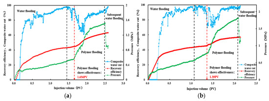
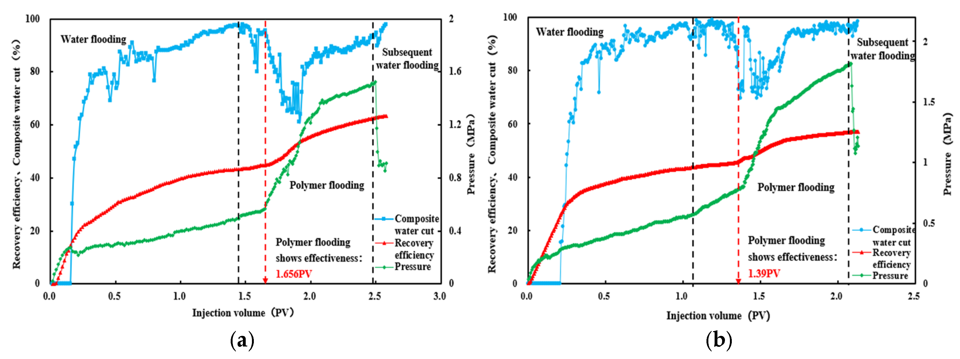
The production curves for the heterogeneous models of different scales are shown in Figure 10. For the 40 cm model (Figure 10a): Waterflooding achieved a 43.38% recovery, with rapid production during the water-free period, followed by slowed recovery and a rapid water cut increase after breakthrough. Polymer flooding (1 PV slug) added 19.10% recovery, yielding a total recovery of 62.47%. The polymer response initiated at 0.194 PV injected, with a maximum water cut reduction of 36.89%; the average water cut during polymer flooding was 66.68%, confirming effective conformance control. For the 60 cm model (Figure 10b): Waterflooding yielded a 43.79% recovery, exhibiting similar breakthrough behavior. The polymer response initiated later (at 0.31 PV injected), with a 28.61% maximum water cut reduction. Polymer flooding added 13.3% recovery at an average water cut of 73.37%. Comparative analysis reveals earlier polymer effectiveness in the smaller well spacing (0.194 PV vs. 0.31 PV), a greater water cut reduction in the 40 cm model (36.89% vs. 28.61%), and an enhanced recovery contribution from polymer flooding in the smaller spacing (19.10% vs. 13.3%).

These results demonstrate that reduced well spacing accelerates polymer effectiveness, enhances water cut reduction, and improves ultimate recovery in heterogeneous reservoirs. The delayed response in the larger well spacing correlates with the extended migration requirements observed in Section 3.1, Section 3.2, Section 3.3, Section 3.4 and Section 3.5.

3.6.2. Mechanism Analysis of Influence of Well Spacing Change on Polymer Flooding Development Effect

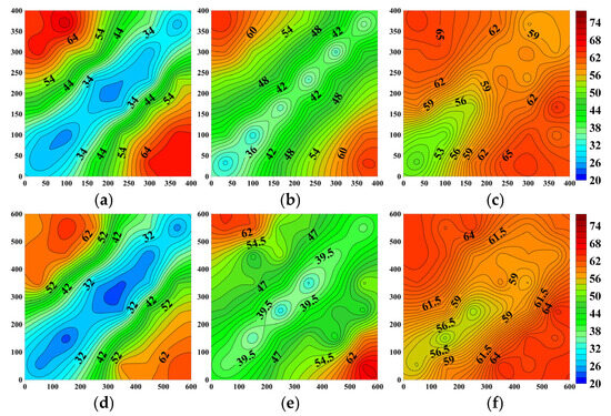
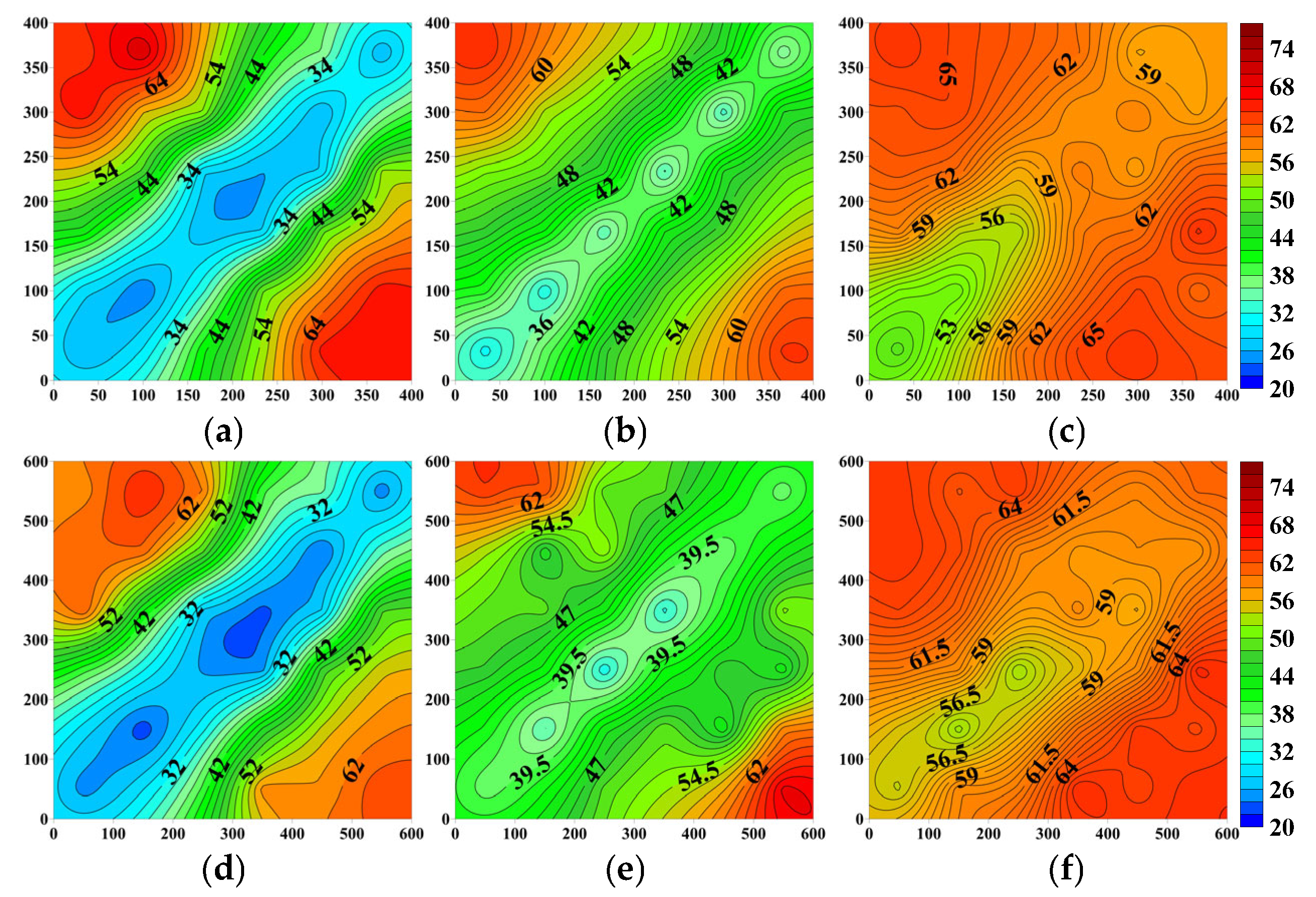
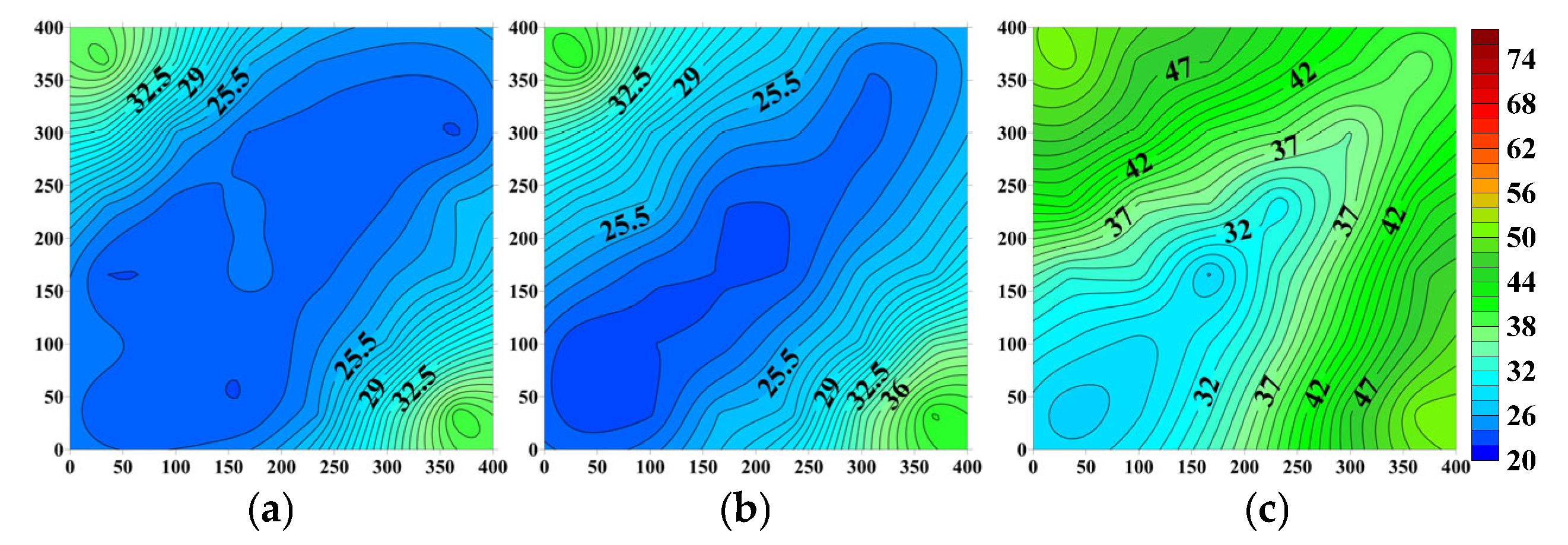
To further investigate the mechanism by which well spacing influences polymer flooding performance, oil saturation distribution across different displacement stages and permeability layers was measured using an oil saturation monitoring system. The resulting saturation distribution is visualized in the cloud map in Figure 11.

In the crude oil saturation cloud map, The x and y axes represent the physical dimensions of the three-dimensional model in millimeters (mm). The color gradient represents the variation in oil saturation values, with the color bars indicating the saturation scale from 0 to 400 mm (Figure 11a–c) and 0 to 600 mm (Figure 11d–f). The numerical values displayed within the contours (e.g., 25.5, 47, 42, 54.5, etc.) indicate precise oil saturation measurements at specific monitoring locations.

The oil saturation distribution for the 40 cm and 60 cm models after water flooding is presented in Figure 11. The figure indicates similar development characteristics across the layers in both models: crude oil in the high-permeability layers is preferentially swept during water flooding, while development in the medium- and low-permeability layers remains limited. Post-flooding, the high-permeability layers in both models exhibit well-defined seepage channels along the main flow paths, with over 70% of their area swept. Although oil saturation decreases significantly along the main flow paths in the medium-permeability layers, neither model develops continuous seepage channels within them. The medium-permeability layers achieve approximately 40% sweep efficiency, whereas the low-permeability layers show minimal development, with oil saturation reduction confined to the immediate vicinity of the injection well.

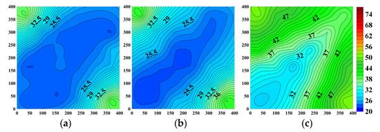
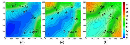
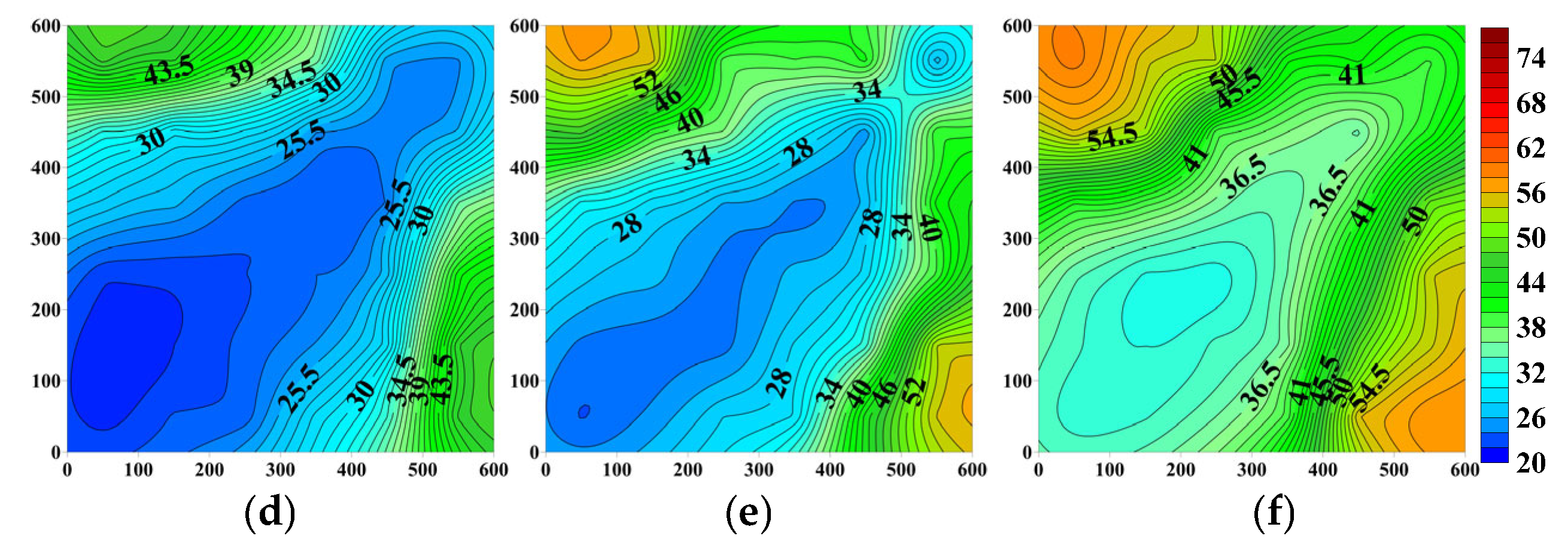
The oil saturation distribution for the 40 cm and 60 cm models after polymer flooding is presented in Figure 12. The results demonstrate that the high- and medium-permeability layers in the 40 cm model were effectively swept, with the sweep efficiency of the low-permeability layer exceeding 50%. In contrast, the 60 cm model was primarily drained through the high-permeability layer, with only moderate development of the medium-permeability layer, the sweep efficiency of which remained significantly lower than in the 40 cm model. The low-permeability layer in the 60 cm model exhibited poor production performance. This is attributed to reservoir heterogeneity, which causes the polymer to preferentially migrate through the high- and medium-permeability layers that offer lower flow resistance, consequently limiting the development of the low-permeability layer.

The diagrams visualize the oil saturation field captured by the in situ monitoring system after water flooding (Figure 11) and polymer flooding (Figure 12) for both the 40 cm and 60 cm three-dimensional heterogeneous models. Each figure comprises six panels (a–f), showing the high-, medium-, and low-permeability layers for each model size. The color gradient, from red (high oil saturation) to blue (low oil saturation), illustrates the efficiency of oil displacement. For instance, in Figure 11 after water flooding, the high-permeability layers (panels a and d) show extensive blue channels along the main flow paths, indicating successful water sweep, while the medium-permeability layers (panels b and e) display a mottled pattern of red and blue, signifying partial and uneven development. The low-permeability layers (panels c and f), in contrast, remain largely red with only minor blue patches near the injection point, confirming very limited oil mobilization. A critical comparison in Figure 12 after polymer flooding reveals that in the 40 cm model, the swept (blue) area expands significantly into the medium- and even low-permeability layers (panels b and c), demonstrating more uniform displacement. Conversely, in the 60 cm model (panels e and f), the expansion of the swept region in these layers is markedly less pronounced, with the low-permeability layer remaining largely unaffected.

A comparative analysis of the oil saturation distribution patterns across injection stages and permeability layers reveals that the 40 cm model achieves higher sweep efficiency within equivalent permeability layers at identical polymer injection volumes. Integrating these observations with prior experimental results indicates that reduced well spacing increases the proportion of the effective polymer propagation distance. This enables more extensive crude oil displacement within a given permeability layer, thereby enhancing the polymer sweep efficiency. Additionally, crude oil production from medium- and low-permeability layers is substantially greater in the 40 cm model. This is primarily because the diminished influence of reservoir heterogeneity at reduced well spacing allows the polymer’s plugging capacity, resistance enhancement, and profile modification to function more effectively across a greater reservoir volume, ultimately resulting in superior development performance in the 40 cm model compared to the 60 cm model.

4. Conclusions

In this paper, experiments were conducted to investigate the changes in polymer properties and EOR performance under different well spacing conditions:

(1) The effective propagation distances of the polymer solution in the models simulating different well spacings are 10.5 m and 12.5 m, corresponding to 55% and 41.7% of the respective injector–producer distances. Although the absolute propagation distance is greater in the larger well spacing model, the proportion of the well spacing effectively utilized by the polymer is smaller than in the model with smaller well spacing.

(2) In the smaller well spacing model, the polymer solution experiences relatively lower shear and adsorption within the porous media. Consequently, at equivalent relative migration distances (distance traveled/total well spacing), the viscosity, storage modulus, and loss modulus of the polymer solution decrease more rapidly in the larger well spacing model.

(3) At the same relative migration distance, the polymer solution in the smaller well spacing model achieves higher plugging efficiency and greater conformance improvement. It also plugs the low-permeability layers more effectively and demonstrates superior deep conformance control.

(4) The oil recovery factor for the model simulating a 106 m well spacing is 5.79% higher than that for the model simulating a 150 m well spacing. Polymer breakthrough occurs earlier in the 106 m model (at 0.194 PV) than in the 150 m model (at 0.302 PV). After injecting 1.0 PV of polymer, the 106 m model exhibits higher polymer viscosity retention and a larger effectively swept area than the 150 m model. This enables more efficient oil mobilization from the main flow paths near the production well. Post-polymer flooding, the primary locations of remaining oil differ: in the 106 m model, it is predominantly located in non-main flow areas of high- and medium-permeability layers and in areas outside the main flow paths in low-permeability layers. In contrast, the 150 m model shows remaining oil concentrated in non-main flow areas of high- and medium-permeability layers, within the main flow paths near the production well, and in areas outside the main flow paths in the low-permeability layers.

References

- Wu, Y.; Li, P.; Yan, B.; Li, X.; Huang, Y.; Yuan, J.; Feng, X.; Dai, C. A salt-induced tackifying polymer for enhancing oil recovery in high salinity reservoirs: Synthesis, evaluation, and mechanism. Green Energy Environ. 2024, 9, 1747–1758. [Google Scholar] [CrossRef] [Scilit]
- Yuan, S.; Han, H.; Wang, H.; Luo, J.; Wang, Q.; Lei, Z.; Xi, C.; Li, J. Research progress and potential of new enhanced oil recovery methods in oilfield development. Pet. Explor. Dev. 2024, 51, 963–980. [Google Scholar] [CrossRef] [Scilit]
- Kang, W.-L.; Zhou, B.-B.; Issakhov, M.; Gabdullin, M. Advances in enhanced oil recovery technologies for low permeability reservoirs. Pet. Sci. 2022, 19, 1622–1640. [Google Scholar] [CrossRef] [Scilit]
- Prakash, S.; Joshi, D.; Ojha, K.; Mandal, A. Enhanced oil recovery using polymer alternating CO2 gas injection: Mechanisms, efficiency, and environmental benefits. Energy Fuels 2024, 38, 5676–5689. [Google Scholar] [CrossRef] [Scilit]
- Song, H.; Ghosh, P.; Bowers, A.; Niu, F.; Mohanty, K. Low-Salinity Polymer Flood for Enhanced Oil Recovery in Low-Permeability Carbonates. SPE J. 2024, 29, 443–454. [Google Scholar] [CrossRef] [Scilit]
- Hu, J.; Jiang, P.; Zhang, G.; Ge, J.; Pei, H. Study on Polymer Flooding Profile Control and Antimony Technology. In Proceedings of the 2nd International Conference on Material Science, Energy and Environmental Engineering (MSEEE 2018), Xi’an, China, 16–17 August 2018; p. 5. [Google Scholar] [CrossRef] [Scilit]
- Zheng, X.; Shi, J.; Cao, G.; Yang, N.; Cui, M.; Jia, D.; Liu, H. Progress and prospects of oil and gas production engineering technology in China. Pet. Explor. Dev. 2022, 49, 644–659. [Google Scholar] [CrossRef] [Scilit]
- Mohammadi, M.H.; Kulakhmetovna, Y.A.; Joia, R. An overview of oil recovery techniques: From primary to enhanced oil recovery methods. J. Res. Appl. Sci. Biotechnol. 2024, 3, 291–301. [Google Scholar] [CrossRef] [Scilit]
- Yu, H.; Wang, Y.; Zhang, L.; Zhang, Q.; Guo, Z.; Wang, B.; Sun, T. Remaining oil distribution characteristics in an oil reservoir with ultra-high water-cut. Energy Geosci. 2024, 5, 100116. [Google Scholar] [CrossRef] [Scilit]
- Zhang, S.; Zhang, T.; Zhang, X.; Yan, M. Formation mechanism and distribution characteristics of micro residual oil in ultra-high water cut reservoirs a case study of yangsanmu oilfield. In Proceedings of the Fourth International Conference on Energy Engineering and Environmental Protection, Xiamen, China, 19–21 November 2019; Volume 467, p. 012017. [Google Scholar] [CrossRef] [Scilit]
- Xu, Z.-X.; Li, S.-Y.; Li, B.-F.; Chen, D.-Q.; Liu, Z.-Y.; Li, Z.-M. A review of development methods and EOR technologies for carbonate reservoirs. Pet. Sci. 2020, 17, 990–1013. [Google Scholar] [CrossRef] [Scilit]
- Pashchenko, A.O.; Borodina, A.N.; Yavorska, O.; Ishkov, V.V.; Cherniaiev, O.V. Application of polymer flooding to increase oil recovery. In Proceedings of the 5th International Conference on Sustainable Futures: Environmental, Technological, Social and Economic Matters, Kryvyi Rih, Ukraine, 21–24 May 2024; Volume 1415, p. 012054. [Google Scholar] [CrossRef] [Scilit]
- Leon, J.M.; Masalmeh, S.K. Evaluation of Alternative Polymer-Based EOR Mechanisms to Improve Sweep Efficiency and Water Management in Complex Light Oil Carbonate Reservoirs in Abu Dhabi. In Proceedings of the SPE Conference at Oman Petroleum & Energy Show, Muscat, Oman, 12–14 May 2025. [Google Scholar] [CrossRef] [Scilit]
- Gbadamosi, A.; Patil, S.; Kamal, M.S.; Adewunmi, A.A.; Yusuff, A.S.; Agi, A.; Oseh, J. Application of Polymers for Chemical Enhanced Oil Recovery: A Review. Polymers 2022, 14, 1433. [Google Scholar] [CrossRef] [Scilit]
- Karimov, D.; Toktarbay, Z. Enhanced oil recovery: Techniques, strategies, and advances. ES Mater. Manuf. 2023, 23, 1005. [Google Scholar] [CrossRef] [Scilit]
- Yu, Q.; Liu, Y.; Liang, S.; Tan, S.; Sun, Z.; Yu, Y. Experimental study on surface-active polymer flooding for enhanced oil recovery: A case study of Daqing placanticline oilfield, NE China. Pet. Explor. Dev. 2019, 46, 1206–1217. [Google Scholar] [CrossRef] [Scilit]
- Tan, F.-Q.; Ma, C.-M.; Qin, J.-H.; Li, X.-K.; Liu, W.-T. Factors influencing oil recovery by surfactant-polymer flooding in conglomerate reservoirs and its quantitative calculation method. Pet. Sci. 2022, 19, 1198–1210. [Google Scholar] [CrossRef] [Scilit]
- Zhang, X.; Yu, J.; Liu, L.; Liu, X.; Lu, X.; Feng, Q. Experimental Investigation of Synergistic Enhanced Oil Recovery by Infill Well Pattern and Chemical Flooding After Polymer Flooding. Gels 2025, 11, 660. [Google Scholar] [CrossRef] [Scilit] [PubMed]
- Olabode, O.; Dike, H.; Olaniyan, D.; Oni, B.; Faleye, M. Experimental investigation of the effect of surfactant–polymer flooding on enhanced oil recovery for medium crude oil. Polymers 2024, 16, 1674. [Google Scholar] [CrossRef] [Scilit]
- Sun, X.; Zhao, M.; Fan, X.; Zhang, Y.; Xu, C.; Wang, L.; Sang, G. Study on micro production mechanism of corner residual oil after polymer flooding. Polymers 2022, 14, 878. [Google Scholar] [CrossRef] [Scilit]
- Ameli, F.; Moghadam, S.; Shahmarvand, S. Polymer flooding. In Chemical Methods; Gulf Professional Publishing: Cambridge, MA, USA, 2022; pp. 33–94. [Google Scholar] [CrossRef] [Scilit]
- Yan, Y.; Wang, L.; Sang, G.; Han, X. Influence of polymer viscoelasticity on microscopic remaining oil production. Polymers 2022, 14, 940. [Google Scholar] [CrossRef] [Scilit]
- Dafaalla, M.; Azad, M.S.; Ayirala, S.; Alotaibi, M.; Fahmi, M.; Saleh, S.; Al Shehri, D.; Mahmoud, M. Potential of polymer’s viscosity and viscoelasticity for accessible oil recovery during low salinity polymer flooding in heterogeneous carbonates. Fuel 2025, 379, 133008. [Google Scholar] [CrossRef] [Scilit]
- He, J.; Jin, X.; Liu, X.; Yuan, L.; Liu, R.; Chen, S.; Wu, H.; Yang, W.; Wang, J.; Zhang, H.; et al. Comprehensive Study on Viscosity-Increasing and Oil Displacement Characteristics of Functional Polymer. Processes 2025, 13, 1859. [Google Scholar] [CrossRef] [Scilit]
- Seright, R.S.; Wang, D. Polymer flooding: Current status and future directions. Pet. Sci. 2023, 20, 910–921. [Google Scholar] [CrossRef] [Scilit]
- Kummar, S.; Dull, N.R.; Helsper, S.; Liberatore, M.W. Effect of shear rate, temperature, and salts on the viscosity and viscoelasticity of semi-dilute and entangled xanthan gum. J. Appl. Polym. Sci. 2025, 142, e56372. [Google Scholar] [CrossRef] [Scilit]
- Howe, A.M.; Clarke, A.; Giernalczyk, D. Flow of concentrated viscoelastic polymer solutions in porous media: Effect of MW and concen-tration on elastic turbulence onset in various geometries. Soft Matter 2015, 11, 6419–6431. [Google Scholar] [CrossRef] [Scilit] [PubMed]
- Clarke, A.; Howe, A.M.; Mitchell, J.; Staniland, J.; Hawkes, L.; Leeper, K. Mechanism of anomalously increased oil displacement with aqueous viscoelastic polymer solutions. Soft Matter 2015, 11, 3536–3541. [Google Scholar] [CrossRef] [Scilit] [PubMed]
- Wang, D.; Dong, H.; Lv, C.; Fu, X.; Nie, J. Review of Practical Experience by Polymer Flooding at Daqing. SPE Reserv. Eval. Eng. 2009, 12, 470–476. [Google Scholar] [CrossRef] [Scilit]
- Sun, T.; Liu, H.; Zhang, Y. The impact of well spacing on three-dimensional in situ extraction of oil shale using high-temperature air injection. Phys. Fluids 2024, 36, 036606. [Google Scholar] [CrossRef] [Scilit]
- Mukhametshin, V.V.; Gilyazetdinov, R.A.; Kuleshova, L.S.; Novruzova, S.H.; Askerov, V.M. On the depth of identification of objects in the study of the influence of the density of the grid of wells on the degree of production of oil reserves. Horizons 2024, 26, 28. [Google Scholar] [CrossRef] [Scilit]
- Al-Khdheeawi, E.A.; Al-Rubuey, W.I.; Yuan, Y.; Fahem, M.M.; Jassim, J.J. Well Spacing Optimization to Enhance the Performance of Tight Reservoirs. Pet. Chem. 2024, 64, 829–839. [Google Scholar] [CrossRef] [Scilit]
- Mukhametshin, V.S.; Kuleshova, L.; Yakupov, R.; Vafin, R.; Gilyazetdinov, R. Features of localization of remaining oil in terrigenous reservoirs and potential for their recovery at the final stage of field development. In Proceedings of the II International Scientific and Practical Conference “Energy, Ecology and Technology in Agriculture” (EEA2023), Khujand, Tajikistan, 11 December 2023; Volume 480, p. 01018. [Google Scholar] [CrossRef] [Scilit]
- Fu, D.; Fu, Y.; Zhang, Y.; Wang, M. Experimental simulation study on influencing factors of liquid production capacity in heterogeneous water drive reservoirs. Phys. Fluids 2024, 36, 016612. [Google Scholar] [CrossRef] [Scilit]
- Du, J.; Lv, C.; Lan, X.; Song, J.; Liu, P.; Chen, X.; Wang, Q.; Liu, J.; Guo, G. A review on viscosity retention of PAM solution for polymer flooding technology. Pet. Sci. Technol. 2024, 42, 372–405. [Google Scholar] [CrossRef] [Scilit]
Disclaimer/Publisher’s Note: The statements, opinions and data contained in all publications are solely those of the individual author(s) and contributor(s) and not of MDPI and/or the editor(s). MDPI and/or the editor(s) disclaim responsibility for any injury to people or property resulting from any ideas, methods, instructions or products referred to in the content. |
© 2025 by the authors. Licensee MDPI, Basel, Switzerland. This article is an open access article distributed under the terms and conditions of the Creative Commons Attribution (CC BY) license (https://creativecommons.org/licenses/by/4.0/).