
Adaptive Scale and Correlative Attention PointPillars: An Efficient Real-Time 3D Point Cloud Object Detection Algorithm

Abstract
1. Introduction
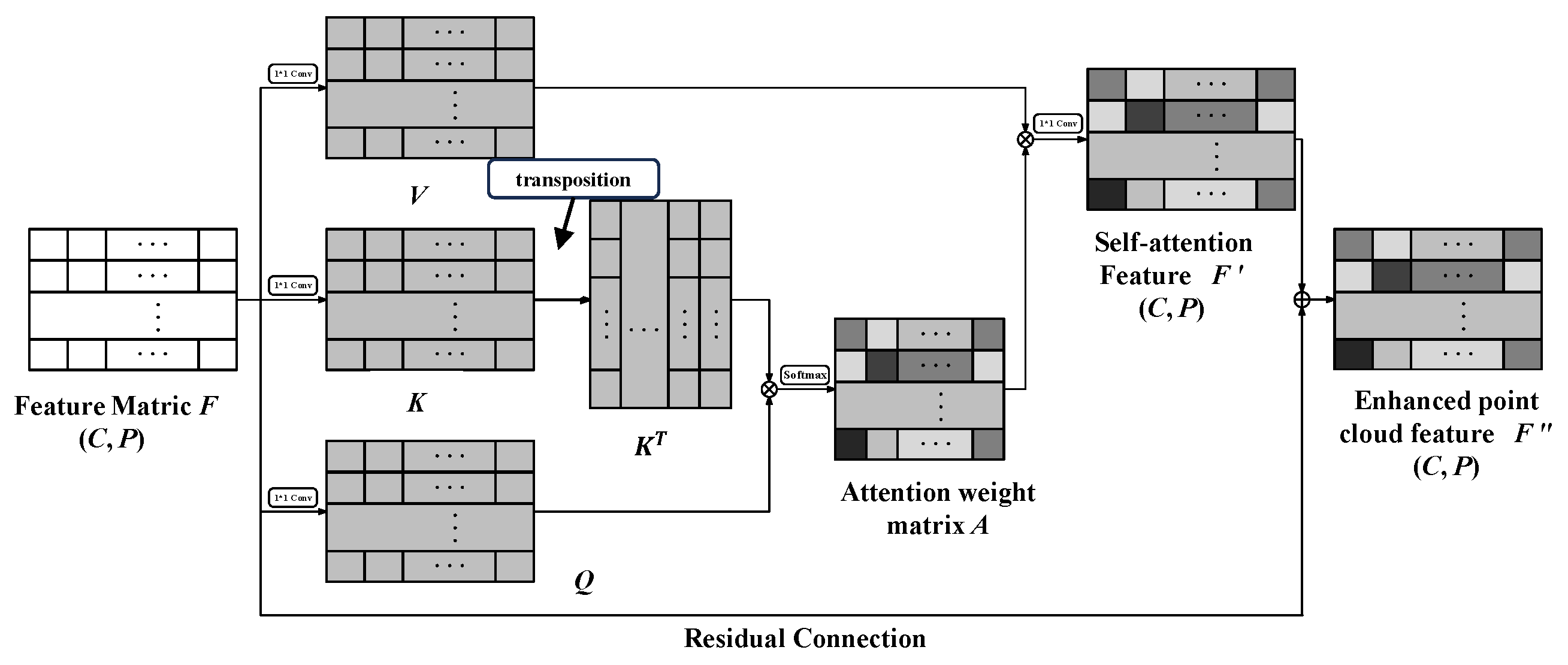
- This study proposes an object recognition algorithm called ASCA-PointPillars. In the algorithm, we design an ASP module that innovatively utilizes multi-scale pillars to encode point clouds, effectively reducing the loss of spatial information. Subsequently, a CPA module is employed to establish contextual associations within a pillar’s point cloud, thereby enhancing the point cloud’s features.
- A data augmentation algorithm called RS-Aug is proposed, leveraging semantic information to identify reasonable areas for placing ground truths, addressing the issue of imbalanced categories in datasets.
2. Related Works
3. Method
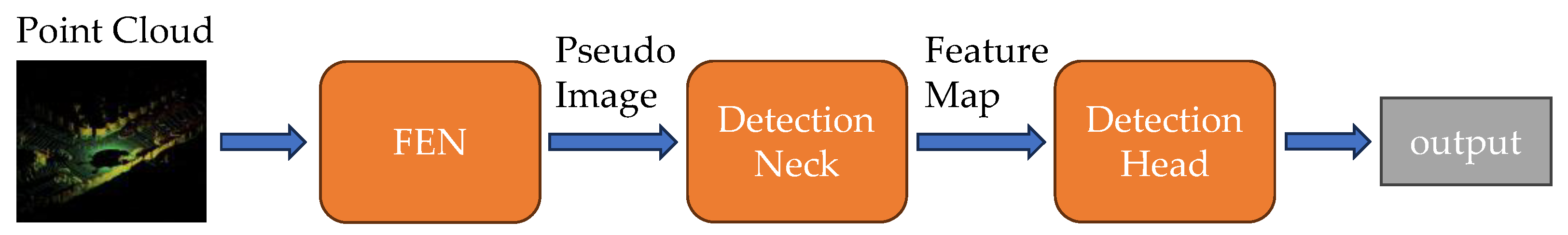
3.1. Overall Architecture of ASCA-PointPillars
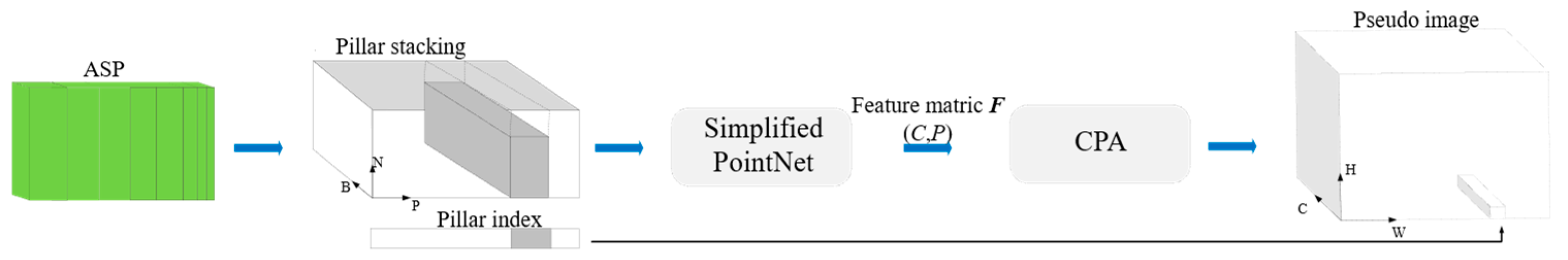
3.2. Feature Encoding Network
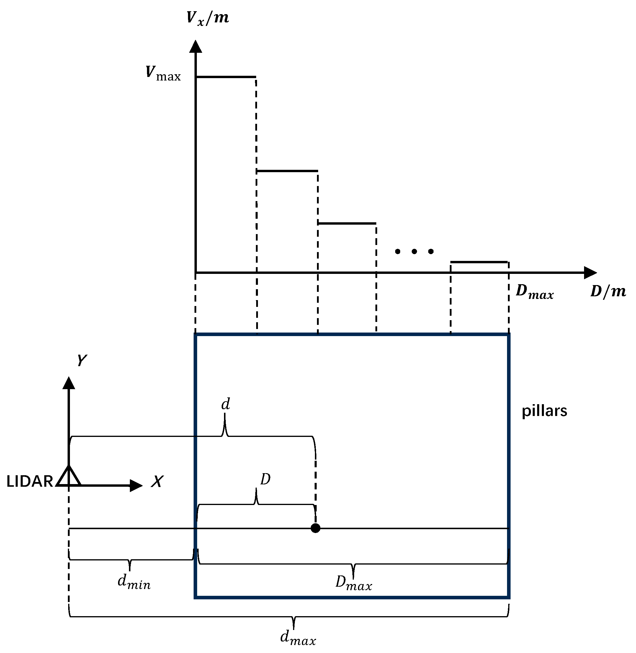
- ASP module
- 2.
- CPA module
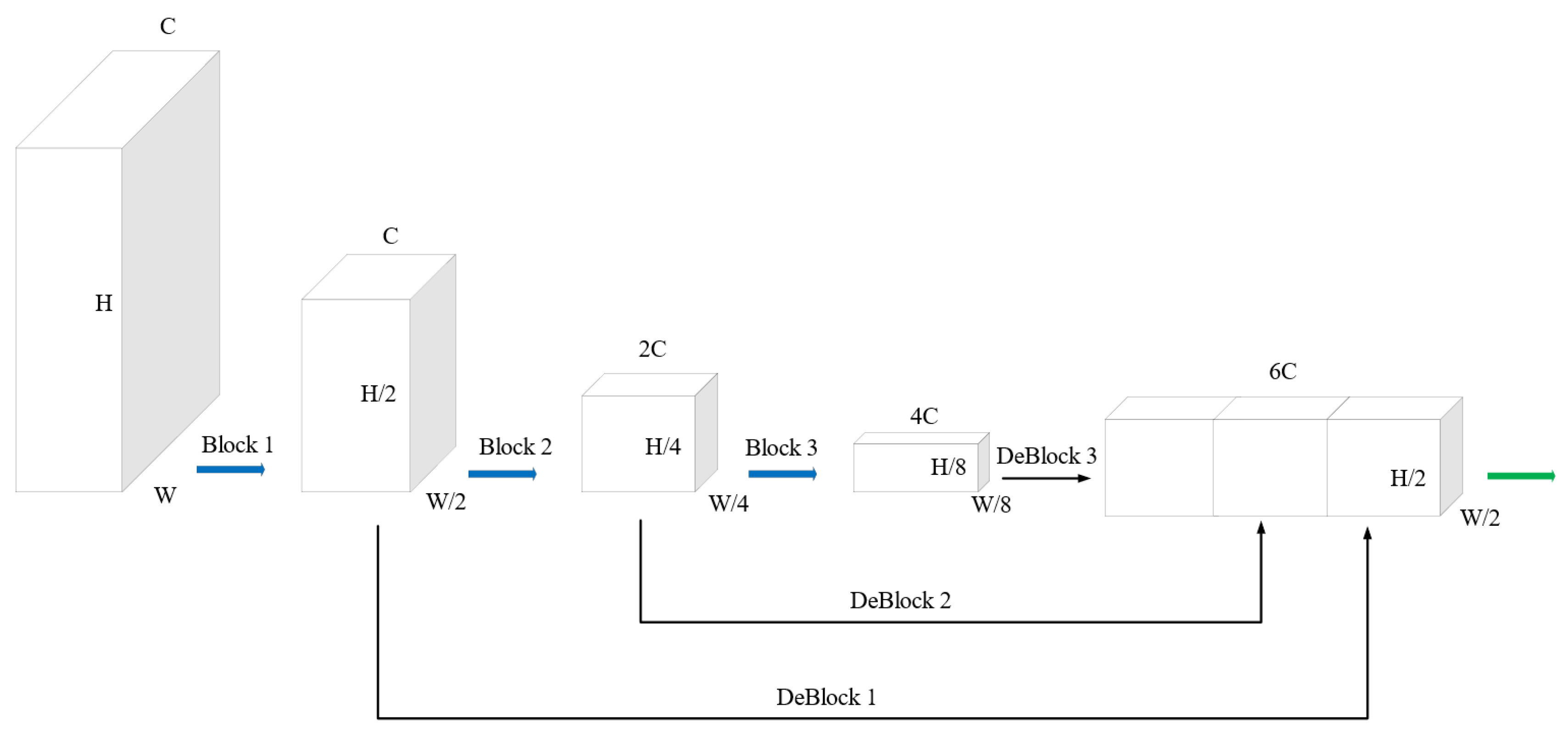
3.3. Detection Neck
3.4. Loss Function
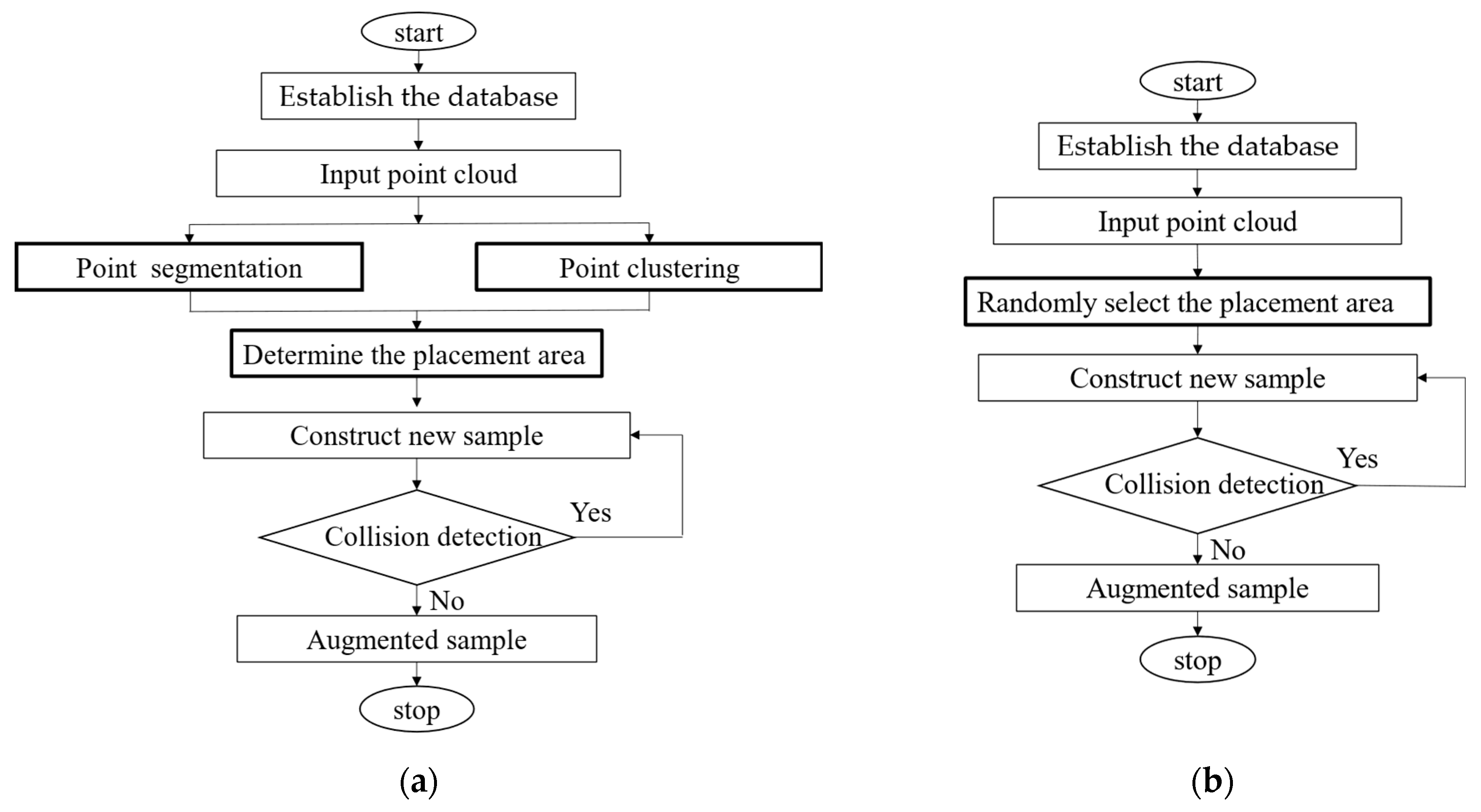
3.5. RS-Aug Algorithm
- Establish the database. Establish a database that includes all the ground truths (bounding boxes and the points inside them). For instance, in our following experiment, three categories of ground truths are included. They are vehicles, cyclists, and pedestrians.
- Segment the ground and non-ground points. Input a training sample, then apply the RANSAC algorithm to segment the non-ground points and ground points and obtain ground fitting parameters.
- Points clustering. Utilize the DBSCAN algorithm to cluster non-ground points, thereby obtaining clusters of non-ground points.
- Determine the placement area. Obtain the semantic information of the current scene through Steps 2 and 3, classifying the point cloud into ground and non-ground points. Subsequently, apply the Minimum Bounding Rectangle algorithm to fit the bounding boxes of the non-ground point clusters, acquiring the position and size of the bounding boxes. Using the size and position information, exclude the regions occupied by the bounding boxes from the ground area identified in Step 2, leaving the remaining space as the designated area for placement.
- Construct a new sample. Randomly select the ground truths from the database based on the proportions of different categories appearing in the training dataset. Then, randomly insert ground truths into the designated placement area.
- Collision checking. Check whether the newly placed point cluster collides with the existing point clusters. If a collision is detected, repeat step (5) and then perform the collision check again. If no collision is detected, the enhanced data will be fed into the network for training, and this process ends.
4. Experiment and Result Analysis
4.1. Experimental Setup
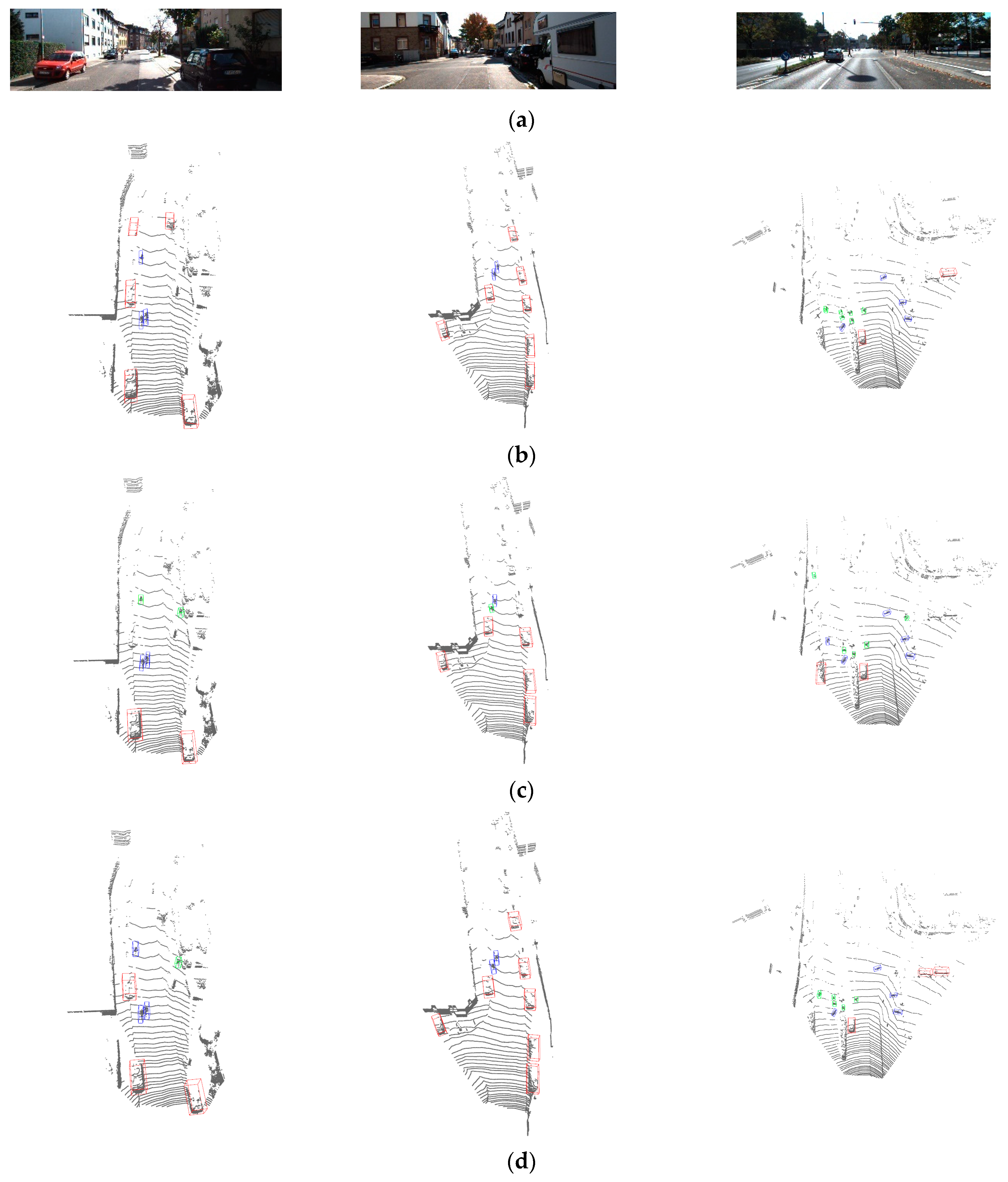
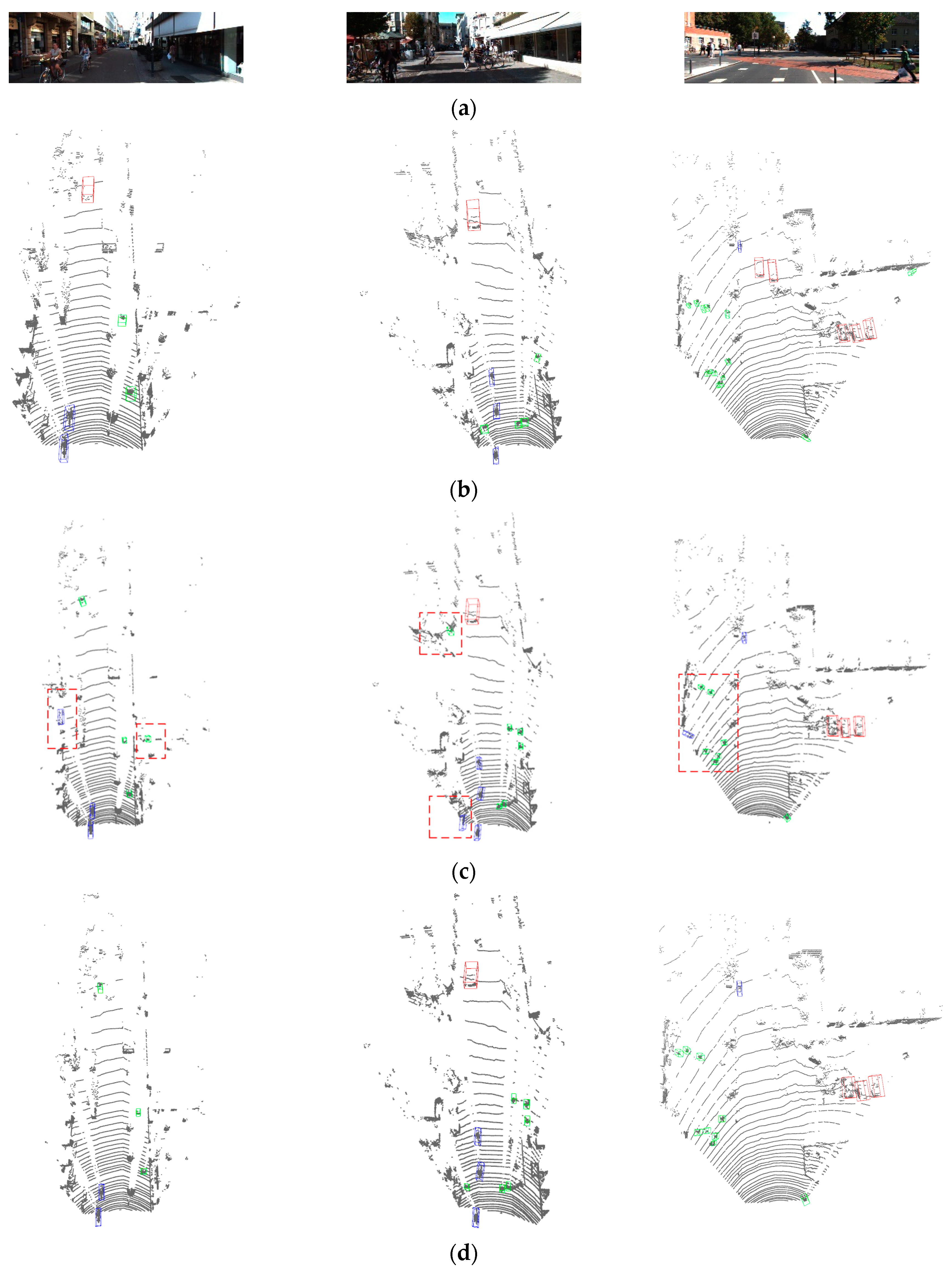
4.2. Experimental Results
4.3. Ablation Experiment
5. Conclusions
Author Contributions
Funding
Institutional Review Board Statement
Informed Consent Statement
Data Availability Statement
Conflicts of Interest
References
- Qi, C.R.; Su, H.; Mo, K.; Guibas, L.J. Pointnet: Deep learning on point sets for 3d classification and segmentation. In Proceedings of the IEEE Conference on Computer Vision and Pattern Recognition, Honolulu, HI, USA, 21–26 July 2017. [Google Scholar]
- Qi, C.R.; Yi, L.; Su, H.; Guibas, L.J. Pointnet++: Deep hierarchical feature learning on point sets in a metric space. Adv. Neural Inf. Process. Syst. 2017, 30, 5105–5114. [Google Scholar]
- Shi, S.; Wang, X.; Li, H. Pointrcnn: 3d object proposal generation and detection from point cloud. In Proceedings of the IEEE/CVF Conference on Computer Vision and Pattern Recognition, Long Beach, CA, USA, 15–20 June 2019. [Google Scholar]
- Qi, C.R.; Litany, O.; He, K.; Guibas, L.J. Deep Hough voting for 3d object detection in point clouds. In Proceedings of the IEEE/CVF International Conference on Computer Vision, Seoul, Republic of Korea, 27 October–2 November 2019. [Google Scholar]
- Yang, Z.; Sun, Y.; Liu, S.; Shen, X.; Jia, J. Std: Sparse-to-dense 3d object detector for point cloud. In Proceedings of the IEEE/CVF International Conference on Computer Vision, Seoul, Republic of Korea, 27 October–2 November 2019. [Google Scholar]
- Yang, Z.; Sun, Y.; Liu, S.; Jia, J. 3dssd: Point-based 3d single stage object detector. In Proceedings of the IEEE/CVF Conference on Computer Vision and Pattern Recognition, Seattle, DC, USA, 14–19 June 2020. [Google Scholar]
- Shi, W.; Rajkumar, R. Point-gnn: Graph neural network for 3d object detection in a point cloud. In Proceedings of the IEEE/CVF Conference on Computer Vision and Pattern Recognition, Seattle, DC, USA, 14–19 June 2020. [Google Scholar]
- Zhou, Y.; Tuzel, O. Voxelnet: End-to-end learning for point cloud based 3d object detection. In Proceedings of the IEEE Conference on Computer Vision and Pattern Recognition, Salt Lake City, UT, USA, 18–22 June 2018. [Google Scholar]
- Yan, Y.; Mao, Y.; Li, B. Second: Sparsely embedded convolutional detection. Sensors 2018, 18, 3337. [Google Scholar] [CrossRef] [PubMed]
- Deng, J.; Shi, S.; Li, P.; Zhou, W.; Zhang, Y.; Li, H. Voxel r-cnn: Towards high performance voxel-based 3d object detection. In Proceedings of the AAAI Conference on Artificial Intelligence, Vancouver, BC, Canada, 2–9 February 2021; Volume 35. [Google Scholar]
- Hu, J.S.; Kuai, T.; Waslander, S.L. Point density-aware voxels for lidar 3d object detection. In Proceedings of the IEEE/CVF Conference on Computer Vision and Pattern Recognition, New Orleans, LA, USA, 18–24 June 2022. [Google Scholar]
- Wu, H.; Wen, C.; Li, W.; Li, X.; Yang, R.; Wang, C. Transformation-equivariant 3d object detection for autonomous driving. In Proceedings of the AAAI Conference on Artificial Intelligence, Washington, DC, USA, 13–14 February 2023; Volume 37. [Google Scholar]
- Rong, Y.; Wei, X.; Lin, T.; Wang, Y.; Kasneci, E. DynStatF: An Efficient Feature Fusion Strategy for LiDAR 3D Object Detection. Proceedings of the IEEE/CVF Conference on Computer Vision and Pattern Recognition. Vancouver, BC, Canada, 18–22 June 2023. [Google Scholar]
- Wang, H.; Shi, C.; Shi, S.; Lei, M.; Wang, S.; He, D.; Schiele, B.; Wang, L. Dsvt: Dynamic sparse voxel transformer with rotated sets. In Proceedings of the IEEE/CVF Conference on Computer Vision and Pattern Recognition, Vancouver, BC, Canada, 18–22 June 2023. [Google Scholar]
- Lang, A.H.; Vora, S.; Caesar, H.; Zhou, L.; Yang, J.; Beijbom, O. Pointpillars: Fast encoders for object detection from point clouds. In Proceedings of the IEEE/CVF Conference on Computer Vision and Pattern Recognition, Long Beach, CA, USA, 15–20 June 2019. [Google Scholar]
- Li, J.; Luo, C.; Yang, X. PillarNeXt: Rethinking network designs for 3D object detection in LiDAR point clouds. In Proceedings of the IEEE/CVF Conference on Computer Vision and Pattern Recognition, Vancouver, BC, Canada, 18–22 June 2023. [Google Scholar]
- Shi, G.; Li, R.; Ma, C. Pillarnet: Real-time and high-performance pillar-based 3d object detection. In Proceedings of the European Conference on Computer Vision, Tel Aviv, Israel, 23–27 October 2022; Springer: Cham, Switzerland, 2022. [Google Scholar]
- Shi, G.; Li, R.; Ma, C. Pillar R-CNN for point cloud 3D object detection. arXiv 2023, arXiv:2302.13301. [Google Scholar]
- Lozano Calvo, E.; Taveira, B. TimePillars: Temporally-recurrent 3D LiDAR Object Detection. arXiv 2023, arXiv:2312.17260. [Google Scholar]
- Zhou, S.; Tian, Z.; Chu, X.; Zhang, X.; Zhang, B.; Lu, X.; Feng, C.; Jie, Z.; Chiang, P.Y.; Ma, L. FastPillars: A deployment-friendly pillar-based 3D detector. arXiv 2023, arXiv:2302.02367. [Google Scholar]
- Fan, L.; Yang, Y.; Wang, F.; Wang, N.; Zhang, Z. Super sparse 3d object detection. arXiv 2023, arXiv:2302.02367. [Google Scholar] [CrossRef]
- Fan, L.; Wang, F.; Wang, N.; Zhang, Z. Fsd v2: Improving fully sparse 3d object detection with virtual voxels. arXiv 2023, arXiv:2308.03755. [Google Scholar]
- Vaswani, A.; Shazeer, N.; Parmar, N.; Uszkoreit, J.; Jones, L.; Gomez, A.N.; Kaiser, Ł.; Polosukhin, I. Attention is all you need. Adv. Neural Inf. Process. Syst. 2017, 30. [Google Scholar] [CrossRef]
- Hu, X.; Duan, Z.; Huang, X.; Xu, Z.; Ming, D.; Ma, J. Context-aware data augmentation for lidar 3d object detection. In Proceedings of the 2023 IEEE International Conference on Image Processing (ICIP), Kuala Lumpur, Malaysia, 8–11 October 2023; IEEE: Piscataway, NJ, USA, 2023. [Google Scholar]
- Ross, G. Fast r-cnn. In Proceedings of the IEEE International Conference on Computer Vision, Santiago, Chile, 7–13 December 2015. [Google Scholar]
- He, K.; Zhang, X.; Ren, S.; Sun, J. Deep residual learning for image recognition. In Proceedings of the IEEE Conference on Computer Vision and Pattern Recognition, Las Vegas, NV, USA, 27–30 June 2016. [Google Scholar]
- Liu, W.; Anguelov, D.; Erhan, D.; Szegedy, C.; Reed, S.; Fu, C.Y.; Berg, A.C. Ssd: Single shot multibox detector. In Computer Vision, Proceedings of the ECCV 2016: 14th European Conference, Amsterdam, The Netherlands, 11–14 October 2016; Proceedings, Part I 14; Springer: Berlin/Heidelberg, Germany, 2016. [Google Scholar]
- Ioffe, S.; Szegedy, C. Batch normalization: Accelerating deep network training by reducing internal covariate shift. In Proceedings of the International Conference on Machine Learning, PMLR, Lille, France, 6–11 July 2015. [Google Scholar]
- Nair, V.; Hinton, G.E. Rectified linear units improve restricted boltzmann machines. In Proceedings of the 27th International Conference on Machine Learning (ICML-10), Haifa, Israel, 21–24 June 2010. [Google Scholar]
- Lin, T.Y.; Goyal, P.; Girshick, R.; He, K.; Dollár, P. Focal loss for dense object detection. In Proceedings of the IEEE International Conference on Computer Vision, Venice, Italy, 22–29 October 2017. [Google Scholar]
- Geiger, A.; Lenz, P.; Stiller, C.; Urtasun, R. Vision meets robotics: The kitti dataset. Int. J. Robot. Res. 2013, 32, 1231–1237. [Google Scholar] [CrossRef]

| Module | Details | Module | Details |
|---|---|---|---|
| Block1 | Conv2d (64, 64, 3, 2, 0) × 1 Conv2d (64, 64, 3, 1, 1) × 3 | DeBlock1 | DeConv2d (64, 128, 1, 1, 0) × 1 |
| Block2 | Conv2d (64, 128, 3, 2, 0) × 1 Conv2d (128, 128, 3, 1, 1) × 3 | DeBlock2 | DeConv2d (128, 128, 2, 2, 0) × 1 |
| Block3 | Conv2d (128, 256, 3, 2, 1) × 1 Conv2d (256, 256, 3, 1, 1) × 3 | DeBlock3 | DeConv2d (256, 128, 4, 4, 0) × 1 |
| Category | Model |
|---|---|
| CPU | Inter i9 11,900 k |
| Memory | 32 G |
| Hard disk | 512 G + 1 T |
| GPU | NVIDIA GeForce RTX 3080Ti 12 GB |
| OS | Ubuntu 18.04 LTS 64 bit |
| Programming language | Python |
| Dependency library | CUDA 11.1, CUDNN8.0.5, PyTorch 1.8.1, Open3d 0.13.0, etc. |
| Method | FPS | Car | Pedestrian | Cyclist | ||||||
|---|---|---|---|---|---|---|---|---|---|---|
| Easy | Mod. | Hard | Easy | Mod. | Hard | Easy | Mod. | Hard | ||
| ASCA-PointPilars | 31 | 86.51 | 75.77 | 69.24 | 55.24 | 46.04 | 43.58 | 75.63 | 59.91 | 55.34 |
| PointPillars | 62.5 | 82.58 | 74.31 | 68.99 | 51.45 | 41.92 | 38.89 | 77.10 | 58.65 | 51.92 |
| 3DSSD | 25 | 88.36 | 79.57 | 74.55 | 54.64 | 44.27 | 40.23 | 82.48 | 64.10 | 56.90 |
| Point-GNN | 1.7 | 88.33 | 79.47 | 72.29 | 51.92 | 43.77 | 40.14 | 78.60 | 63.48 | 57.08 |
| Voxel R-CNN | 25 | 90.90 | 81.62 | 77.06 | NaN | NaN | NaN | NaN | NaN | NaN |
| PV-RCNN | 12.5 | 90.25 | 81.43 | 76.82 | 52.17 | 43.29 | 40.29 | 78.60 | 63.71 | 57.65 |
| PDV | 10 | 90.43 | 81.86 | 77.36 | 47.80 | 40.56 | 38.46 | 83.04 | 67.81 | 60.46 |
| Method | 0–40 m | 40–80 m |
|---|---|---|
| PointPillars | 71.48 | 51.33 |
| ASCA-PointPillars | 74.42 | 54.35 |
| ASP | CPA | RS-Aug | GT-Aug | Car | Pedestrian | Cyclist | ||||||
|---|---|---|---|---|---|---|---|---|---|---|---|---|
| Easy | Mod. | Hard | Easy | Mod. | Hard | Easy | Mod. | Hard | ||||
| 81.85 | 72.28 | 67.27 | 50.82 | 41.48 | 38.47 | 76.33 | 56.23 | 50.97 | ||||
| √ | 83.17 | 73.59 | 69.12 | 51.79 | 42.13 | 39.24 | 77.28 | 58.43 | 52.07 | |||
| √ | 83.83 | 74.3 | 69.65 | 53.57 | 43.64 | 40.12 | 79.07 | 58.43 | 53.5 | |||
| √ | 83.32 | 73.33 | 68.18 | 52.14 | 42.35 | 39.17 | 77.84 | 57.86 | 51.43 | |||
| √ | 85.67 | 75.58 | 69.24 | 53.22 | 43.55 | 40.26 | 79.66 | 58.87 | 53.22 | |||
| √ | √ | 86.85 | 76.89 | 70.34 | 54.07 | 44.61 | 41.38 | 80.45 | 60.02 | 53.79 | ||
| √ | √ | √ | 86.46 | 76.63 | 70.58 | 56.76 | 46.56 | 42.69 | 82.21 | 61.28 | 55.25 | |
Disclaimer/Publisher’s Note: The statements, opinions and data contained in all publications are solely those of the individual author(s) and contributor(s) and not of MDPI and/or the editor(s). MDPI and/or the editor(s) disclaim responsibility for any injury to people or property resulting from any ideas, methods, instructions or products referred to in the content. |
© 2024 by the authors. Licensee MDPI, Basel, Switzerland. This article is an open access article distributed under the terms and conditions of the Creative Commons Attribution (CC BY) license (https://creativecommons.org/licenses/by/4.0/).
Share and Cite
Zhai, X.; Gao, Y.; Chen, S.; Yang, J. Adaptive Scale and Correlative Attention PointPillars: An Efficient Real-Time 3D Point Cloud Object Detection Algorithm. Appl. Sci. 2024, 14, 3877. https://doi.org/10.3390/app14093877
Zhai X, Gao Y, Chen S, Yang J. Adaptive Scale and Correlative Attention PointPillars: An Efficient Real-Time 3D Point Cloud Object Detection Algorithm. Applied Sciences. 2024; 14(9):3877. https://doi.org/10.3390/app14093877
Chicago/Turabian StyleZhai, Xinchao, Yang Gao, Shiwei Chen, and Jingshuai Yang. 2024. "Adaptive Scale and Correlative Attention PointPillars: An Efficient Real-Time 3D Point Cloud Object Detection Algorithm" Applied Sciences 14, no. 9: 3877. https://doi.org/10.3390/app14093877
APA StyleZhai, X., Gao, Y., Chen, S., & Yang, J. (2024). Adaptive Scale and Correlative Attention PointPillars: An Efficient Real-Time 3D Point Cloud Object Detection Algorithm. Applied Sciences, 14(9), 3877. https://doi.org/10.3390/app14093877