Comparative Analysis of Audio Features for Unsupervised Speaker Change Detection

Abstract

This study examines how ten different audio features, including MFCC, mel-spectrogram, chroma, and spectral contrast etc., influence speaker change detection (SCD) performance. The analysis is conducted using two unsupervised methods: Bayesian information criterion with Gaussian mixture model (BIC-GMM), a model-based approach, and Kullback-Leibler divergence with Gaussian Mixture Model (KL-GMM), a metric-based approach. Evaluation involved statistical analysis of feature changes in relation to speaker changes (vice versa), supported by comprehensive experimental validation. Experimental results show MFCC as the most effective feature, demonstrating consistently good performance across both methods. Features such as zero crossing rate, chroma, and spectral contrast also showed notable effectiveness within the BIC-GMM framework, while mel-spectrogram consistently ranked as the least influential feature in both approaches. Further analysis revealed that BIC-GMM exhibits greater stability in managing variations in feature performance, whereas KL-GMM is more sensitive to threshold optimization. Nevertheless, KL-GMM achieved competitive results when paired with specific features, such as MFCC and zero crossing rate. These findings offer valuable insights into the impact of feature selection on unsupervised SCD, providing guidance for the development of more robust and accurate algorithms for practical applications.

1. Introduction

Speaker change detection (SCD) is an important task in speech processing, vital for applications like speaker diarization [1,2], automated transcription [3], and audio indexing [4]. The goal of speaker change detection is to identify timestamps in an audio stream where a speaker’s segment ends and a new one begins, enabling accurate segmentation of speech data. With the rapid growth of audio data in various domains, from meetings and lectures to podcasts and media archives, the demand for accurate and efficient speaker change point detection has significantly increased. This surge in data volume necessitates robust methods capable of handling diverse and challenging scenarios. A fast and simple approach to SCD is therefore essential to process this vast array of audio efficiently, ensuring that these applications can operate effectively even in the face of increasing data complexity. Given the complex nature of audio signals, which often include varying pitch, tone, and amplitude, the task becomes even more challenging when multiple voices overlap, background noise is present.

Speaker change detection has been studied for more than a decade, and unsupervised methods for detecting speaker change points using metrics have become representative. In these methods, speaker change points are detected by comparing features from two consecutive audio frames. For instance, in a approach of Bayesian information criterion (BIC) [5], audio features are extracted from audio frames, then the distribution of the speech feature is assumed to follow mixture Gaussian distribution. The speaker change points are identified by evaluating two hypotheses from these distribution of consecutive frames: (i) the first hypothesis assumes that the left and right segments of speech originate from the same speaker, (ii) while the second hypothesis posits that the two segments come from different speakers.

Numerous criteria for the metric-based approach have been proposed to assess the likelihood of the two hypotheses, such as the Kullback Leibler (KL) distance [6], generalized likelihood ratio (GLR) [7,8]. Among these criteria, KL has been the most widely used method, along with its numerous variants [9,10]. Recent developments in audio feature extraction, such as i-vector [11] and deep learning-based approaches [12,13], have changed the SCD method to uniform segmentation, as varying segment lengths introduced additional variability into speaker representation and deteriorated the fidelity of the speaker representations.

Despite advancements in feature extraction of audio data and modeling techniques for SCD, there’s still a gap in understanding how various audio features influence different methods in SCD, particularly in unsupervised settings. Audio features such as mel-frequency cepstral coefficients (MFCC), pitch, and mel-spectrogram, etc., and they contain different aspects of speech, but their effectiveness in identifying speaker changes is not clearly studied. Without a thorough comparative analysis, it’s challenging to pinpoint which features are most effective for unsupervised SCD.

In this paper, an empirical comparative study using various audio features with different methods for unsupervised SCD is presented. The goal of study is to analyze how various audio features influence the different method in SCD. In order to conduct an comparative analysis, various features were analyzed such as MFCC, mel-spectrogram, spectral centroid, spectral bandwidth, spectral contrast, spectral rolloff, RMS, pitch, zero crossing rate. These audio features were evaluated for two methods: BIC-GMM and KL divergence with GMM, the former approach is no need threshold optimization, but the latter does.

A set of experiments were carried out for comparing the combinations of method across features: (i) optimizing thresholds with Bayesian optimization for KL-GMM, (ii) reporting two naive systems as baselines for class imbalance, (iii) evaluating feature-method combinations on test data, and (iv) averaging results to identify the most suitable features for SCD. (v) comparing the relation between maximum probability of speaker change given feature change with results of the method.

The rest of the paper is organized as follows: Section 1 provides the background of the SCD task and introduces the main purpose of this work. Section 2 reviews the existing studies related to SCD. Section 3 describes the methods used in this study and presents the various features along with their statistical comparisons. Section 4 discusses the experiments and reports the results. Section 5 concludes this work with possible future work.

2. Related Work

In general, machine learning approaches [14] designed for speaker change point detection contains two stages: (i) audio feature extraction, and (ii) change point detection stage. Many approaches with these stages have been studied for speaker change point detection in recent decades, and examined different audio features with different detection method.

In the first stage, a number of audio features have been applied for SCD [15,16,17,18]. The paper [15] describes the evaluation of different feature extraction techniques and processing methods in the context of speaker diarization. Their experimental results showed that perceptual linear predictive (PLP) features, particularly when excluding energy components, often outperform MFCC.

The author presented [17] an approach to speech classification, and unsupervised speaker segmentation using linear spectral pair (LSP) divergence analysis. In first step, they classify the audio into four categories: speech, music, environment sound and silence. The zero-crossing rate, short-time energy, spectrum flux were used for characterizing different audio signals. If classify it a speech segment, the process will be involved to detection of speaker transitions. The method includes incremental speaker modeling and adaptive threshold setting, enabling effective unsupervised segmentation. Experimental results demonstrate the algorithm’s effectiveness, achieving an overall recall of 89.89% and a precision of 83.66%. Recent development of features for SCD is to extract speaker-specific information, like i-vector [19,20] and feature vectors [21] from neural networks. d-vector [22] was successfully applied to SCD as feature and yielding a excellent result. The latest trends is to use end-to-end manner [23,24], to extract deep speaker embedding as features.

For the second stage of speaker change detection, the approaches can be divided into three groups: (i) metric-based and (ii) energy or model-based approach, (iii) hybrid method. Metric-based methods for SCD involve measuring the differences between consecutive audio frames as they move through the signal. Distance between these frames are computed and if the value is larger than a predefined threshold, a change point is detected. Frequently used distance measures include the Bayesian information criterion [5,25], the generalized likelihood ratio [7], the Kullback-Leibler divergence [6]. Model-based approaches are usually supervised, train on a labeled audio dataset for detecting speaker changes. Early methods include the GMM [26], and hidden Markov models (HMM) [27]. Latter, deep learning models like DNN [28], CNN [29] and bi-direction LSTMs [30] were applied.

3. Methodology

In order to explore the effectiveness of various audio features and different distance metrics for the SCD. We use unsupervised metric-based approach, which computes the distance between two consecutive audio features. If the distance value is larger than a predefined threshold, then it is considered as speaker change point.

Figure 1 describes the overall framework of the study. The flowchart outlines the methodology for SCD, starting with audio data collection, preprocessing (including pre-segmentation and voice activity detection), and feature extraction (e.g., MFCC, mel-spectrogram). Following this, one method is chosen: either BIC-GMM, which evaluates performance directly on the test set, or KL-GMM, which involves threshold optimization on the validation set before evaluation. The process concludes with the results stage, where metrics like miss Detection rate (MDR) and false alarm rate (FAR) are calculated, summarizing the study’s key findings and results.

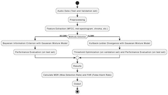
Figure 1. An overall framework of the study.

3.1. Task Definition

Given an audio signal S, the task of SCD is to find a set of change points for the segments, denoted as $Y=[y_1,\dots ,y_m]$, where $y_i\in {\mathbb{R}}^r$, r is the total number of frames in each window, and m is the total number of segments. Let $X_i={\left\{x_i\right\}}_{i=1}^n,x_i\in R^d$ represent the sequence of feature vectors of segment $y_i$, where $x_i$ is the features and n is the sample size, d is dimension of feature vector. Generally, speaker change point could be detected by calculating a distance or divergence between feature distributions of two adjacent audio segments and it can be represented as:

• a first segment of $X_i$ feature vector, the sequence of feature vectors from time $t_i$ to $t_{i+1}$.
• a second segment $X_{i+1}$, the sequence of feature vectors from time $t_{i+1}$ to $t_{i+2}$.

A speaker change is detected at time $t_{i+1}$ if the distance between these two segments exceeds a threshold $\tau$:

$$d\left(X_i,X_{i+1}\right)>\tau .$$

(1)

where d is a distance function, and $\tau$ is a threshold to detect changes in speaker.

3.2. Change Point Detection

In order to examine various features in a different settings, in this study, two methods are used for speaker change detection: Bayesian information criterion with Gaussian mixture model (BIC-GMM) and KL divergence with Gaussian mixture model (KL-GMM) method. BIC-GMM, which is based on model selection, and KL-GMM, which is metric-based.

3.2.1. BIC-GMM Method

This method uses the Bayesian information criterion to compare consecutive audio segments $X_i$ and $X_{i+1}$. It evaluates the following two hypotheses:

• $H_0$: both segments are derived from a Gaussian $\{X_i,X_{i+1}\}\sim N(\mu ,\Sigma )$ distribution, in other words, both segments belong to the same speaker.
• $H_1$: both segments are derived from two distinct Gaussians $X_i\sim N({\mu }_1,{\Sigma }_1)$ and $X_{i+1}\sim N({\mu }_2,{\Sigma }_2)$. The segments belong to different speakers.

With these hypotheses in mind, a BIC difference $\Delta BIC$ is calculated as:

$$\Delta BIC=(N_1+N_2)log|\Sigma |-N_{1}log|{\Sigma }_1|-N_{2}log\left|{\Sigma }_2\right|-\lambda P$$

(2)

$$P={\displaystyle \frac{1}{2}}\left(d+{\displaystyle \frac{1}{2}}d(d+1)\right)log\left(N\right)$$

(3)

where P is penalty term and $N=N_1+N_2$ are the sample sizes of the segments, and d is the dimension of the feature vector, and $\lambda$ is a penalty weight.

The larger value of $\Delta BI{C}_i$, the less similar the two segments are, indicating a greater distance between them. Instead of setting a threshold to it, we compare two $\Delta BI{C}_{i-1}$ value, if $\Delta BI{C}_i>\Delta BI{C}_{i-1}$, a change point is detected; otherwise, it is not.

3.2.2. KL Divergence

In this method, audio segments are modeled as Gaussian distributions. The KL divergence between two segments $X_i\sim N({\mu }_1,{\Sigma }_1)$ and $X_{i+1}\sim N({\mu }_2,{\Sigma }_2)$ is computed as:

$$D_{KL}(X_i\Vert X_{i+1})={\displaystyle \frac{1}{2}}\left(\mathrm{tr}\left({\Sigma }_2^{-1}{\Sigma }_1\right)+{({\mu }_2-{\mu }_1)}^T{\Sigma }_2^{-1}({\mu }_2-{\mu }_1)-d+log{\displaystyle \frac{|{\Sigma }_2|}{|{\Sigma }_1|}}\right)$$

(4)

where:

• $X_i,X_{i+1}$ represent two consecutive segments distributions.
• ${\mu }_1,{\mu }_2$ are mean vectors of the distributions $X_i$ and $X_{i+1}$, respectively.
• ${\Sigma }_1,{\Sigma }_2$ are covariance matrices of the distributions $X_i$ and $X_{i+1}$, respectively.
• $\mathrm{tr}\left({\Sigma }_2^{-1}{\Sigma }_1\right)$ represents the trace of the matrix product ${\Sigma }_2^{-1}{\Sigma }_1$, representing the sum of the eigenvalues of the product matrix.
• d is the dimensionality of the data or the number of features in $X_i$.

If KL difference is larger than the given threshold, it indicates a change point; otherwise, it does not. This approach requires specifically choosing the threshold value, as it is sensitive to this value. An inappropriate threshold may lead to either missed detections or false alarms, affecting the accuracy of change point detection.

3.3. Audio Features

As known, audio features play a vital role in the process of identifying change points. In order to analyze the different features, we choose different categories of feature based on their relevance to different aspects of the audio signal, can be summarized as follows:

• Mel-frequency cepstral coefficients (MFCC)—captures the timbral and phonetic content, which is useful for distinguishing different speakers.
• Mel-spectrogram—similar to the spectrogram but focused on the mel scale, which is more aligned with human hearing.
• Chroma—captures the harmonic content and pitch class, which can indicate tonal changes that may differentiate speakers.
• Spectral centroid—represents the “center of mass” of the spectrum, which often relates to the brightness of a sound.
• Spectral bandwidth—measures the spread of the spectrum, providing information about timbre and energy distribution.
• Spectral contrast—captures the difference between peaks and valleys in a spectrum, highlighting spectral variation which may signal speaker changes.
• Spectral rolloff—indicates the frequency below which a certain percentage of the total spectral energy is contained, useful for tracking energy shifts.
• Root mean square (RMS) energy—represents the power of the audio signal, which can help distinguish speakers based on loudness and energy pattern.
• Pitch—provides fundamental frequency information that can help differentiate speakers based on vocal pitch.
• Zero crossing rate—indicates the rate of signal sign changes, which can be useful for detecting changes in speech quality and distinguishing between different speakers.

Feature Changes vs. Speaker Changes

In the above we briefly describe each feature, in order to analyze those features how they useful to speaker change detection, the meetings audio from AMI corpus [31] is used in the following statistical counting. This section outlines the process of detecting changes in audio features and analyzing their co-occurrence with speaker changes.

By identifying points where specific features change (FC), we investigate how these changes align with speaker changes (SC) to inform feature selection for speaker change detection. For each audio feature, values are extracted over time, and points of significant change are identified by analyzing the differences between consecutive frames. This method accommodates both one-dimensional and two-dimensional feature data: (i) one-dimensional features (such as pitch) are straightforward; absolute differences between consecutive values are calculated to capture changes over time. (ii) two-dimensional features (such as MFCCs) involve multiple components per time frame. In this case, differences across dimensions are aggregated using the mean, which reflects overall changes in the feature values. Using the mean helps capture general trends across all components of a feature, making it suitable for analyzing broad patterns in audio data. Thresholds are applied to these feature differences to mark significant change points. By adjusting the threshold, it is possible to control the sensitivity of change detection for each feature.

After determining the change times for each feature, co-occurrence analysis is conducted to assess how often these feature changes align with speaker changes. A defined time window, set by the tolerance parameter, is used to determine if two events are co-occurred. A tolerance was set to 1 s, any feature change within this window of a speaker change is marked as a co-occurrence.

In the Figure 2, we plot thresholds against the probabilities $P\left(FC\right|SC)$ and $P\left(SC\right|FC)$, which represent the likelihood of feature changes given speaker changes, and vice versa, across various audio features.

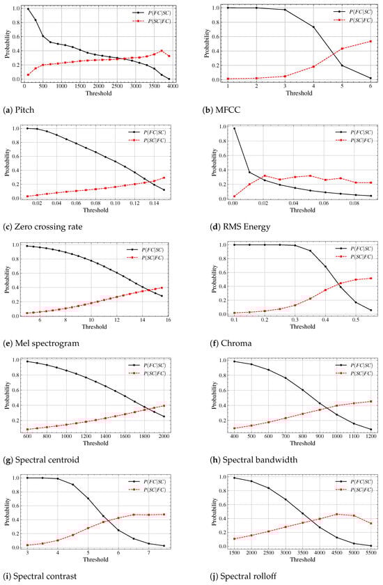
Figure 2. Probability distributions of speaker change (SC) and feature change (FC) across corresponding threshold values for various audio features.

Across all graphs, $P\left(FC\right|SC)$ generally starts at higher values at lower thresholds, indicating greater sensitivity to minor feature changes when a speaker change occurs. As thresholds increase, $P\left(FC\right|SC)$ gradually declines, indicating a reduction in sensitivity as the system filters out smaller changes. Conversely, $P\left(SC\right|FC)$ tends to rise as the threshold increases, indicating improved specificity. However, it does not reach unity (1) for any feature, meaning that even at high thresholds, the system does not perfectly align feature changes with speaker changes. However, no feature reaches unity (1) for $P\left(SC\right|FC)$, suggesting that even at high thresholds, the perfect alignment between feature changes and speaker changes is hard to be observed.

The intersection point of $P\left(SC\right|FC)$ and $P\left(FC\right|SC)$ can be observed in the Figure 2. These points represent the thresholds at which sensitivity and specificity are balanced, marking where the two probabilities are equal.

Table 1 provides the crossing points and the maximum observed $P\left(SC\right|FC)$ values for each feature. Crossing points where $P\left(FC\right|SC)$ and $P\left(SC\right|FC)$ intersect, and represent the thresholds at which sensitivity and specificity are balanced, marking where the two probabilities are equal. $P\left(SC\right|FC)$ value reflects the peak specificity that each feature achieves at a particular threshold, giving insights into how closely feature changes align with speaker changes. The highest values of $P\left(SC\right|FC)$ are observed for MFCC (0.534), chroma (0.515), pitch (0.40), and all the spectral related features have over 0.39 values. Other features, such as zero crossing rate and RMS energy, have lower maximum values around 0.32, indicating weaker alignment with speaker changes.

Table 1. Crossing points and the maximum values of $P\left(SC\right|FC)$ for various audio features.

Feature	Crossing Points	Max $\mathit{P}\left(\mathit{SC}\right|\mathit{FC})$
Pitch	0.2869	0.4008
MFCC	0.3153	0.5340
Zero crossing rate	0.2194	0.2931
RMS energy	0.2879	0.3196
Mel spectrogram	0.3614	0.3944
Chroma	0.4171	0.5149
Spectral centroid	0.3593	0.3941
Spectral bandwidth	0.3844	0.4521
Spectral contrast	0.4090	0.4746
Spectral rolloff	0.3332	0.4611

4. Experiments

In order to explore the effectiveness of different features and various distance metrics for SCD, we designed a set of experiments and report them in the following order:

(i) the threshold is a hyperparameter in metric-based SCD that determines the sensitivity of the detection process. This experiment seeks to effectively identify the optimal $\tau$ threshold for different feature and distance metric combinations on a subset of the validation set. (ii) considering a situation of imbalanced problem, the dataset may contains many negative samples, while only a small portion are positive samples. Under these conditions, a naive system that only outputs negative sample labels (in this case, 0) would achieve high accuracy but would fail to correctly identify positive samples. (iii) evaluate each combination of audio feature with different methods on the test data, and report the evaluation results. (iv) averaging the results for each method across all features to identify the most suitable features to SCD. (v) compare the empirically obtained results with the statistically obtained insights, and identifying the robust features by visualizing the comparison between the maximum probability of $P\left(SC\right|FC)$ and a combined score.

Robust features were clearly identified by visualizing the comparison between the maximum probability of $P\left(SC\right|FC)$ and the methods’ results. To effectively compare the metric-based approach, we designed an experiment using two naive systems as a baselines for comparisons.

4.1. Dataset and Evaluation Metric

Experiments were conducted using the AMI meeting corpus [31], a audio dataset commonly used for speech and audio processing research. The AMI corpus provided a diverse set of audio recordings that allowed us to evaluate the performance of these distance metrics under various conditions and scenarios. In the experiments, we used the standard validation and test split of the AMI corpus. The test data includes 16 meeting’s audios with a total duration of around 9 h, and an average duration of 33.38 min per meeting. The full data statistics are given in Table 2. It can be observed that the change points, overlaps, total number of speakers, and audio length are provided. For this statistic, 40% of the change points are overlapped.

Table 2. Dataset statistics: total change points, overlaps, speakers, and audio length. # represents the quantity of items.

Meeting ID	# Change Points	# Overlaps	% Overlaps	# Speakers	Length (min)
EN2002a	1366	678	49.63	4	43.90
EN2002b	954	444	46.55	4	33.52
EN2002c	1468	681	46.39	3	56.46
EN2002d	1331	662	49.74	4	46.02
ES2004a	360	145	40.28	4	15.71
ES2004b	687	257	37.41	4	37.48
ES2004c	722	262	36.29	4	37.71
ES2004d	893	351	39.31	4	34.02
IS1009a	290	122	42.07	4	11.91
IS1009b	602	251	41.70	4	33.24
IS1009c	494	142	28.74	4	26.51
IS1009d	688	245	35.61	4	29.27
TS3003a	424	95	22.41	4	17.54
TS3003b	658	157	23.86	4	30.63
TS3003c	629	160	25.44	4	31.83
TS3003d	1061	345	32.52	4	35.16
Total	13,127	5253	40.02	-	548.70
Average	821.31	328.19	37.57	3.94	33.38

In the preprocessing step, 1-second chunk presegmentation was applied before the experiments. All audio files were then resampled to 16 kHz, and the following parameter settings were used for feature extraction: $hop\_length=512$ and $n\_fft=2048$.

For evaluation, the following metrics were chosen for the comparative analysis. False alarm rate (FAR) indicates the frequency of incorrect detections of speaker changes. It is calculated as the proportion of false positives (FP) among all non-change points:

$$\mathrm{FAR}={\displaystyle \frac{\mathrm{False}\mathrm{positives}\left(\mathrm{FP}\right)}{\mathrm{False}\mathrm{positives}\left(\mathrm{FP}\right)+\mathrm{True}\mathrm{negatives}\left(\mathrm{TN}\right)}}$$

(5)

Missed detection rate (MDR) measures how often the system fails to detect an actual speaker change. It is the proportion of false negatives (FN) among all true change points:

$$\mathrm{MDR}={\displaystyle \frac{\mathrm{False}\mathrm{negatives}\left(\mathrm{FN}\right)}{\mathrm{True}\mathrm{positives}\left(\mathrm{TP}\right)+\mathrm{False}\mathrm{negatives}\left(\mathrm{FN}\right)}}$$

(6)

$$\mathrm{Performance}\mathrm{Score}=1-{\displaystyle \frac{\mathrm{FAR}+\mathrm{MDR}}{2}}$$

(7)

Performance score reflects both types of errors (false alarm rate and missed detection rate), this score is only used for threshold optimization.

4.2. Experimental Setup

To conduct a fair and comparable experiments, we define the following points: (i) choose 16 kHz as the main sample rate of audios; (ii) set parameter of hop length to 512 and n_fft set to 2048 for extracting the audio feature from raw signals. Each meeting was segmented to short 1s audio, before extracting the features.

Since the true labels of speaker change points are given as timestamps on the raw audio signal, such as beginning time, we match this beginning times for obtain the labels for each segment. The test set was used solely for final evaluation, guaranteeing that the chosen thresholds are fair, as they are not influenced by direct tuning on the test data. Validation set was used for threshold optimization for KL divergence with GMM. For simplicity, in the experiments, we refer to the method of KL-divergence with GMM as KL-GMM. BIC-GMM models are simplified to BIC.

4.3. Results

In the threshold optimization process for SCD, Bayesian optimization was applied to determine the optimal threshold for each combination of audio feature for KL-GMM, with the aim of maximizing the performance score on the validation set. The optimization process is configured with the following parameters:

• Threshold parameter is explored within the range of 0 to 10, allowing the optimizer to identify both highly sensitive and more robust threshold values across various feature and metric combinations.
• Initialization points set to 5, this parameter specifies the number of random points the optimizer initially samples to gain a broad understanding of the threshold’s impact on the combined metric as peformance score.
• Iterations set to 25, this parameter specifies the number of optimization steps following the initial exploration.

The process begins with a set number of random samples, after which the optimizer uses these observations to inform subsequent iterations. B focusing on the most promising thresholds, Bayesian optimization quickly converges on the values that maximize the performance score. It is shown in Figure 3, the fluctuation is process of optimization, and with the blue cure, the convergence curve with performance score is plotted. The final optimized threshold values are list in Table 3.

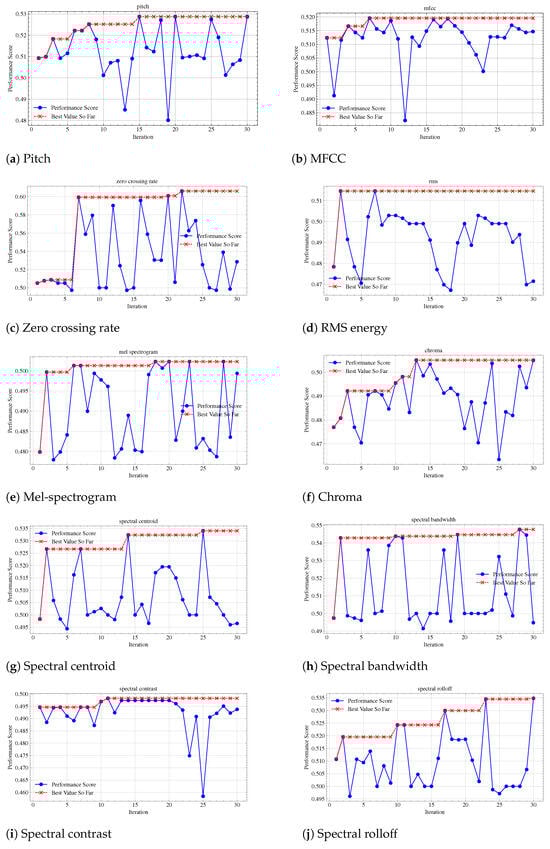
Figure 3. Threshold optimization with Bayesian approach for KL divergence on validation set.

Table 3. Optimal thresholds of KL divergence method for each feature after optimized on validation set with Bayesian optimization.

Feature	Optimal Threshold	Performance Score
Pitch	5.999179	0.528707
MFCC	4.331410	0.519567
Chroma	9.998953	0.505080
Mel-spectrogram	0.604765	0.502307
Zero crossing rate	0.988847	0.606065
Spectral centroid	0.441515	0.534054
Spectral bandwidth	0.763678	0.547675
Spectral contrast	4.665370	0.498247
Spectral rolloff	0.539069	0.534808
RMS energy	0.259262	0.514598

Two naive systems considered as baselines for comparison, they are (i) ${\mathrm{naive}}_0$: it is only output 0 (negative) label. (ii) ${\mathrm{naive}}_1$: the system only output 1 (positive) label. Table 4 lists the FAR and MDR for the naive systems, which are shown here for comparison purposes with the KL-GMM and BIC-GMM.

Table 4. Results of naive systems for comparison.

	FAR	MDR
${\mathrm{naive}}_0$	0	1
${\mathrm{naive}}_1$	1	0

Table A1, Table A2, Table A3, Table A4, Table A5, Table A6, Table A7, Table A8, Table A9 and Table A10 lists the detailed results of two approaches across different features: Chroma, Mel-spectrogram, MFCC, Pitch, RMS energy, Spectral bandwidth, Spectral centroid, Spectral contrast, Spectral rolloff, and Zero crossing rate for different meeting records.

First of all, compared to the naive systems, both KL-GMM and BIC-GMM that processing the audio features, doing a real detection of speaker changes. They reduce the errors found in naive systems by analyzing the audio, rather than relying on fixed assumptions.

It can be seen from Figure 3d,e, although the threshold of KL-GMM with Mel-spectrogram (Table A2) feature and RMS energy feature (Table A5) was optimized for the validation set well, but on the test data, it produces extremely high FAR values (close to 1.0) but very low MDR values, indicating that it detects almost all change points, but at the cost of many false alarms. In this case, the performance of the KL-GMM is similar to the ${\mathrm{naive}}_1$ system due to improper threshold values. KL-GMM with the pitch (Table A4) feature gives a high MDR value and a low FAR. In this situation, it behaves similarly to the ${\mathrm{naive}}_0$ system, but slightly better.

However, KL-GMM as a sensitive method to threshold, with feature MFCC (Table A3), and Zero cross rate feature (Table A10) shows a balanced result with FAR and MDR across different meeting test sets. This reflects the fact that optimizing a threshold value for KL divergence is challenging and may not always work well across different audio data. Variations in audio signals, such as slight environmental changes or differences in speaker characteristics, can lead to significant changes in feature values, causing the method to fail in detecting speaker changes. BIC-GMM appears less influenced by variability of different feature value, it achieves more stable performance across different meetings. It also maintains more balanced FAR and MDR rates across all features.

Table 5 reports the average results of meetings for different features. It can be observed that the lowest MDR value of 44.99% was achieved by BIC-GMM with the MFCC feature, with a corresponding FAR of 48.37%. KL-GMM with the MFCC feature gave an MDR of 46.71% and an FAR of 54.28%, which is considered a good performance compared to other features. These results indicate that MFCC features is good fit to SCD problem when using KL and BIC techniques. Additionally, the conditional probability of speaker change given a feature change, $P{\left(SC\right|FC)}_{MFCC}$, is 53.40% for the MFCC feature (see Table 1). This value aligns with the experimental result for both BIC-GMM and KL-GMM with MFCC feature. The conditional probability for the Chroma feature, $P{\left(SC\right|FC)}_{Chroma}$, is 51.49%, showing a similar pattern.

Table 5. Average SCD results for KL-GMM and BIC-GMM across features.

Feature	FAR (KL)	MDR (KL)	FAR (BIC)	MDR (BIC)
Chroma	0.2889	0.6941	0.4911	0.4716
Mel-spectrogram	0.9927	0.0062	0.5034	0.5128
MFCC	0.5428	0.4671	0.4837	0.4499
Pitch	0.1470	0.8508	0.4947	0.4894
RMS energy	0.8809	0.1300	0.4817	0.4720
Spectral bandwidth	0.5948	0.3869	0.4938	0.4700
Spectral centroid	0.7606	0.2299	0.4882	0.4690
Spectral contrast	0.0975	0.9009	0.4855	0.4653
Spectral rolloff	0.7667	0.2318	0.4890	0.4774
Zero crossing rate	0.5061	0.4827	0.4968	0.4928
Average	0.5578	0.4380	0.4908	0.4770
Standard Deviation	0.2919	0.2899	0.0110	0.0292

When we calculate the standard deviation for KL divergence and BIC-GMM model, it can be observed that, for KL divergence (0.29 for FAR, 0.28 for MDR), its std values are much higher than BIC-GMM’s (0.011 for FAR, 0.029 for MDR). This indicates that the BIC-GMM model has more consistent performance across different instances, with lower variability in both FAR and MDR. In contrast, the higher standard deviation values for KL divergence suggest that its performance fluctuates more depending on the specific audio data and conditions.

Figure 4 presents the relation between maximum probability of speaker change given feature change Max$P\left(SC\right|FC)$ with the FAR and MDR results for BIC-GMM and KL-GMM. To compare different features, we need to compare both MDR and FAR value in a balanced way. For example, in BIC-GMM with feature RMS (see Figure 4a,b), its FAR value is lowest among others, but it has high MDR.

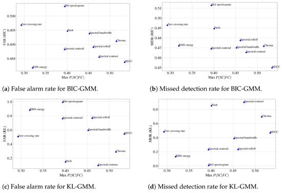
Figure 4. Relation between Max$P\left(SC\right|FC)$ with results of BIC-GMM (the lower value is good).

It can be observed that for MFCC in BIC-GMM (see Figure 4a,b), the highest probability of $P\left(SC\right|FC)$ corresponds to the lowest MDR and FAR values. It shows Mel-spectrogram has the highest value for both MDR and FAR scores in BIC-GMM (see Figure 4a,b) It may indicate it is not suits to the SCD compared to others.

To clearly demonstrate the effectiveness of different features on two distinct methods, we use a combined score of MDR and FAR by approximating the F1 score:

$$\mathrm{Approx}.\mathrm{F}1\approx 2\times {\displaystyle \frac{(1-\mathrm{FAR})\times (1-\mathrm{MDR})}{(1-\mathrm{FAR})+(1-\mathrm{MDR})}}$$

(8)

Figure 5 compares the performance of various audio features across two speaker change detection methods: KL-GMM and BIC-GMM, using approx. F1 scores, and shows the relation with Max$P\left(SC\right|FC)$. In both methods, MFCC achieving the highest approx. F1 score, which indicates effective detection with a balanced reduction in both false alarms and missed detection. Correspondingly, its Max$P\left(SC\right|FC)$ value is also the highest.

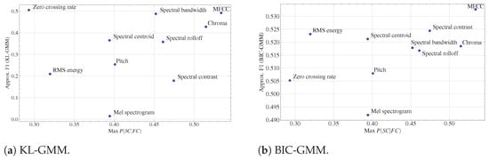
Figure 5. Relation between Max$P\left(SC\right|FC)$ vs. $\mathrm{Approx}.\mathrm{F}1\mathrm{score}$ (the higher value is good).

BIC-GMM method demonstrates more consistent approx. F1 scores across features, with RMS energy, spectral centroid, Spectral bandwidth, and Chroma all performing reasonably well. Zero crossing rate ranks highest for KL-GMM, with an approx. F1 and a relatively low Max$P\left(SC\right|FC)$ value. However, this feature did not outperform others in BIC-GMM (Figure 5b), except for Mel-spectrogram feature that consistently underperforms across both methods, although it shows slightly improved performance in BIC-GMM.

5. Conclusions

In this paper, an empirical comparative study using various audio features with different methods for unsupervised SCD is presented. A various of audio features were evaluated for two methods: BIC-GMM and KL divergence with GMM, the former approach is no need threshold optimization, but the latter does. Various features were experimented such as MFCC, mel-spectrogram, spectral centroid, spectral bandwidth, spectral contrast, spectral rolloff, RMS, pitch, zero crossing rate. In order to gain insight into which features have a significant impact on the SCD problem, two conditional distributions from a corpus, such as the probability of feature change given a speaker change $P\left(FC\right|SC)$ and the probability of speaker change given feature change were calculated. Crossing points between these two probabilities and the maximum $P\left(SC\right|FC)$ for each features were calculated. The crossing points represent the thresholds at which sensitivity and specificity are balanced, marking where the two probabilities are equal. The maximum $P\left(SC\right|FC)$ giving insights how closely feature changes align with speaker changes.

Different experiments were carried out for comparing the combinations of method across features: (i) the threshold was optimized on the validation set for KL-GMM approach using Bayesian optimization process. (ii) results for two naive systems were reported as baseline considering the situation of unbalanced class of SCD. (iii) evaluate each combination of audio feature with different methods on the test data, and report the evaluation results. (iv) averaging the results for each method across all features to identify the most suitable features to SCD.

For evaluation, false alarm rate and missed detection rate were calculated. Experimental results can be summarized as follows:

(i)

For different features, KL-GMM approache using Bayesian optimization process to find optimal threshold value on the validation set and the optimal value with the optimization process was reported.

(ii)

Comparing with two naive systems, both KL-GMM and BIC-GMM that processing the audio features, doing a real detection of speaker changes.

(iii)

KL-GMM peformance with some feature combination similar to two naive systems, like giving extreme high value to FAR or low value to MDR, vice versa. Although, the thresholds are well optimized on the validation set, it still fails to handle the variability of new audio dataset. KL-GMM as a sensitive mehtod to threshold, but with features like MFCC and zero cross rate shows a better performance. BIC-GMM showed a robust performance on handling the variability of different feature values compared it with KL-GMM, and it achieves more stable performance across different meetings.

(iv)

Average results indicate that both BIC-GMM and KL-GMM perform effectively on the SCD when using MFCC features. This suggests that MFCC features are well-suited for SCD with these techniques. With the highest $P\left(SC\right|FC)$ value, MFCC, also has the lowest MDR and FAR, confirming the expectations derived from the statistics.

(v)

The relation between Max$P\left(SC\right|FC)$ vs approx. F1 score showed that MFCC consistently ranks high across both methods, confirming its effectiveness. Zero crossing rate, Chroma and Spectral contrast gives a higher performance in BIC-GMM. Mel-spectrogram consistently ranks at the bottom, suggesting it has the least impact on performance across both methods.

The potential future work can be summarized as follows: (i) applying deep learning methods and comparing their results with those obtained using traditional MFCC features; (ii) exploring the use of pre-trained large audio models for the SCD task; (iii) investigating a multi-modal SCD approach that combines audio signal data with its transcription, leveraging both large audio models and large language models

References

- Anguera, X.; Bozonnet, S.; Evans, N.; Fredouille, C.; Friedland, G.; Vinyals, O. Speaker Diarization: A Review of Recent Research. IEEE Trans. Audio Speech Lang. Process. 2012, 20, 356–370. [Google Scholar] [CrossRef]
- Tranter, S.; Reynolds, D.A. An overview of automatic speaker diarization systems. IEEE Trans. Audio Speech Lang. Process. 2006, 14, 1557–1565. [Google Scholar] [CrossRef]
- Tranter, S.E.; Evermann, G.; Kim, D.Y.; Woodland, P.C. An Investigation into the Interactions between Speaker DiarisationSystems and Automatic Speech Transcription B Accuracy of Cts Forced Alignments 44; Cambridge University Engineering Department: Cambridge, UK, 2003. [Google Scholar]
- Aronowitz, H.; Burshtein, D.; Amir, A. Speaker Indexing in Audio Archives Using Gaussian Mixture Scoring Simulation. In Machine Learning for Multimodal Interaction, Proceedings of the First International Workshop, MLMI 2004, Martigny, Switzerland, 21–23 June 2004; Bengio, S., Bourlard, H., Eds.; Springer: Berlin/Heidelberg, Germany, 2005; pp. 243–252. [Google Scholar]
- Chen, S.; Gopalakrishnan, P.S.; Watson, I.T.J. Speaker, Environment and Channel Change Detection and Clustering via the Bayesian Information Criterion. In Proceedings of the DARPA Broadcast News Transcription and Understanding Workshop, Lansdowne, Virginia, 8–11 February 1998. [Google Scholar]
- Siegler, M.A.; Jain, U.; Raj, B.; Stern, R.M. Automatic Segmentation, Classification and Clustering of Broadcast News Audio. In Proceedings of the DARPA Speech Recognition Workshop, Chantilly, VA, USA, 24 December 1997. [Google Scholar]
- Gish, H.; Siu, M.H.; Rohlicek, R. Segregation of speakers for speech recognition and speaker identification. In Proceedings of the ICASSP 91: 1991 International Conference on Acoustics, Speech, and Signal Processing, Toronto, ON, Canada, 14–17 April 1991; Volume 2, pp. 873–876. [Google Scholar] [CrossRef]
- Bonastre, J.F.; Delacourt, P.; Fredouille, C.; Merlin, T.; Wellekens, C. A speaker tracking system based on speaker turn detection for NIST evaluation. In Proceedings of the 2000 IEEE International Conference on Acoustics, Speech, and Signal Processing, Istanbul, Turkey, 5–9 June 2000; Volume 2, pp. II1177–II1180. [Google Scholar] [CrossRef]
- Malegaonkar, A.; Ariyaeeinia, A.; Sivakumaran, P.; Fortuna, J. Unsupervised speaker change detection using probabilistic pattern matching. IEEE Signal Process. Lett. 2006, 13, 509–512. [Google Scholar] [CrossRef]
- Ajmera, J.; McCowan, I.; Bourlard, H. Robust speaker change detection. IEEE Signal Process. Lett. 2004, 11, 649–651. [Google Scholar] [CrossRef]
- Dehak, N.; Kenny, P.J.; Dehak, R.; Dumouchel, P.; Ouellet, P. Front-End Factor Analysis for Speaker Verification. IEEE Trans. Audio Speech Lang. Process. 2011, 19, 788–798. [Google Scholar] [CrossRef]
- Snyder, D.; Garcia-Romero, D.; Sell, G.; Povey, D.; Khudanpur, S. X-Vectors: Robust DNN Embeddings for Speaker Recognition. In Proceedings of the 2018 IEEE International Conference on Acoustics, Speech and Signal Processing (ICASSP), Calgary, AB, Canada, 15–20 April 2018; pp. 5329–5333. [Google Scholar]
- Variani, E.; Lei, X.; McDermott, E.; López-Moreno, I.; Gonzalez-Dominguez, J. Deep neural networks for small footprint text-dependent speaker verification. In Proceedings of the 2014 IEEE International Conference on Acoustics, Speech and Signal Processing (ICASSP), Florence, Italy, 4–9 May 2014; pp. 4052–4056. [Google Scholar]
- Mukhamediev, R.I.; Popova, Y.; Kuchin, Y.; Zaitseva, E.; Kalimoldayev, A.; Symagulov, A.; Levashenko, V.; Abdoldina, F.; Gopejenko, V.; Yakunin, K.; et al. Review of Artificial Intelligence and Machine Learning Technologies: Classification, Restrictions, Opportunities and Challenges. Mathematics 2022, 10, 2552. [Google Scholar] [CrossRef]
- Sinha, R.; Tranter, S.E.; Gales, M.J.F.; Woodland, P.C. The Cambridge University March 2005 speaker diarisation system. In Proceedings of the 9th European Conference on Speech Communication and Technology, Lisbon, Portugal, 4–8 September 2005; pp. 2437–2440. [Google Scholar] [CrossRef]
- Wang, D.; Lu, L.; Zhang, H.J. Speech segmentation without speech recognition. In Proceedings of the 2003 International Conference on Multimedia and Expo, ICME ’03, Proceedings (Cat. No.03TH8698), Baltimore, MD, USA, 6–9 July 2003; Volume 1, pp. 1–405. [Google Scholar] [CrossRef]
- Lu, L.; Zhang, H.J.; Jiang, H. Content analysis for audio classification and segmentation. IEEE Trans. Speech Audio Process. 2002, 10, 504–516. [Google Scholar] [CrossRef]
- Toleu, A.; Tolegen, G.; Mussabayev, R.; Zhumazhanov, B.; Krassovitskiy, A. Comparative Analysis of Distance Measures for Unsupervised Speaker Change Detection. In Proceedings of the 2024 20th International Asian School-Seminar on Optimization Problems of Complex Systems (OPCS), Novosibirsk, Russian Federation, 19–30 July 2024; pp. 28–32. [Google Scholar] [CrossRef]
- Desplanques, B.; Demuynck, K.; Martens, J.P. Factor analysis for speaker segmentation and improved speaker diarization. In Proceedings of the 16th Annual Conference of the International Speech Communication Association (Interspeech 2015), Dresden, Germany, 6–10 September 2015. [Google Scholar]
- Neri, L.V.; Pinheiro, H.N.; Tsang, I.R.; da C. Cavalcanti, G.D.; Adami, A.G. Speaker segmentation using i-vector in meetings domain. In Proceedings of the 2017 IEEE International Conference on Acoustics, Speech and Signal Processing (ICASSP), New Orleans, LA, USA, 5–9 March 2017; pp. 5455–5459. [Google Scholar] [CrossRef]
- Sarkar, A.; Dasgupta, S.; Naskar, S.K.; Bandyopadhyay, S. Says Who? Deep Learning Models for Joint Speech Recognition, Segmentation and Diarization. In Proceedings of the 2018 IEEE International Conference on Acoustics, Speech and Signal Processing (ICASSP), Calgary, AB, Canada, 15–20 April 2018; pp. 5229–5233. [Google Scholar]
- Wang, R.; Gu, M.; Li, L.; Xu, M.; Zheng, T.F. Speaker segmentation using deep speaker vectors for fast speaker change scenarios. In Proceedings of the 2017 IEEE International Conference on Acoustics, Speech and Signal Processing (ICASSP), New Orleans, LA, USA, 5–9 March 2017; pp. 5420–5424. [Google Scholar] [CrossRef]
- Zhang, A.; Wang, Q.; Zhu, Z.; Paisley, J.W.; Wang, C. Fully Supervised Speaker Diarization. In Proceedings of the ICASSP 2019—2019 IEEE International Conference on Acoustics, Speech and Signal Processing (ICASSP), Brighton, UK, 12–17 May 2018; pp. 6301–6305. [Google Scholar]
- Jati, A.; Georgiou, P. Speaker2Vec: Unsupervised Learning and Adaptation of a Speaker Manifold Using Deep Neural Networks with an Evaluation on Speaker Segmentation. In Proceedings of the Interspeech 2017, Stockholm, Sweden, 20–24 August 2017; pp. 3567–3571. [Google Scholar] [CrossRef]
- Sivakumaran, P.; Fortuna, J.; Ariyaeeinia, A.M. On the use of the Bayesian information criterion in multiple speaker detection. In Proceedings of the Interspeech, Aalborg, Denmark, 3–7 September 2001. [Google Scholar]
- Malegaonkar, A.S.; Ariyaeeinia, A.M.; Sivakumaran, P. Efficient Speaker Change Detection Using Adapted Gaussian Mixture Models. IEEE Trans. Audio Speech Lang. Process. 2007, 15, 1859–1869. [Google Scholar] [CrossRef]
- Meignier, S.; Bonastre, J.F.; Igounet, S. E-HMM approach for learning and adapting sound models for speaker indexing. In Proceedings of the ISCA, a Speaker Odyssey, the Speaker Recognition Workshop, Chiana, Greece, 18–22 June 2001; p. 5. [Google Scholar]
- Gupta, V. Speaker change point detection using deep neural nets. In Proceedings of the 2015 IEEE International Conference on Acoustics, Speech and Signal Processing (ICASSP), South Brisbane, Australia, 19–24 April 2015; pp. 4420–4424. [Google Scholar] [CrossRef]
- Hrúz, M.; Zajíc, Z. Convolutional neural network for speaker change detection in telephone speaker diarization system. In Proceedings of the 2017 IEEE International Conference on Acoustics, Speech and Signal Processing (ICASSP), New Orleans, LA, USA, 5–9 March 2017. [Google Scholar]
- Hrúz, M.; Hlaváč, M. LSTM Neural Network for Speaker Change Detection in Telephone Conversations. In Speech and Computer, Proceedings of the 20th International Conference, SPECOM 2018, Leipzig, Germany, 18–22 September 2018; Karpov, A., Jokisch, O., Potapova, R., Eds.; Springer: Cham, Switzerland, 2018; pp. 226–233. [Google Scholar]
- Carletta, J.; Ashby, S.; Bourban, S.; Flynn, M.; Guillemot, M.; Hain, T.; Kadlec, J.; Karaiskos, V.; Kraaij, W.; Kronenthal, M.; et al. The AMI Meeting Corpus: A Pre-Announcement. In Machine Learning for Multimodal Interaction, Proceedings of the Second International Workshop, MLMI 2005, Edinburgh, UK, 11–13 July 2005; Springer: Berlin/Heidelberg, Germany, 2005; pp. 25–29. [Google Scholar]
Disclaimer/Publisher’s Note: The statements, opinions and data contained in all publications are solely those of the individual author(s) and contributor(s) and not of MDPI and/or the editor(s). MDPI and/or the editor(s) disclaim responsibility for any injury to people or property resulting from any ideas, methods, instructions or products referred to in the content. |
© 2024 by the authors. Licensee MDPI, Basel, Switzerland. This article is an open access article distributed under the terms and conditions of the Creative Commons Attribution (CC BY) license (https://creativecommons.org/licenses/by/4.0/).