Bayesian Optimization for Instruction Generation

Abstract

The performance of Large Language Models (LLMs) strongly depends on the selection of the best instructions for different downstream tasks, especially in the case of black-box LLMs. This study introduces BOInG (Bayesian Optimization for Instruction Generation), a method leveraging Bayesian Optimization (BO) to efficiently generate instructions while addressing the combinatorial nature of instruction search. Over the last decade, BO has emerged as a highly effective optimization method in various domains due to its flexibility and sample efficiency. At its core, BOInG employs Bayesian search in a low-dimensional continuous space, projecting solutions into a high-dimensional token embedding space to retrieve discrete tokens. These tokens act as seeds for the generation of human-readable, task-relevant instructions. Experimental results demonstrate that BOInG achieves comparable or superior performance to state-of-the-art methods, such as InstructZero and Instinct, with substantially lower resource requirements while also enabling the use of both white-box and black-box models. This approach offers both theoretical and practical benefits without requiring specialized hardware.

1. Introduction

Large Language Models (LLMs) have triggered an amazing amount of innovation in several domains of the machine learning arena. In this paper, we focus on the design of experiments and black-box optimization, which have not been extensively explored to date, despite the integration of LLMs and optimization, which present many opportunities. Foundational language models can be game changers in optimization, leveraging the enormous amount of information available in free-form text an entirely new approach to optimization task comprehension, exploiting wider contexts across new tasks and generalizing pre-trained models over unseen search spaces.

The considerations outlined in the Introduction were inspired by [1], which argues the potential of foundational models for enhancing black-box optimization and advocates for the adoption of transformers and LLMs to achieve this goal.

A general approach is proposed in [2] that introduces LLMs as optimizers, describing the optimization task through natural language. In each optimization step, the LLM generates new solutions from the prompts that contain the previously generated solutions with their values. The first problems considered are linear regression and the travelling salesman problem, with prompt optimization aimed at finding instructions that maximize the task-specific objective function. In [3], it is demonstrated that, using textual representations of mathematical values, LLMs can act as universal regressors. The proposed method, namely OmniPred, can take as input dynamically varying input spaces and does not require normalization. LLMs can also be used in the framework of evolutionary optimization [4] for single-objective and multi-objective evolutionary optimization [5,6].

Another computational framework for exploiting LLMs in black-box optimization is Bayesian Optimization (BO) [7]. The potential of the transformer architecture for Bayesian inference was represented in [8] with respect to In-Context Learning (ICL). More recently, in [9], it was shown how to frame the basic BO algorithm [10,11] in natural language terms, enabling LLMs to sequentially propose promising solutions conditioned on previous trials and observations. The proposed approach, namely LLAMBO (Large Language Model for Bayesian Optimization), addresses two critical problems: enhancing, through LLMs, the key components of BO, including the surrogate model and the acquisition function, and leveraging modules of different processes in the BO pipeline in natural language terms. In the basic BO algorithm and most of its extensions, the Gaussian Process (GP) [12,13] is the most common choice for the probabilistic surrogate model. Other methods have been attracting increasing attention. It is well known that neural networks are universal approximators, as the GP has key advantages of an analytical formula and a principled estimate of the uncertainty. On the other hand, neural networks, especially Bayesian Neural Networks (BNNs), have been also considered due to their flexibility in handling high-dimensional optimization problems. Moreover, the availability of computing power has brought to the fore the use of Monte Carlo methods for estimating uncertainty. Finally, transformers can provide another surrogate model with an advantage over the GP of integrating naturally contextual understanding, few-shot learning, and domain knowledge.

The relation between LLMs and BO is two-way: along with the role of LLMs in enhancing Bayesian optimization, another line is to exploit BO to improve prompt/instruction engineering to enable LLMs to solve a specific task. The focus in this paper is on the second objective, analyzing recent BO methods and proposing a new and less resource-consuming approach.

1.1. Organization of the Paper

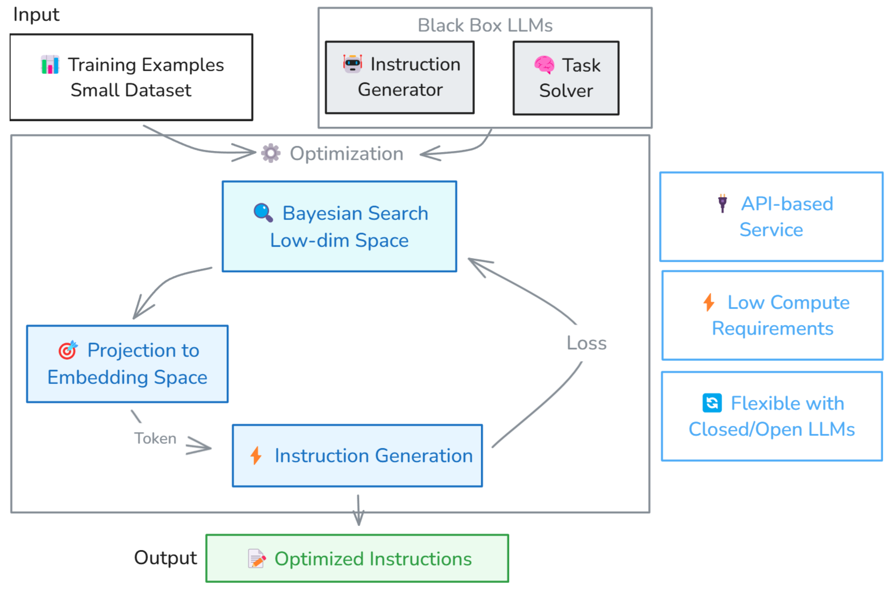
Section 2 provides a synthetic reference to the main approaches for prompt/instruction optimization. Section 3 details the approach proposed in this paper, namely BOInG (Bayesian Optimization for Instruction Generation) (Figure 1). Section 4 provides the experimental settings and the results. Section 5 provides concluding remarks on, limitations of, and perspectives of BOInG and, more generally, BO in working with LLMs.

Figure 1. High-level BOInG instruction generation workflow and components.

1.2. Contributions

Form the methodological point of view, a new strategy is proposed to deal with the combinatorial nature of the problem. Instead, of performing BO in low-dimensional continuous space, then trying to recast the solution to the closest possible text, a penalty is included in the BO acquisition function to push the search for promising solutions towards low-dimensional representations of texts known to the LLMs.

As most of current approaches, BOInG works with two LLMs, with the first used as an instructor generator and the second used as a solver for a specific task. While other state-of-the art approaches–discussed in the following subsection “related works”–require that at least one of the two LLMs is a white-box model, in BOInG, both the LLMs can be black-box models, leading to a significant reduction in computational resource use “on premises”. BOInG overcomes these limitations by leveraging two black-box LLMs, currently implemented with GPT-3.5 but extensible to more advanced closed-source models like GPT-4o. This is particularly advantageous, as the highest-performing models are often closed-source, while open-source alternatives typically offer lower quality and require larger architectures to achieve comparable results, further increasing computational demands and necessitating multi-GPU setups. BOInG accesses these models via an API in an “as-a-service” paradigm, only requiring the embedding of a white-box LLM (specifically, GPT-2) for penalty computation to apply to the acquisition function. By eliminating the need to run the full LLM locally, BOInG substantially reduces computational requirements while maintaining the optimization paradigm.

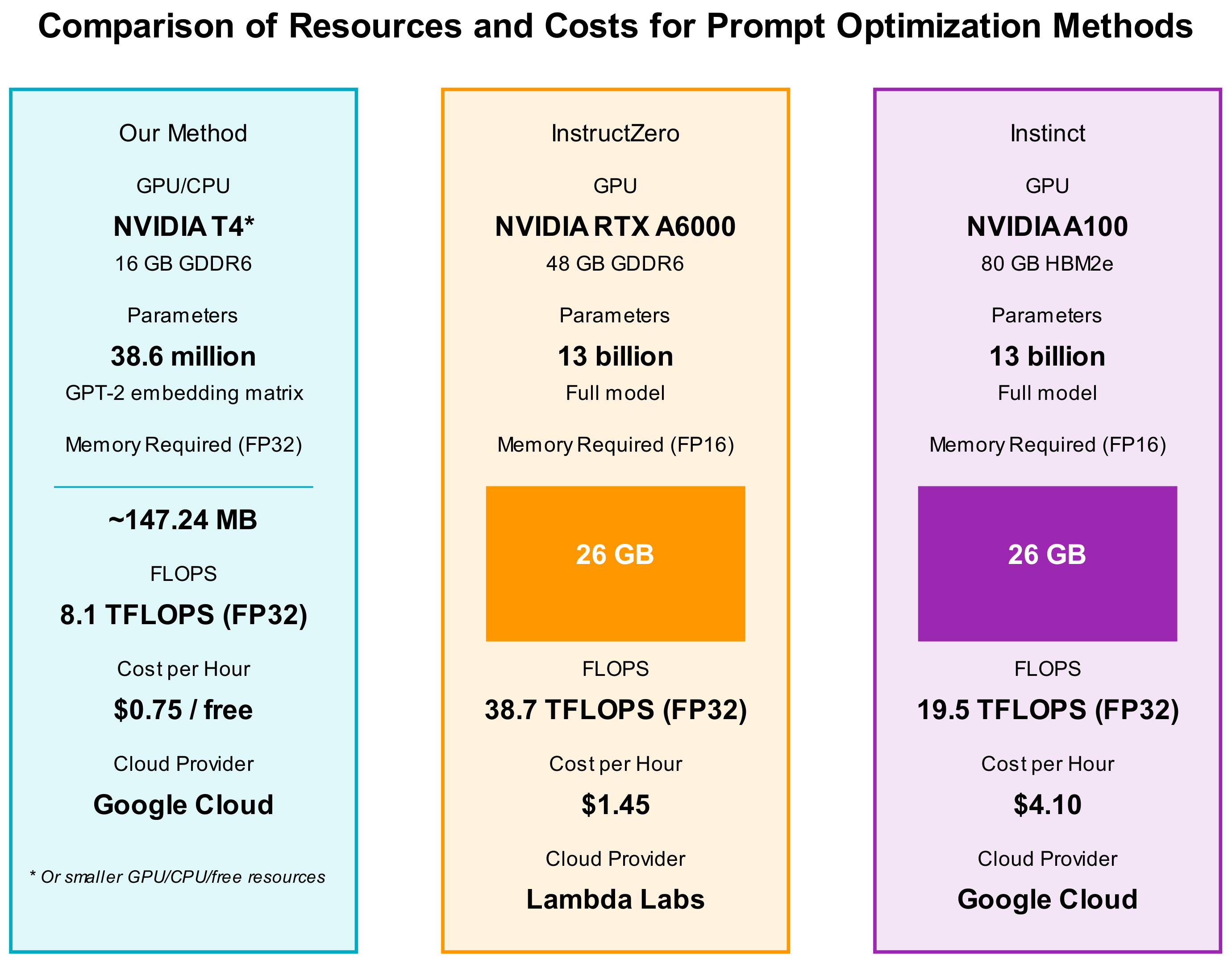
Figure 2 summarizes the costs of BOInG against those of two state-of-the-art methods, namely InstructZero [14] and Instinct [15], as described in the following.

Figure 2. Comparison of computational resources and costs across three BO-based instruction generation approaches. Information is related to the GPU type, parameter count, memory needed, FLOPS, hourly cost, and cloud provider for BOInG, InstructZero, and Instinct. It is evident that BOInG uses significantly fewer parameters and requires significantly less memory.

2. Related Works

In [16], a prompt ($\mathbf{p}\in V^l$) is defined as a sequence of $l$ n-grams. The tokens of the original model’s vocabulary are merged in n-grams based on their Pointwise Mutual Information (PMI) and considered as prompt candidates. This ensures that only n-grams of tokens that frequently appear together are used to form the actual vocabulary (V).

The final goal is to find the prompt (${\mathbf{p}}^{\mathbf{\ast }}$) that maximizes a scoring function ($h$). The scoring function ($h$) utilized in the prompt optimization framework is defined as the classification score between the predicted label and the ground-truth label. The algorithm proposed in [16] is analyzed is Section 4; it is based on vanilla BO over a continuous relaxation of the combinatorial space and a successive rounding of the continuous solution to the closest integer-valued solution.

On the contrary, InstructZero [14] deals with discrete instructions by optimizing over a low-dimensional continuous latent space and using a linear projection to map the result back to the original discrete space. The soft prompt in the continuous latent space is given as input to an open-source LLM whose output is an instruction which, in turn, is given a black-box LLM as input. BO is used to identify new soft prompts aimed at improving the zero-shot performance.

Another approach using two LLMs is named Instinct [15], which moves from the observation that gaussian processes (GPs), which are usually adopted as probabilistic surrogate models in BO, perform poorly for sophisticated or high-dimensional objective functions. This can become a serious drawback attributed to the representational power of GPs, which are usually unsuitable when a soft prompt is the argument of the mapping. Owing to this drawback, growing attention is being paid to transformer architectures, which have empirically shown not only a better representation capacity but also effectiveness in balancing exploration and exploitation, in alignment with GPs.

The method proposed in this paper is called BOInG (Bayesian Optimization for Instruction Generation), and it is also based on two LLMs: one used as an instruction generator and the other used as a solver of the target task. In contrast to InstructZero and Instinct, in which one LLM must be a white-box model, in BOING, both LLMs can be black-box models.

2.1. Common Background and Notation

A prompt ($\mathbf{p}$) is a sequence of a given length ($L$) of n-grams or of individual tokens selected from a vocabulary ($V$). The goal is to engineer prompts to address a specific task with an input space ($\mathcal{X}$) and an output defined as $f\left(\mathbf{p},\mathbf{X}\right)$, where $\mathbf{X}\in \mathcal{X}$. Usually, a query ($\mathbf{q}$) is denoted as $concatenate\left(\mathbf{p},\mathbf{X}\right)$.

The generation of the most suitable prompt for a given task is formulated as an optimization problem with an objective function that measures the performance on a given task, that is, $h\left(f\left(\mathbf{p},\mathbf{X}\right),\mathbf{Y}\right)$. Common choices for the score function are evaluation metrics such as accuracy or F1 for classification tasks and mean squared error for regression tasks, computed by comparing $f\left(\mathbf{p},\mathbf{X}\right)$ against the ground truth ($\mathbf{Y}$).

If the pair $\left(\mathbf{X},\mathbf{Y}\right)$ is assumed to be drawn from a task distribution ($\mathcal{D}$), we obtain the following stochastic optimization formulation:

$$\underset{\mathbf{p}\in V^L}{\max }\mathbb{E}\left(\mathbf{X},\mathbf{Y}\right)=\left(h\left(f\left(\mathbf{p},\mathbf{X}\right),\mathbf{Y}\right)\right)$$

(1)

The search space of problem (1), that is, $V^L$, consists of all the possible prompts of length $L$ and whose components are elements of the vocabulary ($V$).

Prompt engineering methods can be split into two categories: Hard Prompt Tuning (HPT), which directly searches for an optimal prompt in the combinatorial search space ($V^L$), and Soft Prompt Tuning (SPT), which uses continuously valued language embeddings and searches for the optimal embedding via gradient-based optimization in the resulting continuous latent space.

Given the dimension of the vocabulary ($V$) and the prompt length ($L$), HPT is an intractable combinatorial optimization problem characterized by a search space consisting of ${\left|V\right|}^L$ possible solutions (in the case that duplicated n-grams are allowed in the prompt), with $\left|V\right|\gg L$ representing the size (i.e., the number of terms) of the vocabulary.

Different modeling and algorithmic strategies have been proposed for prompt optimization. A basic categorization of prompt optimization methods is provided in [16], along with differentiations of continuous vs. discrete and black-box vs. white-box methods. Another summarization along the same lines is reported in [15].

2.2. Hard Prompt Tuning via (Vanilla) Bayesian Optimization

The authors of [16] proposed a method for hard prompt tuning (HPT) of LLMs via BO. The method addresses the challenge of finding optimal prompts in the vast combinatorial space of possible n-gram sequences, where the objective is to maximize a task-specific scoring function over a dataset. The key innovation is the adoption of a continuous relaxation of the discrete n-grams, specifically mapping the discrete n-grams into integer-valued vectors belonging to a continuous space whose components are the indices of the tokens in the dictionary. The next solution (i.e., a new hard prompt) to evaluate is obtained by optimizing an acquisition function over the continuous space, balancing between exploitation and exploration; then, the continuous components of the obtained solution are rounded to the closest integer values to retrieve the associated tokens in the vocabulary. This mechanism allows us to leverage BO for HPT.

More specifically, to solve problem (1), BO approximates the scoring function over the continuously relaxed prompt space. After having evaluated $n$ prompts$,$a Gaussian process (GP) regression model is fitted to approximate the posterior mean ($\mu \left(\mathbf{p}\right)$) and variance (${\sigma }^2\left(\mathbf{p}\right)$) for any continuously relaxed prompt ($\mathbf{p}$) according to the following two equations:

$$\mu \left(\mathbf{p}\right)=\mathrm{k}\left(\mathbf{p},{\mathbf{P}}_{1:n}\right){\left[\mathbf{K}+{\lambda }^2\mathbf{I}\right]}^{-1}\mathbf{h}$$

(2)

$${\sigma }^2\left(\mathbf{p}\right)=k\left(\mathbf{p},\mathbf{p}\right)-\mathrm{k}\left(\mathbf{p},{\mathbf{P}}_{1:n}\right){\left[\mathbf{K}+{\lambda }^2\mathbf{I}\right]}^{-1}\mathrm{k}\left({\mathbf{P}}_{1:n},\mathbf{p}\right)$$

(3)

where ${\mathbf{P}}_{1:n}={\left\{{\mathbf{p}}^{\left(i\right)}\right\}}_{i=1,\dots ,n}$ is the set of evaluated prompts, $\mathbf{h}={\left\{h^{\left(i\right)}\right\}}_{i=1,\dots ,n}$ are the associated scores, $k\left(.,.\right)$ is the kernel function, $\mathbf{K}$ is the $n\times n$ kernel matrix with its entries computed as ${\mathbf{K}}_{ij}=k\left({\mathbf{p}}^{\left(i\right)}, {\mathbf{p}}^{\left(j\right)}\right)$, $\mathbf{I}$ is the identity matrix, and ${\lambda }^2$ is the noise variance.

The next prompt (${\mathbf{p}}^{\left(n+1\right)}$) is chosen by optimizing an acquisition function balancing between exploration and exploitation. In this paper, we use the well-known Upper Confidence Bound (UCB), which is defined as

$$UCB\left(\mathbf{p}\right)=\mu \left(\mathbf{p}\right)+\beta \sigma \left(\mathbf{p}\right)$$

(4)

and represents the most optimistic estimate of the score for any prompt ($\mathbf{p}$) depending on the current GP model. Then, the actual score associated to the suggested prompt (${\mathbf{p}}^{\left(n+1\right)}$) is evaluated, and the GP model is updated according to the new observation. The BO algorithm continues iteratively until a maximum number of prompts has been suggested and evaluated.

A graphical representation of the proposed approach is reported in Figure 2, providing more details on the BO components and their roles.

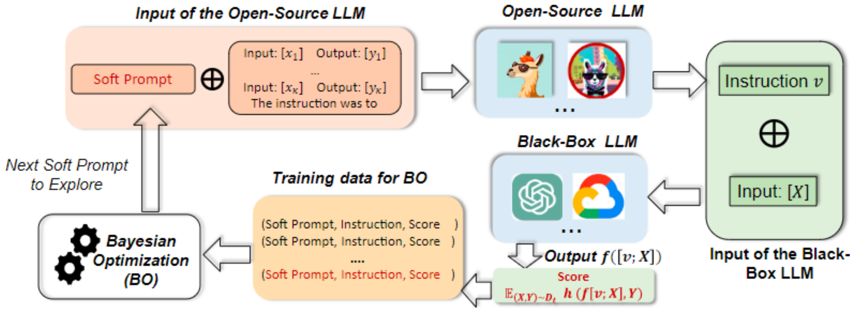
2.3. InstructZero

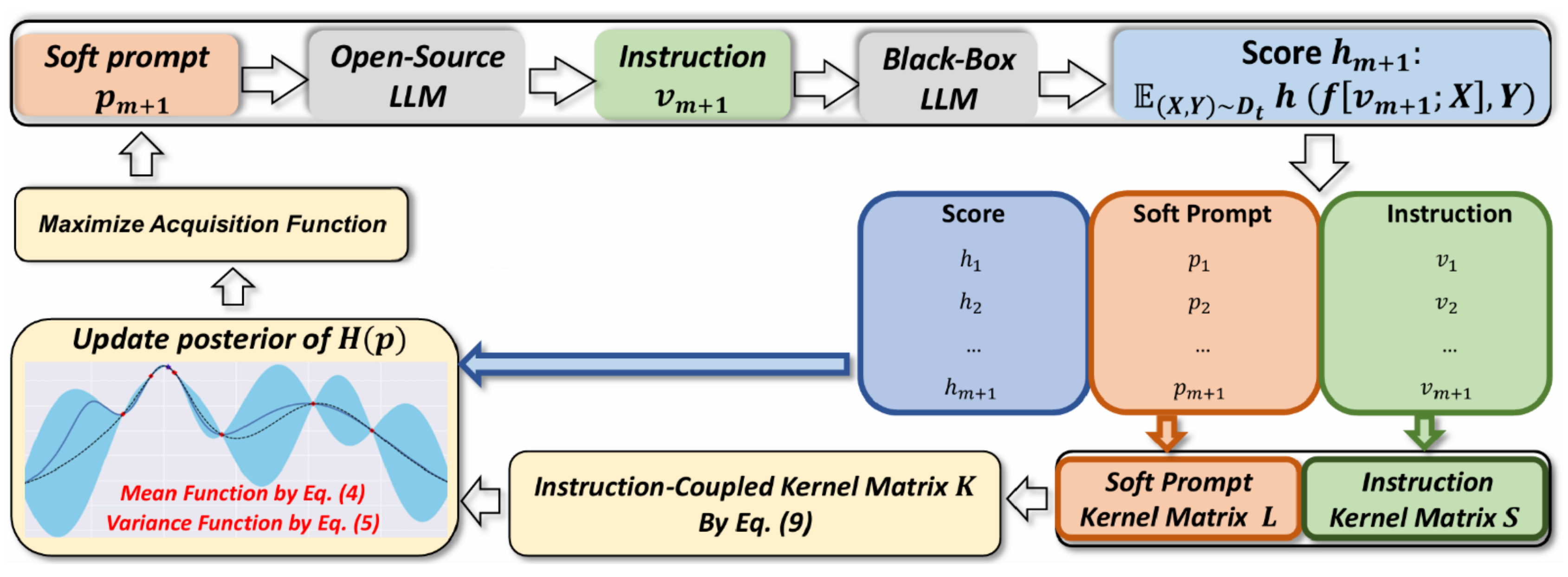
A more sophisticated approach is proposed in [14], named InstructZero. Instead of directly optimizing the prompt, which is an instruction to the LLM, InstructZero uses BO to search for the optimal prompt in a low-dimensional space associated with the embedding of an open-source LLM, which generates a human-readable and task-relevant instruction given a few examples of the target task. The instruction is then submitted to the black-box LLM. The entire pipeline is reported in Figure 3 and detailed in Figure 4.

Figure 3. Schematic representation of the iterative Bayesian optimization loop for prompt optimization in InstructZero (source: [14]).

Figure 4. Detailed pipeline of the Bayesian optimization process in InstructZero (source: [14]). The flow chart depicts the progression from soft prompts and instructions through open-source and black-box LLMs.

InstructZero uses an open-source LLM to convert a soft-prompt ($\mathbf{p}$) into an instruction that is not only task-relevant but also human-readable. The black-box LLM uses this instruction to perform zero-shot prediction, while BO estimates the relation linking every soft prompt to its associated score.

Random projection is largely used because its distance-preserving property it suitable for construct kernels. This has the important implication that the behavior of BO is consistent across the original space and the low-dimensional space. This property is particularly important for in-context learning, in that low-dimensional soft prompts can produce task-relevant instructions. The similarity between two prompts is measured in terms of correlation, usually by a Matern or a square exponential kernel. InstructZero proposes a kernel function that is task-specific:

$$s\left(v_i,v_j\right)=E_{X\sim D_t}\left[sim\left(f\left(\left[v_i;X\right]\right),f\left(\left[v_j;X\right]\right)\right)\right]$$

(5)

where $sim\left(.,.\right)$ is the similarity of the predictions for the tasks (e.g., exact match, F1, or BLEU score). Then, the two kernels are combined in an instruction-coupled kernel, which, applied to the soft prompts, recovers the instruction matrix. Then, the instruction-coupled kernel drives the combination of the two kernels and aligns BO in the latent space. The structure of the algorithm is captured in the following pseudo code (Algorithm 1).

Algorithm 1: InstructZero

Input:     Examples $\left(\overline{\mathbf{X}},\overline{\mathbf{Y}}\right)$ and a validation set $\left(\mathbf{X},\mathbf{Y}\right)$, instruction generator LLM $g(.)$, solver     LLM $f(.)$, maximal steps $T$, random projection matrix $\mathbf{A} \in {\mathbb{R}}^{d\times q}$. Initialize:     $\mathbf{P}\sim Uniform\left({\mathbb{R}}^d\right)$; $m\leftarrow 1$; $\mathbf{V}\leftarrow \varnothing$; $\mathbf{H}\leftarrow \varnothing$. while $m\le T$ do:     generate instruction ${\mathbf{v}}_m\leftarrow g\left(\mathbf{A}{\mathbf{p}}_m;\left(\overline{\mathbf{X}},\overline{\mathbf{Y}}\right)\right)$ through the open-source LLM $g(.)$     evaluate zero-shot score $h_m\leftarrow h\left(f\left({\mathbf{v}}_m,\mathbf{X}\right),\mathbf{Y}\right)$ on the black-box LLM $f\left(.\right)$     $\mathbf{P}\leftarrow \mathbf{P}\cup \left\{{\mathbf{p}}_m\right\}$     $\mathbf{V}\leftarrow \mathbf{V}\cup \left\{{\mathbf{v}}_m\right\}$     $\mathbf{H}\leftarrow \mathbf{H}\cup \left\{h_m\right\}$     update the instruction-coupled kernel matrix for P     update the posterior mean and variance function of BO     find the next prompt ${\mathbf{p}}_{m+1}$ maximizing the acquisition function (i.e., Expected     Improvement in InstructZero)     $m\leftarrow m+1$ End Output:     the best instruction ${\mathbf{v}}_{i^{\ast }}$ so far, where $i^{\ast }\in arg\underset{i\in \left[m\right]}{\max }{h}_i$

3. Bayesian Optimization for Instruction Selection (BOInG)

In this section, we detail our proposed approach, BOInG. First, we introduce some useful notations:

${\mathcal{M}}_g$: The LLM working as instruction generator. It receives a hard prompt and a small set of examples ($\left(\overline{\mathbf{X}},\overline{\mathbf{Y}}\right)\sim \mathcal{D}$) as input and produces a text representing an instruction.

${\mathcal{M}}_s$: The LLM working as solver for a certain task. It receives an instruction and a large set of input examples, that I, $\mathbf{X}$ from $\left(\mathbf{X},\mathbf{Y}\right)\sim \mathcal{D}$, as input and provides its own predictions ($\widehat{\mathbf{Y}}\approx \mathbf{Y}$).

$\mathbf{w}\in W^{\tau }$: A hard prompt consisting of $\tau$ tokens given as input to ${\mathcal{M}}_g$, with $W$, a vocabulary, preferably the one which ${\mathcal{M}}_g$ has been trained on.

$\mathcal{E}={\left\{{\mathbf{e}}_i\right\}}_{i=1}^{\left|W\right|}$: The set of the token embeddings such that ${\mathbf{e}}_i=encode\left(W_{\left[i\right]}\right)$ and $W_{\left[i\right]}=decode\left({\mathbf{e}}_i\right)$, where $W_{\left[i\right]}$ represents the $i$-th token in the vocabulary ($W$).

$\mathbf{p}\in \mathcal{P}\subset {\mathbb{R}}^d$: A soft prompt in a convenient low-dimensional search space.

We consider the same workflow as in InstructZero [14] and Instinct [15], that is, ${\mathcal{M}}_g$ works as an instruction generator; then, ${\mathcal{M}}_s$ works as a solver for a certain task by using the instruction generated by ${\mathcal{M}}_g$. The workflow starts by injecting a hard prompt ($\mathbf{w}\in W^{\tau }$) into ${\mathcal{M}}_g$, along with a small set of examples ($\left(\overline{\mathbf{X}},\overline{\mathbf{Y}}\right)\sim \mathcal{D}$). The generated instruction, denoted by ${\mathcal{M}}_g\left(\mathbf{w}⨁\left(\overline{\mathbf{X}},\overline{\mathbf{Y}}\right)\right)$, is given as input to ${\mathcal{M}}_s$, along with a large set of input examples ($\mathbf{X}$) whose associated output ($\mathbf{Y}$) must be predicted. The symbol $⨁$denotes the concatenation operator.

The final aim is to efficiently search for

$${\mathbf{w}}^{\ast }\in \underset{\mathbf{w}\in W^{\tau }}{\mathrm{argmax}}\mathcal{L}\left({\mathbf{w};\mathcal{M}}_g,{\mathcal{M}}_s,\left(\overline{\mathbf{X}},\overline{\mathbf{Y}}\right),\left(\mathbf{X},\mathbf{Y}\right)\right)$$

(6)

with the loss function defined as follows:

$$\mathcal{L}\left({\mathbf{w};\mathcal{M}}_g,{\mathcal{M}}_s,\left(\overline{\mathbf{X}},\overline{\mathbf{Y}}\right),\left(\mathbf{X},\mathbf{Y}\right)\right)={\displaystyle \frac{1}{N}}\sum _{i=1}^N{1}_{y_i}={\mathcal{M}}_s\left({\mathcal{M}}_g\left(\mathbf{w}⨁\left(\overline{\mathbf{X}},\overline{\mathbf{Y}}\right)\right)⨁{\mathbf{x}}_{\mathbf{i}}\right)$$

(7)

where $1_{a=b}$ denotes the indicator function (equal to 1 if and only if $a=b$ and 0 otherwise) and ${\mathcal{M}}_s\left({\mathcal{M}}_g\left(\mathbf{w}⨁\left(\overline{\mathbf{X}},\overline{\mathbf{Y}}\right)\right)⨁{\mathbf{x}}_{\mathbf{i}}\right)$ is the output provided by the second LLM (${\mathcal{M}}_s$), given the input (${\mathbf{x}}_i$) and the generated instruction (${\mathcal{M}}_g\left(\mathbf{w}⨁\left(\overline{\mathbf{X}},\overline{\mathbf{Y}}\right)\right)$). The entire optimization process is summarized in Figure 5.

Figure 5. Flow chart of a prompt optimization loop, starting with a hard prompt and small example set. The process involves instruction generation via closed-source LLMs (${\mathcal{M}}_g$), prompt loss calculation using the ${\mathcal{M}}_g$’s generated output with as input for the generated instruction and training set, and Bayesian optimization. This cyclical workflow illustrates the generation of instructions in the BOInG algorithm.

Solving problem (6) is difficult due to the combinatorial nature of the search space, that is, $W^{\tau }$. As already addressed in the recent literature, our idea is to, instead, use a soft prompt ($\mathbf{p}\in \mathcal{P}\subset {\mathbb{R}}^{d\times \tau }$), where $\tau$ is the number of tokens and $d$ is the dimensionality of the latent representation of each token. The most natural and suitable choice for the latent representation of the tokens should be ${\mathcal{M}}_g$’s embedding space ($\mathsf{\Omega }\in {\mathbb{R}}^q$), which, unfortunately, is usually high-dimensional, i.e., $q\gg d$. Accounting also for $\tau$, the final search space is ${\mathsf{\Omega }}^{\mathsf{\tau }}\in {\mathbb{R}}^{q\times \tau }$; on the contrary, we want to identify a conveniently low-dimensional search space ($\mathcal{P}\in {\mathbb{R}}^{d\times \tau }$) to perform BO.

As suggested in the recent literature, we use a random projection matrix ($\mathbf{A}\in {\mathbb{R}}^{d\times q}$), with entries sampled from a normal or uniform distribution to project any soft prompt ($\mathbf{p}$) from our conveniently low-dimensional search space ($\mathcal{P}$) into an associated point in the high-dimensional search space (${\mathsf{\Omega }}^{\mathsf{\tau }}$). Thus, each $d$-dimensional token (${\mathbf{p}}_{\left[i\right]}$) of the prompt ($\mathbf{p}$) is projected into an embedding ($\mathbf{A}{\mathbf{p}}_{\left[i\right]}$). Random projection is a quite common procedure known to be distance-preserving. However, the projection of the soft prompt is still not a hard prompt, which is, instead, needed as an input of the instruction generator (${\mathcal{M}}_g$).

It is important to remark that the embeddings of the tokens used to train ${\mathcal{M}}_g$ all lie within the high-dimensional space ($\mathsf{\Omega }$) and are denoted as set $\mathcal{E}={\left\{{\mathbf{e}}_i\right\}}_{i=1}^{\left|W\right|}$, where ${\mathbf{e}}_i=encode\left(W_{\left[i\right]}\right)$ and $W_{\left[i\right]}=decode\left({\mathbf{e}}_i\right)$. Thus, the most naïve strategy is to recast every projection ($\mathbf{A}{\mathbf{p}}_{\left[i\right]}$) into the closest ${\mathbf{e}}_j\in \mathcal{E}$, then retrieve the associated token ($W_{\left[j\right]}$). This allows for the retrieval of a hard prompt ($\mathbf{w}\in W^{\tau }$) given the random projection of a given soft prompt ($\mathbf{p}\in \mathcal{P}$) the computation of the associated loss. Although this is a possible procedure, we later find that it can be largely ineffective.

At a generic iteration ($n$) of BO, the trials (${\mathbf{p}}^{\left(1\right)},\dots ,{\mathbf{p}}^{\left(n\right)}$) and the associated losses (${\mathcal{L}}^{\left(1\right)},\dots ,{\mathcal{L}}^{\left(n\right)}$) are used to train a GP approximating a back-box and expensive loss function with respect to soft prompts ($\mathbf{p}$) in the low-dimensional space ($\mathcal{P}$). Selection of the next prompt to try (${\mathbf{p}}^{\left(n+1\right)}$) is performed by optimizing an acquisition function balancing between exploration and exploitation. However, due to random projection induced by $\mathbf{A}$, we are not sure that the projected point ($\mathbf{A}\mathbf{p}$) is “consistent” with the (embeddings of the) tokens known to ${\mathcal{M}}_g$. In simpler terms, in a very high-dimensional space ($\mathsf{\Omega }$), the projected point ($\mathbf{A}{\mathbf{p}}_{\left[i\right]}$) could be far away from the embedding of any token known to ${\mathcal{M}}_g$, leading the LLM to generate incomprehensible and strange instructions that are difficult for ${\mathcal{M}}_s$ to successively interpret.

Indeed, we introduce a penalty function ($\pi \left(\mathbf{p}\right)$) so that UCB is optimized while keeping all the projections ($\mathbf{A}{\mathbf{p}}_{\left[i\right]}$) associated with the soft prompt ($\mathbf{p}\in \mathcal{P}$) as close as possible to the embeddings of the tokens known to ${\mathcal{M}}_g$. Our penalty function is defined as follows:

$$\pi \left(\mathbf{p}\right)={\displaystyle \frac{1}{\tau }}\sum _{i=1}^{\tau }\underset{e\in \mathcal{E}}{\min }‖\mathbf{A}{\mathbf{p}}_{\left[i\right]}-\mathbf{e}‖$$

(8)

In more simple terms, $\pi \left(\mathbf{p}\right)$ is the average distance between each projection ($\mathbf{A}{\mathbf{p}}_{\left[1\right]},\dots ,\mathbf{A}{\mathbf{p}}_{\left[\tau \right]}$) from the closest embedded tokens known to ${\mathcal{M}}_g$. Finally, ${\mathbf{p}}^{\left(n+1\right)}$ is obtained as follows:

$${\mathbf{p}}^{\left(n+1\right)},{\mathbf{w}}^{\left(n+1\right)}\in \underset{\mathbf{p}\in \mathcal{P}}{\mathrm{argmax}}\mu \left(\mathbf{p}\right)+\beta \sigma \left(\mathbf{p}\right)-C\pi \left(\mathbf{p}\right)$$

(9)

where $C$ is a regularization hyperparameter and $\beta$ manages the exploration–exploitation trade-off. Indeed, the usual UCB is penalized by the quantity expressed as $C\pi \left(\mathbf{p}\right)$.

It is important to remark that solving the penalized UCB requires computation of $\pi \left(\mathbf{p}\right)$; thus, we obtain ${\mathbf{p}}^{\left(n+1\right)}$, along with the associated indices ($j_i^{\ast }=\underset{j=1,\dots ,\left|W\right|}{\mathrm{argmin}}‖\mathbf{A}{\mathbf{p}}_{\left[i\right]}-{\mathbf{e}}_j‖$) for each $i=1,\dots ,\tau$, from which we directly obtain the associated hard prompt (${\mathbf{w}}^{\left(n+1\right)}$) such that ${\mathbf{w}}_i^{\left(n+1\right)}=decode\left({\mathbf{e}}_{j_i^{\ast }}\right)=W_{\left[j_i^{\ast }\right]}$. This is crucial: we are searching in the conveniently low-dimensional search space ($\mathcal{P}$) but close to known embeddings, which is completely different form optimizing UCB “freely”, then recasting ${\mathbf{p}}^{\left(n+1\right)}$ to the closest embeddings a posteriori. In the second case, UCB could lead to a ${\mathbf{p}}^{\left(n+1\right)}$ so far away from all the known tokens (due to the high dimensionality of ${\mathsf{\Omega }}^{\tau }$) that recasting could be completely incoherent.

Finally, knowing the embeddings of the tokens known to ${\mathcal{M}}_g$ is the best option for the proposed approach; however, this requires ${\mathcal{M}}_g$ to be a white-box model. To mitigate this request and give the chance to, instead, use powerful black-box LLMs, we decided to only adopt the embeddings of another white-box LLM–specifically, GPT2 in our case–under the assumption that the distances between embeddings should be coherent across different LLMs.

GPT-3.5 Turbo is used in BOInG as an LLM. For each task, we use the following parameter settings: 5 and 20 samples from the training and validation sets, respectively. The number of tokens in every soft prompt is 5. The elements of the random projection matrix are sampled from a uniform distribution in $[-\mathrm{1,1}]$. The value of $d$ is set to 10, and 25 soft prompts are explored for each iteration. Finally, $\beta =1$ and $C=1$.

We utilized an evolutionary search algorithm, namely “SampleReducingMCAcquisitionFunction”, to find the top 25 soft prompts. All training and testing were performed on a 4-core machine equipped with an NVIDIA T4 GPU, which accelerated the matrix calculations necessary for determining the penalty (obtaining the embedding distances). The BOInG algorithm is summarized in the following (Algorithm 2).

Algorithm 2: BOInG (Bayesian Optimization for Instruction Generation)

Input: Examples $\left(\overline{\mathbf{X}},\overline{\mathbf{Y}}\right)$, validation set $\left(\mathbf{X},\mathbf{Y}\right)$, instruction generator LLM ${\mathcal{M}}_g$, solver LLM ${\mathcal{M}}_s$, maximal steps $T$, the dimensionality $d$ of the search space, number of tokens τ, vocabulary $W$, embeddings set $\mathcal{E} = {\left\{{\mathit{e}}_i\right\}}_{i=1}^{\left|W\right|}$, random projection matrix $\mathbf{A} \in {\mathbb{R}}^{d\times q}$. Initialize:     $\mathbf{P}\leftarrow Sobo{l}_{initialization}$ (n = 10)     $\mathbf{V}\leftarrow \varnothing$; $\mathbf{L}\leftarrow \varnothing$     for $\mathbf{p} \in \mathbf{P}$ do       for i = 1 to τ do         $j_i^{\ast }\leftarrow argmi{n}_{j=1,\dots ,\left|W\right|}\left|\left|\mathbf{A}{\mathbf{p}}_{\left[i\right]}-{\mathbf{e}}_j\right|\right|$         ${\mathbf{w}}_{\left[i\right]}\leftarrow decode\left({\mathbf{e}}_{j_i^{\ast }}\right)=W_{\left[j_i^{\ast }\right]}$         ${\mathbf{v}\leftarrow \{\mathcal{M}}_g\left({\mathbf{w}}_{\left[i\right]}\oplus \left(\overline{\mathbf{X}},\overline{\mathbf{Y}}\right)\right)\}$         $\mathbf{V} \leftarrow \mathbf{V}\cup \left\{\mathbf{v}\right\}$         $\mathbf{L} \leftarrow \mathbf{L}\cup \left\{1/N{\sum }_{i=1}^{N}1\left({\mathbf{y}}_i={\mathcal{M}}_s\left(\mathbf{v}\oplus {\mathbf{x}}_i\right)\right)\right\}$       end for     end for while $\left|\mathbf{L}\right|\le T$ do     train a GP model using ($\mathbf{P},\mathbf{L}$)     ${\mathbf{p}}^{\prime },{\mathbf{w}}^{\prime }\leftarrow \underset{\mathbf{p}\in \mathcal{P}}{\mathrm{argmax}}\left(\mu \left(\mathbf{p}\right)+\beta \sigma \left(\mathbf{p}\right)-C\pi \left(\mathbf{p}\right)\right)$//Penalized UCB     ${\mathbf{v}}^{\prime }\leftarrow {\mathcal{M}}_g\left(\left[{\mathbf{w}}^{\prime }\oplus \left(\overline{\mathbf{X}},\overline{\mathbf{Y}}\right)\right]\right)$//Generate instruction using Instruction Generator     $\mathbf{L}\leftarrow \mathbf{L}\cup \left\{1/N{\sum }_{i=1}^{N}1\left(y_i={\mathcal{M}}_s\left(v_n\oplus x_i\right)\right)\right\}$//Evaluate instruction     $\mathbf{P}\leftarrow \mathbf{P}\cup {\mathbf{p}}^{\prime }$,     $\mathbf{V}\leftarrow \mathbf{V}\cup {\mathbf{v}}^{\prime },$ end while Output:     The best instruction ${\mathbf{V}}_{\left[i^{\ast }\right]}$ with $i^{\ast }\in \underset{i=1:\left|L\right|}{\mathrm{argmax}}{\mathbf{L}}_{\left[i\right]}$ Where:     $\pi \left(\mathbf{p}\right)=1/\tau {\sum }_{i=1}^{\tau }\underset{\mathbf{e}\in \mathcal{E}}{\min }\left|\left|\mathbf{A}{\mathbf{p}}_{\left[i\right]}-\mathbf{e}\right|\right|$//Penalty function

4. Computational Results

4.1. Evaluation Metrics

Different score functions were considered depending on the specific task. In detail, we used the following four evaluation metrics:

Exact Match (EM): The correct response yields $EM=1$ and $EM=0$ otherwise. The associated tasks are “Letters list” and “Second word letter”.

Exact Set (ES): When evaluating each question-and-answer pair, $ES=1$if the predicted response precisely matches the correct responses set and $ES=0$ otherwise. The associated task is “Taxonomy”.

Contain: This measure has a value of Contain = 1 in the case that the predicted answer is part of the correct responses and Contain = 0 otherwise. The associated tasks are “Word Sorting” and “Synonyms”.

F1: The usual F1 score calculated by comparing individual words in the predicted response to those in the actual or true Answer. The common words between the predicted and actual answers form the basis for the F1 score. Precision is determined by the proportion of common words to the total words in the predicted response, while recall is calculated as the proportion of common words to the total words in the actual answer. The associated task is “Common”.

4.2. Selected Tasks

The tasks were selected from [14]; due to budgetary constraints, we selected a subset of 6 among the original 24 tasks to reduce the required testing and implementation time. The selected tasks were chosen to be representative of different levels of difficulty (based on the scores reported for APE, Uniform, and InstructZero).

Easy tasks:

Letter list: Provide the input string, separating each character with a space.

Word sorting: With a list as input, the task is to produce an output that is the list in alphabetical order.

Challenging tasks:

Taxonomy: Create a program that generates a list of animals based on the provided input.

Synonyms: Provide the synonyms of the input word.

Second word letter: Taking a string as input, return the second character.

Common: Extract the relationship between the input words.

Table 1 summarizes the results obtained by BOInG on the selected tasks and compares them against three other methods. BOInG’s test score is in line with other BO-based approaches (i.e., Instinct and InstructZero) and outperforms them on two tasks.

Table 1. Test scores comparing BOInG against APE, Instinct, and InstructZero (* for APE and Instinct results from [15]; ** for InstructZero results from [14]).

Task	Difficulty	BOInG	APE **	Instinct **	InstructZero *
Synonyms	Challenging	0.30	0.36	0.30	0.38
Common	Challenging	0.17	0.07	0.21	0.15
Letter List	Easy	1.00	1.00	1.00	1.00
Taxonomy	Challenging	0.82	0.35	0.85	0.82
Word Sorting	Easy	0.65	0.33	0.51	0.64
Second Word Letter	Challenging	0.93	0.75	0.10	0.62

An important consideration is the significantly different costs entailed by the three methods. BOInG requires the invocation of ${\mathcal{M}}_g$ via an API, implying a minimal additional cost of approximately USD 0.01 per 20′270 tokens (using GPT-3.5-turbo-0125, ANI Technologies Pvt.Ltd., Bengaluru, India). This cost is significantly lower than that required to run white-box LLMs. For instance, the GPU time required for InstructZero (using an NVIDIA A6000, NVIDIA, Santa Clara, CA, USA) would cost approximately USD 0.01 for just 25 s, during which only a few local LLM calls could be executed.

Finally, we provide some examples of generated instructions and associated hard prompts over the BO process. In Table 2, the “hard prompt” column displays the hard prompt prepended to the input given to the instruction generator LLM (${\mathcal{M}}_g$), consisting of seemingly random character strings that represent the algorithm’s exploration in the prompt space. The Instruction column shows the human-readable, task-relevant instructions generated by ${\mathcal{M}}_g$ based on these hard prompts and task examples. The “score (train)” column indicates the performance of each instruction, ranging from 0 to 1, with higher scores denoting better performance. The table captures the optimization process across six rows, including initialization and subsequent iterations. Initially, two different hard prompts yield similar instructions with identical scores of 0.40. The third iteration shows a marginal improvement, achieving a score of 0.45. The fourth row demonstrates the best performance, reaching a score of 0.55 with the instruction, “Provide synonymous terms for the given words”. This table showcases the algorithm’s progression in identifying increasingly effective instructions for the synonym task.

Table 2. The presented table illustrates the iterative process of instruction optimization for a synonyms task (no further improvement after the 3rd BO iteration).

	Hard Prompt	Instruction	Score (Train)
Best on random initialization	waalf addingolatedprom	Provide synonymous words for each input.	0.40
Best at 1st BO iteration	waalf addedolated leng	Provide alternative words for each given input.	0.40
(Two) best at 2nd BO iteration	ceryalfPOST withdrawnitia veyalf speakingvelopitia	Provide synonyms for the given words. Provide alternative words that are synonyms for the given input words.	0.45
Best at 3rd BO iteration	ceryge Sleepaos safegu	Provide synonymous terms for the given words.	0.55

5. Conclusions, Limitations, and Perspectives

BOInG demonstrates the versatility and efficiency of Bayesian Optimization (BO) for black-box problems in tackling the highly structured combinatorial challenges of prompt tuning and instruction generation in LLMs.

By leveraging an “as-a-service” API paradigm and treating both models as black boxes, BOInG avoids the need for the white-box instruction generation model’s architecture, offering greater flexibility. This approach enables BOInG to utilize high-performing, closed-source models like GPT-4o or Claude 3.5 Sonnet without requiring significant local computational resources. Unlike methods relying on open-source LLMs that necessitate dedicated hardware such as GPUs, BOInG only requires penalty loss computations using the GPT-2 embedding layer, which is orders of magnitude smaller than the LLMs used in other approaches. Experimental results confirm BOInG’s competitive performance compared to state-of-the-art methods like InstructZero and Instinct, with substantially lower resource requirements.

While effective, BOInG relies on embeddings from GPT-2 for penalty function calculations, which may introduce coherence challenges due to the mismatch between its embedding layer and that of the primary LLM. Addressing this limitation through experimentation with alternative embeddings or model-specific penalty functions could improve compatibility and performance.

Despite the successes of BO, its limitations include challenges in handling categorical variables and problems with many variables or images, where gaussian processes (GPs) tend to underperform. For such cases, Bayesian neural networks have been suggested as promising alternatives, offering the ability to flexibly represent non-stationary behavior and handle multi-output objectives. Replacing GPs with Bayesian neural networks could enhance the robustness of BOInG in these scenarios.

An entirely different perspective is to generalize the capabilities of LLMs beyond natural language tasks, generating candidate solutions for the BO process with limited data in contexts requiring generalization from few examples.