Development of a Numerical Tool for Laminate Composite Distortion Computation Through a Dual-Approach Strategy ^†

Featured Application

Composite tooling design and manufacturing. Composite laminate design optimization through advanced simulation methods.

Abstract

Unintended shape distortions, such as spring-in, spring-back, and warping, commonly occur during the curing process of laminate composites. The source of dimensional changes at the macro-scale is residual stress. The main triggers for residual stresses at this scale are anisotropic behavior and the constraint effect of individual plies and tooling constraints. Thermoelastic residual stresses are quasi-reversible, whereas non-thermoelastic residual stresses are permanent, and the underlying mechanisms contributing to them are highly intricate. The challenges associated with simulating the curing of large-scale parts to obtain reliable engineering data are significantly influenced by factors such as thermal anisotropy, polymerization shrinkage, tool–part interaction, resin flow, and compaction. A comprehensive grasp of the involved phenomena can facilitate the creation and application of numerical tools that model the curing process, providing essential information on geometry distortion that is crucial for the overall manufacturing of structural components and assemblies. To ensure that a numerical prediction tool is dependable in terms of both accuracy and precision, it is essential to have significant experimental backing throughout the entire process, from selecting the appropriate mathematical models to calibrating the calculations of distortion values.

1. Introduction

1.1. An Overeview of the Mechanisms That Generate Shape Distortions

In curing composite laminates, the parts’ final geometry does not entirely replicate the mold shape due to inherent distortions in the process. Geometrical distortion is caused by residual stresses occurring during the manufacturing process. The distortions develop into spring-in in curved parts and warpage in flat parts. Serious problems occur during rigid aerostructure assembly, requiring precision-matching design geometries. Many times, in the past but also currently, a trial-and-error approach is employed to compensate for geometrical variations. Such methods are complex, time-consuming, and costly. They can, however, be eliminated partially or even entirely if distortions are accurately predicted during the design phase.

Many examples from the aeronautics industry are available. The rear spar of the Airbus A350 XWB wing is a 27 m long CFRP laminate part for which geometrical deviations caused by distortions during the curing phase may completely ruin the part and render it unusable in the complex assembly phase. The matter of distortion is also severe for wind turbine blades, for which the manufacturing processes are designed to optimize production costs in a single step [1,2,3]. Generally, the aerospace industry requires high tolerance accuracy for parts and assemblies, which creates real engineering challenges, especially for moving parts like control surfaces—for instance, the Bell Agusta BA609 inboard flaperon is an aerodynamic control element with several complex and critical features [4].

The investigation of global distortion starts with identifying the mechanisms that generate residual stress [5]. Developing computational models requires deep knowledge of the mechanisms generating the geometrical variations. We can look at residual stress depending on its origin and thermoelastic or non-thermoelastic nature. We will deal with micro-scale and macro-scale residual stress for a cured part. Micro-scale residual stress will develop between the fibers and the polymeric matrix and is caused by (a) CTE mismatch of fibers and resin, (b) resin shrinkage in the curing process, and (c) moisture absorption. The micro-scale residual stress does not cause part distortion.

The source of significant geometry changes is the macro-scale residual stress. The individual ply behavior is anisotropic; the tooling and the individual plies influence the macro-scale residual stress. A general but entirely accurate assumption for thermoelastic residual stress is that the full-scale phenomena can be interpreted as a difference between in-plane thermal strain and orthogonal (through laminate thickness) thermal strain. On the other hand, non-thermoelastic stress develops through several distinct mechanisms. It leads to non-reversible geometry distortion: tool–part interaction [6], chemical shrinkage during polymerization [7], consolidation [8], laminate through-thickness degree of cure [9], and fiber volume fraction gradients [10]. An overview of these mechanisms and a high-level approach to developing a numerical tool for evaluating composite distortion is described in Figure 1.

Figure 1. Illustration of distortion mechanisms in laminates.

Multiple concurring factors cause residual stresses and the resulting distortion. Out-of-plane deformations of curved parts are caused by resin cure shrinkage and thermal anisotropy as through-thickness contraction occurs. Both factors influence distortion in different phases of the manufacturing process: shrinkage occurs during curing, and anisotropy influences cooling [11,12].

Tool–part interaction is an essential factor that influences distortion. The residual stress between a tool and a part is, in essence, caused by the different thermal behavior of the two elements, leading to shearing stress between them. The stress at the tool face is transmitted through the thickness to a certain point due to the slipping motion between the plies and the shear compliance of the resin [12,13]. For flat parts, such through-thickness stress gradients lead to warpage when the part and tool are separated [14]. The intrinsic nature and specificity of laminate manufacturing factors like through-thickness fiber volume fraction gradient and fiber alignment deviations (ply misalignment, fibers wrinkling, etc.) will lead to residual stresses and distortion [15].

Although environmental factors, such as moisture absorption, can cause distortion [16], the current study will only focus on distortions induced by thermal changes and phase changes in polymer matrices.

1.2. The Context

This article’s technological and scientific developments are credited to the project ELADINE—Evaluation of Laminate Composite Distortion by an Integrated Numerical-Experimental Approach [17]. The project was a supporting activity (CfP) for the OPTICOMS project [18] developed under the Clean Sky 2 European Program and financed by the European Commission. ELADINE aimed to create an innovative numerical tool for the spring-in prediction of primary structural components of a passenger commuter aircraft wing through an approach in which the numerical simulation development and validation were based on experimental curing data. This numerical and experimental work started on simple flat coupons and was further scaled to C-shaped coupons, a small-scale wing section demonstrator, and a full-size 7 m wing demonstrator.

1.3. The Existing Numerical Tools and Simulation Capabilities

Given the context, the research work needed first to establish which simulation tools represent the industry standard for predicting composite distortion. One of the most-cited software packages is ESI PAM DISTORTION [19], along with a more comprehensive software package frame simulation module called PAM COMPOSITES. As claimed on the ESI web page, the simulation tool allows the prediction of manufacturing-induced residual stresses and shape distortion of composite parts made of continuous fibers and thermoset matrices. One of the newer simulation solutions, credited with a similar approach and similar capabilities to PAM DISTORTION, is ALTAIR Advanced Cure Simulation [20], which promises to allow users to predict polymerization, residual stress buildup, and deformations during composite processing.

However, it was unclear to what extent both the ESI and ALTAIR tools would allow for the tuning of curing parameters and which mechanisms causing distortion significantly influence the computed results derived according to their respective simulation strategies.

We explored the specific capabilities of other simulation environments: ANSYS PrepPost [21], ABAQUS/Standard [22], COMSOL Multiphysics Nonlinear Structural Materials Module [23], and MSC Marc Advanced Nonlinear Simulation Solution [24]. Each simulation environment offers the means for developing a custom numerical tool for predicting composite distortion. The choice was made to use the MARC simulation solution due to our previous expertise with this product and the existence of a complete element library, material models, and robust non-linear algorithms. We previously used MARC to simulate large deformations, general contact, and coupled problems.

Although several simulation environments can be chosen, the ESI and ALTAIR tools were the only dedicated numerical tools for simulating thermoset distortion.

The ELADINE work supported the development of a specific airframe part for which distortions needed to be evaluated and compensated through the geometry design of the tools. The authors accept that the exploratory work was carried out for a particular scope, but the ambition and potential of a numerical tool capable of predicting distortion goes far beyond a unique part. A numerical tool can consistently simulate the general behavior of thermoset resins and apply them to most distortion analysis scenarios under the condition that a thorough assessment of the curing parameters of the employed materials is achieved. Severe challenges for predicting distortion are met when scaling simulations from small coupons to full-scale parts.

One important factor to mention is that the methods and tools described in the article only apply to thermoset resins and not to thermoplastics. The article does not account for thermoplastics, although several methods, primarily experimental investigations, also apply to this particular class of polymers.

2. The Numerical Tool Development

2.1. The Development of the Simulation Strategy

2.1.1. Thermal Anisotropy

The coefficient of thermal expansion (CTE) is more significant in resins than fibers. This mismatch results in a phenomenon called thermal anisotropy, which can be defined as a higher contraction or expansion in the resin-dominant direction than in the fiber-dominant direction.

Distortions of this nature do not occur in flat plates; rather, they manifest in curved geometries. This is due to the difference in the coefficient of thermal expansion (CTE) between the thickness direction and the circumferential direction, which decreases the enclosed angle in curved areas—a phenomenon referred to as spring-in. Such effects do not apply to isotropic materials, where contraction and expansion are consistent. In fiber-reinforced composites, the CTE and strains in the through-thickness direction are significantly greater than those in the fiber direction, leading to a reduction in the enclosed angle ($\theta$), as generically illustrated in Figure 2.

Figure 2. A reduction in enclosed angle due to contraction results in the spring-in deformation pattern.

The first attempt to calculate the magnitude of the enclosed angle was proposed by Nelson and Cairns [25] with the following:

$$\mathrm{\Delta }\theta =\theta {\displaystyle \frac{({\alpha }_{\theta }-{\alpha }_R)\mathrm{\Delta }T}{1+{\alpha }_R\mathrm{\Delta }T}}$$

(1)

where

• $\mathrm{\Delta }\theta$ is the spring-in angle;
• $\theta$ is the subtended angle of the part;
• ${\alpha }_{\theta }$ is the circumferential coefficient of thermal expansion;
• ${\alpha }_R$ is the radial coefficient of thermal expansion;
• $\mathrm{\Delta }T$ is the temperature change.

2.1.2. Polymerization Shrinkage

During the polymerization of thermosets, the liquid resin transforms into a rigid, brittle solid through a chemical cross-linking process, resulting in an increased density and a reduced volume. The resin experiences shrinkage primarily during the curing phase. The extent of composite shrinkage differs between the in-plane directions and the through-thickness direction, influenced by the constraints imposed by the fibers. Consequently, shrinkage strains are more pronounced in the transverse direction than in the fiber direction.

To account for the impact of cure shrinkage on spring-in, Radford and Diefendorf [26] incorporated a cure shrinkage term, leading to the expression of the spring-in angle:

$$\mathrm{\Delta }\theta =\theta \left[{\displaystyle \frac{({\alpha }_{\theta }-{\alpha }_R)\mathrm{\Delta }T}{1+{\alpha }_R\mathrm{\Delta }T}}+{\displaystyle \frac{{\epsilon }_{\theta }-{\epsilon }_R}{1+{\epsilon }_R}}\right]$$

(2)

where

• ${\epsilon }_{\theta }$ is the in-plane chemical shrinkage strain;
• ${\epsilon }_R$ is the through-thickness chemical strain.

2.1.3. Tool–Part Interaction

In the curing process, the mold and the composite component are pressed together under a specific pressure while undergoing a temperature increase. This leads to a shear interaction at the interface due to the differing coefficients of thermal expansion (CTEs) of the two materials. Notably, areas of the composite that do not engage with the tool do not experience this shear interaction. Consequently, a non-uniform stress distribution is established, which becomes permanent as the resin hardens. Upon detaching the composite part from the tooling, these stresses induce bending moments, resulting in shape distortions, including warpage in the composite components, as is graphically described in Figure 3.

Figure 3. Effect of tool–part interaction on distortion: (a) flat parts; (b) parts that have corner sections.

2.1.4. Resin Flow and Compaction

Resin flow is crucial in determining the fiber volume fraction distribution, influencing the laminate’s mechanical properties and the component’s final dimensions [27]. Due to the non-uniform nature of resin injection, areas with varying resin concentrations—both resin-rich and resin-poor—can develop. A bleeder can be utilized within the vacuum bag during laminate manufacturing to achieve a more consistent resin distribution. This approach enables liquid resins to migrate and bleed through the thickness of the laminate. Flat laminates are most prone to warpage and distortion, as shown in Figure 4. Thin-walled structures with no stiffeners are susceptible to warping.

Figure 4. Effect of resin flow on the warpage in flat laminates.

In the case of curved components, the phenomenon that leads to a non-uniform distribution of fiber content in the through-thickness direction is referred to as fiber bridging. During the compaction process, as the thickness of the component diminishes, the friction between the prepreg layers inhibits their ability to adapt to the tool’s shape, particularly at the corners. Consequently, the pressure applied is ineffective at these corners due to fiber bridging. This results in the formation of a low-pressure zone at the tool’s corner, which is subsequently infiltrated by resin, thereby increasing the thickness of the component in that area and creating a region rich in resin, as illustrated in Figure 5.

Figure 5. Corner thickening due to resin flow from arms to corners.

2.1.5. Temperature Gradients

The phenomenon of transient heat transfer induces thermal gradients that lead to variations in polymerization, shrinkage, and the development of the modulus of the matrix material in the through-thickness direction, ultimately producing residual stresses. In thin components, the through-thickness temperature gradients are minimal and can often be disregarded; however, in thicker components, the rapid generation of heat combined with the lower thermal conductivity of the composite can create substantial temperature and curing gradients [28].

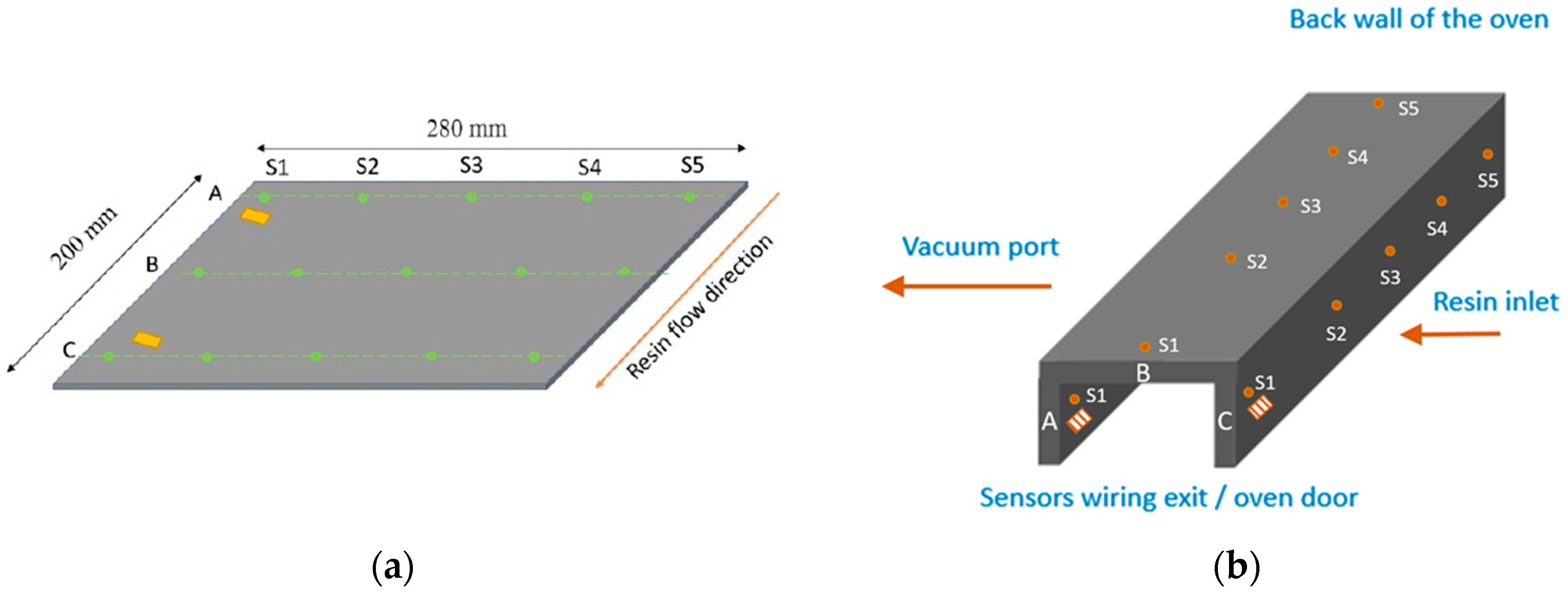
2.1.6. The Experimental Approach to Manufacturing Process Monitoring

Monitoring critical process parameters is the most dependable method for comprehending the extent of distortion mechanisms, particularly during the manufacturing phases. An experimental program was conducted using composite coupons. Figure 6 is a graphic description of the experimental program strategy for obtaining the much-needed curing process data.

Figure 6. Illustration of the overall aim of the experimental program.

The manufacturing process was meticulously observed through the integration of fiber Bragg grating (FBG) optical sensors and dielectric sensors (DCs). The data collected from this monitoring were utilized to calibrate a finite element method (FEM) simulation tool aimed at predicting shape distortion in large integral composite wing structures [29]. The experimental program utilized FB sensors to assess temperature and strain in the coupons and test specimens, while DC sensors were employed to evaluate the degree of resin curing [29].

Figure 7 illustrates the spatial arrangement of the sensors on each coupon geometry. The FBG sensors were organized into three arrays (labeled A, B, and C), each comprising five sensors (designated S1 through S5). An identical configuration was applied to both sides of the laminate: the surface in contact with the tool (lower side) and the surface interacting with the infusion consumables (upper side). No sensors were installed between the layers to prevent damage to the previously consolidated laminate. Furthermore, two DC sensors were strategically placed adjacent to the resin inlet and the vent to facilitate in-plane impregnation monitoring. Composite tools were shaped and manufactured to minimize part–tool interaction during the cooling phase. Ultimately, the shape distortions of the manufactured coupons were assessed using a 3D coordinate measurement machine (CMM) alongside FBG sensors to monitor residual stresses [29].

Figure 7. (a) Sensor distribution on skin coupons: FBG sensors (green dots) and DC sensors (squares). (b) Sensor distribution on C-spar coupons: FBG sensors (orange dots) and DC sensors (squares) [21].

The observation of variations in the Bragg wavelength allows for the assessment of multiple parameters. Changes in strain and temperature will alter the characteristics of the grating, resulting in a shift in wavelength. To distinctly identify the impact of each parameter, two distinct fiber Bragg grating (FBG) sensors were employed, one exhibiting a different thermal sensitivity. The RTM6 and RTM6-2 time–temperature resin curing cycle is described in Figure 8, along with the evolution of the DC sensors’ readings.

Figure 8. Epoxy resin RMT6 typical cycle monitoring results. DC disposable sensors can measure different events occurring during resin curing.

2.2. Mathematical Models: Development of the Numerical Model’s Logic

The development of a numerical model to predict complex distortions relied on established commercial simulation software, specifically MSC PATRAN, MSC NASTRAN, and MSC MARC. To conduct a numerical analysis of distortion in composite material manufacturing, a series of stages were outlined as an initial strategy to evaluate the operational capabilities of a generic model:

• Developing the geometric configuration for both the test specimen and the manufacturing tool;
• Specifying the thermal and structural material characteristics pertinent to both the specimen and the tool;
• Establishing the universal unit system to be employed throughout the simulation; constructing the finite element model (FEM), including the mesh and stacking sequence for both the coupon and the tool;
• Determining the FEM material properties for each layer, encompassing both thermal and structural attributes;
• Outlining the input parameters necessary for conducting a thermal finite element analysis, which include the initial temperature of the coupon/tool assembly, temperature fluctuations within the oven, convection effects on the outer surface of the assembly, thermal interactions between the coupon and the tool, and specific requirements for the mathematical model utilized in the finite element analysis solver to facilitate the curing calculations;
• Refining the thermal model by data obtained from experimental monitoring and, finally, developing and resolving a coupled thermal–structural finite element model that integrates structural properties such as Young’s Modulus, curing shrinkage, and viscosity with respect to temperature and cure rate.

2.2.1. Cure Kinetics

Initial numerical and experimental investigations conducted on small-scale coupons and specimens highlighted the importance of correlating numerical simulations with an appropriate cure kinetics model. Various methodologies exist for characterizing the cure kinetics of resin materials, including embedded cure kinetics models, tabular definitions, and user subroutines. In the context of curing analysis, the cure rate is determined at each time increment, with the assumption that the cure rate is a function of both the degree of cure and the temperature:

$${\displaystyle \frac{d\alpha }{dt}}=f(\alpha ,T)$$

(3)

The integration of the degree of cure is performed using the backward Euler method:

$${\alpha }_n^i=\mathrm{\Delta }t\cdot f({\alpha }_n^{i-1},T)+{\alpha }_{n-1}$$

(4)

where $i$ is the iteration number for the cure, $n$ is the current increment number, $n-1$ is the previous increment number, $f$ is a function defined by the cure kinetics model, and $\mathrm{\Delta }t$ is the increment’s time step size. In MSC MARC, the cure kinetics defines the cure rate as a function of the degree of cure and the temperature of resin materials. Different approaches are used to determine the cure kinetics of resin materials: embedded cure kinetics models, table definitions, and user subroutines.

The four cure kinetics models implemented in Marc are as follows:

• Cure kinetics model 1: by Lee, Loos, and Springer (1982);
• Cure kinetics model 2: by Scott (1991);
• Cure kinetics model 3: by Lee, Chiu, and Lin (1992);
• Cure kinetics model 4: by Johnston and Hubert (1996).

The Johnston–Hubert model was selected for the present modeling and simulation strategy due to its specific advantages:

• This model represents one of the latest advancements in the field;
• It incorporates a sophisticated array of parameters in its design;
• The accompanying documentation for this mathematical model is publicly available and readily accessible. Within this documentation, the authors have included empirical data derived from experiments conducted on materials analogous to those utilized in the ELADINE project;
• According to the findings presented in the article [30], there is a strong correlation between the experimental results and the data generated by the model, as illustrated in Figure 9.
  

  Figure 9. Comparison between (a) the numerically simulated degree of cure and (b) the Johnston–Hubert results.

Among the four cure kinetics models available in MARC, we selected the Johnston and Hubert model for our analysis [30]. To evaluate the preferred model for our simulation, we compared the degree of cure plots with the results published by Johnston and Hubert. The resulting graphs exhibit a striking resemblance and are presented in Figure 9.

The mathematical formulation proposed by Johnston and Hubert is expressed through the subsequent equations:

$${\displaystyle \frac{d\alpha }{dt}}={\displaystyle \frac{K{\alpha }^m{(1-\alpha )}^n}{1+e^{C\left\{\alpha -\left({\alpha }_{C0}+{\alpha }_{CT}T\right)\right\}}}}$$

(5)

$$K_i=A_i{e}^{-\mathrm{\Delta }{E}_i/(RT)}$$

(6)

The $A,\mathrm{\Delta }E,m,n,C,{\alpha }_{C0},{\alpha }_{CT},H_R$ parameters are explained in Table 1.

Table 1. Parameters used in the embedded resin cure kinetics model.

Variable	Description	Units
$\alpha$	Resin degree of cure	-
$T$	Resin temperature	K or R
$H_R$	Total resin heat of reaction	J/kg or BTU/lb
$A_i$	Pre-exponential factor	/s
$\mathrm{\Delta }{E}_i$	Activation energy	J/mol or BTU/mol
$m$	Equation superscript	-
$n$	Equation superscript	-
$C$	Diffusion constant	-
${\alpha }_{C0}$	Critical resin degree of cure	-
${\alpha }_{CT}$	The increase in critical resin degree of cure with temperature	-

In Table 2 are given the parameters used for HEXCEL 8552 8552 epoxy resin cure kinetics model [22].

Table 2. Parameters used for HEXCEL 8552 epoxy resin cure kinetics model [22].

Parameter	Value	Comments
Activation energy	$\mathrm{\Delta }E=66.5\mathrm{k}\mathrm{J}/\mathrm{g}\mathrm{m}\mathrm{o}\mathrm{l}\mathrm{e}$	Calculated from the slope of $\ln (d\alpha /dt)$ vs. $1/T$
Pre-exponential cure rate coefficient	$A=1.53\times {10}^5{\mathrm{s}}^{-1}$	Calculated from weighted least-squares analysis
First exponential constant	$m=0.813$	Calculated from weighted least-squares analysis
Second exponential constant	$n=2.74$	Calculated from weighted least-squares analysis
Diffusion constant	$C=43.1$	Accounts for the rate of shift from kinetics to diffusion control
The critical degree of cure at T = 0 K	${\alpha }_{C0}=-1.684$	Note that this parameter is invalid below 35 °C, since the degree of cure cannot be negative
Constant accounting for the increase in critical resin degree of cure with temperature	${\alpha }_{CT}=5.475\times {10}^{-3}{\mathrm{K}}^{-1}$	When $\alpha$ approaches ${\alpha }_C$ at a given temperature, the cure rate slows dramatically as the reaction becomes diffusion-controlled

The complete data of the specific resin system used in the experimental program and the numerical simulations are readily available in the literature.

In Figure 10, the calculated slope plot results for the values of $\alpha =0.20$, $\alpha =0.25$, and $\alpha =0.30$ are identical to the slope of the published results of Johnston–Hubert [30].

Figure 10. Graphical comparison of (a) equation linearization results in the case of the numerical simulation and (b) Johnston–Hubert results.

2.2.2. The Cure Shrinkage of the Resin

The MARC FEM tool relies on two powerful mathematical models to deal with complex simulations of materials’ behavior:

• Boghetti and Gillespie [31]. The dependence between the cure shrinkage and the degree of cure is represented as a second-order polynomial:

$$V_r^S=0.0; \alpha <{\alpha }_{C1}$$

(7)

$$V_r^S=A\cdot {\alpha }_s+\left(V_r^{S_{\infty }}-A\right)\cdot {\alpha }_S^2; {\alpha }_{C1}\le \alpha <{\alpha }_{C2}$$

(8)

$$V_r^S=V_r^{S_{\infty }}; \alpha \ge {\alpha }_{C2}$$

(9)

$${\alpha }_s={\displaystyle \frac{\alpha -{\alpha }_{C1}}{{\alpha }_{C2}-{\alpha }_{C1}}}$$

(10)

The $V_r^{S_{\infty }},{\alpha }_{C1},{\alpha }_{C2},A$ parameters are explained in Table 3.

Table 3. Parameters used in the resin cure shrinkage model.

Variable	Description	Units
$V_r^S$	Resin volumetric cure shrinkage	-
$V_r^{S_{\infty }}$	Total volumetric resin shrinkage from 0 to 1	-
${\alpha }_s$	Degree of cure shrinkage	-
${\alpha }_{C1}$	Degree of cure after which the resin shrinkage begins	-
${\alpha }_{C2}$	Degree of cure after which the resin shrinkage stops	-
A	Polynomial cure shrinkage coefficient (Bogetti and Gillespie)	-
B	Exponential cure shrinkage coefficient (White and Hahn)

2.

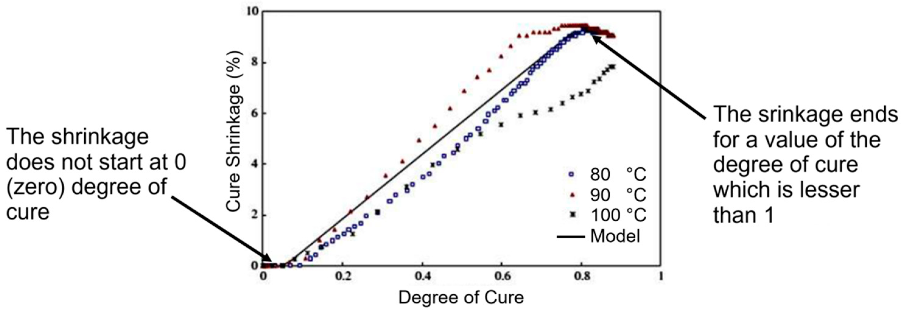
White and Hahn [32]. The curing shrinkage as a function of the degree of cure is represented as an exponential dependence:

$$V_r^S=V_r^{S\infty }\ast {10}^{B(\alpha -{\alpha }_C)}; \alpha \le {\alpha }_C$$

(11)

$$V_r^S=V_r^{S\infty }; \alpha >{\alpha }_C$$

(12)

The equations have similar parameters: $V_r^S;{\alpha }_C;B$. The cure shrinkage strain is calculated according to the volumetric shrinkage due to the curing process. The resin degree of cure shrinkage is defined as the ratio of the volumetric cure shrinkage $(V_r^s)$ and the maximum volumetric cure shrinkage $(V_r^{S_{\infty }})$ of the resin material as follows:

$${\alpha }_s={\displaystyle \frac{V_r^S}{V_r^{S_{\infty }}}}$$

(13)

Considering Bogetti and Gillespie’s mathematical formulation of cure shrinkage and the known values from Table 4, the resin cure behavior can be plotted over the entire cure cycle, as presented in Figure 11.

Table 4. Starting values for the Bogetti–Gillespie cure shrinkage model.

Parameter	Units	Value
${\alpha }_{C1}$	-	0
${\alpha }_{C2}$	-	1
$V_r^{S_{\infty }}$	-	0.02 (from Bogetti and Gillespie’s experimental results)
A	-	0.001
		0.02
		0.04

Figure 11. Variations in resin volumetric shrinkage with cure based on the Bogeti–Gillespie equation.

As defined by [31], the equations that describe the model are as follows:

$$V_r^S=0.0 when \alpha <{\alpha }_{C1};$$

(14)

and

$$V_r^S=V_r^{S\infty } when \alpha <{\alpha }_{C2};$$

(15)

$$V_r^S=A\cdot {\alpha }_S+(V_r^{S\infty }-A) when {\alpha }_{C1}\le \alpha \le {\alpha }_{C2};$$

(16)

with

$${\alpha }_S=\frac{\alpha -{\alpha }_{C1}}{{\alpha }_{C2}-{\alpha }_{C1}}$$

(17)

In the simulation, the following values were considered: ${\alpha }_{C1}=0$ and ${\alpha }_{C2}=1$—see Table 3 and Table 4. In the Bogetti–Gillespie model implemented in MARC, the “A” parameter was defined to tune the resin shrinkage versus the degree of cure dependence over the experimental data. Our calculations show that it is possible to define a linear dependence as A = 0.02, a concave dependence as A = 0.001, or a convex dependence as A = 0.04. Based on [31], we considered that the dependence between the cure shrinkage and the degree of cure is concave, as presented in Figure 12.

Figure 12. The shape of variations in resin volumetric shrinkage with cure [31].

The Boghetti–Gillespie model recommends a more conservative value of 2% less than the experiments in Figure 13, which presents the effect of variation in parameter A. In our simulation, we considered A = 0.04, corresponding to a concave dependence shape.

Figure 13. Cure shrinkage as a function of the degree of cure for a parallel plate geometry [32].

The Boghetti–Gillespie model also offers the possibility of using the $\alpha c1$ and $\alpha c2$ parameters to insert a delay phase at the start and the end of the shrinking process. This is especially important for the calibration phase of the model, as two important observations indicate:

• The shrinkage does not start at a degree of cure equal to 0, but later in the polymerization process, at a higher parameter value;
• The shrinkage does not end at a degree of cure equal to 1, but earlier in the process for a smaller parameter value.

The data presented in Figure 13 and based on the experiments from [32] confirm this assumption.

In the White–Hahn model implemented in Marc, the “B” parameter was defined to tune the resin shrinkage, like the “A” parameter in the Bogetti–Gillespie implementation. Applying values presented in Table 5, the variations in resin volumetric shrinkage vs. cure degree based on the White–Hahn equation are shown in Figure 14.

Table 5. Starting values for the White–Hahn cure shrinkage model.

Parameter	Units	Value
${\alpha }_C$	-	1
$V_r^{S\infty }$	-	0.02 (the same value as above)
$B$	-	1
		2
		4

Figure 14. Variations in resin volumetric shrinkage with cure based on the White–Hahn equation.

In the Bogetti–Gillespie model implemented in MARC, the “A” parameter was defined to tune the resin shrinkage versus the degree of cure dependence over the experimental data. Our calculations show that it is possible to define a linear dependence as A = 0.02, a concave dependence as A = 0.001, or a convex dependence as A = 0.04.

Based on reference [31], we considered that the dependence between the cure shrinkage and the degree of cure is concave, as shown in the blue plot in Figure 14.

In the White–Hahn model implemented in MARC, the “B” parameter tunes the resin shrinkage, like the “A” parameter in the Bogetti–Gillespie implementation. Figure 15 plots the variations in resin volumetric shrinkage vs. cure degree based on the White–Hahn equation.

Figure 15. A graphical comparison between the numerically simulated degree of cure and the Johnston–Hubert results.

Based on these data, we decided to use the Bogetti–Gillespie mathematical model for the following reasons:

• The model mentioned above can simulate concave and convex shapes of the variation between shrinkage and degree of cure. Based on experimental data, changing the theoretical “A” parameter to tune the model is easy. We chose a value that corresponds to a convex variation;
• The Bogetti–Gillespie model is more complex than the White–Hahn model because, by using the α_c1 and α_c2 parameters, it is possible to obtain a mathematical model closer to an actual experiment;
• Finally, the Bogetti–Gillespie model can be tuned closer to experimental trials for calibration.

2.2.3. The Resin Modulus Variation over the Curing Process

The Young’s Modulus values were known for the fully uncured resin, corresponding to the zero degree of cure value. To establish the evolution of the resin’s Young’s Modulus during the curing process, a study by Bogetti and Gillespie [23] was used. For the fully cured resin, which corresponded to a degree of cure equal to 1, the values in the (0, 1) interval were calculated using Bogetti and Gillespie’s law of variation [23]. In Bogetti and Gillespie’s research, the following formula was used:

$$E_m=(1-\alpha )E_m^0+\alpha E_m^{\infty }+\gamma \alpha (1-\alpha )(E_m^{\infty }-E_m^0)$$

(18)

where

• $E_m^0$ is the resin modulus in the fully uncured state;
• $E_m^{\infty }$ is the resin modulus in the fully cured state;
• $\alpha$ is the degree of cure;
• $\gamma$ quantifies the competing mechanisms of stress relaxation and chemical hardening, $\gamma \in \left(-1;1\right)$. Increasing $\gamma$ physically corresponds to a more rapid increase in modulus at a lower degree of cure before asymptomatically approaching the fully cured modulus.

In the case of Bogetti and Gillespie, the following resin characteristics were determined, as shown in Table 6, where the Young’s modulus are given for Epoxy resin.

Table 6. Epoxy resin’s Young’s Modulus in fully uncured and fully cured state.

Property	Units	Epoxy
$E_m^0$	MPa	3.447
$E_m^{\infty }$	MPa	3447

Because the Young’s Modulus values were known for the fully uncured resin, which corresponded to zero degrees of cure, and for the fully cured resin, which corresponded to a degree of cure of 1, the rest of the values were extracted using Bogetti and Gillespie’s law of variation.

2.2.4. The Laminate Mechanical Properties over the Curing Process

As the resin was curing, we evaluated laminate mechanical properties using the homogenization technique for the Young’s Modulus variable—described in the Figure 16 plot. The incremental step was chosen to be 5% of the cure degree, and the only evolving parameter was the corresponding resin modulus. For increased efficiency, we employed the DIGIMAT material modeling platform.

Figure 16. Variation in the Young’s Modulus of the resin with the degree of cure.

As shown in Figure 17, to calculate the properties of the composite at various degrees of cure, properties of the Young’s Modulus had to be introduced together with the Poisson’s Ratio. In the case presented above, the Young’s Modulus of the resin corresponded to a 10% degree of cure. The modulus of the resin had to be modified for each iteration of the curing process in the case of the resin, while the volumetric fraction of fibers remained constant. The software tool used for this calculation was DIGIMAT. DIGIMAT is a state-of-the-art multiscale material modeling platform focusing on the micro-mechanical modeling of complex multiphase materials such as plastics, composites, metals, and elastomers, revealing how they perform at part and system levels [33,34].

Figure 17. EPOXY resin property variation computation with DIGIMAT.

2.3. Simulation Model Structure

A Marc model was built as a thermal–structural model. The model included the following:

• A transient thermal component;
• A structural quasi-static component.

The transient thermal component handles thermal elements such as temperature variation, specific heat, thermal conduction, and thermal convection.

The structural quasi-static component handles structural components such as Young’s Modulus, Shear Modulus, Poisson’s Ratio, deformations, internal stresses, etc.

Both components run together, and each iteration solves thermal and structural components. A key parameter is needed to connect the two model components. This key parameter is α = the cure degree.

The curing degree is computed in the thermal component based on Johnston and Hubert’s implementation as a time and temperature function and specific material data. In the structural component, the curing degree is the parameter that imposes the variation in the structural parameter mentioned above. Also, based on the Bogetti and Gillespie mathematical model, the structure’s shrinkage is defined.

To illustrate the workflow logic and the functional steps of the model, we defined a model architecture diagram presented in Figure 18. It can be observed in the model functional diagram that the central component in the numerical model structure is the degree of cure space field as a function of time. To replicate the real-world scenario, the material’s mechanical properties depend on the resin’s degree of cure. The data flow used to obtain this dependency is described in the steps below:

Figure 18. Model architecture diagram.

• For each value of the degree of cure between 0 and 1, the resin has specific values of mechanical properties;
• The resin-impregnated fibers have mechanical properties that may be considered constant in the working temperature range;
• Using the DIGIMAT 2019.1 software tool and applying the homogenization theory, equivalent orthotropic material properties were computed for a resin-impregnated ply at different degrees of cure.

Before the heat transfer analysis passes, the curing analysis was performed based on the estimated temperatures at the beginning and the end of the increment. The cure rate was then calculated according to the cure kinetics of the resin materials. Using the cure rate, the heat flux due to cure reaction heat generation was calculated and added to the heat transfer system of equations. Volumetric curing reaction heat flux was calculated according to the cure rate [33]:

$$Q^C={\displaystyle \frac{d\alpha }{dt}}(1-V_f){\rho }_r{H}_r$$

(19)

where $H_r$ is the resin cure reaction, ${\rho }_r$ is the resin density, $\alpha$ is the cure degree, and $V_f$ is the fiber volume fraction.

The governing matrix equation for the cure–thermal coupled analysis is expressed as follows [33]:

$$C(T)T^{\prime }+K(T)T=Q+Q^I+Q^F+Q^C$$

(20)

In Equation (20), C(T) and K(T) are the temperature-dependent heat capacity and thermal conductivity matrices, respectively; T is the nodal temperature vector; T’ is the time derivative of the temperature vector; Q is the external heat flux vector; Q^I is the heat flux vector due to plastic work; Q^F represents the heat generated due to friction; and Q^C is the heat generated due to curing. Figure 19 is a plot illustrating the FE model’s thermal boundary conditions.

Figure 19. (a) Modeling convection at the surface of the coupon–mold assembly. (b) Modeling thermal contact between coupon and mold.

2.4. Test Cases

Two types of coupons were defined for both the experimental program and the simulation works—the coupon geometries are described in Figure 20 and Figure 21. The skin coupons were chosen with a geometry relevant to the skin from the skin–spar assembly designed by the OPTICOMS EU project [18], for which the ELADINE CfP [17] prepared the tool compensation strategy and numerical tool.

Figure 20. Illustration of the skin coupon test case—3 mm thickness.

Figure 21. Illustration of the C-coupon coupon test case.

A mildly curved panel was proposed with three distinct thickness values to cover ranges of the wing test specimen: 3.0, 6.5, and 11.5 mm. The shape of the coupon, before preforming [35,36], was a flat rectangle of 280 × 200 mm². The inner curvature radius was kept constant at 1475 mm for all three thickness coupons. The stacking sequences of the coupons were kept identical to the corresponding thickness of the skins of the OPTICOMS-designed test wing.

A geometry like the one from the C-shaped spars from OPTICOMS was selected for the more complex spar coupons. A few versions of these coupons were explored, and the final choice was two different radii flanges, as described in Figure 21. This decision was made to study the influence of corner radii on the distortion phenomena.

In Table 7 and Table 8 are illustrated the summary of ply numbers and thickness for skin coupons and C-coupons. The monitoring and simulation processes were carried out for the same coupon geometry and the same number of coupons for two distinct material systems and associated manufacturing processes: the TORAY prepreg unidirectional fiber and the HEXCEL liquid resin infusion (LRI) manufacturing processes. Table 9 presents the material systems used for coupon manufacturing and modeling.

Table 7. Skin coupons—summary of ply number and thickness.

Coupon Reference	Thickness (mm)	No. of Plies	Tests and Monitored Parameters	No. of Tests Performed
Skin1	2.5	18	Temperature and cure degree	7
			Strain and 3D CMM	3
			Manufacturing without sensors	1
Skin2	6.5	44	Temperature and cure degree	2
			Strain and 3D CMM	2
			Manufacturing without sensors	1
Skin3	11.5	80	Temperature and cure degree	2
			Strain and 3D CMM	2
			Manufacturing without sensors	1
			TOTAL	21

Table 8. C-coupons—summary of ply number and thickness.

Coupon Reference	Thickness (mm)	No. of Plies	Tests and Monitored Parameters	No. of Tests Performed
C-spar0	2.5	18	Process adjustment	6
C-spar1	3	22	Temperature and cure degree	1
			Strain and 3D CMM	1
			Manufacturing without sensors	1
C-spar2	5	34	Temperature and cure degree	2
			Strain and 3D CMM	1
			Manufacturing without sensors	1
C-spar3	3/5	22/34	Temperature and cure degree	1
			Strain and 3D CMM	1
			Manufacturing without sensors	1
			TOTAL	16

Table 9. Material systems used for coupon manufacturing and modeling.

Manufacturer	Material Description	Oven Cure Cycle
Toray	Prepreg P707AG-15, unidirectional tape T700 12K fiber and 2510 resin system. The FAW is 150 gsm (grams per square meter)	1. Dwell at 40 °C 2. Heat to 80 °C at 1 °C/minute 3. Dwell 5 Hr at 80 °C 4. Heat to 132 °C at 1 °C/minute 5. Dwell 2 Hr at 132 °C 6. Cool to RT (min. temperature 50 °C)
Hexcel	Dry fiber Hi tape unidirectional type AS7 areal weight 126 gsm RTM 6-2 resin	1. Heat tool to 120 °C, resin to 80 °C 2. Infusion process at 120 °C/80 °C 3. Heat to 185 °C at 2 °C/minute 4. Dwell 2 Hr at 185 °C 5. Cool to RT (min. temperature 50 °C)

3. Results

During the initial development phase, numerical trials were performed for small-scale coupons with geometries identical to those of the experimental trials. The low-curvature skins and C-shape specimens were analyzed extensively to understand the model and the effects of its constraints on the distortion results. We constantly used the experimental coupons’ and test specimens’ data and measurements as benchmark and calibration references. The C-shape specimens were significant in the overall frame of ELADINE, as their experimental and numerical results contained valuable data for the tooling geometrical compensation. This first phase of the numerical model development was also the most intensive of the analyzed specimens.

The most straightforward numerical and experimental trials showed distortion behaviors that were remarkably similar in their patterns, as shown in Figure 22. The magnitude of displacement topped a value of 0.10 mm for the measured coupons. At the same time, the spring-in displacement values of the simulated coupon were much higher, topping a 2.79 mm value before the model calibration step.

Figure 22. (a) Computed spring-in plot of 80-ply skin coupon (Skin3). (b) CMM measurement of an 80-ply skin coupon (Skin3) over a 7-day period.

By analyzing the strain map variation and comparing the results with the contour plots of the Z-coordinate variation obtained from the 3D CMM measurement (see Figure 23), a clear strain evolution was observed as the time after demolding increased. On the surface below the strain, higher strain values were concentrated more evenly around the four edges of the coupon. In contrast, on the surface above, the strain was mainly focused on one side of the coupon. The strain stabilized after one week, as the measurements indicate in Figure 24.

Figure 23. Three-dimensional CMM results for 80-ply (Skin3) coupon taken after 2, 3, 6, and 7 days of demolding in 3D format.

Figure 24. Skin3 coupon strain plots of the two different surfaces (below—surface contact between coupon and mold; above—surface contact of coupon with bag) on days 1 (left), 9 (center), and 13 (right) after demolding.

Sensors monitored both the manufacturing process and the stabilization intervals of the quasi-flat laminates. The monitoring results are illustrated in the plots in Figure 25 for process monitoring and Figure 26 for the post-manufacturing period.

Figure 25. Response of the embedded FBG sensors during the manufacturing process of the Skin3 coupon: (a) bottom surface; (b) top surface.

Figure 26. Strain FBG sensor response after demolding. Evolution of strain from sensors: (a) bottom surface; (b) top surface.

Figure 27 and Figure 28 show preliminary numerical simulation results of some of the calibration steps taken to understand how the numerical model works compared to the experimental data. A volume fiber fraction gradient was implemented for three plies starting from the bottom face. A variable friction coefficient vs. cure degree between the tool and the part was defined. This parameter was kept for several simulation trials to understand the degree of magnitude of the simulation results. The variable friction coefficient is defined as shown in Figure 29.

Figure 27. Distortion distribution for a Skin3 with fiber variable volume fraction: (a) bottom 3 plies’ variation: 56–52%; (b) bottom 3 plies’ variation: 56–54%.

Figure 28. (a) Distortion distribution for variation in fiber volume fraction from 56% to 54% (applied to 1 ply) with a variable friction coefficient between the tool and the part. (b) Distortion distribution for a constant volume fiber fraction with a variable friction coefficient between the tool and the part.

Figure 29. Friction coefficient evolution.

After simulating several scenarios and by varying different types of parameters, the final and most suitable approach was chosen due to its good prediction of the spring-in:

• The definition and introduction of the gel point of the resin in the simulation was essential for the accuracy of the results;
• The definition of a constant fiber volume fraction showed better results when compared to the measured coupons, even if the initial approach indicated possible model tuning leverage by varying this parameter;
• The definition of a variable friction coefficient was dependent on the gel point of the resin.

In Figure 30, the results obtained with the strain FBG sensors embedded on a C-spar2 coupon are presented. Similarly, as for the skin coupons, it is possible to identify the manufacturing phases through strain measurements. Nevertheless, the values on these graphs were calculated considering the strains inflicted on the coupon and sensors due to the fabrication process (after the gel point).

Figure 30. FBG strain monitoring results for full LRI cure cycle of a C-spar2 coupon.

Following the C-spar coupon manufacture and measurement, the data shown in Figure 31 were used as a reference for evaluating the distortion numerical simulation values. We completed experimental vs. numerical distortion results for numerical comparison in the Table 10, Table 11 and Table 12.

Figure 31. Three-dimensional CMM contour plots for evaluation of shape distortions on web, R 12 mm, and R 5 mm flanges on a C-spar2 coupon.

Table 10. Summary of 2.5 mm thick C-shape test specimen—measured and computed values.

	Flange/Web Corner Radius 5 mm	Flange/Web Corner Radius 12 mm	Condition
C-shape tool angles (°)	95.2	95.4
Experimental average (°)	93.511	93.58	Measured on the day of manufacturing
Experimental average (°)	93.51	93.537	Measured 3 days after manufacturing
Measured spring-in (°)	1.69	1.863
Computed angle (°)	93.618	93.5704
Computed spring-in (°)	1.582	1.8296

Table 11. Summary of 3 mm thick C-shape test specimen—measured and computed values.

	Flange/Web Corner Radius 5 mm	Flange/Web Corner Radius 12 mm	Condition
C-shape tool angles (°)	94.970	94.810
Experimental average (°)	93.821	93.702	Measured on the day of manufacturing
Experimental average (°)	93.813	93.693	Measured 3 days after manufacturing
Measured spring-in (°)	1.16	1.12
Computed angle (°)	93.645	93.679
Computed spring-in (°)	1.325	1.131

Table 12. Summary of 5 mm thick C-shape test specimen—measured and computed values.

	Flange/Web Corner Radius 5 mm	Flange/Web Corner Radius 12 mm	Condition
C-shape tool angles (°)	94.970	94.810
Experimental average (°)	93.943	93.62	Measured on the day of manufacturing
Experimental average (°)	94.128	93.518	Measured 3 days after manufacturing
Measured spring-in (°)	0.842	1.292
Computed angle (°)	93.706	93.787
Computed spring-in (°)	1.264	1.023

—see Figure 32 and Figure 33 for the numerical results.

Figure 32. (a) Measurement of design angle. (b) Measurement of spring-in computed angle.

Figure 33. Computed distortion plot of 3 mm thick C-shape specimen.

To compare the experimental data and the computed values, a set of nodes in the numerical model was defined very close to the points where the sensors were placed on the coupon in the experiment, as shown in Figure 34. The strain was measured in the experiment along the X direction (the long edge of the coupon). For this reason, in the numerical model, the strain principal value was aligned with the experiment. This followed the defined element orientation of the numerical model. The experimental data contained strain values from both sides of the coupon:

Figure 34. (a) Distribution of the strain sensors in the coupon. (b) The model nodes selected for the numerical vs. experimental comparison.

• Bottom face—the side that is in contact with the tool;
• Top face—the side in contact with the vacuum bag.

Numerical values were also collected on the coupon’s two sides (above and below).

To better understand the evolution of the strain along the length of the coupon (the X direction), a graph that presents the strain variation after the process along the path defined by S1-A to S5-A was defined. Regarding the absolute values, the strain on the upper path was higher than that on the lower path, as illustrated in Figure 35. This plot substantiates the strain gradients between the bottom and top faces leading to the spring-in of the coupon.

Figure 35. Variation in the strain along the path.

Figure 36 shows the sensors monitoring strains in process, and Figure 37 shows post-curing evolution and the laminate stabilization interval. Figure 38 describes the plot that illustrates the degree of cure variation in a C-spar2 coupon (5 mm laminate thickness) and the maximum total computed strain for the same coupon. Figure 37 shows the measurement of the design angle versus the measurement of the spring-in calculated angle. Figure 38 illustrates the computed distortion plot of a 3 mm thick C-shape specimen.

Figure 36. Strain variation for several FBG sensors in a C-spar2 coupon: (a) bottom side; (b) top side.

Figure 37. Strain variations days after demolding for two spar2 coupons: (a) day 1 after demolding; (b) day 5 after demolding.

Figure 38. (a) Degree of cure in the 5 mm C-spar2 coupon. (b) Maximum total strain at the end of the curing process for the 5 mm C-spar2 coupon.

The results obtained by running the simulation model and measuring the manufactured test-case coupons, summarized in Table 10, Table 11 and Table 12, are indicated in absolute and relative values.

4. Discussions

In the calibration phase that was initially performed for the skin coupons, we varied several parameters and evaluated how this variation influenced the spring-in displacement:

• Fiber volume fraction through-thickness variation from the initial 52% to 56% brought a reduction of 0.15 mm in the displacement value;
• A constant fiber volume fraction through the thickness of the laminate brought an immediate response in the laminate distortion behavior, decreasing the max displacement to 0.39 mm;
• A further improvement through model calibration was obtained by applying a variable friction coefficient between the part and the tool. The parameter values were chosen as 0.01 before the gel point and as 0.1 past the gel point threshold. This step did not influence the deflection value;
• A trial that further decreased the computed spring-in displacement value modified the initial degree of cure for the resin and applied a constant friction coefficient (high value) = 1. The resulting calibration decreased the max displacement to 0.37 mm, which was considered acceptable since no other calibration methods showed significant improvement compared to the test trial measurements;
• It has been shown in previous research [35] that friction coefficient values can be assigned at reasonable lower values (0.2–0.5) together with the implementation of orthotropic frictional behavior between the part and the tool. Given the quasi-isotropic lay-up of the laminates we studied, we considered this option to have a limited impact on distortion during our experimental and numerical trials [36].

Having learned these lessons, a different geometry was simulated—the C-shape specimens. These were extremely valuable in the overall frame of the ELADINE project, especially for providing geometrical tolling compensation data on the spar flange to web angle distortion. The C-shape specimens were manufactured, monitored, and measured following the same procedure that was used for the skin coupons—see Figure 23.

Evaluating spring-in angles, we encountered some remarkable results:

• Both in the experiment and the simulations, the spring-in angle increased for larger corner radii. The mean value for a 3 mm thick specimen was a 1.34° (1.78%) spring-in angle increase for a 12 mm radius corner. For the same coupon, the 5 mm radius corner exhibited only a 1.03° (1.34%) increase in spring-in angle. In conclusion, the experimentally measured distortion shows that the spring-in has a greater magnitude for larger corner radii, thus needing more careful compensation measures.
• The C-shape specimen web exhibited warping at measurement and simulation. This behavior was initially observed for the simulation of skin coupons and the experimental trials. It is critical to mention that the axis of curvature will differ for parts that are inherently stiffer due to their design geometry. The simulation strategy must consider the inherited geometry stiffness for simulating more complex geometries than flat or slightly curved panels.
• Since the coupons were monitored over two weeks after the closing of the manufacturing cycle (no post-curing was performed), the specimens exhibited slight variations in internal residual stress, which led, in turn, to minimal distortion variation. The research team noted this observation, but as the value of the measured displacement change throughout the monitoring interval was considerably low, we chose not to include the post-curing behavior of the laminate in the simulation strategy.
• The fact that the simulation results were very close to the experimental values, as summarized in Table 10, Table 11 and Table 12, is remarkable and encouraging for the research effort.

The simulation result summary proves that the developed numerical tool is reliable for predicting spring-in and warping for geometries like quasi-flat panels and flange/corner geometries. This simulation capability can be employed to estimate distortion for virtually any panel or corner/flange composite structure provided that the material system’s behavior is thoroughly understood and the manufacturing process data and parameters are precisely known and controlled. The current simulation development can be a solid starting base for more complex geometries and co-cured composite assemblies. However, the simulation strategy needs more verification and validation than complex geometry distortion patterns. At this stage in the development, numerical simulation tools can be employed reliably to predict the distortion of simple geometries. Still, the technical maturity is insufficient to obtain reliable results for complex shapes and assemblies.

A numerical simulation tool that can predict complex shape distortion is a valuable asset when the design of complex tooling is required. A simulation tool can be integrated into the overall composite design and manufacturing of composite structures and tooling in the following phases:

• Modeling of the structural shape—preliminary evaluation of critical geometry deviations;
• Three-dimensional checking of structural reinforcements for local geometry distortion (flange angles and corners);
• Modeling of tooling and tooling geometry compensation to prevent the manufacturing of distorted parts;
• Local checks for increased friction and stiction of parts against a tool are caused by distortion, which may lead to part extraction difficulties.

Such complex tooling needs to consider some critical manufacturing conditions and phases, like the de-molding of parts, and the tools must be designed accordingly. In this regard, not only does the spring-in need to be predicted, but the manufacturability of a part and the distortion compensation strategy also need to be defined. Distortion scenarios like the one described in Figure 39 consider the likelihood of distortion for all part surfaces: wing skin, spar webs, and caps. The task of compensating the tooling for such scenarios is challenging. Still, in a composite tool compensation software environment, a numerical tool dealing with spring-in laminate prediction is a natural upgrade. The researchers are considering extending the capabilities of the distortion simulation tool to a companion CAD software system for composite tooling geometrical compensation.

Figure 39. Distortion scenario for a co-cured skin and spar aerostructure [35].

5. Conclusions

When using numerical simulations to predict spring-in and distortion, we must consider several conditions to guide the work for the set scope.

What does our effort serve? We can use simulations to decrease the number of trials a manufacturer will perform to obtain excellent and consistent part geometries and hence reduce recurring costs. Simulations are beneficial during the tool design phase. We can use simulations to better replicate the manufacturing conditions for material systems that are new to a particular manufacturer, optimizing the manufacturing set-up before the mass production phase. However, there is a high risk in using simulation alone; without solid experimental data for the behavior of the chosen materials and accurate process parameter information, distortion prediction results will be rendered inaccurate and unreliable.

What is the factor with the most significant influence on distortion? After completing both experimental and numerical simulation activities and concluding with the results of our study, the parameter that is essential in controlling distortion values is the degree of cure gradient. We can draw conclusions based on numerical model sensitivity when modifying parameters during the calibration phase and list the mechanisms with the most significant influence on distortion:

• Tool–part interaction;
• Fiber volume fraction gradients;
• Consolidation and through-thickness fiber volume fraction gradients;
• Variations in the degree of cure, which cause resin chemical shrinkage gradients.

What is the geometrical complexity that we want to simulate? This question is particularly valid for cases when relatively simple parts are being manufactured and the manufacturer already has a valuable database and accurate rules of thumb for producing high-quality parts. Other researchers have previously studied the distortion behavior and tooling compensation for complex, double-curvature parts to determine simulation performance [37]. However, accurate and precise simulation distortion for full-scale aerostructures will require further investigation and numerical model development.

References

1. Banu, C.; Bocioaga, M. Shape distortion prediction of high temperature curing laminates through a transient multi-physics numerical model. In Proceedings of the AIAA SCITECH 2024 Forum, Orlando, FL, USA, 8–12 January 2024. [Google Scholar]
2. Paulsen, U.S.; Madsen, H.A.; Hattel, J.H.; Baran, I.; Nielsen, P.H. Design optimization of a 5 MW floating offshore vertical-axis wind turbine. Energy Procedia 2013, 35, 22–32. [Google Scholar] [CrossRef]
3. Paulsen, U.S.; Madsen, H.A.; Kragh, K.A.; Nielsen, P.H.; Baran, I.; Hattel, J.H.; Ritchie, E.; Leban, K.; Svendsend, H.; Berthelsene, P.A. DeepWind-from idea to 5MW concept. Energy Procedia 2014, 53, 23–33. [Google Scholar] [CrossRef]
4. Laurenzi, S.; Marchetti, M. Advanced composite materials by resin transfer molding for aerospace applications. In Composites and Their Properties; Hu, N., Ed.; Chongqing University: Chongqing, China, 2012; pp. 219–222. [Google Scholar]
5. Baran, I.; Cinar, K.; Ersoy, N.; Akkerman, R.; Hattel, J. A Review on the Mechanical Modeling of Composite. Arch. Comput. Methods Eng. 2017, 24, 365–395. [Google Scholar] [CrossRef] [PubMed]
6. Wisnom, M.R.; Gigliotti, M.; Ersoy, N.; Campbell, M.; Potter, K.D. Mechanisms generating residual stresses and distortion during manufacture of polymer-matrix composite structures. Compos. A Appl. Sci. Manuf. 2006, 37, 522–529. [Google Scholar] [CrossRef]
7. Parlevliet, P.P.; Bersee, H.E.N.; Beukers, A. Residual stresses in thermoplastic composites—A study of the literature—Part I: Formation of residual stresses. Compos. A Appl. Sci. Manuf. 2006, 37, 1847–1857. [Google Scholar] [CrossRef]
8. Parlevliet, P.P.; Bersee, H.E.N.; Beukers, A. Residual stresses in thermoplastic composites—A study of the literature—Part II: Experimental techniques. Compos. A Appl. Sci. Manuf. 2007, 38, 651–665. [Google Scholar] [CrossRef]
9. Parlevliet, P.P.; Bersee, H.E.N.; Beukers, A. Residual stresses in thermoplastic composites—A study of the literature—Part III: Effect of thermal residual stresses. Compos. A Appl. Sci. Manuf. 2007, 38, 1581–1596. [Google Scholar] [CrossRef]
10. Ito, Y.; Obo, T.; Minakuchi, S.; Takeda, N. Cure strain in thick CFRP laminate: Optical-fiber-based distributed measurement and numerical simulation. Adv. Compos. Mater. 2015, 24, 325–342. [Google Scholar] [CrossRef]
11. Twigg, G.; Poursartip, A.; Ferlund, G. An Experimental Method for Quantifying Tool-part Shear Interaction during Composites Processing. Compos. Sci. Technol. 2003, 63, 1985–2002. [Google Scholar] [CrossRef]
12. Twigg, G.; Poursartip, A.; Ferlund, G. Tool-part Interaction in Composite Processing. Part I: Experimental Investigation and Analytical Model. Compos. Sci. Technol. 2004, 25, 121–133. [Google Scholar] [CrossRef]
13. Twigg, G.; Poursartip, A.; Ferlund, G. Tool-part Interaction in Composite Processing. Part II: Numerical Modelling. Compos. Sci. Technol. 2004, 35, 135–141. [Google Scholar] [CrossRef]
14. Garstka, T. Separation of Process Induced Distortions in Curved Composite Laminates. Ph.D. Thesis, University of Bristol, Bristol, UK, 2005. [Google Scholar]
15. Çınar, K.; Ersoy, N. Effect of fibre wrinkling to the spring-in behaviour of L-shaped composite materials. Compos. A Appl. Sci. Manuf. 2015, 69, 105–114. [Google Scholar] [CrossRef]
16. Zobeiry, N.; Poursartip, A. The origins of residual stress and its evaluation in composite materials. In Structural Integrity and Durability of Advanced Composites; Innovative Modelling Methods and Intelligent Design, Woodhead Publishing Series in Composites Science and Engineering; Elsevier: Amsterdam, The Netherlands, 2015; pp. 43–72. [Google Scholar] [CrossRef]
17. Clean Sky 2 ELADINE Project in the Frame of H2020 Frame Program. Available online: https://eladine-project.eu/ (accessed on 20 September 2024).
18. Clean Sky 2 OPTICOMS Project in the Frame of H2020 Frame Program. Available online: https://opticoms-horizon2020.com/ (accessed on 20 September 2024).
19. ESI PAM DISTORTION Simulation Module. Available online: https://www.esi.com.au/software/pamdistortion (accessed on 31 October 2024).
20. ALTAIR Advanced Cure Simulation. Available online: https://altair.com/advanced-cure-simulation (accessed on 31 October 2024).
21. ANSYS Composite PrepPost Simulation Module. Available online: https://www.ansys.com/resource-center/white-paper/simulating-composite-structures (accessed on 31 October 2024).
22. ABAQUS/STANDARD Nonlinear Solver. Available online: https://www.3ds.com/products/simulia/abaqus/standard (accessed on 31 October 2024).
23. COMSOL Multiphysics Nonlinear Structural Materials Module. Available online: https://www.comsol.com/nonlinear-structural-materials-module (accessed on 31 October 2024).
24. MSC Marc Advanced Nonlinear Simulation Solution. Available online: https://hexagon.com/products/marc (accessed on 31 October 2024).
25. Nelson, R.H.; Cairns, D.S. Prediction of dimensional changes in composite laminates during cure. In Proceedings of the 34th International SAMPE Symposium and Exhibition, Reno, NV, USA, 8–11 May 1989; Volume 34, pp. 2397–24104. [Google Scholar]
26. Radford, D.W.; Diendorf, R.J. Shape instabilities in composites resulting from laminate anisotropy. J. Reinf. Plast. Compos. 1993, 12, 58–75. [Google Scholar] [CrossRef]
27. Radford, D.W. Volume fraction gradient induced warpage in curved composite plates. Compos. Eng. 1995, 5, 923–934. [Google Scholar] [CrossRef]
28. Johnston, A. An Integrated Model of the Development of Process-Induced Deformation in Autoclave Processing of Composite Structures. Ph.D. Thesis, The University of British Columbia, Vancouver, BC, Canada, 1997. [Google Scholar]
29. Torre-Poza, A.; Pinto, A.M.R.; Grandal, T.; González-Castro, N.; Carral, L.; Travieso-Puente, R.; Rodríguez-Senín, E.; Banu, C.; Paval, A.; Bocioaga, M.; et al. ELADINE: Sensor monitoring and numerical model approach for composite material wing box shape distortions prediction. IOP Conf. Ser. Mater. Sci. Eng. 2022, 1226, 012001. [Google Scholar] [CrossRef]
30. Hubert, P.; Johnston, A.; Poursartip, A.; Nelson, K. Cure Kinetics and Viscosity Models for Hexcel 8552 Epoxy Resin. In Proceedings of the SAMPE Conference, Long Beach, CA, USA, 6–10 May 2001. [Google Scholar]
31. Bogetti, T.A.; Gillespie, J.W., Jr. Influence of Cure Shrinkage on Process-Induced Stress and Deformation in Thick Thermosetting Composites; Technical report BRL-TR-3182; Army Ballistic Research Lab: Aberdeen Proving Ground, MD, USA, 1992. [Google Scholar]
32. White, S.R.; Hahn, H.T. Process Modeling of Composite Materials: Residual Stress Development during Cure. Part I. Model Formulation. J. Compos. Mater. 1992, 26, 2402–2422. [Google Scholar] [CrossRef]
33. Nawab, Y.; Shahid, S.; Boyard, N.; Jacquemin, F. Chemical shrinkage characterization techniques for thermoset resins and associated composites. J. Mater. Sci. 2013, 48, 5387–5409. [Google Scholar] [CrossRef]
34. Digimat Hexagon. Available online: https://hexagon.com/products/digimat (accessed on 20 September 2024).
35. MSC Software–MARC 2017.1–VOLUME A: Theory and User Information; MSC Software: Newport Beach, CA, USA, 2017; pp. 945–954.
36. Yuksel, O.; Çınar, K.; Ersoy, N. Experimental and numerical study of the tool-part interaction in flat and double curvature parts. In Proceedings of the ECCM17-17th European Conference on Composite Materials, Munich, Germany, 26–30 June 2016. [Google Scholar]
37. Wucher, B.; Martiny, P.; Lani, F.; Pardoen, T. An example of mold compensation by means of numerical simulation on a generic curved CFRP C-spar. In Proceedings of the ECCM15–15th European Conference on Composite Materials, Venice, Italy, 24–28 June 2012. [Google Scholar]
Disclaimer/Publisher’s Note: The statements, opinions and data contained in all publications are solely those of the individual author(s) and contributor(s) and not of MDPI and/or the editor(s). MDPI and/or the editor(s) disclaim responsibility for any injury to people or property resulting from any ideas, methods, instructions or products referred to in the content.
Article Metrics
Citations
Article Access Statistics
Multiple requests from the same IP address are counted as one view.