Adaptive Orthogonal Basis Function Detection Method for Unknown Magnetic Target Motion State

Abstract

Traditional methods of orthogonal basis function decomposition have been extensively used to detect magnetic anomaly signals. However, the determination of the relative velocity between the detection platform and the magnetic target remains elusive in practical detection. And, the non-ideal uniform motion of the magnetic target further complicates the process and adversely impacts the detector’s performance. To address this challenge, this paper introduces an adaptive scale factor method based on orthogonal basis function decomposition. This new method can be used to adjust the relative velocity between the detection platform and the magnetic target and to refine the characteristic time in the basis functions. In this paper, a mathematical relationship between the scale factor and the relative velocity is established, which is subsequently fitted into a Gauss function curve. The optimal scale factor, denoted as β, is adaptively chosen from the fitting curve when the magnetic target moves at a non-ideal uniform velocity with an unknown motion state. The results of simulations indicate that the scale factor improves the signal-to-noise ratio of the magnetic anomaly signals in a non-ideal state. And, this method can improve the energy value of OBF decomposition by 17.7%. Simultaneously, this method ensures that the moment the magnetic target passes the CPA coincides with the energy peak of the orthogonal basis detection, which improves the accuracy by 54.1% compared with the traditional method. The effectiveness and precision of the proposed method are verified using simulations and practical experiments.

1. Introduction

In the modern era of ocean warfare, offshore defense, coupled with torpedo anti-submarine warfare, has emerged as a principal combat method [1]. Numerous nuclear submarines with good concealment and strong survivability are being developed. The noise level of submarines is also decreasing, which greatly reduces traditional sonar detection performance. Thus, traditional acoustic detection techniques no longer satisfy the evolving operational needs. Consequently, non-acoustic submarine detection technology should be developed and upgraded. As a result, magnetic anomaly detection technology, which draws from geophysical magnetic methods, has gained prominence. This technology employs magnetic induction coils to measure the magnetic field’s strength and the direction of magnetic materials associated with targets. Such measurements facilitate inferences about the location, shape, dimensions, and other attributes of the magnetic targets [2]. Furthermore, magnetic anomaly detection has carved a niche in oceanographic applications, particularly in torpedo anti-submarine warfare and target localization, underscoring its strategic significance. Looking ahead, the scope and relevance of this technology are only expected to expand [3,4,5,6].

Historical research has shed light on magnetic anomaly signal detection methods grounded in the magnetic dipole model, like the orthogonal basis function (OBF). The OBF method, relying on scalar magnetometer analyses, seeks to discern distinct target signal patterns under given premises, such as linear movement with a predetermined velocity [7,8]. Nonetheless, deviating from these foundational assumptions can complicate deriving an analytical representation using the OBF technique. Recent studies have unveiled a palpable link between magnetic anomaly characteristics and factors like target presence, orientation, distance, velocity, and classification [9,10]. Some experts embarked on experimental ventures with variably paced magnetic targets, capturing magnetic anomaly readings using ultra-sensitive sensors. Notably, when privy to the relative velocity data, they corroborated the assertion that sensor coverage angles remain unaffected by velocity fluctuations and the closest point of approach (CPA) [11,12]. Simultaneously, some scholars have harnessed deep learning and neural networks to craft magnetic anomaly models, optimizing network efficiency by fine tuning the learning rate to improve the signal-to-noise ratio of target features. Constructed on the basis of ideal uniform motion, these models, when meshed with enhanced networks and OBF detectors [13,14,15,16], manifest a marked reduction in noise interference, fostering adept magnetic anomaly detection. In essence, magnetic anomaly detection strategies must duly factor in the attributes of the target, including the motion state, velocity, and other characteristics.

In summary, magnetic anomaly detection methods are usually based on the assumed conditions of the ideal case, i.e., the magnetic target is assumed to move at a uniform speed, and the relative velocity is known [17]. However, the intensity of the magnetic anomaly signal may change under different motion states, and the motion state of the magnetic target may also affect the magnetic field. Therefore, it is necessary to take into account the non-ideal state of motion and the unknown relative velocity in practical detection. This may lead to changes in the magnetic induction strength, which in turn affects the analysis of magnetic anomaly signals [18,19]. In practical scenarios, the variable velocity of the detection platform can reveal that energy detection is not maximized after the orthogonal basis decomposition. Thus, it is difficult to set the energy threshold properly, which affects the detection performance of the detection platform [20]. As a result, it is necessary to propose a new method to fit unknown motion information and to obtain an accurate energy estimation.

In response to this quandary, this study introduced an adaptive scale factor method for unknown magnetic target motion states. The primary objective was to select the most fitting scale factor by modulating its magnitude, ensuring that the energy detection post-orthogonal basis decomposition reaches its zenith. It is crucial to detect the non-ideal motion of unknown magnetic targets. This method delineates the connection between the scale factor β and the magnetic target’s velocity, subsequently engaging in curve-fitting exercises. Depending on the speed variances, distinct scale factors were chosen, resulting in divergent energy readings for magnetic anomaly signals, thus increasing the probability of magnetic anomaly detection. To verify the precision of our proposed method, extensive simulations and experiments were conducted. The results demonstrate the effectiveness of the method in improving the detection probability of magnetic targets in unknown motion states. In conclusion, this paper presents a new approach to address the challenges of unknown velocity and non-ideal motion states in magnetic anomaly detection. Our empirical findings substantiate the method’s viability and efficacy, laying a solid theoretical groundwork for practical implementations and providing substantial research value.

2. Magnet Anomaly Motion Target Feature Detection

2.1. Magnetic Dipole Motion Detection Model

Due to the complex shape and inhomogeneous magnetization of magnetic targets, it is difficult to solve their magnetic fields using analytical methods directly. Currently, the common method models the magnetic target using the measurement data and then obtains the magnetic field distribution around the magnetic target [21]. The common magnetic target magnetic field models include the uniformly magnetized rotating ellipsoid model, the uniformly magnetized rotating ellipsoid array model, the magnetic dipole model, the magnetic dipole array model, and the rotating ellipsoid and magnetic dipole hybrid array model. Among them, the magnetic dipole model is simple and easy to use, so it has been widely used in magnetic signal detection, the recognition and localization of mines, nuclear waste, and military targets. The experimental data show that the magnetic target can be treated as a magnetic dipole in the spatial range larger than 2.5 times the length of the magnetic target, which meets the requirements of general engineering applications. Therefore, in this study, the magnetic field of the magnetic target was analyzed using the magnetic dipole model.

Figure 1 illustrates the magnetic target motion detection model, where the heading of the accelerometer and the magnetic target motion platform concern the three-axis fluxgate magnetometer platform’s CPA. $dm$ represents the distance between the magnetic target and the CPA, $\mathit{R}m$ is the distance between the CPA and the three-axis fluxgate magnetometer platform, and $r$ signifies the distance between the accelerometer and the magnetic target motion platform.

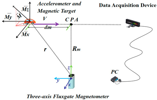
Figure 1. Magnetic target motion detection model.

To streamline the calculations, we use the center of the detection platform as the reference point and establish a three-dimensional Cartesian coordinate system with it as the coordinate origin. Assuming that the magnetic target moves along a straight path, we convert the target’s motion velocity into relative motion velocity with respect to the reference point. Thus, a magnetic dipole motion detection model is successfully established. In magnetic anomaly detection, adhering to the principles of magnetic dipole theory, we derive the vector expression of the magnetic induction intensity B at the detection platform’s location, as presented in Equation (1):

$$\mathbf{B}(\mathbf{M},\mathbf{r})=\frac{{\mu }_0}{4\pi }{r}^{-3}\left[\frac{3{\mathbf{r}}^{-2}(\mathbf{M}\cdot \mathbf{r})\mathbf{r}}{|\mathbf{r}{|}^5}-\frac{\mathbf{M}}{|\mathbf{r}{|}^5}\right]$$

(1)

where ${\mu }_0=4\pi \times {10}^{-7} \mathrm{H}/\mathrm{m}$ denotes the vacuum permeability, and $\mathbf{r}={\left[\begin{array}{ccc}x& y& z\end{array}\right]}^T$ represents the position vector of the dipole. The magnetic field generated by the magnetic target at the detection platform can be decomposed into three orthogonal axis directions of magnetic fields: $B_x$, $B_y$, and $B_z$. This magnetic field is influenced by the three-dimensional magnetic moment $M(M_x,M_y,M_z)$ of the target, which can be expressed as the three-dimensional magnetic moment of the magnetic target and the relative position between the magnetic target and the magnetic acquisition system. Then, the three-dimensional magnetic field generated by the magnetic target at the detection platform can be expressed by the three-dimensional magnetic moment and the relative position between the target and the detection platform, as illustrated in Equation (2):

$$\left[\begin{array}{c}{B}_x\\ B_y\\ B_z\end{array}\right]=\left[\begin{array}{ccc}3x^2-r^2& 3xy& 3xz\\ 3xy& 3y^2-r^2& 3yz\\ 3xz& 3yz& 3z^2-r^2\end{array}\right]\left[\begin{array}{c}{M}_x\\ M_y\\ M_z\end{array}\right]$$

(2)

where $r=\sqrt{x^2+y^2+z^2}$, and ${\left[\begin{array}{ccc}{B}_x& B_y& B_z\end{array}\right]}^T$ denote the components of $B$ along the three orthogonal directions.

Figure 2 shows the relationship between the magnetic field generated by the magnetic target at the detection platform and the geomagnetic field. The magnetic field generated by the magnetic target at the detection platform is $B$, the geomagnetic field at the detection platform is $B_{\mathrm{E}}$, and the geomagnetic field can be considered to be uniformly distribution in a narrow range. The total magnetic field measured using a magnetometer on the detection platform is $B_{\mathrm{S}}$, which is synthesized with the constant geomagnetic field part $B_{\mathrm{E}}$, and the magnetic anomaly field $B$, as shown in Equation (3).

$$B_{\mathrm{S}}=B+B_{\mathrm{E}}$$

(3)

where $\phi$ is the vector angle between the magnetic anomaly field $B$ and the geomagnetic field $B_{\mathrm{E}}$. In general, the value of the magnetic field $\left|B\right|$ of the magnetic target at the detection platform is about a few hundred nT, while the value of the geomagnetic field $\left|B_{\mathrm{E}}\right|$ is about 50,000 nT. When $|B|\ll |B_{\mathrm{E}}|$, the relationship between the total magnetic field, the anomalous magnetic field, and the geomagnetic field can be approximated as

$$\left|B_S\right|\approx \left|B_E\right|\times [1+\frac{1}{2}\left({\left|B\right|}^2+2\left|B_E\right|\times \left|B\right|\cos \phi \right)/{\left|B_E\right|}^2]$$

(4)

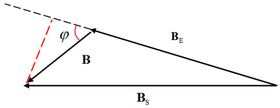
Figure 2. Relationship between the magnetic field $B$ of the magnetic target and the geomagnetic field $B_E$.

According to (3) and (4), the magnetic anomaly signal S at the detection platform obtained by the measurement is:

$$S=|B|-|B_{\mathrm{E}}|\approx \frac{B\cdot B_{\mathrm{E}}}{|B_{\mathrm{E}}|}=|B|\cos \phi =B\cdot i_e$$

(5)

where $i_e$ is the unit vector in the direction of the geomagnetic field. It can be seen from Equation (5) that the measured magnetic anomaly signal of the magnetic target at the detection platform is the projection of the magnetic anomaly field generated by the magnetic target at the detection platform in the direction of the geomagnetic field.

2.2. Standard Orthogonal Basis Decomposition

The standard orthogonal basis serves as a method to dissect magnetic anomaly signals. It seeks to decompose the magnetic field, under the framework of the target magnetic dipole model, into several orthogonal basis functions. Subsequently, energy detection is achieved by summing up the squares of the weighted coefficients. Within this method, magnetic anomaly signals manifest as a linear combination of three distinct functions, depicted in Equation (6):

$$S=\frac{\mu M}{4\pi R_m^3}{\displaystyle \sum _{n=1}^3{\tau }_n{\phi }_n(w)}$$

(6)

where ${\tau }_n$ symbolizes the coefficient of the basis functions, with $w$ equating to $dm/Rm$. The foundational basis functions are classified as ${\phi }_1(w)=\frac{w^2}{{[1+w^2]}^{\frac{5}{2}}}$, ${\phi }_2(w)=\frac{w}{{[1+w^2]}^{\frac{5}{2}}}$, and ${\phi }_3(w)=\frac{1}{{[1+w^2]}^{\frac{5}{2}}}$. After undergoing Schmidt orthogonalization and normalization, the following orthogonal basis functions emerge:

$$f_1(w)={\phi }_1(w)\sqrt{\frac{128}{3\pi }}, f_2(w)={\phi }_2(w)\sqrt{\frac{128}{5\pi }}, \mathrm{and} f_3(w)=\left[{\phi }_3(w)-\left(\frac{5}{3}\right){\phi }_1(w)\right]\sqrt{\frac{24}{5\pi }}.$$

These functions have orthogonality and normalization properties, as illustrated in Equation (7):

$$\{\begin{array}{c}{\displaystyle {\int }_{-\infty }^{+\infty }{f}_1(w)f_j(w)dw=0,i\ne j}\\ {\displaystyle {\int }_{-\infty }^{+\infty }{f}_1^2(w)dw=1,i=1,2,3}\end{array}$$

(7)

Relying on the orthogonality of the OBF, the decomposition coefficients ${\tau }_1$, ${\tau }_2$, and ${\tau }_3$ are derived from the orthogonal basis decomposition, with their respective solution formulas presented as:

$${\tau }_n={\left(\frac{{\mu }_{0}M}{4\pi R_m^3}\right)}^{-1}{\displaystyle {\int }_{-\infty }^{+\infty }{f}_n(w)Sdw}, n=1,2,3$$

(8)

During real-time magnetic target detection, the magnetic anomaly signal $S$ is contemporaneously measured with discrete values. The timeliness of this signal is pivotal. To uphold this real-time characteristic of the magnetic anomaly signal $S$, one can employ a sliding time window for decomposition. This process is visually represented in Figure 3.

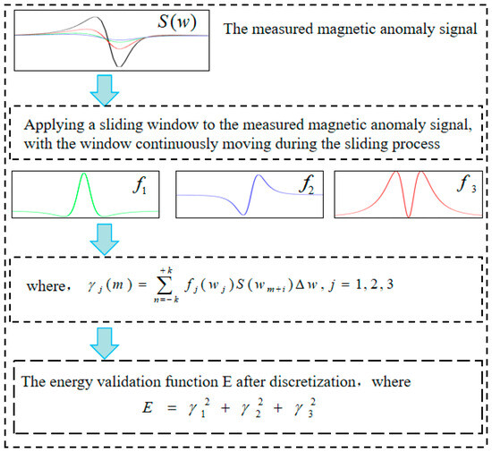
Figure 3. Process of the discrete orthogonal basis decomposition.

2.3. Establishment of the $\beta -OBF$ Relationship

Within the conventional OBF decomposition detection framework, the pivotal determinant is the selection of w, where $w$ equals $d_m/Rm$. Consequently, the cruising relative speed between the magnetic target and the detection platform emerges as a decisive factor for OBF decomposition detection. To establish the $\beta$-OBF relationship, one can start with an initial velocity v and adaptively acquire the optimal scale factor $\beta$. This is conducted to optimize the energy detection, considering that w aligns with $d_m/Rm$, where, $d_m=v\cdot t$.

From this foundation, let us evolve $w=\frac{d_m}{\sqrt{R_m^2+d_m^2}}$ to obtain Equation (9):

$$w=\sqrt{\frac{d_m^2}{R_m^2+d_m^2}}$$

(9)

Upon conducting appropriate transformations, we can derive Equation (10):

$$w={\left[1+\frac{R_m^2}{d_m^2}\right]}^{-\frac{1}{2}}$$

(10)

Further simplification via the Taylor series expansion [17] leads to Equation (11):

$$w=\left[1-\frac{R_m^2}{2d_m^2}\right]+o{(\frac{R_m^2}{d_m^2})}^2$$

(11)

We can further improve this to obtain Equation (12):

$$w=\left[1-\frac{R_m^2}{2(\beta \cdot v\cdot t{)}^2}\right]w\in \left[\begin{array}{cc}-\infty & +\infty \end{array}\right]$$

(12)

3. Establishment of the Scale Factor Model

3.1. Magnetic Dipole Model Simulation

Presuming the magnetic moment of the target is defined as $M$ = $(0,0,330)$$\mathrm{A}\cdot {\mathrm{m}}^2$, and the sampling frequency is denoted by $Fs$ = 50 $\mathrm{Hz}$, the simulation casts the magnetic target in a stationary role while the detection platform propels at a relative speed of $v=0.4 \mathrm{m}/\mathrm{s}$. The minimal distance from the center of the detection platform to the magnetic target is $Rm=2 \mathrm{m}$, while the detection platform traverses a span of $50 \mathrm{m}$. A visual representation of the three-dimensional model is unveiled in Figure 4.

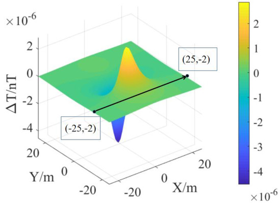
Figure 4. Three−dimensional model schematic.

Extracting the magnetic anomaly signal from the three-dimensional model, the magnetic anomaly signals of the magnetic field’s three components and the total magnetic field are extracted, as shown in Figure 5.

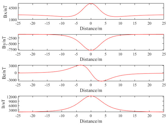
Figure 5. The magnetic field components of the magnetic dipole model.

3.2. Finite Element Method Simulation Models

According to the same simulation conditions of the magnetic dipole model, a rectangular permanent magnet with dimensions of 20 cm × 10 cm × 5 cm was selected as the magnetic target. In order to calculate the magnetic field in the entire space accurately, the finite element simulation software COMSOL Multiphysics 6.0 was utilized to establish the model. The material properties of the magnetic target were set as iron with a relative magnetic permeability of ${\mu }_0=4\pi \times {10}^{-7}\mathrm{H}/\mathrm{m}$ (since the propagation characteristics of static magnets in air and water are essentially the same). The background magnetic field was set as the geomagnetic vector for the Xi’an region [41,529 −1218 2183]nT (in the north-east-down coordinate system) to simulate the surrounding environment of the magnetic target. Figure 6 illustrates the geometric model of the permanent magnet.

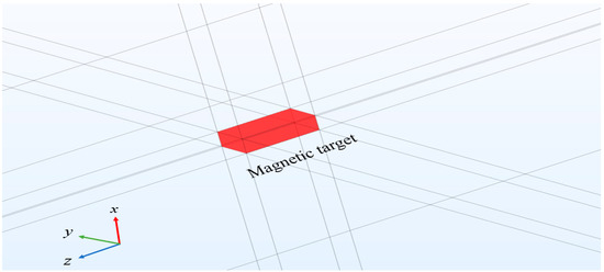
Figure 6. Geometrical model of the magnetic target.

After completing the geometric modeling of the permanent magnet body, the next step was to model the surrounding computational space. The dimensions of this computational space were 20 m × 10 m × 5 m, as shown in Figure 7.

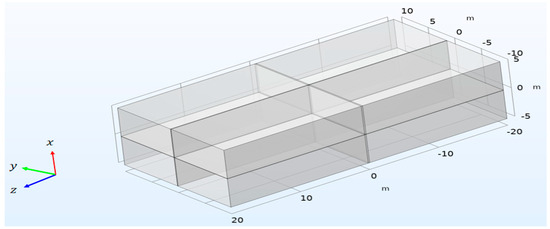
Figure 7. The geometric model diagram of the air domain.

The three components of the magnetic field at $Rm=2 \mathrm{m}$ are illustrated in Figure 8.

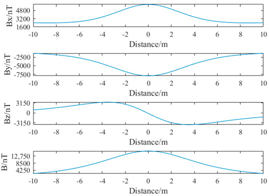
Figure 8. Three components of the magnetic field.

Based on the simulation results of these two models, we concluded that both models demonstrate similar effectiveness in reflecting magnetic anomaly signals under the experimental conditions. However, considering that the magnetic dipole model is a simple and widely used target model with specific expressions for the radiation field, it has been extensively applied. Therefore, in engineering practice, within a spatial range greater than 2.5 times the length of the magnetic target, the magnetic target can be treated as a magnetic dipole for analysis, which is more practically meaningful.

3.3. Magnetic Anomaly Simulation Based on Unknown Velocity

Harnessing the traditional orthogonal basis decomposition technique and assigning arbitrary relative velocity $v$, within the predefined conditions, we introduced velocity perturbations anchored to the set speed. This was followed by orthogonal basis detection. The velocity perturbation curve is visually portrayed in Figure 9; Figure 10 delineates the detection curve.

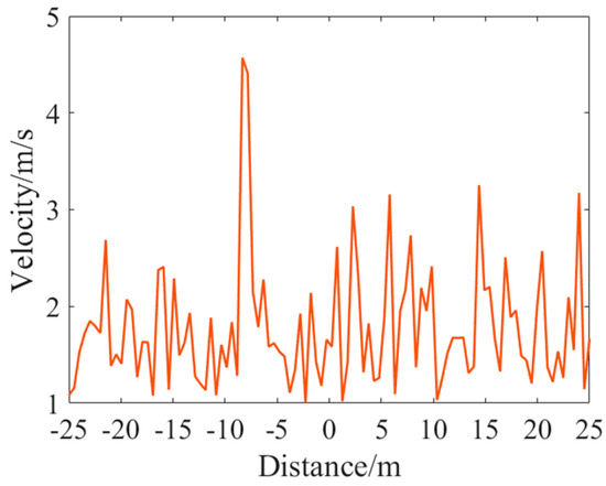
Figure 9. Velocity perturbation curve.

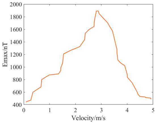
Figure 10. v−Em energy detection curve.

From the simulation results, it is discernible that traditional methods fall short in maximizing energy detection subsequent to orthogonal basis decomposition, especially when crossing the CPA. This revelation underscores the limitations of traditional methods. Consequently, a pressing need emerges to reimagine, refine, and elevate the orthogonal basis decomposition technique to ensure enhanced efficacy.

3.4. Monte Carlo Verification of Scale Factors under Orthogonal Basis Functions

In the conditions mentioned earlier, a simulation with 50 sets of different velocities $v$ with perturbations was conducted. These velocities were then incorporated into the modified orthogonal basis function variables for testing. In the $\beta -\mathrm{O}\mathrm{B}\mathrm{F}$ relationship, we identified the variable w corresponding to two different receiver operating characteristic (ROC) curves. These results are illustrated in Figure 11.

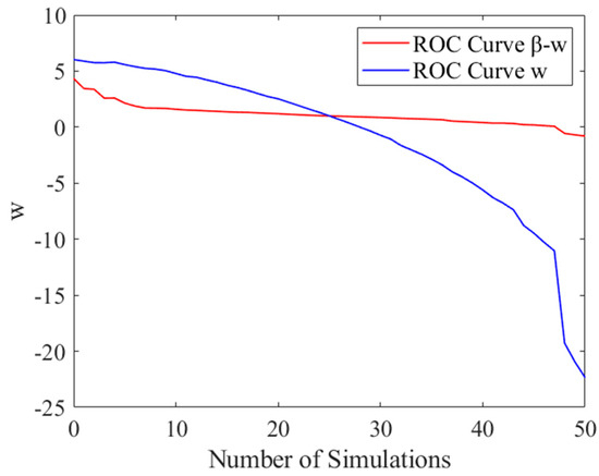
Figure 11. ROC−w function detection curves.

Among these, the conventional orthogonal basis functions exhibit significant variability in the independent variables. However, the modified orthogonal basis decomposition, characterized by the independent variable $\beta -w$, demonstrates greater stability. Following this assertion, the distribution of the aforementioned detection curves was simulated by generating 1000 sets of random data. The Monte Carlo method was employed to validate and assess the independent variables $w$ and $\beta -w$ within the orthogonal basis functions. The model’s generalization capability was estimated using random sampling. The $\beta -w$ detection curve exhibits superior generalization performance. The evaluation curve is depicted in Figure 12.

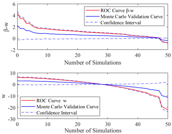
Figure 12. Monte Carlo evaluation curve.

3.5. Simulation of Scale Factors in Magnetic Anomaly Detection

Building upon the previous simulation, it was observed that when the magnetic target passes the CPA, the energy detection does not reach its maximum peak without the optimal scale factor $\beta$. To address this issue, further simulations were conducted, selecting 50 different $\beta$ values. The maximum orthogonal basis energy value $E$ was found at a velocity of $v=2 \mathrm{m}/\mathrm{s}$. Figure 13 provides a schematic representation of $\beta$ from the simulations, offering essential insights into the scale factor.

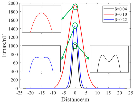
Figure 13. Maximum energy detection Emax for optimal β.

Recording the current velocity along with its corresponding scale factor, we conducted simulations to determine the optimal energy solution under 50 different velocities. Subsequently, we attempted to use various curve-fitting models. Upon comparing the fitting performance, it became evident that the Gauss model exhibited the lowest root mean square error and residual sum of squares, signifying the best fitting performance. The data for the evaluation are presented in Table 1.

Table 1. Gauss model evaluation data.

Fitting Category/ Fitting Metric	SSE	R-Square	RMSE
Power model	0.01889	0.9734	0.02049
Sum of sine model	0.09545	0.8654	0.02049
Weibull model	0.07372	0.8961	0.04003
Gauss model	0.01309	0.9815	0.01765

The fitting function using the Gauss model is:

$$\begin{array}{l}\beta (v)=k_1\cdot \exp \left(-{\left(\frac{(x-k_2)}{k_3}\right)}^2\right)+k_4\times \exp \left(-{\left(\frac{(x-k_5)}{k_6}\right)}^2\right)\\ \begin{array}{cc}{k}_1=0.8174& w_1(-0.1119,1.747)\end{array}\\ \begin{array}{cc}{k}_2=-0.1933& w_2(-0.9393,0.5528)\end{array}\\ \begin{array}{cc}{k}_3=0.6701& w_3(0.2754,1.065)\end{array}\\ \begin{array}{cc}{k}_4=2.153e13& w_4(-1.28e17,1.289e17)\end{array}\\ \begin{array}{cc}{k}_5=-314.4& w_5(-5.791e4,5.728e4)\end{array}\\ \begin{array}{cc}{k}_6=55.26& w_6(-4958,5069)\end{array}\end{array}$$

(13)

where $k_i(i=1,2,\dots ,6)$ represents coefficients in the model, indicating the magnitudes of the exponential and constant terms, and $w_i(i=1,2,\dots ,6)$ represents their confidence intervals. The Gauss curve is depicted in Figure 14.

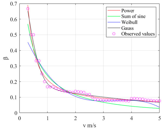
Figure 14. Fitting Gauss curves of scale factor and velocity matching under different methods.

3.6. Time Alignment Simulation of $\beta$

Based on the Gauss curve obtained from the simulation, a velocity of 1.5 $\mathrm{m}/\mathrm{s}$ was set. Using this velocity value, we calculated the corresponding $\beta$ and plotted the orthogonal basis energy curves. Figure 15 displays the new orthogonal basis energy curve and the traditional orthogonal basis curve.

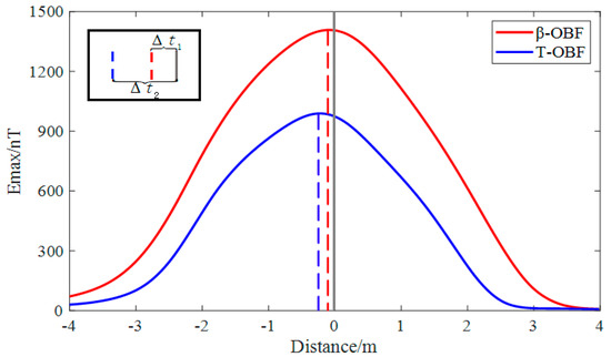
Figure 15. Orthogonal basis energy values.

In Figure 15, $\Delta t_1$ and $\Delta t_2$ represent the time difference of the peak of orthogonal basis energy achieved by the adaptive scale factor $\beta$ and the conventional OBF method, respectively. Research indicates that the meticulous selection of the adaptive scale factor $\beta$ markedly enhances the time alignment between the peak of orthogonal basis energy and the theoretical result, leading to a more precise time synchronization. The data of orthogonal basis energies are shown in Table 2.

Table 2. Orthogonal basis energy data.

	Emax/nT	Distance/m	V m/s	$\mathbf{\Delta }\mathit{T}$
OBF	885	0.24	1.5	0.164
$\beta$-OBF	1233	0.11	1.5	0.073

Based on the bias analysis of the above data, the following conclusions were drawn:

(1)

The peak value that can be achieved with OBF detection under the traditional approach is 885 nT, while the peak value of the adaptive scale factor β-OBF detection is 1233 nT. In comparison, the adaptive scale factor approach improves the peak value by 39.3%.

(2)

In the OBF detection method under the traditional approach, the deviation $\Delta t_2$ at the peak of the near CPA is 0.164, while the deviation $\Delta t_1$ of the scale factor β-OBF at the peak of the near CPA is 0.073, which is improved by 55.4% compared with that of the traditional approach.

The comprehensive simulation results show that the proposed method using Gaussian curve fitting can accurately determine the optimal scale factor β at a specific speed, thus maximizing the energy peak in the detection of magnetic anomaly signals. Additionally, this method improves the detection probability of magnetic anomaly signals of the acquisition device under an unknown motion state. The method significantly optimizes the matching of the moment of passing CPA at a simulated speed with that of the theoretical moment.

4. Experiment

For this experiment, we selected an expansive outdoor area with open space, a uniform and stable geomagnetic magnetic field, and no interference sources. The equipment utilized in the field experiment is illustrated in Figure 16. The experimental setup comprised a three-axis fluxgate magnetometer, an electronically controlled small car, and a magnetic acquisition device. Within the electronically controlled car, a $\text{Rb-Fe-B}$ magnet and a six-axis accelerometer were positioned. The car could move at a uniform velocity, with velocity adjustments possible. The orientation of the magnetic moment of the magnet and the fluxgate magnetometer is depicted in Figure 16 (3). (Assistance from a person was required when the speed was low.)

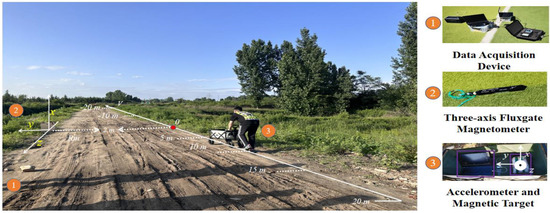
Figure 16. Environment and equipment of experiment.

The magnitude of the magnetic moment was 330 $\mathrm{A}\cdot {\mathrm{m}}^2$. The car moved at a lateral distance of $Rm=2\mathrm{m}$ from the three-axis fluxgate magnetometer, maintaining uniform speeds of $0.5\mathrm{m}/\mathrm{s}$, $1.5\mathrm{m}/\mathrm{s}$, and $2.7\mathrm{m}/\mathrm{s}$, respectively. Figure 17 displays the total field and the three components of the magnetic anomaly measurement signals obtained after calibration.

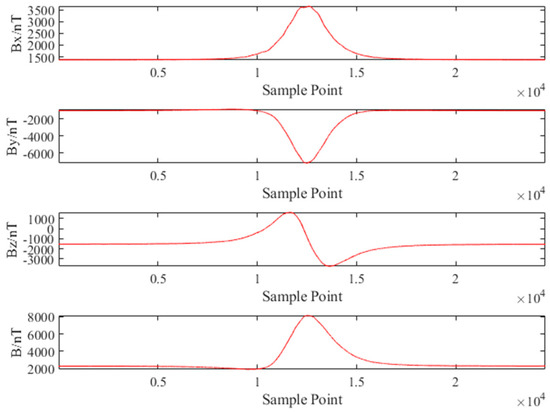
Figure 17. The total field and the three components of the magnetic anomaly measurement signals obtained after calibration: raw data after sensor calibration.

Considering velocity error, we conducted experiments at each velocity five times. To gauge the velocity at each time interval, we employed an accelerometer and analyzed the data with a velocity error within a $10\%$ range, as presented in Figure 18.

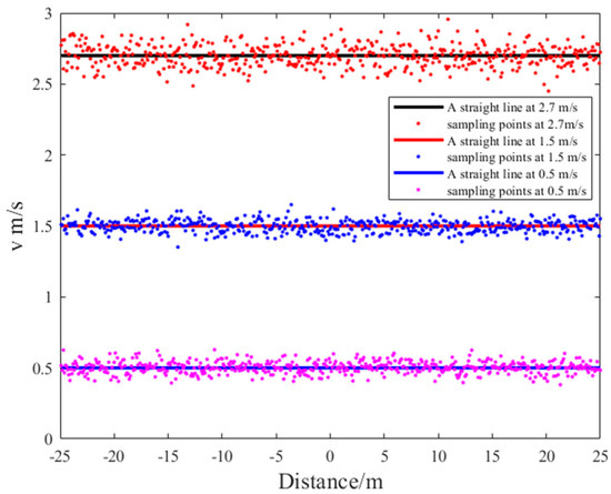
Figure 18. Sampling points of different velocities.

By conducting comprehensive tests and precise accelerometer measurements, it was possible to gain deeper insights into speed variations in practical situations and to minimize the influence of random error. This data acquisition approach offers enhanced reliability and facilitates a more accurate analysis. The adaptive scale factor method ultimately aims to elevate the precision and dependability of detection for an unknown magnetic target motion state. Leveraging the experimental data, we performed orthogonal basis decomposition of the magnetic anomaly total field signals and determined the optimal scale factor $\beta$. This process yielded energy measurements from orthogonal basis decomposition at various velocities, as depicted in Figure 19.

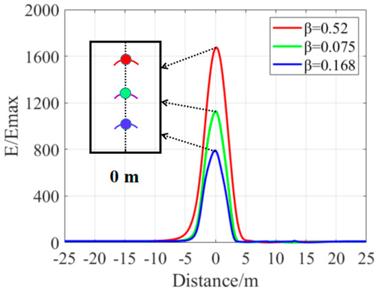
Figure 19. Energy measurements from orthogonal basis decomposition at different velocities.

In the comparative analysis, we used the OBF with a scale factor β = 0.075 for the speed of 1.5 m/s and compared it with the conventional OBF detection method. Figure 20 shows a comparison of the results.

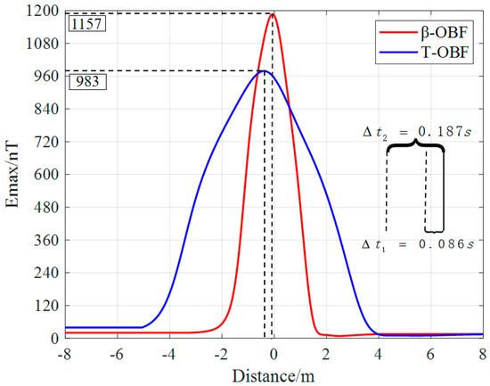
Figure 20. Comparative analysis of T−OBF and β-OBF at 1.5 m/s: evaluating performance and results.

The following conclusions can be drawn from the data in Figure 20:

(1)

In the experiment, the peak energy value that could be achieved with the traditional approach was 983 nT; the adaptive scale factor β-OBF detection obtained a peak energy value of 1157 nT. In comparison, the adaptive scale factor approach improved the peak value by 17.7%.

(2)

Using the OBF detection method with the conventional approach, the deviation t2 at the peak near the CPA was 0.187 s, while the deviation t1 of the scale factor β-OBF at the peak near the CPA was 0.086 s, which was an increase in accuracy 54.1%.

The adaptive scale factor method proposed in this paper shows obvious advantages in improving magnetic anomaly signal detection. The experimental results show that the adaptive scale factor method significantly improves the value of peak energy compared to that of the conventional approach. In addition, the adaptive scale factor method achieves better performance in terms of the deviation at the peak value near the CPA. The effectiveness and precision of the proposed method in practical applications were verified through experiments. Therefore, this study provides a new idea and method for magnetic detection technology, which shows important practical application value.

5. Conclusions

This paper introduces an adaptive scale factor method derived from orthogonal basis function decomposition. This method addresses the challenges faced by the OBF detector in conventional magnetic anomaly detection, particularly when confronted with unknown relative velocities or non-ideal uniform motion. In simulations, we employed techniques to adjust the relative velocity between the detection platform and the magnetic target, along with modifying the characteristic time. By constructing a viable mathematical model and fitting it to a Gauss function curve, we achieved adaptive detection of magnetic anomaly signals under an unknown motion state. In the context of non-ideal uniform motion, an adaptive selection of the optimal scaling factor β is employed based on measured data under unknown velocity states. This approach aims to enhance the output signal-to-noise ratio of magnetic anomaly targets in non-ideal conditions. Furthermore, the traditional orthogonal basis function decomposition energy value was effectively improved by 17.7%. Additionally, the time when the magnetic target passes through the closest point of approach (CPA) aligned with the peak of the orthogonal basis decomposition energy detection, resulting in a 54.1% increase in precision compared to the conventional method. Consequently, this enhancement significantly bolsters the detector’s performance. In conclusion, this method provides a new approach for the magnetic anomaly detection technology under an unknown motion state, which can improve the accuracy and performance of magnetic anomaly signal detection in practical applications. This method can also be applied to other fields of signal processing and target detection. Finally, the scale factor approach also provides reference and guidance for subsequent research. Therefore, this method is not only important for researchers in related fields but also provides a feasible improvement for practical applications.

References

- Clem, T.R. Sensor technologies for hunting buried sea mines. In Proceedings of the OCEANS’02 MTS/IEEE, Biloxi, MI, USA, 29–31 October 2002; Volume 1, pp. 452–460. [Google Scholar]
- Zhao, Y.; Zhang, J.H.; Li, J.H.; Liu, S.; Miao, P.X.; Shi, Y.C.; Zhao, E.M. A brief review of magnetic anomaly detection. Meas. Sci. Technol. 2021, 32, 042002. [Google Scholar] [CrossRef]
- Hirota, M.; Furuse, T.; Ebana, K.; Kubo, H.; Tsushima, K.; Inaba, T.; Shima, A.; Fujinuma, M.; Tojyo, N. Magnetic detection of a surface ship by an airborne LTS SQUID MAD. IEEE Trans. Appl. Supercond. 2001, 11, 884–887. [Google Scholar] [CrossRef]
- Smith, D.V.; Bracken, R.E. Field experiments with the tensor magnetic gradiometer system for UXO surveys: A case history. In SEG Technical Program Expanded Abstracts 2004; Society of Exploration Geophysicists: Houston, TX, USA, 2004; pp. 806–809. [Google Scholar]
- Nelson, J.B.; Richards, T.C. Magnetic Source Parameters of MR OFFSHORE Measured during Trial MONGOOSE 07; Defense R&D Canada-Atlantic: Ottawa, ON, Canada, 2007. [Google Scholar]
- Jin, H.; Guo, J.; Wang, H.; Zhuang, Z.; Qin, J.; Wang, T. Magnetic anomaly detection and localization using orthogonal basis of magnetic tensor contraction. IEEE Trans. Geosci. Remote Sens. 2020, 58, 5944–5954. [Google Scholar] [CrossRef]
- Ginzburg, B.; Frumkis, L.; Kaplan, B.Z. Processing of magnetic scalar gradiometer signals using orthonormalized functions. Sens. Actuators A Phys. 2002, 102, 67–75. [Google Scholar] [CrossRef]
- Sheinker, A.; Frumkis, L.; Ginzburg, B.; Salomonski, N.; Kaplan, B.-Z. Magnetic anomaly detection using a three-axis magnetometer. IEEE Trans. Magn. 2009, 45, 160–167. [Google Scholar] [CrossRef]
- Shen, Y.; Hasanyan, D.; Gao, J.; Wang, Y.; Li, J.; Viehland, D. A magnetic signature study using magnetoelectric laminate sensors. Smart Mater. Struct. 2013, 22, 095007. [Google Scholar] [CrossRef]
- Nazlibilek, S.; Ege, Y.; Kalender, O. A multi-sensor network for direction finding of moving ferromagnetic objects inside water by magnetic anomaly. Measurement 2009, 42, 1402–1416. [Google Scholar] [CrossRef]
- Shen, Y.; Wang, J.; Shi, J.; Zhao, S.; Gao, J. Interpretation of signature waveform characteristics for magnetic anomaly detection using tunneling magnetoresistive sensor. J. Magn. Magn. Mater. 2019, 484, 164–171. [Google Scholar] [CrossRef]
- Sheinker, A.; Moldwin, M.B. Magnetic anomaly detection (MAD) of ferromagnetic pipelines using principal component analysis (PCA). Meas. Sci. Technol. 2016, 27, 045104. [Google Scholar] [CrossRef]
- Wu, X.; Huang, S.; Li, M.; Deng, Y. Vector Magnetic Anomaly Detection via an Attention Mechanism Deep-Learning Model. Appl. Sci. 2021, 11, 11533. [Google Scholar] [CrossRef]
- Qin, Y.; Li, K.; Yao, C.; Wang, X.; Ouyang, J.; Yang, X. Magnetic anomaly detection using full magnetic gradient orthonormal basis function. IEEE Sens. J. 2020, 20, 12928–12940. [Google Scholar] [CrossRef]
- Liu, S.; Hu, J.; Li, P.; Wan, C.; Chen, Z.; Pan, M.; Zhang, Q.; Liu, Z.; Wang, S.; Chen, D.; et al. Magnetic anomaly detection based on full connected neural network. IEEE Access 2019, 7, 182198–182206. [Google Scholar] [CrossRef]
- Wang, Y.; Han, Q.; Zhao, G.; Li, M.; Zhan, D.; Li, Q. A deep neural network based method for magnetic anomaly detection. IET Sci. Meas. Technol. 2022, 16, 50–58. [Google Scholar] [CrossRef]
- Wang, G.; Zhu, H.; Guo, Z. Magnetic anomaly signal characteristics of ship induced magnetism. Ship Sci. Technol. 2015, 37, 137–139. [Google Scholar]
- Wang, S.; Zhang, M.; Zhang, N.; Guo, Q. Calculation and correction of magnetic object positioning error caused by magnetic field gradient tensor measurement. J. Syst. Eng. Electron. 2018, 29, 456–461. [Google Scholar]
- Mu, Y.; Wang, C.; Zhang, X.; Xie, W. A novel calibration method for magnetometer array in nonuniform background field. IEEE Trans. Instrum. Meas. 2018, 68, 3677–3685. [Google Scholar] [CrossRef]
- Chen, X.; Kong, X.; Xu, M.; Sandrasegaran, K.; Zheng, J. Road vehicle detection and classification using magnetic field measurement. IEEE Access 2019, 7, 52622–52633. [Google Scholar] [CrossRef]
- Chen, L.; Feng, Y.; Wu, P.; Zhu, W.; Fang, G. An innovative magnetic anomaly detection algorithm based on signal modulation. IEEE Trans. Magn. 2020, 56, 1–9. [Google Scholar] [CrossRef]
Disclaimer/Publisher’s Note: The statements, opinions and data contained in all publications are solely those of the individual author(s) and contributor(s) and not of MDPI and/or the editor(s). MDPI and/or the editor(s) disclaim responsibility for any injury to people or property resulting from any ideas, methods, instructions or products referred to in the content. |
© 2024 by the authors. Licensee MDPI, Basel, Switzerland. This article is an open access article distributed under the terms and conditions of the Creative Commons Attribution (CC BY) license (https://creativecommons.org/licenses/by/4.0/).