An Enhanced Aircraft Carrier Runway Detection Method Based on Image Dehazing

Abstract

Carrier-based Unmanned Aerial Vehicle (CUAV) landing is an extremely critical link in the overall chain of CUAV operations on ships. Vision-based landing location methods have advantages such as low cost and high accuracy. However, when an aircraft carrier is at sea, it may encounter complex weather conditions such as haze, which could lead to vision-based landing failures. This paper proposes a runway line recognition and localization method based on haze removal enhancement to solve this problem. Firstly, a haze removal algorithm using a multi-mechanism, multi-architecture network model is introduced. Compared with traditional algorithms, the proposed model not only consumes less GPU memory but also achieves superior image restoration results. Based on this, We employed the random sample consensus method to reduce the error in runway line localization. Additionally, extensive experiments conducted in the Airsim simulation environment have shown that our pipeline effectively addresses the issue of decreased detection accuracy of runway line detection algorithms in haze maritime conditions, improving the runway line localization accuracy by approximately 85%.

1. Introduction

Due to the needs of modern national security and interests development, aircraft carriers, as mobile platforms for aircraft takeoff and landing at sea, play a crucial role. Meanwhile, with the advancement of technology, whether in civilian or military scenarios, an increasing number of hardware devices are trending towards unmanned development. A CUAV deployed on ships, e.g., aircraft carriers and destroyers, is gradually playing vital roles in various aspects such as maritime rescue, reconnaissance, surveillance, target engagement, etc. Therefore, as a crucial aspect of the entire mission execution of shipborne CUAVs, CUAV landing has gradually become a popular research field in recent years. Typically, CUAV landing methods mostly rely on sensors such as vision, altitude, and laser, with vision sensors gradually becoming the most commonly used sensor type in this neighborhood due to their low cost and high accuracy [1]. One of the most crucial subtasks in landing missions is runway line detection and positioning.

For runway detection, there are in convention two kinds of methods, which are the traditional image processing methods [2,3] and deep learning methods [4,5]. Traditional image processing methods typically rely on image edge detection and often require the assumption of multiple ideal prior conditions, making them unsuitable for practical runway line detection. With the rapid advancements in neural networks over the past few years, runway detection algorithms for unmanned devices increasingly utilize convolutional neural network (CNN) algorithms. These algorithms [6,7,8,9] can achieve a well-generalized model by feeding a large amount of data into the network structure for forward propagation and then fine-tuning the model’s parameters through backpropagation using a loss function. In practical applications, these models are typically pruned and quantized before deployment onto hardware devices. They utilize camera data for inference to obtain reference results, enabling full process automation without human intervention in controlling device actions. Although these methods have achieved satisfactory runway detection results, carrier operations at sea often encounter adverse weather conditions such as rain and haze. This leads to degradation in the image data acquired by visual sensors, which inevitably affects the precision of CUAV runway detection. Undoubtedly, this increases the complexity and risk during CUAV landing missions.

In recent years, there has been a surge in work [10,11] on outdoor hazed image restoration. However, these methods often focus solely on the quality of image restoration without considering the feasibility of their practical application scenarios. This has led to an excessive number of model parameters and increased computational time for these methods.

This paper focuses on the problem of degradation in runway line recognition due to image sensor degradation in haze conditions and proposes a runway line recognition system based on image dehazing. In summary, the contributions of our paper can be mainly summarized as follows:

• A lightweight dehazing network that combines CNNs with Transformers structure is introduced. An effective complementary attention module and a novel Transformer of linear computation complexity are designed to enhance the network’s capability in image restoration;
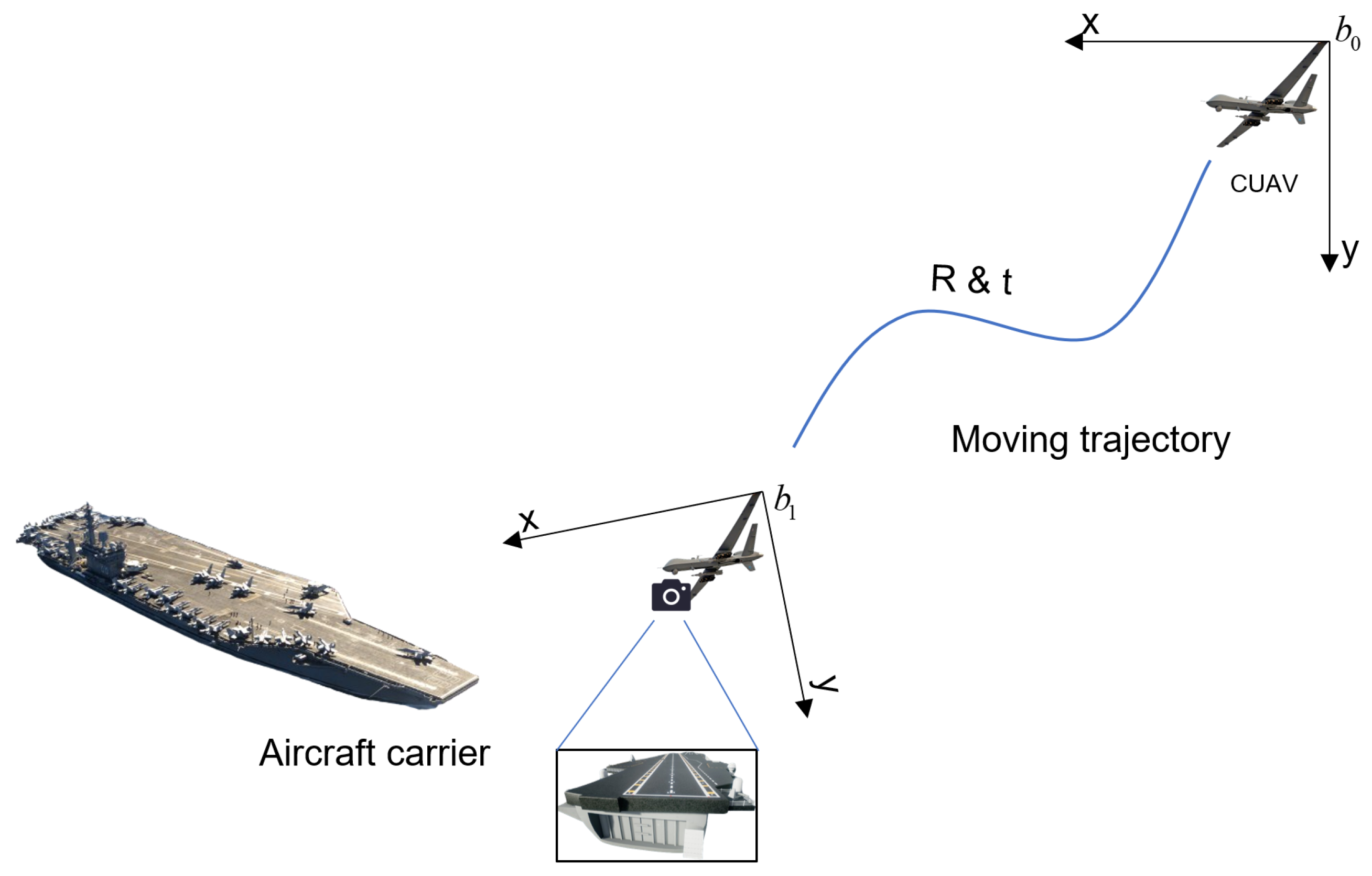
• By analyzing the positions of pixels obtained from the runway detection algorithm in two-dimensional space, adjusting the landing process of CUAVs by combining sensor data, performing multiple spatial transformations, and localization the spatial straight-line expressions of runway lines, a runway line localization method is proposed;
• A system framework is designed to address the issue of CUAVs experiencing difficulty in safely and reliably landing in hazed conditions at sea. In the Airsim simulation environment, we conduct extensive experiments. The result shows our system can effectively restore image content details and yield runway lines through localization with a deviation from ground truth of less than 2°.

In the remainder of the paper, we first discuss the related works in Section 2, followed by a detailed exposition of the methods and ideas adopted in the paper in Section 3. Subsequently, in Section 4, we conduct extensive experiments and analyze data to validate the effectiveness and feasibility of the proposed methods. Finally, in Section 5, we summarize the work conducted in the paper.

2. Related Work

In this section, we will primarily discuss the latest advancements in the fields of image dehazing and runway detection methods. We will elaborate on the relevant works proposed in recent years and summarize them separately in Table 1 and Table 2.

2.1. Image Dehazing

In convention, haze is viewed as a natural phenomenon that occurs when light interacts with particles in the atmosphere. The scattering of light by particles in the atmosphere causes the light to be scattered in all directions, resulting in a decrease in the contrast of the image [12]. In 1976, McCartney [13] first proposed the basic Atmospheric Scattering Model (ASM) theory to approximately explain the principles of haze formation. Then, in 2003, Narasimhan [14] and Nayar [15] further developed the ASM that is currently widely used. In the early stages, dehazing algorithms were similar to other image restoration tasks such as denoising and deblurring, relying on prior-based approaches. These methods were based on assumptions and prior knowledge derived from statistical analysis of a large number of degraded images’ physical properties, which were then used to implement the algorithm’s effectiveness. For example, Ref. [16] proposes the Dark Channel Prior (DCP) method. It assumes the minimum intensity value in one local window of a three-channel image intended to be zero in the haze-free image, and based on it the medium transmission map, as well as the global atmospheric light A, is estimated. Ref. [17] introduces a single-image dehazing method utilizing color-lines regularity and an augmented Markov random field model, significantly improving transmission accuracy and haze-free radiance recovery. Ref. [18] introduces the Rank-one Prior (RP) method, which proposes that the medium transmission map t as a rank-one matrix can be estimated by intensity projection strategy. Ref. [19] builds a color attenuation prior to haze removal from a single image, enabling the creation of a linear model for scene depth estimation and significantly enhancing dehazing efficiency and effectiveness compared to state-of-the-art algorithms. However, these methods are not robust enough to handle complex scenes and are sensitive to the choice of parameters.

Table 1. Summary of image dehazing methods.

Citation	Method	Category	Characteristics
[16]	Dark Channel Prior (DCP)	Prior-based	Based on assumptions and prior knowledge derived from statistical analysis of a large number of degraded images’ physical properties. It requires multiple iterations of calculations, can only handle images under specific hypothetical conditions, and has high computational complexity with limited satisfactory results.
[17]	Color-lines regularity and an augmented Markov random field model
[19]	Color attenuation prior
[18]	Rank-one Prior (RP)
[20]	estimating transmission matrix t by CNN	CNN	With a sufficient amount of synthetic image pairs, these can achieve superior dehazing results over traditional methods. However, due to the limited receptive field of CNN, which only captures spatially local features, it is challenging to obtain long-range dependencies of pixels.
[21]	predicting A and t by CNN
[22]	end-to-end neural network
[23]	end-to-end neural network
[24]	CNN and conventional Transformer fusion	Transformer	Compared to traditional CNN algorithms, this method achieves better image restoration metrics and generalization ability through multi-head self-attention computation. However, traditional Transformer based image dehazing methods are computationally intensive and a higher risk of overlocalization.
[10]	Swin Transformer
[25]	Image Processing Transformer (IPT)

Table 1. Summary of image dehazing methods.

Citation	Method	Category	Characteristics
[16]	Dark Channel Prior (DCP)	Prior-based	Based on assumptions and prior knowledge derived from statistical analysis of a large number of degraded images’ physical properties. It requires multiple iterations of calculations, can only handle images under specific hypothetical conditions, and has high computational complexity with limited satisfactory results.
[17]	Color-lines regularity and an augmented Markov random field model
[19]	Color attenuation prior
[18]	Rank-one Prior (RP)
[20]	estimating transmission matrix t by CNN	CNN	With a sufficient amount of synthetic image pairs, these can achieve superior dehazing results over traditional methods. However, due to the limited receptive field of CNN, which only captures spatially local features, it is challenging to obtain long-range dependencies of pixels.
[21]	predicting A and t by CNN
[22]	end-to-end neural network
[23]	end-to-end neural network
[24]	CNN and conventional Transformer fusion	Transformer	Compared to traditional CNN algorithms, this method achieves better image restoration metrics and generalization ability through multi-head self-attention computation. However, traditional Transformer based image dehazing methods are computationally intensive and a higher risk of overlocalization.
[10]	Swin Transformer
[25]	Image Processing Transformer (IPT)

In recent years, with the development of deep learning, the application of neural networks in image dehazing has become increasingly popular. Dehazenet [20] firstly carries out convolutional neural networks(CNNs) to forecast t. DCPND [21] simultaneously predicts A and t by ustilizing CNNs. AOD-Net [22] performs a dehazing network that simplifies the image dehazing process by directly generating clean images without separately estimating the transmission matrix and atmospheric light, demonstrating superior performance and fast processing speed. Ref. [23] proposes an end-to-end trainable neural network for single-image dehazing that leverages a fusion strategy to blend multiple derived inputs from the original hazy image, eliminating the need to explicitly estimate transmission and atmospheric light. However, due to the limited receptive field of CNN, which only captures spatially local features, it is challenging to obtain long-range dependencies of pixels which is vital for image dehazing. Some works on account of Transformers have also been introduced. Such as DeHamer [24] combines the CNN and conventional Transformer for image dehazing, DehazeFormer [10] utilizes the modified Swin Transformer [26] key structure enabling the elasticity for image dehazing. Ref. [25] introduces an Image Processing Transformer (IPT), a pre-trained model designed specifically for low-level vision tasks such as denoising, super-resolution, and deraining, leveraging a large-scale dataset and a multi-head, multi-tail architecture to achieve state-of-the-art performance across various benchmarks. This method is based on a transformer architecture and achieves excellent image restoration by processing the global and wide-range associative information in the image, refining the results from coarse to fine. Also, there exist works like MixDehazeNet [11] mix multiple attention mechanisms, such as channel attention, pixel attention, etc., diversiform kernel sizes, to achieve state-of-the-art (SOTA) performance in image dehazing. Although these algorithms achieve better hazing removal results compared to classical methods based on prior estimation, they still face two challenges: Firstly, they may not adapt well to complex real-world hazed image processing, and in some cases, they may even struggle to effectively restore certain artificial hazed images. Secondly, despite the proposal of diverse network modules and ongoing technological iterations, the parameter volume of network models continues to increase. In our work, we aim for the network to maintain a relatively small parameter volume while still delivering excellent hazed image restoration results.

2.2. Runway Detection

The runway detection method is a crucial part of the autonomous driving system. It is mainly divided into three categories: classification-based, object detection-based and segmentation-based methods [27]. Classification-based methods like DeepLanes [6], assume some location-dependent prior knowledge is datum and based on it to design a CNN architecture. Object detection-based methods like EELane [7] propose an empirical evaluation framework that integrates large-scale data collection with deep learning algorithms to achieve real-time vehicle and lane detection. VPGNet [8] proposes a VPGNet architecture that integrates a vanishing point prediction task to enhance the robustness of lane and road marking detection under various weather and illumination conditions, setting a new benchmark for multi-task learning in autonomous driving scenarios. STLNet [9] introduces a spatiotemporal deep learning approach for real-time lane detection that leverages both spatial and temporal constraints to enhance accuracy and robustness under various weather and traffic conditions. The aforementioned algorithms successively addressed the limitations of previous ones. Despite achieving satisfactory runway detection performance, the effectiveness and robustness are somewhat compromised by the constraints imposed by the inverse perspective transformation (IPM) process during post-processing. Segmentation-based methods like [28] perform a CNN-based regression approach for multilane detection and classification that focuses on producing parameterized lane information from image coordinates. Ref. [29] proposes a color-based segmentation approach for robust and efficient lane detection under various environmental conditions without relying on complex vision algorithms or extensive parameter tuning. Ref. [4] introduces a Spatial CNN (SCNN) architecture that enhances convolutional neural networks’ ability to capture spatial relationships between pixels for improved traffic scene understanding. Ref. [30] introduces a Recurrent Feature-Shift Aggregator (RESA) that leverages strong shape priors of lanes and captures spatial relationships of pixels across rows and columns through recurrent shifting of sliced feature maps, along with a Bilateral Up-Sampling Decoder for refining pixel-wise predictions in lane detection tasks. These methods typically operate on regions of individual pixels in the entire image, leveraging the paradigm of semantic segmentation to delineate runway lines within the image. In recent years, there have also been some row-based algorithms that assume a line of runway anchors in the fixed row direction. Such as, CLRNet [31] employs learnable anchor parameters, started from $x_0, y_0, {\theta }_0$, and runway length $l_0$. LaneFormer [32] introduces a novel Transformer with x and y axis attention mechanism to detect runway instances. UFLD [5] leverages the flattening operation to convert the 2D feature map into a 1D vector, and then the row-wise runway point positions are detected by the 1D feature map. In our work, we adopt the UFLD algorithm to detect runway lines in the images. The algorithm is lightweight and fast, which is suitable for real-time applications. In addition, for applications in hazed maritime scenarios, we have adjusted the confidence modification based on the quality of the dehazed images, altering the hyperparameters set during training. This enhancement aims to improve the detection robustness in haze conditions.

Table 2. Summary of lane detection methods.

Method	Method	Category	Characteristics
[6]	DeepLanes	classification-based	It get an advantage result of a complicated network structure. However, the prior position setting curbs its application in practical scenarios, and due to the complex network, the method is time-consuming.
[7]	EELane	Object detection-based	By labeling regression bounding boxes or feature points for each lane segment, lanes can be efficiently detected by coordinate regression. However, due to the inverse perspective transformation (IPM) process during post-processing, its robustness is conditioned.
[8]	VPGNet
[9]	STLNet
[28]	CNN-based regression approach	segmentation-based	These methods typically operate on regions of individual pixels in the entire image, leveraging the paradigm of semantic segmentation to delineate runway lines within the image. But segmentation paradigm is inherently too strict, and the emphasis is on obtaining accurate classification per pixel rather than specifying the shape.
[29]	color-based segmentation approach
[4]	Spatial CNN (SCNN)
[30]	Recurrent Feature-Shift Aggregator (RESA)
[31]	CLRNet	row-based	These methods use anchor point detection set along a specific direction of the image (e.g., row direction), thus achieving good runway line detection results and real-time detection speed. However, these methods are highly dependent on image quality, and their detection performance significantly degrades when the images are hazy.
[32]	LaneFormer
[5]	UFLD

Table 2. Summary of lane detection methods.

Method	Method	Category	Characteristics
[6]	DeepLanes	classification-based	It get an advantage result of a complicated network structure. However, the prior position setting curbs its application in practical scenarios, and due to the complex network, the method is time-consuming.
[7]	EELane	Object detection-based	By labeling regression bounding boxes or feature points for each lane segment, lanes can be efficiently detected by coordinate regression. However, due to the inverse perspective transformation (IPM) process during post-processing, its robustness is conditioned.
[8]	VPGNet
[9]	STLNet
[28]	CNN-based regression approach	segmentation-based	These methods typically operate on regions of individual pixels in the entire image, leveraging the paradigm of semantic segmentation to delineate runway lines within the image. But segmentation paradigm is inherently too strict, and the emphasis is on obtaining accurate classification per pixel rather than specifying the shape.
[29]	color-based segmentation approach
[4]	Spatial CNN (SCNN)
[30]	Recurrent Feature-Shift Aggregator (RESA)
[31]	CLRNet	row-based	These methods use anchor point detection set along a specific direction of the image (e.g., row direction), thus achieving good runway line detection results and real-time detection speed. However, these methods are highly dependent on image quality, and their detection performance significantly degrades when the images are hazy.
[32]	LaneFormer
[5]	UFLD

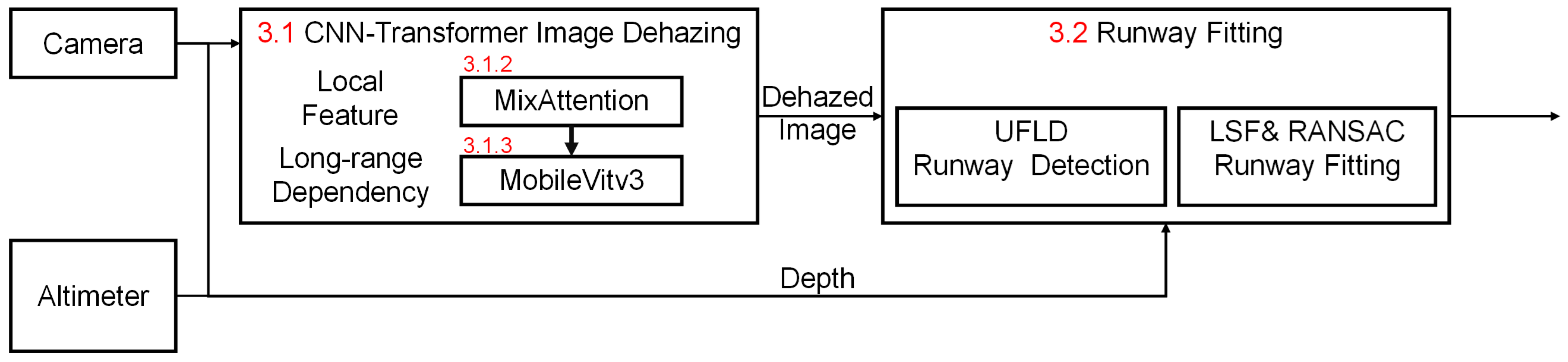
3. Materials and Methods

To enhance the airborne landing safety of carrier-based unmanned aerial vehicles in maritime hazed conditions, we have devised the method pipeline as illustrated in Figure 1. This pipeline primarily comprises three segments: image dehazing, runway line detection, and runway line localization, followed by the assessment of runway line localization error. Therefore, for a coherent exposition of our approach, this section predominantly expounds in three parts. Firstly, we provide a detailed analysis and explanation of the dehazing model architecture designed in this paper, along with each module. Secondly, we derive and elucidate the formulas for the runway localization method and error analysis adopted in this paper. In the end, we supplement the description of the environmental construction steps and data collection methods for the dataset used in this paper.

Figure 1. The overall pipeline framework.

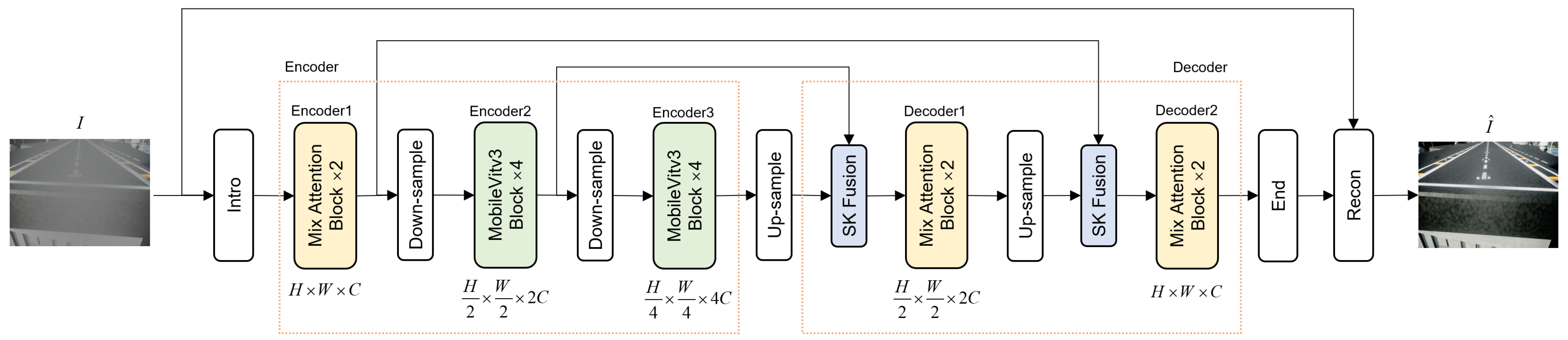
3.1. Dehaze Implementation

In this part, we first provide a detailed explanation of the overall workflow of the network, followed by descriptions of the structures and functions of each basic module used in the network.

3.1.1. Network Overall

The overall framework of the network, as depicted in Figure 2, comprises a U-shaped hierarchical structure consisting of symmetric encoders and decoders. The encoder is composed of down-sampling modules, MixAttention, and Mobilevit modules, while the decoder consists of up-sampling modules, MixAttention, and SKFusion [10] modules. Each level of the encoder and decoder has a skip connection. The SKFusion module fuses the input of each layer of the decoder with the output of the skip connection through the SKFusion module and passes it to the next layer. With each layer of down-sampling modules, the channel number of the feature map doubles while the spatial dimension halves. Conversely, with each layer of up-sampling modules, the channel number of the feature map halves while the spatial dimension doubles. For a hazed image $I\in {\mathbb{R}}^{H\times W\times 3}$, it first passes through an introduction module to obtain low-dimensional feature information $F_s\in {\mathbb{R}}^{H\times W\times C}$. Then, it undergoes a bottom-up encoding process to gradually obtain deep-level high-dimensional features $F_d\in {\mathbb{R}}^{\frac{H}{4}\times \frac{W}{4}\times 4C}$. Subsequently, it passes through a top-down decoder and a convolutional operation with a kernel size of $3\times 3$ to obtain residual features $F_{res}\in {\mathbb{R}}^{H\times W\times 4}$. Finally, $F_{res}$ is split into two feature maps, K and B, with different dimensionalities. Then, analogized by the classic Atmospheric Scattering Model theory, passing through element-wise multiplication between $K\in {\mathbb{R}}^{H\times W\times 1}$ and $B\in {\mathbb{R}}^{H\times W\times 3}$ to reconstruct the dehazed image $\widehat{I}$, i.e., $\widehat{I}=K\odot I-B+I$, ⊙ means the element-wise multiplication. For downsample operation and upsample operation, we implement convolution with a kernel size of 2 and a stride of 2 and Pixelshuffle PixelShuffle with an upsampling factor of 2, respectively.

Figure 2. Network architecture of the proposed model. The model is a modified 5-stage U-shape Net. The input shape is H ×W × C and the feature maps in each stage are shown below every block.

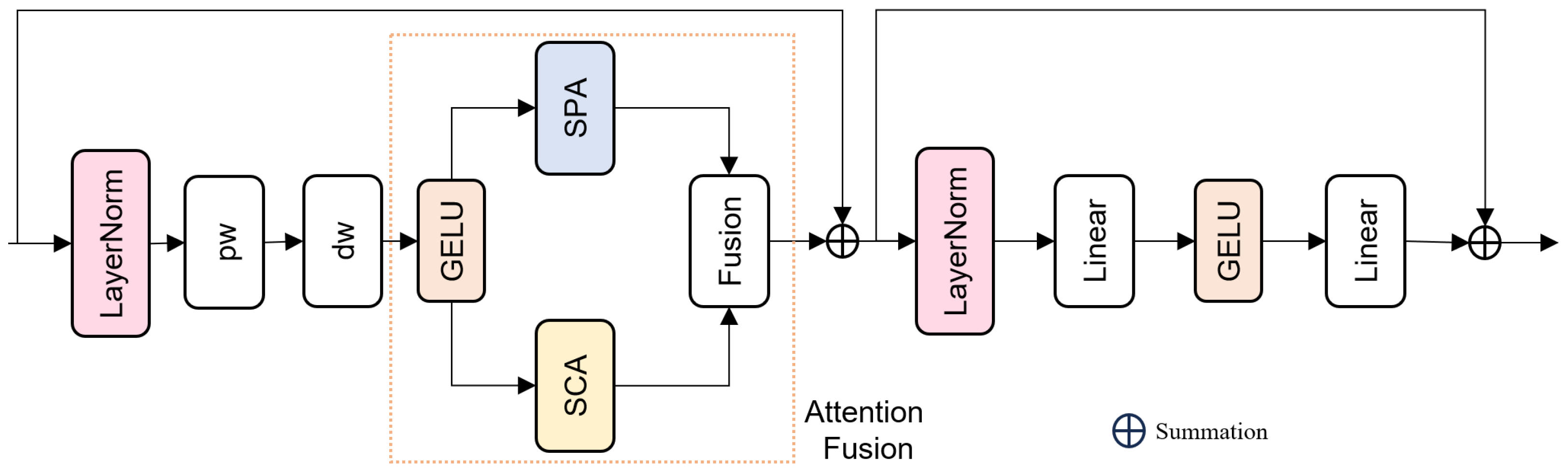
3.1.2. MixAttention Module

In hazed images, compared to clears, there are primarily two differences: decreased image contrast and loss of edge and texture information. To address these issues, we believe that appropriate attention modules should be employed to enable the network to selectively focus on specific information in the image. Inspired by recent advances in attention mechanisms in machine learning, we propose the MixAttention module. The module integrates both simple spatial attention (SPA), simple channel attention (SCA) mechanisms and feed-forward network (FFN), and fuses the feature information from these two attention modules through a linear mapping layer. The simple spatial attention mechanism primarily calculates cross-pixel attention weights for multi-dimensional features, emphasizing edges, textures, and dense blurry regions within the image. Meanwhile, the channel attention mechanism computes cross-channel attention weights for multi-dimensional features, focusing on color distribution characteristics within the image. The input of the MixAttention module undergoes Layer Normalization followed by respective processing through pixel-wise convolutional layers and depth-wise convolutional layers. Subsequently, after non-linear activation, the features are passed through SCA and SPA to obtain cross-channel and cross-pixel fusion feature information. After attention fusion, the FFN increases the dimensionality of the feature maps obtained through attention operations, applies non-linear activation functions, and then reduces the dimensionality to enhance feature representation capacity. The MixAttention model is shown in Figure 3.

Figure 3. The structure of MixAttention architecture. In the attention fusion part, it consists of two different attention mechanisms: SPA and SCA.

The implementation details of SPA and SCA can be found in Figure 4. From the figure, it can be observed that the attention computation of SPA and SCA are both divided into two branches. After element-wise multiplication, attention-weighted calculation output is obtained. The difference lies in the fact that when the feature map $F_{non}\in {\mathbb{R}}^{H\times W\times C}$ undergoes the non-linear branch of SCA, the shape of the feature map changes to ${\mathbb{R}}^C$, in contrast, SPA does not reshape. The SPA and SCA can be individually formulated as:

$$F_{spa}[h,w,k]=\sigma \left(\sum _{c=1}^{C}w\left(c\right)F_{non}[:,:,c+k]\right)\times \sum _{i=1}^H\sum _{j=1}^W\sum _{c=1}^{C}w[i,j,c]F_{non}[h+i,w+j,c+k],$$

(1)

$$F_{sca}[h,w,k]=\sigma \left(\sum _{c=1}^{C}w\left(c\right)\mathcal{P}\left(F_{non}[:,:,c+k]\right)\right)\times F_{non}[h,w,k],$$

(2)

where $\sigma$ denotes the Sigmoid activation function, × means the element-wise multiplication operation, $w\left(c\right)$ and $w[i,j,c]$ are the attention weights at point $[:,:,c]$ or $[i,j,c]$ of the channel and spatial attention mechanisms, respectively, $\mathcal{P}$ represents the global average pooling operation, $[h,w,k]$ is the pixel point coordinate of the feature map, and $F_{non}$ is the input feature map.

Figure 4. Implementation details of the SPA and SCA module.

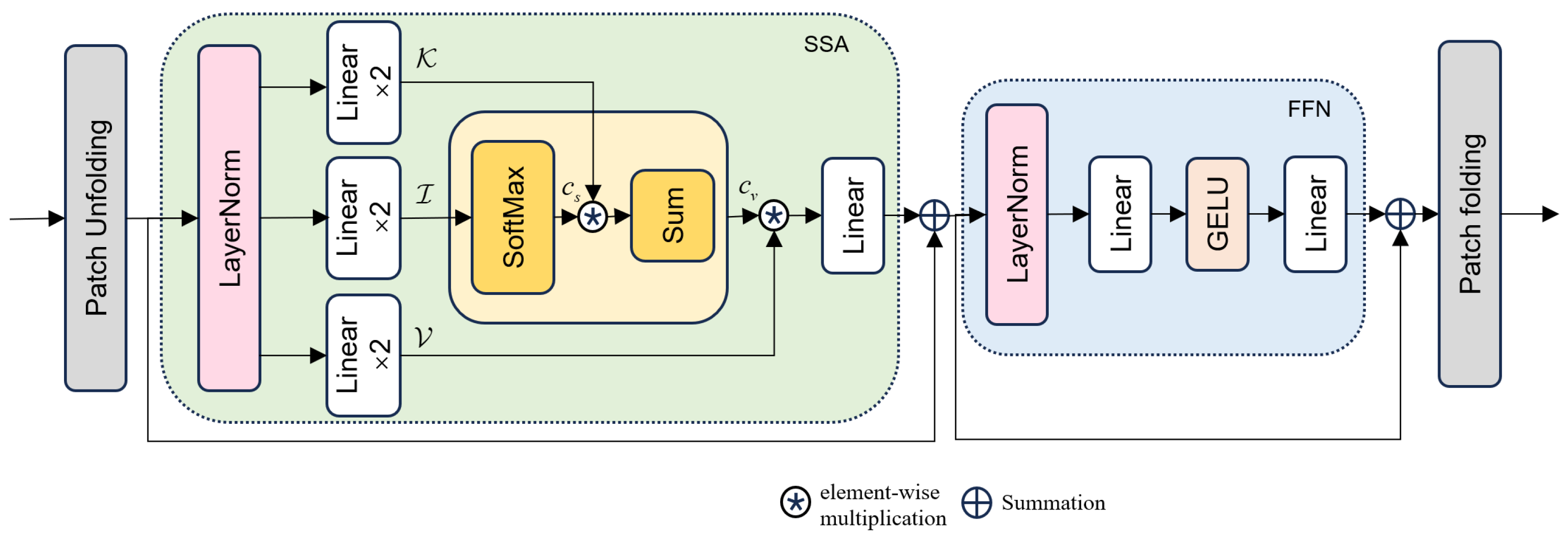
3.1.3. Mobilevitv3 Module

We introduce the Mobilevitv3 to enhance the feature representation of the image. The module comprises local block, global block and fusion block. The local block functions as a pre-processing stage to extract the local representation, and is composed of a depth-wise separable convolutional layer and a point-wise convolutional layer. The global block performs as a central unit through multiple Linear transformers learning the long-range dependence between pixels as well as global representation and is composed of a stack of transformers based on separable self-attention, a linear mapping layer. The fusion block is a linear mapping layer composed of a convolutional operation with a kernel size of $1\times 1$. The input of the Mobilevitv3 module respective processes through the local representation block and global representation block. Subsequently, after non-linear activation, the features are passed through the fusion block to obtain the final feature information. The Mobilevitv3 model is shown in Figure 5. The self-attention mechanism in the Linear Transformer module differs from the traditional multi-head self-attention mechanism in Transformers. Instead, the module employs linear separable self-attention (SSA). This attention mechanism replaces scaled dot-product attention between tokens with element-wise product between tokens, reducing the computational complexity from quadratic in terms of the number of tokens to linear. The computational process of SSA can be seen in Figure 6.

Figure 5. The structure of mobilevitv3 model.

Figure 6. Calculation process of SSA.

First, the input tokens $f\in {\mathbb{R}}^{C\times P\times N}$, C means the size of channels, P shows the number of tokens and N expresses the dimension of each token, are normalized by layer normalization, where the standard deviation and mean of the features of each sample are separately normalized to 1 and 0. Then they are subjected to linear mapping and divided into three unequal branches: input: $I\in {\mathbb{R}}^{1\times P\times N}$, key: $K\in {\mathbb{R}}^{d\times P\times N}$, and value: $V\in {\mathbb{R}}^{d\times P\times N}$. The I branch is processed by a softmax operation to obtain content scores $c_s$, which are then element-wise multiplied by K. After summation, the content vector is obtained, which is element-wise multiplied by V. This result then undergoes another linear mapping and is output to the feedforward unit for nonlinear processing. The process can be depicted as:

$$\begin{array}{cc}\hfill c_s& =\mathrm{softmax}\left(I\right),\hfill \\ \hfill c_v& =\sum _{i=1}^d{c}_s\times K,\hfill \\ \hfill \mathrm{SSA}& =H_{linear}\left(c_v\right)\times V,\hfill \end{array}$$

(3)

where d is the number of channels of K and V, $H_{linear}$ represents the linear mapping layer, and × means element-wise product. The output of the SSA module is the final feature representation of the input tokens.

3.2. Runway Localization

After the hazing removal algorithm processes the image, the UFLD algorithm infers runway points on the image. Due to various factors, it is necessary to filter and fit these detection points to accurately determine the positions of the detected left and right runway lines in the three-dimensional coordinate system. Furthermore, during the process of localization the runway lines, we utilized pixel depth information, which we obtained through two methods. When the CUAV is at a considerable distance from the carrier, accurate depth values cannot be obtained from the depth camera. Considering that there is an angle between the CUAV’s heading direction and the normal vector of the sea surface, we can approximate the depth information to achieve coarse positioning of the runway lines. On the contrary, when the CUAV is closer to the carrier, the depth camera can accurately capture depth values, enabling precise positioning of the runway lines directly.

Firstly, the runway points extracted by UFLD can be seen in Figure 7. Due to the accuracy of the runway detection algorithm and the uncertainty of parameters when manually annotating runway lines in images, points inferred by the network may deviate from the extension direction of the runway lines. As illustrated in Figure 7, the first three-runway points on the right side exhibit significant errors. Therefore, in the process of localization runway lines, it is necessary to eliminate runway points that cause large errors. Handling this problem in three-dimensional space is complex, thus necessitating the mapping of the runway to a two-dimensional space. Additionally, since points on runway lines should have the same height value, arithmetic operations can be performed in the pixel coordinate system. We can initially employ the Random Sample Consensus (RANSAC) method in the pixel coordinate system to remove outliers, facilitating the subsequent line-localization step in the global coordinate system. The process can be described as follows: Assuming there are i points in total, based on the principle of RANSAC, we can randomly select k points to perform the least squares localization (LSF) of a line. We use the distance from each point to the line as the error term and set a minimum error range. We then count the number of points falling within this range. If the number of points meets the criteria, we can consider the weights of the line appropriate. Then, we update the minimum error and recalculate until the minimum error no longer decreases.

Figure 7. Runway points detection result.

Secondly, after removing outliers, we need to map each point to three-dimensional space to fit the position of the runway line in the global coordinate system, achieving runway detection and localization. Pondering the trajectory of a CUAV from the starting point to above the flight deck, we can simplify this process as illustrated in Figure 8. Assuming that at the initial time instance, the position of the CUAV is $p_{b_0}$ with the attitude $R_{b_0}$, and when flying above the flight deck, the CUAV detects a point on the runway line at pixel coordinates $p_{pi{x}_i}$. At the moment, the position of the CUAV going to $p_{b_1}$ with the attitude $R_{b_1}$, the coordinates of this point in the body coordinate system relative to the initial time instance $p_{g_i}$ can be written as:

$$\begin{array}{c}{p}_{ca{m}_i}=depth·{\left[\begin{array}{ccc}{f}_x& 0& c_x\\ 0& f_y& c_y\\ 0& 0& 1\end{array}\right]}^{-1}·p_{pi{x}_i},i=1,2,3,...\hfill \\ p_{bod{y}_i}=R_c^b·p_c+p_b^c,\hfill \\ p_{g_i}=R_{b_1}·{\left(R_{b_0}\right)}^{-1}·p_b+p_{b_1}-p_{b_0}.\hfill \end{array}$$

(4)

Figure 8. Simulation of carrier-based unmanned aerial vehicle landing task process in our simulated environment.

$p_{ca{m}_i}$ denotes the coordinates of pixel point $p_{pi{x}_i}$ in the camera coordinate system, where i represents any point on the runway line, and $p_{bod{y}_i}$ represents the coordinates of this point in the body coordinate system. Additionally, $f_x,f_y,c_x,c_y$ is the camera intrinsic parameters, $R_c^b$ and $p_b^c$ are the rotation matrix and translation matrix of the camera coordinate system relative to the body coordinate system, respectively. The above process is repeated for each point on the runway line to obtain the global coordinates of the runway line in the global coordinate system. Assuming the line equation is $f(x_1,x_2,x_3)=w_0+w_1{x}_1+w_2{x}_2+w_3{x}_3$ and total pick out k points, the localization runway line equation can be expressed as:

$$\begin{array}{c}{w}^T=(w_0,w_1,w_2,w_3),\hfill \\ x=(1,x_1,x_2,x_3),\hfill \\ \mathcal{L}(w,x)=\sum _{i=1}^k{(y_i-w^T{x}^i)}^2.\hfill \end{array}$$

(5)

Our purpose is to minimize the loss function $\mathcal{L}(w,x)$ since we can employ the method of stochastic gradient descent to obtain the weight coefficients that minimize the loss function:

$$\begin{array}{c}\hfill w_t=w_{t-1}-\eta \frac{\partial \mathcal{L}}{\partial w},\end{array}$$

(6)

where $\eta$ is the step size, $w_t$ is the weight coefficient at step t, and $w_{t-1}$ is the weight coefficient at step $t-1$. The process is repeated until the loss function converges to a minimum value.

Finally, after performing the above steps, we can obtain the equations of the accurate straight lines for the left ($f_l(x_l,y_l,z_l)=w_l^0+w_l^1{x}_l+w_l^2{y}_l+w_l^3{z}_l$) and right ($f_r(x_r,y_r,z_r)=w_r^0+w_r^1{x}_r+w_r^2{y}_r+w_r^3{z}_r$) runway. The runway lines should be parallel ($w_l^0=w_r^0,w_l^1=w_r^1,w_l^2=w_r^2,w_l^3=w_r^3$). Therefore, the equation of the estimated central axis line can be expressed as $f_c(x_c,y_c,z_c)=(w_r^0+w_l^0)2+w_r^1{x}_c+w_r^2{y}_c+w_r^3{z}_c$. Hence, for the CUAV to align with the central axis of the runway, it is necessary to control the CUAV’s forward normal vector to align with the direction of the central axis line, while the CUAV’s center of mass should be as close as possible to the equation of the central axis line.

3.3. Dataset

The dataset was generated by Airsim (ver.1.8.1) [33], an open-source cross-platform simulator developed based on the Unreal Engine (ver.4.27). The excellent visual rendering power of Unreal Engine enables the simulator to produce high-quality visual simulation effects, making it suitable for a wide range of applications or research areas related to machine learning and artificial intelligence, such as deep learning, computer vision and automated visual data collection. The overall simulation utilizes the aircraft carrier Ronald Reagan (CVN-76) and the shipboard fighter J-15 to construct a landing scenario within an ocean environment. The carrier-based fighter took off from the deck of the aircraft carrier, flew to a distance of about 10 km from the carrier to enter the holding track, and then began to return, entering the landing track at a distance of about 5 km from the carrier, lowering its altitude to 300 m, lowering its altitude to 60 m at a distance of 800 m from the carrier, and finally gliding down to land on the carrier’s runway. Throughout the landing process, the center of the camera was always pointed at the runway on the deck of the carrier from the moment the aircraft entered the landing pattern. The ground truth of the trajectory was recorded by Airsim.

First, the geometric model of camera imaging needs to be established, that is, to obtain the camera’s internal parameter matrix K. The internal parameter matrix K can be expressed approximately as:

$$K=\left[\begin{array}{ccc}f/s& 0& w/2\\ 0& f/s& h/2\\ 0& 0& 0\end{array}\right]$$

(7)

where f represents the focal length, s represents the pixel size, and w and h represent the resolution of the image.

The camera in AirSim uses a perspective projection, then the focal length f and the pixel size s can be expressed as:

$$\begin{array}{cc}\hfill f& =\frac{1}{tan(fov/2)}\hfill \\ \hfill s& =\frac{2}{w}\hfill \end{array}$$

(8)

Consequently, in the AirSim simulation, the internal parameter matrix K of the camera can be expressed as:

$$K=\left[\begin{array}{ccc}\frac{w}{2tan(fov/2)}& 0& w/2\\ 0& \frac{w}{2tan(fov/2)}& h/2\\ 0& 0& 0\end{array}\right]$$

(9)

The parameters of the camera geometric model obtained through setup and computation, such as the camera internal reference matrix K, distortion sparse and field of view are summarised in Table 3.

Table 3. Parameters of camera model.

Parameters	Value
Intrinsic parameters	$\left[\begin{array}{ccc}732.35461496& 0& 640\\ 0& 732.35461496& 360\\ 0& 0& 1\end{array}\right]$
Radial distortion	$\left[\begin{array}{ccc}0& 0& 0\end{array}\right]$
Tangential distortion	$\left[\begin{array}{cc}0& 0\end{array}\right]$
FOV	70°
Resolution	1280 × 720

Next, the attitude change from the camera coordinate frame to the world coordinate frame still needs to be solved, that is, solving for the camera’s external parameter. We set a point directly in front of the deck of Ronald Reagan (CVN-76) as the origin of the world coordinate frame, and using the North-East-Down (NED) coordinate frame and right-handedness, the carrier’s coordinates in the world coordinate frame are (−148.45, 47.2, 31.26). The body coordinate frame uses the Forward Right Down (FRD) coordinate frame and right-handedness, which means that the airplane body is forward as the x-axis, perpendicular to the x-axis to the right as the y-axis direction, and perpendicular to the x-axis and y-axis downward as the z-axis, as shown in the Figure 9, which are the side view, front view, and top view in sequence. As shown in the Figure 10, the area surrounded by the red line is defined as the runway area.

Figure 9. Definition of body coordinate and three views of the J-15. (a) The side view of J-15. (b) The front view of J-15. (c) The top view of J-15.

Figure 10. Runway area of Ronald Reagan.

The final dataset acquired in the Airsim simulation consisted of a visible image with a depth map at the exact same camera position, using Airsim’s recording feature to continuously acquire the image and ground truth values.

4. Experiment Results and Discussions

In this section, to validate the optimization effect of our algorithm for the challenging task of carrier-based unmanned aerial vehicles landing on a ship deck in hazing conditions, we conducted numerous experiments in a simulated maritime environment. We separately verified the dehazing effect of the proposed algorithm in simulated hazeing maritime environments and evaluated the performance of runway detection and adjustment before and after dehazing, quantifying the errors.

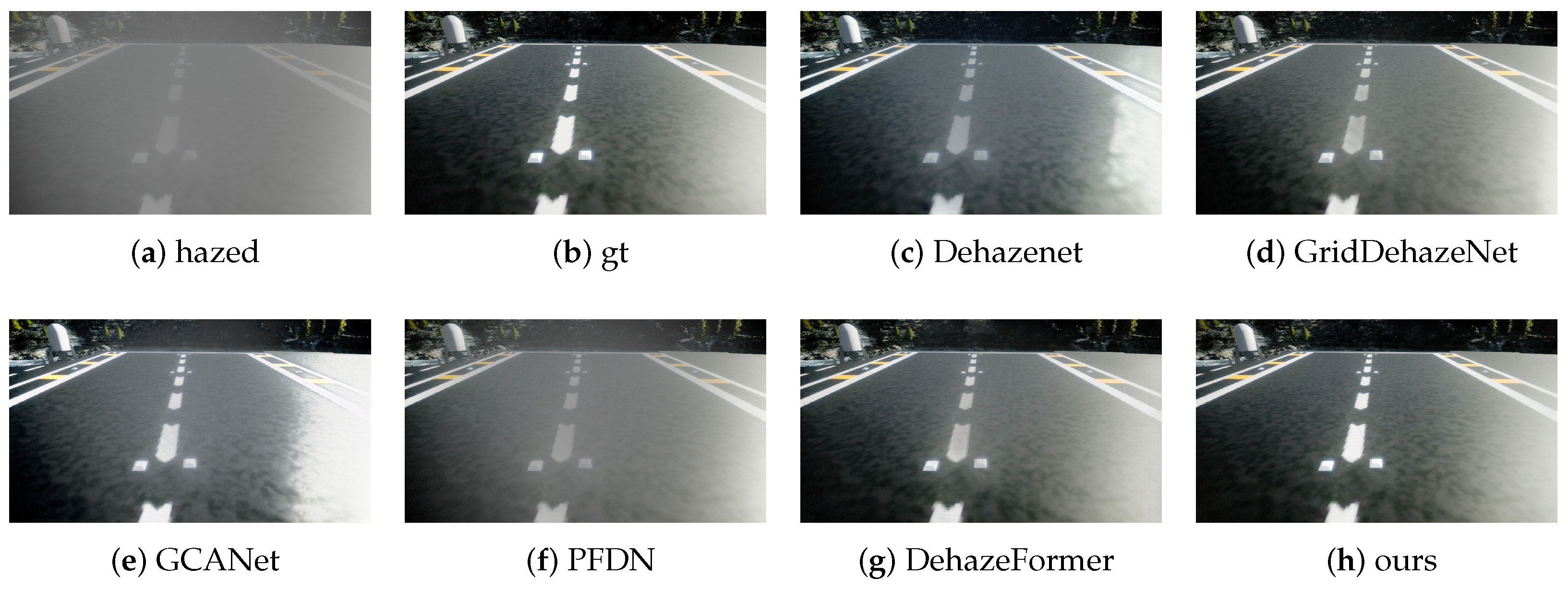
4.1. Dehazing Experiment

In this part, we first introduce the parameter settings and data preparation for the dehazing experiment. Then, we present the performance evaluation metrics and results of the dehazing experiment.

4.1.1. Parameter Settings

To accelerate the training speed of the model and obtain better generalization performance, we use the AdamW optimizer to train the model. The optimizer parameters ${\beta }_1=0.9$ and ${\beta }_2=0.999$ are set using the currently popular parameter settings. Considering the high total number of iterations used in our training, we set the weight decay parameter of the optimizer to $4\times {10}^{-3}$. The initial learning rate is set to $5\times {10}^{-4}$, and the learning rate is reduced by cosine annealing strategy gradually descending to $1\times {10}^{-7}$ within 600 K iterations. The batch size is set to 16 and the input image size is split to $512\times 512$. The loss function is the Peak Signal to Noise Ratio loss(PSNRLoss) [34] function. The training process is conducted on a single NVIDIA RTX 4090 GPU with a 13th Gen Intel(R) Core(TM) i9-13900KF CPU. The network framework is implemented using PyTorch 1.11.0, CUDA 11.3 and CUDNN 8.6.2.

In the simulation environment, to obtain the dataset for training the model, we control the CUAV to fly near the deck position and capture 600 pairs of clear and hazy images using the onboard camera. Among these, we selected 421 pairs as the training set and the remaining 179 pairs as the test set. Each image in the dataset has a size of $1280\times 720$ pixels. To reduce GPU memory consumption during training, we divided each image into eight equally sized sub-images of $512\times 512$ pixels, with overlapping regions between adjacent sub-images. Through this operation, the number of image pairs in both the training and test sets is increased to 3368 and 1512 pairs, respectively. Additionally, we employed image augmentation techniques such as horizontal flipping and vertical symmetry to enhance the diversity of the dataset and improve the generalization ability of the trained model. The metrics including Peak Signal to Noise Ratio (PSNR), Structural Similarity (SSIM) [35], and loss functions during the training process are shown in Figure 11a, Figure 11b and Figure 11c, respectively.

Figure 11. Reference values of various metrics during dehazing model training.

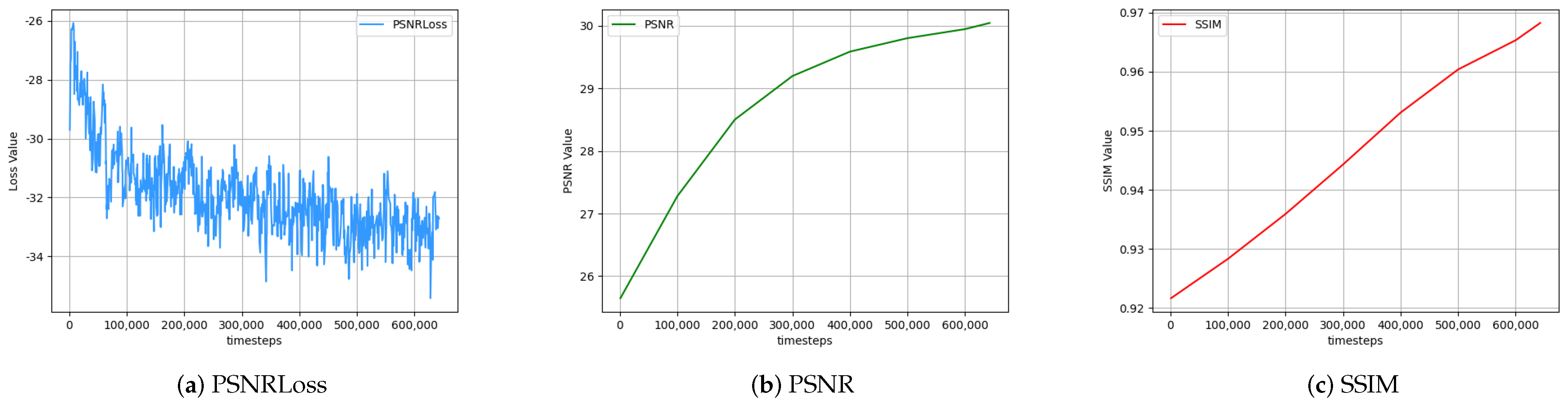
4.1.2. Performance Evaluation

The evaluation metrics applied in the dehazing experiment adopt PSNR and SSIM Index. The PSNR metric, which can quantify the reconstruction quality of the restored image, is based on the Mean Squares Error (MSE) between the ground truth image y and the restored image x. For an 8-bit RGB image, the formula for PSNR is as follows:

$$\begin{array}{c}MSE(x,y)=\frac{1}{H\times W}\sum _{i=1}^H\sum _{j=1}^W{∥y_{i,j}-x_{i,j}∥}_2^2,\hfill \\ PSNR=10·{log}_{10}\left(\frac{{255}^2}{MSE(x,y)}\right),\hfill \end{array}$$

(10)

where H and W are the height and width of the image, $y_{i,j}$ and $x_{i,j}$ are the pixel values of the ground truth image and the restored image. On the flip side, the SSIM metric can approximate the luminance, contrast and structure of the restored image compared to the ground truth image. The formula for SSIM is as follows:

$$SSIM(x,y)=\frac{(2{\mu }_x{\mu }_y+C_1)(2{\sigma }_{xy}+C_2)}{({\mu }_x^2+{\mu }_y^2+C_1)({\sigma }_x^2+{\sigma }_y^2+C_2)}.$$

(11)

where ${\mu }_x,{\mu }_y$ are the mean values of the restored image and the ground truth image, ${\sigma }_x^2,{\sigma }_y^2$ are the variances of the restored image and the ground truth image, ${\sigma }_{xy}$ is the covariance of the restored image and the ground truth image, $C_1$ and $C_2$ are constants to stabilize the division with weak denominator. In addition to the PSNRLoss, it can be calculated as:

$$PSNRLoss=-PSNR(x,y).$$

(12)

To evaluate the dehazing performance of our algorithm, we compared it with five other state-of-the-art (SOTA) algorithms based on four quantitative metrics: PSNR, SSIM, model parameters, and multiply-accumulate operations (MACs). The quantitative evaluation comparison is shown in Table 4.

Table 4. Comparison of various models on dehazing performance metrics, model parameters, memory consumption and latency.

Methods	PSNR	SSIM	Param (M)	MACs (G)	Latency-512 × 512 (ms)
hazed	13.98	0.635	-	-	-
DehazeNet [20]	20.15	0.863	0.009	0.581	1.34
GridDehazeNet [36]	26.26	0.948	0.956	21.49	12.65
GCANet [37]	24.33	0.921	0.702	18.41	3.69
PFDN [38]	28.97	0.961	11.27	50.20	7.31
DehazeFormer [10]	29.11	0.963	0.686	6.66	11.24
ours	30.18	0.972	0.484	4.91	8.63

In Table 4 of the quantitative metrics, our model achieved the best image quality indicators and minimized model parameters and memory consumption. Specifically, our model achieved a PSNR of 30.18 dB and an SSIM of 0.972, comparing DehazeFormer [10] with reducing $29.44\%$ #Param and $26.27\%$ memory computational cost as well as increasing 1.07 points in PSNR. The qualitative comparison of the dehazing effect is shown in Figure 12 and Figure 13. The results show that our model can effectively remove the haze in the image and restore the clear image, with the best visual effect among the six algorithms.

Figure 12. Visual comparison of dehazing effects of different models on sequence 1.

Figure 13. Visual comparison of dehazing effects of different models on sequence 2.

In addition, we conduct ablation experiments to verify the effectiveness of the network modules used in this study and the impact of the image augmentation methods used during training on the training metrics of the network model. In the ablation experiment, we replaced the MixAttention and the Mobilevitv3 module used in this paper with conventional depthwise separable convolutions and the transformer module used in [10], respectively, while also using no image segmentation and image augmentation operations on the dataset as the baseline. The result is shown in Table 5.

Table 5. Results of ablation experiments.

Baseline	MixAttention↑	Mobilevitv3↑	Data Augmentation↑	PSNR	SSIM
√	×	×	√	29.02	0.962
√	√	×	√	29.54	0.967
√	√	√	√	30.18	0.972
√	√	√	×	30.10	0.969

According to the ablation experiment result of Table 5, after replacing conventional depthwise separable convolutions with the MixAttention module, the PSNR increased by 0.52 dB. Subsequently, replacing the transformer module with the Mobilevitv3 used in this paper led to a further increase in PSNR by 0.64 dB. Finally, applying data augmentation to the dataset resulted in a PSNR improvement of 0.08 dB. The ablation experiment results demonstrate the effectiveness of the network modules used in this paper and the impact of the image augmentation method on the training metrics of the network model.

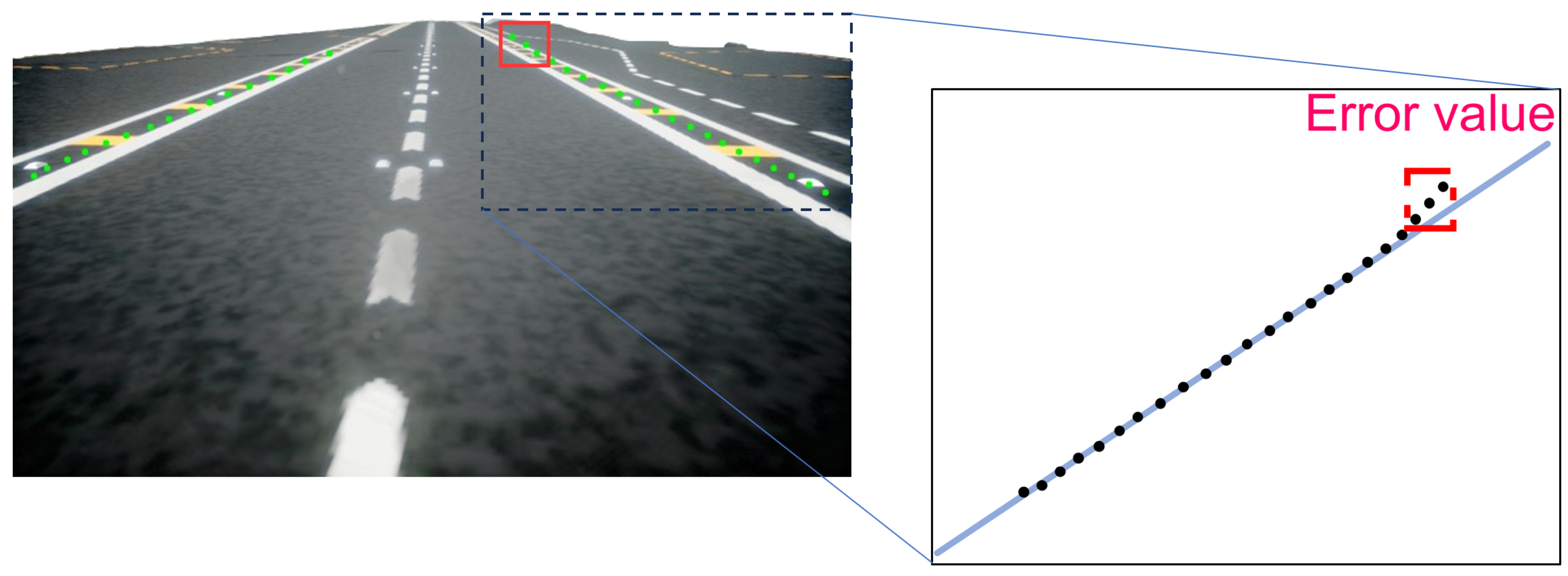
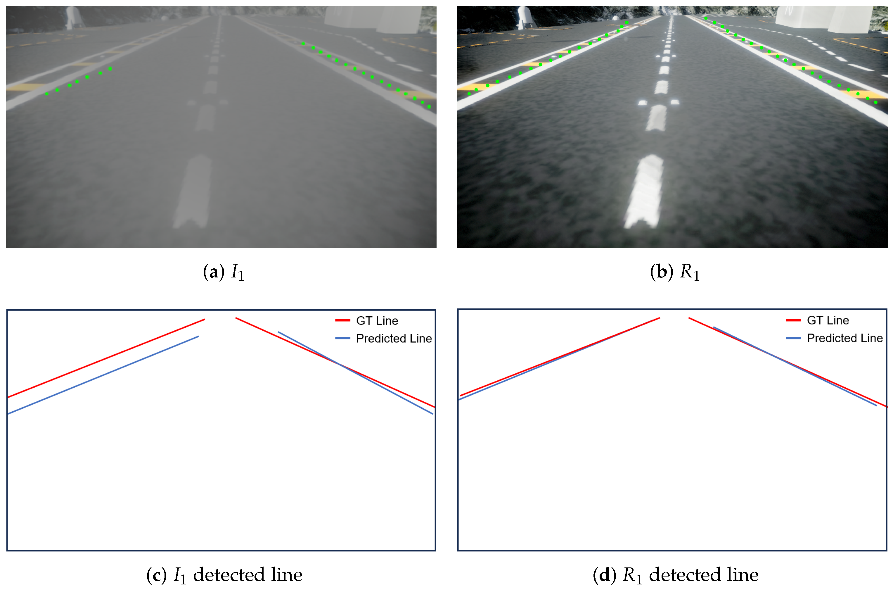
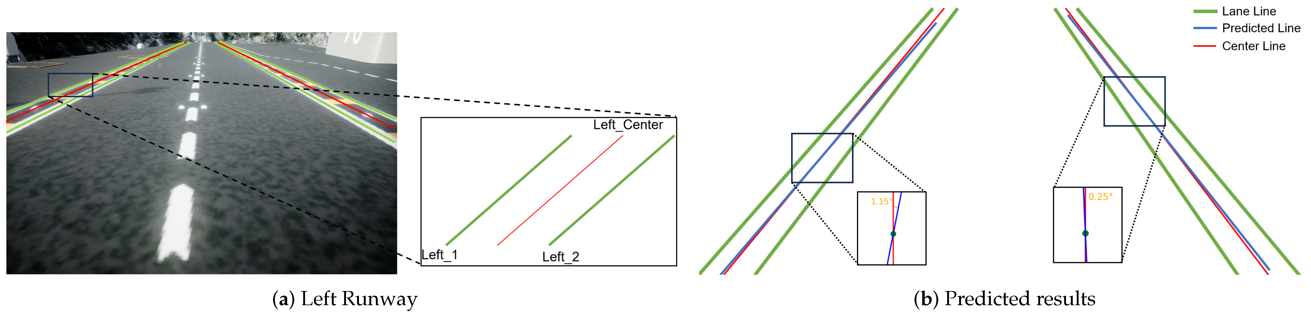
4.2. Runway Localization Analysis

In this part, we primarily elaborate on two aspects. Firstly, we compare and analyze the runway detection performance before and after dehazing. Subsequently, we quantify the errors of the localization equations for the left and right runway lines.

4.2.1. Dehazed Function

To demonstrate the necessity of image dehazing, we selected two hazed images as the input images and observed the runway detection performance before and after dehazing. The results are shown in Figure 14. From Figure 14, we can observe that in a hazed image $I_1$ compared to the dehazed images $R_1$, the UFLD algorithm detects fewer points in the hazed images, and the extension directions of these points deviate significantly from the direction of the ground truth (GT) runway lines. These two defects could lead to large errors in the localization runway line equations, which are undoubtedly fatal for the landing process of the CUAV. This is mainly attributed to the fact that in hazed images, the average pixel value of the image rises while the variance is reduced due to the degradation of the image. As a result, some of the edge information in the image is lost, and the detection algorithm cannot effectively detect the edges of the runway lines, leading to a decrease in detection performance. Dehazing operations mitigate this phenomenon, thereby enhancing the performance of runway line detection algorithms.

Figure 14. Results of runway detection algorithms before and after dehazing.

4.2.2. Localization Details

Indeed, taking the left runway line as an example (e.g., Figure 15a), each runway line consists of two white lines and several yellow lines intersecting with the white lines. For clarity of representation, we simplify the two white lines as two green lines and depict the centerline using a red line. The predicted runway is painted by the blue line.

Figure 15. The predicted result by UFLD.

In Figure 15b, we utilize the UFLD algorithm to detect the centerline of the left and right runway. Considering that the deck of aircraft carriers and similar vessels is a flat surface, the height values of the detected points should be close to each other. Based on this, we reduce the multidimensional linear regression problem to a two-dimensional information regression problem. Hence, the predicted centerline can be written to:

$$f(x,y,z)=w_0+w_{1}x+w_{2}y, z=w_3=height.$$

(13)

where $w_0,w_1,w_2$ are the weight coefficients of the centerline equation. $z=w_3=height$ is the height value of the detected point. Consequently, slope $k=\frac{w_1}{w_2}$ and intercept $b=\frac{w_0}{w_2}$ can be calculated.

To quantify the impact of dehazing on runway detection accuracy, we used the UFLD algorithm as the baseline and compared it with two other conventional runway line detection algorithms. We conducted ten experiments in total, calculating the average slope k, intercept b, and height h of the localization lines. The angle difference $\Delta \theta$ and intercept difference $\Delta b$ between the localization runway lines and the ground truth runway lines are used as evaluation metrics. The experimental results are shown in Table 6.

Table 6. Comparison of localization results for each algorithm’s performance.

Method	Direction	k	b	h	$\Delta \theta$	$\left|\Delta b\right|$
UFLD [5]	Left	−0.01243	45.047335	6.0641224	8.5456°	9.258812
	Right	−0.085547	26.223431	6.0570601	3.9949°	5.333762
Lanedet [39]	Left	−0.292449	22.275809	6.0754075	7.0437°	13.51271
	Right	−0.066909	30.247141	6.0607728	5.0566°	9.357472
SAD [40]	Left	−0.269742	26.614948	6.0958085	5.8380°	9.173575
	Right	−0.107914	25.097884	6.0965721	2.7254°	4.208215
ours (UFLD + dehazed)	Left	−0.139172	37.652321	6.0611483	1.3347°	1.863798
	Right	−0.15732	20.937649	6.0613821	0.0559°	0.047980

After our calculations in the simulation environment, the actual equations for the centerlines of the left and right runway should be:

$$\begin{array}{c}{f}_{left}(x,y)=0.16300x+y-35.788523, z=6.0800000,\hfill \\ f_{right}(x,y,z)=0.15632x+y-20.889669, z=6.0800000.\hfill \end{array}$$

(14)

From Table 6, it can be seen that the four listed methods show little error in the height direction compared to the ground truth, but the slope and intercept values show significant differences for the UFLD [5], Lanedet [39], and SAD [40] algorithms. For example, the slope and intercept of the left runway line localization by the UFLD algorithm are 0.15 and 9.25 m less than the ground truth, respectively, with an angle difference of 8.5456° between the localization and ground truth left runway lines. The slope and intercept of the right runway line localization by the UFLD algorithm are approximately 0.07 and 5.33 m less than the ground truth, respectively, with an angle difference of 3.9949° between the localization and ground truth right runway lines. After enhancement by our algorithm, the differences between the slope and intercept of the left runway line and the ground truth were reduced to 0.02489 and 1.85 m, respectively, with the angle difference reduced to 1.3347°. For the right runway line, the differences between the slope and intercept and the ground truth were reduced to 0.00122 and 0.051 m, respectively, with the angle difference reduced to 0.0559°. It can be observed that the runway detection accuracy after dehazing has improved by approximately 86%. In summary, our entire algorithm pipeline can effectively improve the landing accuracy of CUAVs under hazed conditions, thus enhancing the safety of the landing process.

5. Conclusions

In this paper, to address the issue of reduced accuracy of onboard sensors of CUAVs due to hazing weather conditions, leading to unreliable and unsafe execution of landing tasks, we propose a dehazing algorithm and a runway detection and localization algorithm to tackle the aforementioned problem.

In the dehazing network model, we propose a U-shaped network structure, introduce the lightweight fused attention mechanism module combining simple spatial attention and simple channel attention and utilize a Transformer module with linear computational complexity. This implementation ensures both enhanced dehazing capability of the network and low computational cost during forward propagation. Considering real-time requirements, we select the UFLD algorithm as the runway detection algorithm. By filtering and localization the detected points, we can obtain highly accurate localization runway line equations.

Finally, we conducted extensive experiments on our entire algorithm framework. We compared the performance of our dehazing model with other state-of-the-art models, as well as the localization results obtained from our dehazing algorithm and localization method. The experiments demonstrate that our dehazing algorithm achieves the best dehazing effect while significantly improving runway detection performance under hazed conditions.

Additionally, to further ensure the safe and reliable landing of carrier-based UAVs, it is important to note the following: First, our image dehazing model may not address other types of image degradation, such as rainy images or motion-blurred images. Second, due to the limitations of the dataset used for training, the optimization effect on images in heavy fog conditions may not be satisfactory. Third, this paper does not address the control decision methods for carrier-based UAVs after detecting the runway lines. Our future work will focus on designing better algorithms to address these issues.

References

1. Ma, N.; Weng, X.; Cao, Y.; Wu, L. Monocular-Vision-Based Precise Runway Detection Applied to State Estimation for Carrier-Based UAV Landing. Sensors 2022, 22, 8385. [Google Scholar] [CrossRef] [PubMed]
2. Wang, Y.; Teoh, E.K.; Shen, D. Lane detection and tracking using B-Snake. Image Vis. Comput. 2004, 22, 269–280. [Google Scholar] [CrossRef]
3. Aly, M. Real time detection of lane markers in urban streets. In Proceedings of the 2008 IEEE Intelligent Vehicles Symposium, Eindhoven, The Netherlands, 4–6 June 2008; IEEE: Piscataway, NJ, USA, 2008; pp. 7–12. [Google Scholar]
4. Pan, X.; Shi, J.; Luo, P.; Wang, X.; Tang, X. Spatial as deep: Spatial cnn for traffic scene understanding. In Proceedings of the AAAI Conference on Artificial Intelligence, New Orleans, LA, USA, 2–7 February 2018; Volume 32. [Google Scholar]
5. Qin, Z.; Wang, H.; Li, X. Ultra fast structure-aware deep lane detection. In Proceedings of the Computer Vision—ECCV 2020: 16th European Conference, Glasgow, UK, 23–28 August 2020; Part XXIV 16. Springer: Berlin/Heidelberg, Germany, 2020; pp. 276–291. [Google Scholar]
6. Gurghian, A.; Koduri, T.; Bailur, S.V.; Carey, K.J.; Murali, V.N. Deeplanes: End-to-end lane position estimation using deep neural networksa. In Proceedings of the IEEE Conference on Computer Vision and Pattern Recognition Workshops, Las Vegas, NV, USA, 26 June–1 July 2016; pp. 38–45. [Google Scholar]
7. Huval, B.; Wang, T.; Tandon, S.; Kiske, J.; Song, W.; Pazhayampallil, J.; Andriluka, M.; Rajpurkar, P.; Migimatsu, T.; Cheng-Yue, R.; et al. An empirical evaluation of deep learning on highway driving. arXiv 2015, arXiv:1504.01716. [Google Scholar]
8. Lee, S.; Kim, J.; Shin Yoon, J.; Shin, S.; Bailo, O.; Kim, N.; Lee, T.H.; Seok Hong, H.; Han, S.H.; So Kweon, I. Vpgnet: Vanishing point guided network for lane and road marking detection and recognition. In Proceedings of the IEEE International Conference on Computer Vision, Venice, Italy, 22–29 October 2017; pp. 1947–1955. [Google Scholar]
9. Huang, Y.; Chen, S.; Chen, Y.; Jian, Z.; Zheng, N. Spatial-temproal based lane detection using deep learning. In Proceedings of the Artificial Intelligence Applications and Innovations: 14th IFIP WG 12.5 International Conference, AIAI 2018, Rhodes, Greece, 25–27 May 2018; Proceedings 14. Springer: Berlin/Heidelberg, Germany, 2018; pp. 143–154. [Google Scholar]
10. Song, Y.; He, Z.; Qian, H.; Du, X. Vision transformers for single image dehazing. IEEE Trans. Image Process. 2023, 32, 1927–1941. [Google Scholar] [CrossRef] [PubMed]
11. Lu, L.; Xiong, Q.; Chu, D.; Xu, B. MixDehazeNet: Mix Structure Block For Image Dehazing Network. arXiv 2023, arXiv:2305.17654. [Google Scholar]
12. Gui, J.; Cong, X.; Cao, Y.; Ren, W.; Zhang, J.; Zhang, J.; Cao, J.; Tao, D. A comprehensive survey and taxonomy on single image dehazing based on deep learning. ACM Comput. Surv. 2023, 55, 1–37. [Google Scholar] [CrossRef]
13. McCartney, E.J. Optics of the Atmosphere: Scattering by Molecules and Particles; John Wiley and Sons, Inc.: New York, NY, USA, 1976. [Google Scholar]
14. Narasimhan, S.G.; Nayar, S.K. Contrast restoration of weather degraded images. IEEE Trans. Pattern Anal. Mach. Intell. 2003, 25, 713–724. [Google Scholar] [CrossRef]
15. Nayar, S.K.; Narasimhan, S.G. Vision in bad weather. In Proceedings of the Seventh IEEE International Conference on Computer Vision, Kerkyra, Greece, 20–27 September 1999; IEEE: Piscataway, NJ, USA, 1999; Volume 2, pp. 820–827. [Google Scholar]
16. He, K.; Sun, J.; Tang, X. Single image haze removal using dark channel prior. IEEE Trans. Pattern Anal. Mach. Intell. 2010, 33, 2341–2353. [Google Scholar] [PubMed]
17. Fattal, R. Dehazing using color-lines. Acm Trans. Graph. (TOG) 2014, 34, 1–14. [Google Scholar] [CrossRef]
18. Liu, J.; Liu, W.; Sun, J.; Zeng, T. Rank-one prior: Toward real-time scene recovery. In Proceedings of the IEEE/CVF Conference on Computer Vision and Pattern Recognition, Nashville, TN, USA, 20–25 June 2021; pp. 14802–14810. [Google Scholar]
19. Zhu, Q.; Mai, J.; Shao, L. A fast single image haze removal algorithm using color attenuation prior. IEEE Trans. Image Process. 2015, 24, 3522–3533. [Google Scholar] [PubMed]
20. Cai, B.; Xu, X.; Jia, K.; Qing, C.; Tao, D. Dehazenet: An end-to-end system for single image haze removal. IEEE Trans. Image Process. 2016, 25, 5187–5198. [Google Scholar] [CrossRef] [PubMed]
21. Zhang, H.; Patel, V.M. Densely connected pyramid dehazing network. In Proceedings of the IEEE Conference on Computer Vision and Pattern Recognition, Salt Lake City, UT, USA, 18–23 June 2018; pp. 3194–3203. [Google Scholar]
22. Li, B.; Peng, X.; Wang, Z.; Xu, J.; Feng, D. Aod-net: All-in-one dehazing network. In Proceedings of the IEEE International Conference on Computer Vision, Venice, Italy, 22–29 October 2017; pp. 4770–4778. [Google Scholar]
23. Ren, W.; Ma, L.; Zhang, J.; Pan, J.; Cao, X.; Liu, W.; Yang, M.H. Gated fusion network for single image dehazing. In Proceedings of the IEEE Conference on Computer Vision and Pattern Recognition, Salt Lake City, UT, USA, 18–23 June 2018; pp. 3253–3261. [Google Scholar]
24. Guo, C.L.; Yan, Q.; Anwar, S.; Cong, R.; Ren, W.; Li, C. Image dehazing transformer with transmission-aware 3d position embedding. In Proceedings of the IEEE/CVF Conference on Computer Vision and Pattern Recognition, New Orleans, LA, USA, 18–24 June 2022; pp. 5812–5820. [Google Scholar]
25. Chen, H.; Wang, Y.; Guo, T.; Xu, C.; Deng, Y.; Liu, Z.; Ma, S.; Xu, C.; Xu, C.; Gao, W. Pre-trained image processing transformer. In Proceedings of the IEEE/CVF Conference on Computer Vision and Pattern Recognition, Nashville, TN, USA, 20–25 June 2021; pp. 12299–12310. [Google Scholar]
26. Liu, Z.; Lin, Y.; Cao, Y.; Hu, H.; Wei, Y.; Zhang, Z.; Lin, S.; Guo, B. Swin transformer: Hierarchical vision transformer using shifted windows. In Proceedings of the IEEE/CVF International Conference on Computer Vision, Nashville, TN, USA, 20–25 June 2021; pp. 10012–10022. [Google Scholar]
27. Tang, J.; Li, S.; Liu, P. A review of lane detection methods based on deep learning. Pattern Recognit. 2021, 111, 107623. [Google Scholar] [CrossRef]
28. Chougule, S.; Koznek, N.; Ismail, A.; Adam, G.; Narayan, V.; Schulze, M. Reliable multilane detection and classification by utilizing CNN as a regression network. In Proceedings of the European Conference on Computer Vision (ECCV) Workshops, Munich, Germany, 8–14 September 2018; pp. 740–752. [Google Scholar]
29. Chiu, K.Y.; Lin, S.F. Lane detection using color-based segmentation. In Proceedings of the IEEE Proceedings. Intelligent Vehicles Symposium, Las Vegas, NV, USA, 6–8 June 2005; IEEE: Piscataway, NJ, USA, 2005; pp. 706–711. [Google Scholar]
30. Zheng, T.; Fang, H.; Zhang, Y.; Tang, W.; Yang, Z.; Liu, H.; Cai, D. Resa: Recurrent feature-shift aggregator for lane detection. In Proceedings of the AAAI Conference on Artificial Intelligence, Virtual, 2–9 February 2021; Volume 35, pp. 3547–3554. [Google Scholar]
31. Zheng, T.; Huang, Y.; Liu, Y.; Tang, W.; Yang, Z.; Cai, D.; He, X. Clrnet: Cross layer refinement network for lane detection. In Proceedings of the IEEE/CVF Conference on Computer Vision and Pattern Recognition, New Orleans, LA, USA, 18–24 June 2022; pp. 898–907. [Google Scholar]
32. Han, J.; Deng, X.; Cai, X.; Yang, Z.; Xu, H.; Xu, C.; Liang, X. Laneformer: Object-aware row-column transformers for lane detection. In Proceedings of the AAAI Conference on Artificial Intelligence; 2022; Volume 36, pp. 799–807. [Google Scholar]
33. Shah, S.; Dey, D.; Lovett, C.; Kapoor, A. AirSim: High-Fidelity Visual and Physical Simulation for Autonomous Vehicles. arXiv 2017, arXiv:1705.05065. [Google Scholar] [CrossRef]
34. Chen, L.; Lu, X.; Zhang, J.; Chu, X.; Chen, C. Hinet: Half instance normalization network for image restoration. In Proceedings of the IEEE/CVF Conference on Computer Vision and Pattern Recognition, Nashville, TN, USA, 19–25 June 2021; pp. 182–192. [Google Scholar]
35. Wang, Z.; Bovik, A.C.; Sheikh, H.R.; Simoncelli, E.P. Image quality assessment: From error visibility to structural similarity. IEEE Trans. Image Process. 2004, 13, 600–612. [Google Scholar] [CrossRef] [PubMed]
36. Liu, X.; Ma, Y.; Shi, Z.; Chen, J. Griddehazenet: Attention-based multi-scale network for image dehazing. In Proceedings of the IEEE/CVF International Conference on Computer Vision, Seoul, Repuiblic of Korea, 27 October–2 November 2019; pp. 7314–7323. [Google Scholar]
37. Chen, D.; He, M.; Fan, Q.; Liao, J.; Zhang, L.; Hou, D.; Yuan, L.; Hua, G. Gated context aggregation network for image dehazing and deraining. In Proceedings of the 2019 IEEE Winter Conference on Applications of Computer Vision (WACV), Waikoloa, HI, USA, 7–11 January 2019; IEEE: Piscataway, NJ, USA, 2019; pp. 1375–1383. [Google Scholar]
38. Dong, J.; Pan, J. Physics-based feature dehazing networks. In Proceedings of the Computer Vision—ECCV 2020: 16th European Conference, Glasgow, UK, 23–28 August 2020; Part XXX 16. Springer: Berlin/Heidelberg, Germany, 2020; pp. 188–204. [Google Scholar]
39. Neven, D.; De Brabandere, B.; Georgoulis, S.; Proesmans, M.; Van Gool, L. Towards end-to-end lane detection: An instance segmentation approach. In Proceedings of the 2018 IEEE Intelligent Vehicles Symposium (IV), Changshu, China, 26–30 June 2018; IEEE: Piscataway, NJ, USA, 2018; pp. 286–291. [Google Scholar]
40. Hou, Y.; Ma, Z.; Liu, C.; Loy, C.C. Learning lightweight lane detection cnns by self attention distillation. In Proceedings of the IEEE/CVF International Conference on Computer Vision, Seoul, Repuiblic of Korea, 27 October–2 November 2019; pp. 1013–1021. [Google Scholar]
Disclaimer/Publisher’s Note: The statements, opinions and data contained in all publications are solely those of the individual author(s) and contributor(s) and not of MDPI and/or the editor(s). MDPI and/or the editor(s) disclaim responsibility for any injury to people or property resulting from any ideas, methods, instructions or products referred to in the content.
Article Metrics
Citations
Article Access Statistics
Multiple requests from the same IP address are counted as one view.