Abstract
Tomatoes are a crop of significant economic importance, and disease during growth poses a substantial threat to yield and quality. In this paper, we propose IBSA_Net, a tomato leaf disease recognition network that employs transfer learning and small sample data, while introducing the Shuffle Attention mechanism to enhance feature representation. The model is optimized by employing the IBMax module to increase the receptive field and adding the HardSwish function to the ConvBN layer to improve stability and speed. To address the challenge of poor generalization of models trained on public datasets to real environment datasets, we developed an improved PlantDoc++ dataset and utilized transfer learning to pre-train the model on PDDA and PlantVillage datasets. The results indicate that after pre-training on the PDDA dataset, IBSA_Net achieved a test accuracy of 0.946 on a real environment dataset, with an average precision, recall, and F1-score of 0.942, 0.944, and 0.943, respectively. Additionally, the effectiveness of IBSA_Net in other crops is verified. This study provides a dependable and effective method for recognizing tomato leaf diseases in real agricultural production environments, with the potential for application in other crops.
1. Introduction
In agriculture, the identification of tomato leaf diseases has traditionally relied on manual identification, which can be subject to fluctuations in accuracy due to the variability in the experience and expertise of the human identifiers [1]. Additionally, the process is laborious and time-consuming, making it challenging to identify a large number of experts with sufficient experience in the identification of tomato leaf diseases [2].
Recent advances in machine learning and deep learning techniques have revolutionized crop pest and disease identification by enabling the automated detection of leaf diseases. However, traditional machine learning methods face limitations, such as the need for manual screening of features and the inability to perform fully automated disease identification, including disease classification [3,4,5,6]. Conventional convolutional networks are also not optimal for recognizing single diseases in crop disease identification and may not accurately identify diseased regions of the crop [7,8,9].
Annabel and Muthulakshmi addressed these limitations by employing the random forest (RF) algorithm to detect three different types of tomato leaf diseases, namely bacterial spots, tomato mosaic viruses, late blight, and healthy leaf disease. The algorithm achieved an impressive accuracy of 94.10%, surpassing the results obtained using the SVM and MDC algorithms, which recorded accuracies of 82.60% and 87.60%, respectively, when applied to the same dataset [10]. In a similar vein, Das et al. (2020) developed a system that could detect seven distinct types of tomato leaf diseases using SVM, logistic regression (LR), and RF. The Haralick algorithm was employed to extract the texture features of the leaves, and the classifiers were used to classify the extracted features. The results of the study revealed that SVM outperformed the other two algorithms, recording an accuracy of 87.60%, followed by RF and LR, which recorded accuracies of 70.05% and 67.30%, respectively [11].
Deep learning models have been widely applied in plant leaf disease detection and classification. Thangaraj et al., proposed a TL-DCNN model to identify tomato leaf diseases and compared the performance of Adam, RMSprop and SGD optimizers, finding that the modified-Xception model with Adam optimizer achieved the best results [12]. Pan Zhang et al., used seven pre-trained EfficientNet-B0-B7 models to train and test on four datasets of cucumber powdery mildew, downy mildew, healthy leaves and a combination of powdery mildew and downy mildew, finding that efficient-B4 achieved the highest accuracy (97%) for cucumber disease classification in four tasks [13]. Zhe Tang et al., proposed a lightweight convolutional neural network model to diagnose grape diseases, including black rot, black measles and leaf blight. The model incorporated the squeeze-and-excitation (SE) mechanism into ShuffleNet and achieved 99.14% accuracy on PlantVillage dataset [14]. Utpal Barman proposed an SSCNN network for citrus leaf disease classification, which can be deployed on smartphones and has higher accuracy and less computation time than MobileNet [15]. Victor Gonzalez-Huitron et al., used four typical convolutional network models trained on Plant Village to find the optimal model and present a user interface on Raspberry Pi [16]. Amreen Abbas et al., generated synthetic images of tomato leaves by constructing a C-GAN network for the network training [17]. Brahimi et al. (2017) used GoogLeNet and AlexNet models to detect tomato plant diseases and found that GoogLeNet had an accuracy of 99.18%, higher than AlexNet’s 98.60% [18]. Jiang et al. (2020) proposed an improved ResNet50 model to classify three different types of tomato leaf diseases (spot disease, yellow leaf curling and late blight), which used leaky ReLU activation function and modified the filter size in each convolutional layer to 11 × 11 to improve accuracy. The experimental results showed that ResNet50 achieved 98% accuracy on the test dataset [19]. Rubanga et al. (2020) used pre-trained CNN architectures (such as Inception V3, VGG16, VGG19 and ResNet) to detect tuta absoluta virus infection in tomato leaves, finding that Inception V3 had a detection accuracy of 87.20% better than other architectures [20].
Ullah, Z. used a hybrid deep learning approach to detect tomato plant diseases from leaf images, integrating pre-trained EfficientNetB3 and MobileNet models to achieve 99.92% accuracy [21]. Waheed, H. developed an Android system for diagnosing ginger plant diseases by training VGG and MobileNetV2 models on a real dataset of ginger leaf images, achieving real-time detection with high performance [22]. Ulutaş proposed two CNN models for tomato leaf disease detection, optimized via fine-tuning, particle swarm optimization, and grid search. Their ensemble model achieved 99.60% accuracy with fast training and testing times [23]. Luo, Y. created “LiteCNN,” a lightweight neural network that achieved 95.24% accuracy through knowledge distillation. The network was then deployed on an FPGA for a low-power, high-precision, and fast plant disease recognition terminal, suitable for real-time recognition in the field [24]. Fan, X. proposed a transfer learning-based deep feature descriptor that combined deep and hand-crafted features through feature fusion to capture local texture information in plant leaf images. The approach achieved accuracies of 99.79%, 92.59%, and 97.12% on three different datasets [25]. Janarthan, S. proposed a mobile lightweight deep learning model that achieved accuracies of 97%, 97.1%, and 96.4% on apple, citrus, and tomato leaf datasets, respectively. The model had approximately 88 million multiply-accumulate operations, 260,000 parameters, and 1 MB of storage space [26].
Image-based methods for tomato leaf disease recognition have limitations. They require large-scale annotated datasets for training, which are difficult to obtain and may lack representativeness. Additionally, they do not fully consider the diversity and complexity of image acquisition conditions in real environments, such as illumination, angle, occlusion, noise, and other factors. Transfer learning techniques are also not effectively utilized to improve the model’s generalization and adaptation abilities on different datasets. To overcome these limitations, this paper proposes a novel convolutional neural network model, IBSA_Net, which combines the inverted bottleneck structure and Shuffle Attention mechanism. The paper also explores the impact of activation functions, such HardSwish, and MaxPool layer, on the network’s performance. The proposed model achieves high accuracy, precision, recall, and F1-score on tomato leaf disease classification tasks and quickly identifies tomato leaf disease regions in real environments. Furthermore, this paper verifies the validity of IBSA_Net on other crops. The main contributions of this paper are as follows:
- The IBMax module is proposed to enhance model recognition accuracy by downsizing feature maps and expanding the perceptual field.
- The Shuffle Attention mechanism is introduced and alternately embedded into the network modules to enable the model to focus accurately on tomato leaf disease regions.
- The PlantDoc++ dataset is constructed, and an innovative transfer learning approach is utilized to address the problem of models trained on a single background dataset being unable to generalize to real-world agricultural production environments.
2. Materials and Methods
2.1. Data Set Structure
The three datasets used in this experiment are the tomato leaf disease dataset in Plant Village, the PlantVillage Dataset with Data Augmentation (PDDA) on the Kaggle data site, and the extended dataset based on the PlantDoc dataset, PlantDoc++ [27]. There are 39 different types of leaves in Plant Village, 10 of which belong to tomatoes. The tomato leaf disease dataset has nine disease images and one healthy leaf image. However, since the background of tomato leaves in Plant Village is relatively homogeneous, there may be a need to identify tomato leaf disease for complex backgrounds in real situations. The PlantVillage Dataset with Data Augmentation (PDDA), created from the PlantVillage dataset, was used to simulate tomato leaves photographed in a natural environment by fusing tomato leaves with a complex background. The PlantDoc dataset is a dataset of tomato leaf diseases taken in a natural environment, with eight types ranging from a few dozen to two hundred images per category. Since the original PlantDoc dataset has different disease categories than PlantVillage, it has unclear and watermarked images. Therefore, this paper expands PlantDoc by crawling relevant images on the web through ImageAssistant. After filtering and deleting, PlantDoc has the same disease categories as PlantVillage and ensures the clarity of each image. The modified dataset is called PlantDoc++.
In this paper, all models are trained on PlantVillage and PDDA, respectively, and the data set is divided using the ratio of training set: test set of 8:2. The number of the training set and test set are the same for PlantVillage and PDDA, Please refer to Table 1 for detailed information. After training on the two different datasets, some series of models trained on the corresponding datasets are called model clusters. The PlantVillage model cluster and PDDA model cluster are migrated to learn on the PlantDoc++ training set and finally tested on the PlantDoc++ test set, respectively. For PlantDoc++, the ratio of the training set to the test set is 5:5.

Table 1.
PlantVillage and PDDA dataset.
2.2. Data Pre-Processing
The data enhancement methods used include 30°, 45°, and 60° rotations of the samples; random cropping of the images using a 150 × 150 size crop frame, cropping and then scaling to the original size; the random flip of the images, and other operations.
3. IBSA_Net Model Construction and Module Composition
3.1. Introduce Inverted Bottleneck Structure to Improve Network Accuracy
The bottleneck structure was first proposed in the ResNet model [28]. That paper pointed out that the model’s training time and parameters can be reduced by changing the original structure of two convolutional layers with a convolutional kernel size of 3 × 3 to a structure with a 3 × 3 convolution between two 1 × 1 convolutions. The diagram of the convolutional structure before and after the improvement is shown as follows.
As shown in Figure 1, after the improvement, the number of input and output channels are both 256, while the number of input and output channels of the middle convolution is 64, and this is “thick at both ends and thin in the middle” structure is called the bottleneck module.
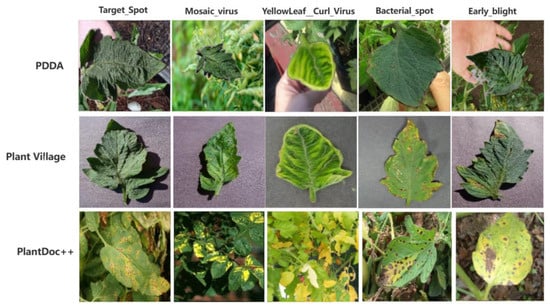
Figure 1.
Partial leaf comparison between PDDA, PlantVillage and PlantDoc++ datasets.
The idea of an inverted bottleneck module was proposed in the Transformer network and promoted in MobileNetV2 [29,30]. Additionally, the ConvNeXt network also adopts this structure as one of the basic structures in its ConvNeXt block. By using the inverted bottleneck structure, the amount of parameters of the whole ConvNeXt network is reduced, and the recognition accuracy is also improved [31]. The inverted bottleneck structure is the opposite of the bottleneck structure in that it has fewer input channels and fewer output channels than the number of channels in the intermediate convolutional layer. The following figure shows the ConvBN convolutional block that constitutes the IBSA module:
As shown in Figure 2, the ConvBN convolution block consists of a convolutional layer with a step number of 2 and a convolutional kernel size of 7 × 7, plus a BatchNorm layer with the activation function HardSwish. convBN 1 × 1 convolution is similar to ConvBN in that the convolutional layer uses 1 × 1 convolution for channel up-dimensioning and down-dimensioning. The convolutional kernel in ConvBN has a larger sensory field to extract more image information. BathNorm is a batch normalization operation that reduces the dependence of the model on the initial parameters and accelerates the network’s training and model generalization ability. In the design of the inverted bottleneck module, two models are used, including the maximum pooling layer (called IBMax) and without (called IB). The following figure shows the structure of the two modules.
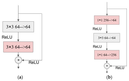
Figure 2.
Comparison of ResNet module before and after improvement (a) The module before improvement; (b) The module before improvement.
In the two inverted bottleneck introductory modules, the number of input and output channels of ConBN is c. The middle ConvBN1 × 1 and the third layer ConvBN1 × 1 channel up-dimensioning and down-dimensioning, respectively, and the up-dimensioning convolution changes the number of channels to four times the original one and then down-dimensioning back to c, Please refer to Figure 3 for detailed information and specifics. In the inverted bottleneck primary module with Maxpool, the changing pattern of the number of channels is the same as in Figure 4a.
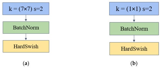
Figure 3.
ConvBN convolution block with ConvBN1 × 1 convolution that constitutes the inverted bottleneck of IBSA (a) ConvBN convolution block (b) ConvBN1 × 1 block.
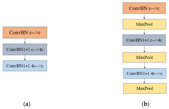
Figure 4.
Two inverted bottleneck master modules (a) Inverted bottleneck module (b)Inverted bottleneck module with MaxPool layer added.
3.2. Adding Shuffle Attention Module to Improve the Spatial Localization Accuracy of the Network for Sick Regions
For traditional convolutional networks, the spatial localization ability of the network is poor, i.e., the network cannot locate the leaf disease region well and learn the disease features during the recognition process. Shuffle Attention is one of the attention mechanisms, the core idea of which is to focus on the picture’s critical information [32]. The following Figure 5 shows the structure schematic of the Shuffle Attention module:
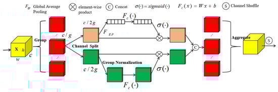
Figure 5.
Shuffle Attention module schematic.
The Shuffle Attention (from now on referred to as SA) module takes the given input , where C, H, and W denote the number of input channels, feature map height and width, respectively. SA divides the channels into g groups in the channel direction, i.e., , and for each , it generates two sub-feature maps by channel separation . As shown in Figure 4, after the channel separation, the upper branch outputs the channel attention map using the interrelationship between channels; the lower branch generates the spatial attention map using the feature space relationship.
- (1)
- Channel attention branch
Firstly, feature compression along the spatial dimension is performed by global average pooling to generate channel statistics s, for s there is , which embeds the global information of the feature subgraph. S is calculated as
s is multiplied with the initial feature subgraph after the operation and the sigmod activation function, and the final output is .
where , , which is in the same dimension as s, have the effect of scaling and panning the feature subgraphs.
- (2)
- Spatial attention branch
The spatial attention mechanism is more concerned with where the regions of interest are as a complement to the channel attention mechanism. The separated feature subgraphs are first subjected to the “Group Normalization” operation (GN) to obtain their spatial information, and then the feature representation is enhanced using the operation, and the final output is.
where, is shaped as .
The obtained channel attention and spatial attention branch outputs are finally stitched in the channel dimension, and two feature subgraphs with the number of channels C/2 g are stitched into a C/g channel subgraph. The feature subgraph that is divided into g groups, after the channel and spatial attention mechanism to the feature subgraph of , g feature subgraphs through the aggregation operation, recovered into the same latitude output as the initial input X ,. Finally, the aggregated output is then subjected to the channel shuffle operation, which enables cross-group communication of channel dimensions, enhances mutual learning between different information, and enhances the generalization of the model.
3.3. Enhancing Inter-Network Information Flow and Extraction by Building IBSA_Block
To better describe the model, the inverted bottleneck module (a) in Figure 4 that does not incorporate the maximum pooling layer is called IB_block, and (b) that incorporates the maximum pooling layer is called IBMax_block. By combining IB_block and IBMax_block with the SA module, together with the residual structure, the final model is composed of IBSA_Net shown in the following figure block; the final model uses the module composed of IBMax_block and SA, the structure is shown in Figure 6.
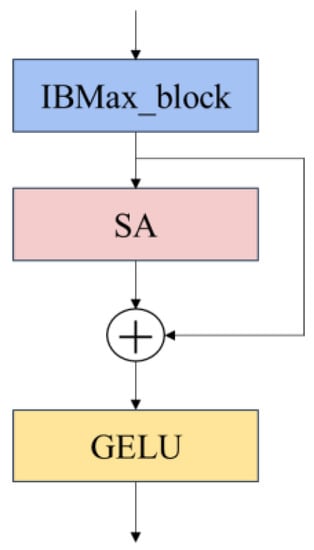
Figure 6.
IBSA_block module.
For the IBSA_block composed of IB_block and IB_Maxpool_block, there is no difference in the overall structure; both of them are input after IBMax_block, and then the disease area features are extracted by the SA attention mechanism module, and the output is summed with the branch shortcut to form the residual module. The final output goes through the activation function. The activation function between the IBSA_block block and the block is the GELU activation function.
3.4. IBSA_Net Overall Structure
The entire IBSA_Net forms the main structure by superimposing IBSA_block blocks three times, and the UP_convolution is used for channel up-convolution between IBSA_block blocks. The channel up-convolution uses a convolution kernel size of 1 × 1, and the number of output channels is twice the number of input channels. The final output uses global average pooling to extract the information and add the fully connected layer output. The following Figure 7 shows the structure of the entire IBSA_Net network Meanwhile, Table 2 shows the output dimensions of each module in IBSA_Net.
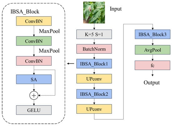
Figure 7.
IBSA_Net network structure.
Table 2.
Output dimensions of the different layers of IBSA_Net.
4. Experiment and Analysis
4.1. Experimental Configuration and Parameter Settings
This experiment uses Ubuntu 20.04.4 LTS 64 as the operating system (Canonical Ltd., London, UK) and Intel€ X€(R) Silver 4214 as the processor, CPU@2.20GHz, 32 G of RAM (Intel, Santa Clara, CA, USA). The GPU is an NVIDIA Tesla T4 with 16 G of video memory (Nvidia, Santa Clara, CA, USA).
In this paper, all experiments are conducted using stochastic gradient descent (SGD) with multiple batches. For the IBSA_Net network, the batch size (Batchsize) is set to 32; the number of training rounds epochs is 50; the optimizer adopts the SGD optimizer, the initial learning rate is 0.01, and the learning rate decay is used, the number of steps (step_size) is 2. The decay reduction factor lr_decay is 0.9. For every two training rounds, the learning rate is multiplied by the decay coefficient. The cross-entropy loss function is used for the loss function.
4.2. Evaluation Indicators
To better evaluate the performance of different models on the same dataset, the following metric is considered to be introduced to evaluate the models: accuracy, which calculates the number of correctly predicted samples as a proportion of the total number of samples, as shown in Equation (4). Precision is the probability that, given a positive label, how many of them are true positives, i.e., the ratio of correctly predicted positive samples to the total number of predicted positive samples, as shown in Equation (5). The recall is the accuracy of predicting positive sample instances, i.e., the ratio of correctly predicted positive samples to the total number of actual positive samples, as shown in Equation (6). the F1 score integrates Precision and Recall to reconcile both, as shown in Equation (7).
In the network training process of deep learning, the loss function calculates the gap between the actual value and the predicted value. The one used in this paper is the cross-entropy loss function with the following equation.
where is the expected probability of the input and is the actual probability of the input. The smaller the L obtained from both calculations, the smaller the difference between the actual value and the predicted value, and the more accurate the prediction is.
4.3. Ablation Experiments of Model Lifting by Key Modules
In this subsection, the critical modules mentioned are the HardSwish activation function, the IBMax module, and the Shuffle-Attention module. We refer to the model in which all key modules are removed as OriNet.
The addition of activation functions can add nonlinear factors to the network and increase the expressive power of the neural network. The HardSwish (HS) function was first proposed in the MobileNetV3 model [33]. Compared with the traditional Swish activation function, the HardSwish activation function is faster to compute and has better numerical stability. For the HardSwish function, the equation is as follows.
It extracts the primary information in the image for the maximum pooling layer. It makes the feature map of the image to operate in the network smaller, making the information denser while reducing the number of operations.
The following table shows the increase and decrease in comprehensive training and testing accuracy due to the addition and removal of the three key modules and the comparison of recognition accuracy.
As seen in Table 3, each of the three key modules contributes to the network, and adding any of the three modules improves network performance. The IBMax module has the most significant improvement for the first three individual module additions. The performance improvement from adding two key modules is more significant than that from adding only one. The above experimental results show that our proposed key modules effectively improve the network performance, which eventually brings a 9.2% performance improvement.
Table 3.
Effect of different key modules on model accuracy.
4.4. Comparison Experiments of Model Clusters with Different Datasets
In this study, the performance of the PlantVillage model group was analyzed in terms of training and testing. The recognition accuracy of six models was evaluated using the accuracy curve shown in Figure 8a,b. The findings revealed that the IBSA_Net model outperformed the other models, exhibiting significantly higher recognition accuracy in the early stages of training. As the training progressed, the accuracy curve of IBSA_Net tended to flatten after eth 10th round, indicating a convergence effect. After 50 rounds of training, the IBSA_Net model achieved a training accuracy of 99.7% and a testing accuracy of 99.4%. While the EfficientNet and MobileNetV3 models showed similar training accuracy to IBSA_Net in eth 50th round, at 98.4% and 97.6%, respectively, the training and testing accuracy gaps of models other than IBSA_Net were over 2%. These findings suggest that these models suffer from overfitting problems and display weaker generalization ability than the IBSA_Net model.
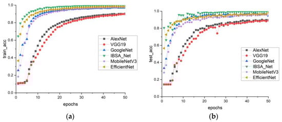
Figure 8.
Comparison of accuracy of PlantVillage model clusters (a) train_acc, (b) test_acc.
In Figure 9a,b, the performance of six models on the PDDA dataset is evaluated. The results demonstrate that the training and testing accuracies of all models have decreased compared to those of PlantVillage. This decline in accuracy may be due to the greater complexity of the backgrounds in the PDDA dataset. However, IBSA_Net remains the best-performing model, indicating its ability to remain less influenced by complex backgrounds and display stronger robustness than the other models.
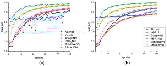
Figure 9.
PDDA model cluster accuracy comparison (a) train_acc, (b) test_acc.
Table 4 and Table 5 illustrate that the proposed IBSA_Net model exhibits superior performance on both the PlantVillage and PDDA datasets. Compared to advanced models, such as EfficientNet and MobileNetV3, along with classical convolutional neural networks, IBSA_Net achieves higher accuracy, precision, and recall scores. Moreover, IBSA_Net shows excellent performance in leaf recognition tasks under complex backgrounds.
Table 4.
PlantVillage Model Cluster Evaluation Metrics.
Table 5.
PDDA model cluster evaluation metrics.
In Figure 10, the loss curve graph reveals that IBSA_Net has the smallest loss and converges the fastest. After eth 10th round of training, the loss curve of IBSA_Net begins to flatten, while the training losses of the other five models in the first five rounds are significantly larger than those of IBSA_Net.
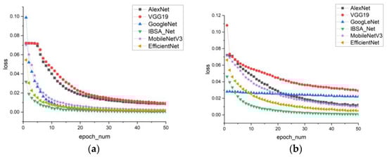
Figure 10.
Training loss (a) PlantVillage model cluster (b) PDDA model cluster.
4.5. Transfer Learning with Small Sample Datasets PlantDoc++
Generally speaking, it is more difficult to obtain many crop disease leaf datasets in natural environments, especially for the nine tomato leaf disease datasets in this paper. Although there are more large public datasets available for people to use, the leaves in the public dataset represented by PlantVillage are primarily taken in a single background, which does not reflect the pose of leaves in the natural environment and is almost noiseless data. The models trained on such datasets cannot be extended to use in natural agricultural production environments. So this paper uses the PDDA dataset to simulate the natural picking environment. The PDDA dataset is to segment the leaves in the public dataset. It moves them to the background map of the natural tomato planting and picking environment to try to fit the tomato leaves in the natural environment, increase the noise of the dataset, and make the model more robust to the recognition of complex backgrounds and leaves.
Afterward, using the idea of transfer learning, the model clusters trained on PlantVillage and PDDA datasets, respectively, retaining their model parameters, were trained on the small sample dataset PlantDoc++ before testing the accuracy of the two model clusters in identifying tomato leaf diseases in natural environments.
The tomato leaf categories represented by the 0 to 9 markers in Figure 11 correspond to the leaf categories from Bacterial_spot to healthy in Table 6. Figure 11 and Table 6 show that the PlantVillage model cluster has a more significant decrease in the ability to identify disease datasets in natural environments compared to PlantVillage, with a generally low recall rate. However, the IBSA_Net network still has the best performance among all models. This indicates that after transfer learning, IBSA_Net pays more attention to the leaf features and has stronger robustness.
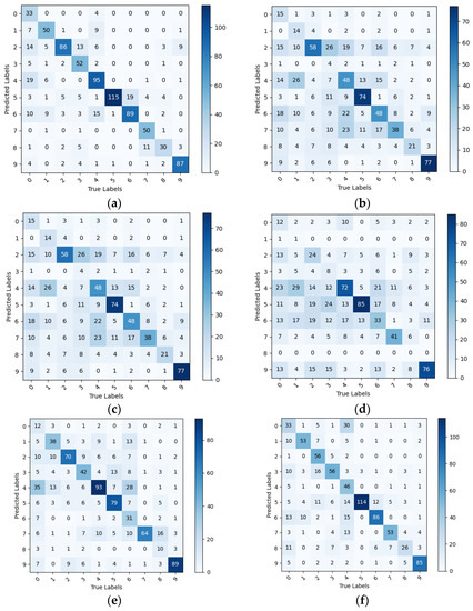
Figure 11.
Confusion matrix for PlantVillage model cluster tested on PlantDoc++, (a) IBSA_Net (b) AlexNet (c) VGG (d) Goog€et (e) MobileNetV3 (f) EfficientNet.
Table 6.
Comparison of evaluation metrics of PlantVillage model clusters on PlantDoc++.
Table 6.
Comparison of evaluation metrics of PlantVillage model clusters on PlantDoc++.
| IBSA_Net | Precision | Recall | F1-Score | AlexNet | Precision | Recall | F1-Score |
|---|---|---|---|---|---|---|---|
| Bacterial spot | 0.892 | 0.344 | 0.496 | 0.739 | 0.183 | 0.293 | |
| Early blight | 0.735 | 0.685 | 0.709 | 0.656 | 0.583 | 0.617 | |
| Late blight | 0.632 | 0.851 | 0.725 | 0.69 | 0.58 | 0.630 | |
| Leaf Mold | 0.825 | 0.627 | 0.712 | 0.596 | 0.415 | 0.489 | |
| Septoria leaf_spot | 0.779 | 0.714 | 0.745 | 0.451 | 0.667 | 0.538 | |
| Spider mites | 0.732 | 0.983 | 0.839 | 0.601 | 0.819 | 0.693 | |
| Target Spot | 0.674 | 0.824 | 0.741 | 0.488 | 0.738 | 0.587 | |
| Yellow Leaf Curl Virus | 0.943 | 0.746 | 0.833 | 0.538 | 0.424 | 0.474 | |
| Mosaic virus | 0.577 | 0.698 | 0.631 | 0.481 | 0.619 | 0.541 | |
| healthy | 0.853 | 0.861 | 0.856 | 1 | 0.61 | 0.757 | |
| avg | 0.764 | 0.733 | 0.728 | 0.624 | 0.563 | 0.562 | |
| VGG | precision | recall | F1-score | GoogLeNet | precision | recall | F1-score |
| Bacterial spot | 0.577 | 0.161 | 0.252 | 0.188 | 0.548 | 0.280 | |
| Early blight | 0.609 | 0.194 | 0.294 | 0.2 | 0.014 | 0.026 | |
| Late blight | 0.345 | 0.58 | 0.433 | 0.338 | 0.27 | 0.300 | |
| Leaf Mold | 0.333 | 0.049 | 0.085 | 1.0 | 0.024 | 0.047 | |
| Septoria leaf_spot | 0.366 | 0.364 | 0.365 | 0.345 | 0.227 | 0.274 | |
| Spider mites | 0.649 | 0.638 | 0.643 | 0.818 | 0.078 | 0.142 | |
| Target Spot | 0.35 | 0.449 | 0.393 | 0.5 | 0.065 | 0.115 | |
| Yellow Leaf Curl Virus | 0.295 | 0.576 | 0.390 | 0.278 | 0.682 | 0.395 | |
| Mosaic virus | 0.318 | 0.5 | 0.389 | 0.182 | 0.095 | 0.125 | |
| healthy | 0.74 | 0.77 | 0.755 | 0.312 | 0.8 | 0.449 | |
| avg | 0.458 | 0.428 | 0.399 | 0.416 | 0.280 | 0.215 | |
| MobileNetV3 | precision | recall | F1-score | EfficientNet | precision | recall | F1-score |
| Bacterial spot | 0.5 | 0.125 | 0.200 | 0.434 | 0.344 | 0.384 | |
| Early blight | 0.507 | 0.521 | 0.514 | 0.679 | 0.726 | 0.702 | |
| Late blight | 0.579 | 0.693 | 0.631 | 0.875 | 0.554 | 0.678 | |
| Leaf Mold | 0.5 | 0.506 | 0.503 | 0.583 | 0.675 | 0.626 | |
| Septoria leaf spot | 0.489 | 0.699 | 0.575 | 0.821 | 0.346 | 0.487 | |
| Spider mites | 0.675 | 0.675 | 0.675 | 0.651 | 0.974 | 0.780 | |
| Target Spot | 0.66 | 0.287 | 0.400 | 0.672 | 0.796 | 0.729 | |
| Yellow Leaf Curl Virus | 0.52 | 0.955 | 0.673 | 0.646 | 0.791 | 0.711 | |
| Mosaic virus | 0.5 | 0.233 | 0.318 | 0.4 | 0.605 | 0.482 | |
| healthy | 0.736 | 0.881 | 0.802 | 0.833 | 0.842 | 0.837 | |
| avg | 0.566 | 0.557 | 0.529 | 0.659 | 0.6653 | 0.641 |
In the PDDA model group, all models exhibited higher evaluation metrics than the PlantVillage model group, thus confirming the previous hypothesis that pre-training on datasets that simulate complex backgrounds can enhance a model’s ability to distinguish leaves from backgrounds and reduce interference from background factors. Although EfficientNet achieved precision and recall scores of 1 for certain diseases, its average values for all evaluation metrics were lower than those of IBSA_Net. Specifically, its evaluation metrics were lower for certain diseases, indicating that the model may have higher recognition rates for specific disease categories while lower recognition rates for others, which is not suitable for actual agricultural production environments. By contrast, the proposed IBSA_Net model in this study has almost no imbalanced evaluation metrics, displaying high evaluation metrics for each disease category. Moreover, IBSA_Net exhibits excellent transfer learning ability, demonstrating strong knowledge transfer from the source domain to the target domain. After pre-training on PDDA and testing on PlantDoc++, IBSA_Net achieved average precision, recall, and F1-score values of 0.942, 0.944, and 0.943, respectively, which were higher than the average evaluation metric values of the other five networks. Please refer to Figure 12 and Table 7 for detailed information and specifics.
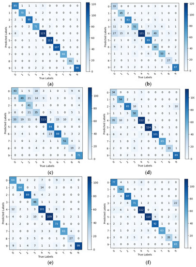
Figure 12.
Confusion matrix for PDDA model clusters tested on PlantDoc++, (a) IBSA_Net (b) AlexNet (c) VGG (d) GoogLeNet (e)MobileNetV3 (f) EfficientNet.
Table 7.
Comparison of evaluation metrics of PDDA model clusters on PlantDoc++.
4.6. Attentional Visualization Experiment
In order to better understand how convolutional neural networks identify diseases in different parts of the images during training, this paper utilizes the Grad-CAM attention visualization tool to generate attention heat maps of the network’s predictions [34,35]. The heat map highlights important regions by color-coding them, where redder and warmer colors correspond to regions of greater importance that the network is most interested in, while cooler colors (bluish) denote regions of less interest. Attention visualizations were obtained for some diseased leaves, and the corresponding heat maps are shown in Figure 13. From the heat maps, we can observe that within the PlantVillage model cluster, the red areas of the three models, except IBSA_Net, are small and scattered. In contrast, the warm areas of the IBSA_Net network are mainly concentrated around the disease spots, but the attention is not focused on the disease spot area. This indicates that the disease information learned from a single background dataset may not generalize well to more complex background datasets.
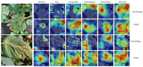
Figure 13.
Attentional heat map, PlantVillage represents the PlantVillage model group; PDDA represents the PDDA model group.
It is important to note that in the first attention heat map of early blight, GoogLeNet and VGG networks identified non-disease areas, such as the hole formed by the branch in the upper left corner and the overlap of the leaf edge and background, as diseased spots. As depicted in the figure, these networks tend to show “false spots” in red regions of their attention heat maps. In contrast, after pre-training on the PDDA dataset, IBSA_Net demonstrated a superior ability to distinguish between “false spots” and actual diseased regions. The attention heat map of IBSA_Net mostly identifies diseased spots, assigning higher attention weights to these regions. The “false spots” related to the holes formed by the branch are colored light yellow and cyan, indicating lower network attention to these areas. Similarly, in the Target_Spot dataset, IBSA_Net effectively avoided predicting shadows or non-disease black spots as diseased regions, whereas other networks made such errors. These findings suggest that IBSA_Net can self-learn the differences between diseased regions and the environmental illusions of leaves and better distinguish between them.
Conversely, in the PDDA model cluster, there are significantly more warm regions in the attention heat maps and more overlap with the disease spot region. Precisely, the warm color regions of IBSA_Net largely overlap with the disease spot regions and cover most of the spots. This suggests that the ability to distinguish complex backgrounds from leaf spot regions was learned from the PDDA dataset and that IBSA_Net had the most significant ability to generalize from the source domain to the target domain.
To further quantify the level of attention each model pays to the diseased regions of tomato leaves, we calculated the percentage of warm regions versus diseased regions for each model’s attention visualization when predicting the PlantDoc++ test set after training on different datasets. The attention matrix was converted to a NumPy array format, reshaped to the same size as the original image, and then superimposed on the original image to generate a visualized attention map. The number of pixels in the attention map was calculated based on the location of the tomato leaf spots or the bounding box [36]. The number of pixels in the warm area of the attention map was determined by applying a set threshold. Finally, the ratio of the number of pixels of the object to be recognized to the number of pixels in the warm area was obtained.
Table 8 displays the attention level of each model for the two tomato leaf diseases, Early_blight and Target_Spot, depicted in Figure 13. For both diseases, the PDDA model group has a higher proportion of warm-colored regions covered in the attention heat map compared to the PlantVillage model group. Furthermore, the area percentage of IBSA_Net, proposed in this paper, has the highest value in all the results.
Table 8.
Percentage of warm and sick areas in the attentional heat map.
4.7. Performance of IBSA_Net on Other Crops
While the experiments conducted in this study primarily focused on tomato disease leaves, the feature extraction and identification capabilities of IBSA_Net can be extended to other crops. To test this, we evaluated the model’s performance on apple and chili pepper leaves, the dataset examples are shown in Figure 14 and Figure 15. The apple leaf dataset comprises five categories: Alternaria leaf spot, Brown spot, Grey spot, Mosaic, and Healthy, while the chili pepper leaf dataset consists of two categories: Bacterial spot and Healthy. These datasets were obtained from Yang’s paper and PlantVillage, respectively [37]. The datasets were split into an 8:2 ratio for training and testing, and the results are presented below.
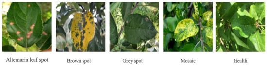
Figure 14.
Apple leaf disease dataset.
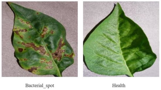
Figure 15.
Pepper leaf disease dataset.
From Table 9 and Table 10, it is evident that both IBSA_Net and EfficientNet outperformed the other four models. Although EfficientNet achieved 0.7% higher accuracy than IBSA_Net on the apple leaf disease dataset, IBSA_Net exhibited superior performance in terms of Precision, Recall, and F1-score evaluation metrics. Furthermore, on the pepper leaf disease dataset, IBSA_Net outperformed all other five networks in all evaluation metrics. The results obtained from the apple and pepper leaf datasets confirm the efficacy of IBSA_Net in recognizing diseases in different crops. Remarkably, IBSA_Net demonstrated remarkable disease recognition and generalization abilities, even in the presence of complex image backgrounds.
Table 9.
Performance of the six models on the apple leaf data set.
Table 10.
Performance of the six models on the pepper leaf disease dataset.
5. Conclusions
The IBSA_Net proposed in this study combines the inverted bottleneck network and Shuffle Attention mechanism while also incorporating the HardSwish activation function, IBMax, and other modules. By doing so, the proposed network achieves not only superior recognition accuracy but also a faster convergence speed. In addition, it can extract multi-scale plant disease spot features, accurately locate disease areas, and identify tomato leaf diseases with fine granularity.
To address the issue of the limited generalization ability of models trained on a single background dataset in natural agricultural production environments, we propose a transfer learning-based training method for small sample datasets. Specifically, we utilize the PDDA dataset, which simulates a complex natural background, to pre-train the model clusters. Experimental results demonstrate that the pre-trained IBSA_Net on PDDA achieves the best performance on the real dataset. The mean values of 0.942, 0.944, and 0.943 for the precision, recall, and F1-score, respectively, highlight the effectiveness of our approach.
In addition, the results of attention visualization experiments demonstrated that the PDDA model group exhibited a significantly larger warm-colored area overlapping with the lesions compared to the PlantVillage model group. Moreover, the IBSA_Net disease recognition area demonstrated the highest overlap with the entire lesion area of the leaf while also exhibiting a good ability to differentiate between “false lesions” and real lesion areas. Finally, we tested the performance of IBSA_Net on other crops and achieved good results. These findings suggest that our model and methodology offer an effective and reliable approach to identifying leaf diseases in complex backgrounds, with potential applicability to other crops. Nonetheless, this study has certain limitations. Due to the challenges associated with collecting tomato leaf datasets, there is a paucity of tomato leaf samples exhibiting growth defects caused by nutritional deficiencies. Furthermore, in actual agricultural production, some symptoms of viral diseases are akin to those caused by nutritional deficiencies, leading to network misjudgment and the incorrect identification of nutrient-deficient leaves as disease-afflicted. In future work, we will gather additional tomato leaf samples with growth defects resulting from different causes and refine the model proposed herein to enable better differentiation of these variations.
Author Contributions
Conceptualization, R.Z. and Y.W.; methodology, R.Z. and Y.W.; software, J.P.; validation, R.Z., H.C. and J.P.; data curation, H.C.; writing—original draft preparation, R.Z.; writing—review and editing, Y.W.; visualization, P.J.; funding acquisition and supervision, Y.W. and P.J. All authors have read and agreed to the published version of the manuscript.
Funding
This research was funded by the National Key R&D Program of China under the sub-project “Research and System Development of Navigation Technology for Harvesting Machine of Special Economic Crops” (No. 2022YFD2002001) within the key program “Engineering Science and Comprehensive Interdisciplinary Research”.
Institutional Review Board Statement
Not applicable.
Informed Consent Statement
Not applicable.
Data Availability Statement
The public datasets used in this paper can be accessed through the following links: Plant Village: https://www.kaggle.com/datasets/abdallahalidev/plantvillage-dataset (accessed on 27 March 2023); PlantVillage Dataset with Data Augmentation(PDDA): https://www.kaggle.com/datasets/alessandrobiz/plantvillage-dataset-with-data-augmentation (accessed on 27 March 2023), PlantDoc [21]: https://github.com/pratikkayal/PlantDoc-Dataset (accessed on 27 March 2023), AppleLeaf9 [31]: https://github.com/JasonYangCode/AppleLeaf9 (accessed on 27 March 2023).
Conflicts of Interest
The authors declare no conflict of interest.
References
- Ferdouse Ahmed Foysal, M.; Shakirul Islam, M.; Abujar, S.; Akhter Hossain, S. A novel approach for tomato diseases classification based on deep convolutional neural networks. In Proceedings of the International Joint Conference on Computational Intelligence: IJCCI 2018, Birulia, Bangladesh, 2–4 November 2020; pp. 583–591. [Google Scholar]
- Yuan, Y.; Chen, L.; Wu, H.; Li, L. Advanced agricultural disease image recognition technologies: A review. Inf. Process. Agric. 2022, 9, 48–59. [Google Scholar] [CrossRef]
- Aravind, K.R.; Maheswari, P.; Raja, P.; Szczepański, C. Crop disease classification using deep learning approach: An overview and a case study. In Deep Learning for Data Analytics; Elsevier: Amsterdam, The Netherlands, 2020; pp. 173–195. [Google Scholar]
- Barbedo, J.G. Factors influencing the use of deep learning for plant disease recognition. Biosyst. Eng. 2018, 172, 84–91. [Google Scholar] [CrossRef]
- Jiang, F.; Lu, Y.; Chen, Y.; Cai, D.; Li, G. Image recognition of four rice leaf diseases based on deep learning and support vector machine. Comput. Electron. Agric. 2020, 179, 105824. [Google Scholar] [CrossRef]
- Rangarajan, A.K.; Purushothaman, R.; Prabhakar, M.; Szczepański, C. Crop identification and disease classification using traditional machine learning and deep learning approaches. J. Eng. Res. 2021. [Google Scholar] [CrossRef]
- Abade, A.; Ferreira, P.A.; de Barros Vidal, F. Plant diseases recognition on images using convolutional neural networks: A systematic review. Comput. Electron. Agric. 2021, 185, 106125. [Google Scholar] [CrossRef]
- Waheed, A.; Goyal, M.; Gupta, D.; Khanna, A.; Hassanien, A.E.; Pandey, H.M. An optimized dense convolutional neural network model for disease recognition and classification in corn leaf. Comput. Electron. Agric. 2020, 175, 105456. [Google Scholar] [CrossRef]
- Zeng, W.; Li, M. Crop leaf disease recognition based on Self-Attention convolutional neural network. Comput. Electron. Agric. 2020, 172, 105341. [Google Scholar] [CrossRef]
- Annabel, L.S.P.; Muthulakshmi, V. AI-powered image-based tomato leaf disease detection. In Proceedings of the Third International Conference on I-SMAC (IoT in Social, Mobile, Analytics and Cloud) (I-SMAC), Palladam, India, 12–14 December 2019; pp. 506–511. [Google Scholar]
- Das, D.; Singh, M.; Mohanty, S.S.; Chakravarty, S. Leaf disease detection using support vector machine. In Proceedings of the International Conference on Communication and Signal Processing (ICCSP), Chennai, India, 28–30 July 2020; pp. 1036–1040. [Google Scholar]
- Thangaraj, R.; Anandamurugan, S.; Kaliappan, V.K. Automated tomato leaf disease classification using transfer learning-based deep convolution neural network. J. Plant Dis. Prot. 2021, 128, 73–86. [Google Scholar] [CrossRef]
- Zhang, P.; Yang, L.; Li, D. EfficientNet-B4-Ranger: A novel method for greenhouse cucumber disease recognition under natural complex environment. Comput. Electron. Agric. 2020, 176, 105652. [Google Scholar] [CrossRef]
- Tang, Z.; Yang, J.; Li, Z.; Qi, F. Grape disease image classification based on lightweight convolution neural networks and channelwise attention. Comput. Electron. Agric. 2020, 178, 105735. [Google Scholar] [CrossRef]
- Barman, U.; Choudhury, R.D.; Sahu, D.; Barman, G.G. Comparison of convolution neural networks for smartphone image based real time classification of citrus leaf disease. Comput. Electron. Agric. 2020, 177, 105661. [Google Scholar] [CrossRef]
- Gonzalez-Huitron, V.; León-Borges, J.A.; Rodriguez-Mata, A.; Amabilis-Sosa, L.E.; Ramírez-Pereda, B.; Rodriguez, H. Disease detection in tomato leaves via CNN with lightweight architectures implemented in Raspberry Pi 4. Comput. Electron. Agric. 2021, 181, 105951. [Google Scholar] [CrossRef]
- Abbas, A.; Jain, S.; Gour, M.; Vankudothu, S. Tomato plant disease detection using transfer learning with C-GAN synthetic images. Comput. Electron. Agric. 2021, 187, 106279. [Google Scholar] [CrossRef]
- Brahimi, M.; Boukhalfa, K.; Moussaoui, A. Deep learning for tomato diseases: Classification and symptoms visualization. Appl. Artif. Intell. 2017, 31, 299–315. [Google Scholar] [CrossRef]
- Ullah, Z.; Alsubaie, N.; Jamjoom, M.; Alajmani, S.H.; Saleem, F. EffiMob-Net: A Deep Learning-Based Hybrid Model for Detection and Identification of Tomato Diseases Using Leaf Images. Agriculture 2023, 13, 737. [Google Scholar] [CrossRef]
- Waheed, H.; Akram, W.; Islam, S.u.; Hadi, A.; Boudjadar, J.; Zafar, N. A Mobile-Based System for Detecting Ginger Leaf Disorders Using Deep Learning. Future Internet 2023, 15, 86. [Google Scholar] [CrossRef]
- Ulutaş, H.; Aslantaş, V. Design of Efficient Methods for the Detection of Tomato Leaf Disease Utilizing Proposed Ensemble CNN Model. Electronics 2023, 12, 827. [Google Scholar] [CrossRef]
- Luo, Y.; Cai, X.; Qi, J.; Guo, D.; Che, W. FPGA–accelerated CNN for real-time plant disease identification. Comput. Electron. Agric. 2023, 207, 107715. [Google Scholar] [CrossRef]
- Fan, X.; Luo, P.; Mu, Y.; Zhou, R.; Tjahjadi, T.; Ren, Y. Leaf image based plant disease identification using transfer learning and feature fusion. Comput. Electron. Agric. 2022, 196, 106892. [Google Scholar] [CrossRef]
- Janarthan, S.; Thuseethan, S.; Rajasegarar, S.; Yearwood, J. P2OP—Plant Pathology on Palms: A deep learning-based mobile solution for in-field plant disease detection. Comput. Electron. Agric. 2022, 202, 107371. [Google Scholar] [CrossRef]
- Jiang, D.; Li, F.; Yang, Y.; Yu, S. A tomato leaf diseases classification method based on deep learning. In Proceedings of the Chinese Control and Decision Conference (CCDC), Hefei, China, 22–24 August 2020; pp. 1446–1450. [Google Scholar]
- Rubanga, D.P.; Loyani, L.K.; Richard, M.; Shimada, S. A deep learning approach for determining effects of Tuta Absoluta in tomato plants. arXiv 2020, arXiv:2004.04023. [Google Scholar]
- Singh, D.; Jain, N.; Jain, P.; Kayal, P.; Kumawat, S.; Batra, N. PlantDoc: A dataset for visual plant disease detection. In Proceedings of the 7th ACM IKDD CoDS and 25th COMAD, Hyderabad, India, 5–7 January 2020; pp. 249–253. [Google Scholar]
- He, K.; Zhang, X.; Ren, S.; Sun, J. Deep residual learning for image recognition. In Proceedings of the IEEE Conference on Computer Vision and Pattern Recognition, Las Vegas, NV, USA, 27–30 June 2016; pp. 770–778. [Google Scholar]
- Sandler, M.; Howard, A.; Zhu, M.; Zhmoginov, A.; Chen, L.-C. Mobilenetv2: Inverted residuals and linear bottlenecks. In Proceedings of the IEEE Conference on Computer Vision and Pattern Recognition, Salt Lake City, UT, USA, 18–23 June 2018; pp. 4510–4520. [Google Scholar]
- Vaswani, A.; Shazeer, N.; Parmar, N.; Uszkoreit, J.; Jones, L.; Gomez, A.N.; Kaiser, Ł.; Polosukhin, I. Attention is all you need. Adv. Neural Inf. Process. Syst. 2017, 30, 1–11. [Google Scholar]
- Liu, Z.; Mao, H.; Wu, C.-Y.; Feichtenhofer, C.; Darrell, T.; Xie, S. A convnet for the 2020s. In Proceedings of the IEEE/CVF Conference on Computer Vision and Pattern Recognition, New Orleans, LA, USA, 18–24 June 2022; pp. 11976–11986. [Google Scholar]
- Zhang, Q.-L.; Yang, Y.-B. Sa-net: Shuffle attention for deep convolutional neural networks. In Proceedings of the ICASSP 2021—IEEE International Conference on Acoustics, Speech and Signal Processing (ICASSP), Toronto, ON, Canada, 6–11 June 2021; pp. 2235–2239. [Google Scholar]
- Howard, A.; Sandler, M.; Chu, G.; Chen, L.-C.; Chen, B.; Tan, M.; Wang, W.; Zhu, Y.; Pang, R.; Vasudevan, V. Searching for mobilenetv3. In Proceedings of the IEEE/CVF International Conference on Computer Vision, Seoul, Republic of Korea, 27–28 October 2019; pp. 1314–1324. [Google Scholar]
- An, J.; Joe, I. Attention Map-Guided Visual Explanations for Deep Neural Networks. Appl. Sci. 2022, 12, 3846. [Google Scholar] [CrossRef]
- Selvaraju, R.R.; Cogswell, M.; Das, A.; Vedantam, R.; Parikh, D.; Batra, D. Grad-cam: Visual explanations from deep networks via gradient-based localization. In Proceedings of the IEEE International Conference on Computer Vision, Venice, Italy, 22–29 October 2017; pp. 618–626. [Google Scholar]
- Redmon, J.; Divvala, S.; Girshick, R.; Farhadi, A. You only look once: Unified, real-time object detection. In Proceedings of the IEEE Conference on Computer Vision and Pattern Recognition, Las Vegas, NV, USA, 27–30 June 2016; pp. 779–788. [Google Scholar]
- Yang, Q.; Duan, S.; Wang, L. Efficient Identification of Apple Leaf Diseases in the Wild Using Convolutional Neural Networks. Agronomy 2022, 12, 2784. [Google Scholar] [CrossRef]
Disclaimer/Publisher’s Note: The statements, opinions and data contained in all publications are solely those of the individual author(s) and contributor(s) and not of MDPI and/or the editor(s). MDPI and/or the editor(s) disclaim responsibility for any injury to people or property resulting from any ideas, methods, instructions or products referred to in the content. |
© 2023 by the authors. Licensee MDPI, Basel, Switzerland. This article is an open access article distributed under the terms and conditions of the Creative Commons Attribution (CC BY) license (https://creativecommons.org/licenses/by/4.0/).