Abstract
In this study, dynamic characteristics of a composite beam with uncertain design parameters are analyzed. Uncertain-but-bounded parameters change only within certain specified limits. This study uses interval analysis to investigate a composite beam with viscoelastic layers whose behavior is described using the fractional Zener model. In general, parameters describing both elastic and viscoelastic layers can be uncertain. Several methods have been studied to determine the lower and upper bounds of the dynamic characteristics of a structure. Among them, the vertex method is a comparative method in which the lower and upper bounds of the dynamic characteristics are approximated using the first- and second-order Taylor series expansion. An algorithm to determine the critical combination of uncertain design parameters has also been described. Numerical examples demonstrate the effectiveness of the presented methods and the possibility of applying them to the analysis of systems with numerous uncertain parameters and high uncertainties.
1. Introduction
An important issue while solving engineering-related problems is taking into account the uncertainty of design parameters. Many parameters may have physical and geometric uncertainties as a result of modeling inaccuracies, measurement errors, manufacturing errors, etc. Parameter uncertainties can be dealt with using three methods: probabilistic methods, fuzzy theory, and interval values. In probabilistic methods, the parameters are described as random variables, assuming that the probability distribution is known. Some examples of probabilistic methods are the Monte Carlo method [1], perturbation techniques [2], and spectral methods [3]. However, probabilistic methods are often labor intensive. The fuzzy theory method is used to analyze uncertainties especially when sufficiently reliable stochastic data are not available [4]. In the interval values method, uncertainties are modeled as interval values, whose parameters are uncertain but bounded.
In 1979, Moore [5] introduced the concept of interval analysis. Since then, this method has been used to address numerous static and dynamic problems. In [6], interval analysis was used to solve the eigenproblem of systems with uncertain parameters. The interval finite element method was used in [7,8], where the eigenvalue problem of systems with parameters described by interval values was addressed. The mass and stiffness matrices were expressed using the matrix perturbation theory. In [9], this method was applied in damped systems. In [10], it was demonstrated that the range of the structure response obtained using the perturbation theory, together with the interval analysis, includes the range obtained by the probabilistic method.
In [11], the modal interval analysis method was used to analyze natural frequencies, eigenvectors, and frequency response functions.
The solution for systems with uncertain-but-bounded parameters can also be determined using the vertex method [12,13]. This method assumes that the solution is sought only for the limit values of the parameters and consists in solving the problem for each combination of them. Thus, it is necessary to select the lower and upper limits of the structure response among the solutions obtained. This method yields an exact or close-to-exact solution but is labor intensive as it requires 2r combinations of parameters (where r is the number of uncertain parameters).
Hence, numerous other methods for calculating the lower and upper bounds of the response function have recently been proposed. In [14], to determine natural frequencies, a combination of the interval finite element method with the element-by-element approach was presented. The advantage of this approach is that overestimation of the obtained solution is prevented. A similar approach was used in [15] to determine the lower and upper limits of frequency response functions. In this approach, equations describing the dynamic response of the structure are written as a system of interval linear equations, which is solved iteratively using Brouwer’s fixed-point theorem. In [16], the frequency response function was analyzed using the Laplace transform, but this method is suitable only for small uncertainties. In [17], a method for deriving approximate explicit expressions of frequency response functions was presented.
In [18], the time response of a structure with uncertainties that are described as random and/or interval quantities was presented. In this study, three models of uncertainty were proposed: the first applied the generalized polynomial chaos theory to uncertainties described as random quantities, the second used the Legendre metamodel to uncertainties described as interval quantities, whereas the third was a hybrid one that takes into account the possibility of both random and interval uncertainties.
In [19], the dynamic response of the structure, which is subjected to uncertain excitations, was analyzed. In this method, quadratic programming with a bivalent constraint at each time point was applied to determine the response limit of the structure. Uncertain-but-bounded external loads were analyzed in [20], in which a nonprobability modal superposition method was proposed. The obtained solution area was wider than that in the case of using the probabilistic approach, but this method was definitely less laborious. In [21], Chebyshev polynomials were used to estimate the limits of the dynamic response of systems with uncertain parameters.
Furthermore, the lower and upper limits of the structure response can be obtained by expanding the expected value into a Taylor series, as shown in [22], in which the Taylor series expansion was used to estimate the range of the nonlinear response of the structure with uncertainties. The second-order Taylor series expansion was used in [23] to determine the limits of natural frequencies. In [24], the second-order Taylor series expansion was used to determine the critical combination of uncertain parameters, i.e., the combination for which the structure response takes the minimum and maximum values. In addition, this method does not require much computational effort. The first- and second-order Taylor series expansion was also used in [25], where the solution of the eigenvalue problem and frequency response functions for systems with viscoelastic dampers were analyzed. In [26], uncertainties of a system with viscoelastic dampers were analyzed using a probabilistic approach.
In [27], stochastic analysis was applied to systems with uncertain-but-bounded parameters. This method adopted a first-order approximation of the random response obtained by improving the interval analysis based on affine arithmetic. In [28], a hybrid stochastic and interval approach was used to analyze systems with mixed random and interval parameters. The expressions of mean values and the variance of the considered quantity were derived using the perturbation method and the random interval moment method. Interval analysis was used to determine the limits of these probabilistic quantities. The advantage of this approach is that it can be applied to all of the following scenarios: only random, only interval, and mixed parameters.
Interval analysis can also be applied to problems related to the structure design process. In [29,30], it was used to optimize systems with uncertainties, whereas in [31], it was used to analyze the nodes of the structure subjected to dynamic effects. Interval analysis was also used to model the nodes of the structure and hence to find the connections whose stiffness change would have a positive effect on the structure response. Furthermore, it was used in the analysis of systems with uncertainties that use an active vibration control system [32].
In Table 1, a brief overview as well as the advantages and disadvantages of three main groups of methods used for analyzing systems with uncertainties are presented. It is worth noting that the choice of an appropriate method depends on the nature of the problem and the available data.

Table 1.
Methods used for the analysis of systems with uncertainties.
In this study, a composite beam with viscoelastic layers was considered. It is assumed that design parameters change within certain specified limits. Interval analysis was used to determine the dynamic response of the structure in the form of dynamic characteristics. Their limits were expressed as the first- and second-order Taylor series expansions. The solutions obtained were compared with those calculated using the vertex method, which can be adopted as a comparative method. This study also presented an algorithm that can obtain a critical combination of uncertain parameters, just like the vertex method, but it is much less laborious. In addition, this algorithm can also be used for large uncertainties and when the number of uncertain parameters is large. Only a few studies have been conducted on composite structures with viscoelastic layers in which parameters are uncertain. In [33], such a structure was analyzed, but using the Monte Carlo method. In the present study, much less labor-intensive methods were used for composite structures. These methods can determine the response of structures with uncertain parameters. The Taylor series expansion and the algorithm for determining the critical combination of parameters were applied to a composite beam with viscoelastic layers described by the fractional Zener model for the first time. In addition, large uncertainties of design parameters were considered. The presented methods belong to the methods based on interval analysis, whose advantages and disadvantages are presented in Table 1. The aim of the study is to compare the presented methods and their effectiveness for small and large uncertainties of parameters in composite beams with viscoelastic layers.
This paper starts with an introduction. Then, in Section 2, a brief description of the structure under consideration and the method used to determine the dynamic characteristics are presented. Section 3 describes the basic assumptions of interval analysis. Then, methods for calculating dynamic characteristics of structures with uncertain parameters are presented. In Section 4 the algorithm for determining the critical combination of parameters is shown. In Section 5, numerical examples are presented that confirm the applicability of these methods to composite systems. The paper ends with conclusions.
2. Finite Element Formulation of Composite Beam with Viscoelastic Layers
An element of a composite beam in which the viscoelastic layer is bounded by two elastic layers was considered (Figure 1). The influence of linear and rotational inertia forces was taken into account, and out-of-plane deformation was neglected. The Euler–Bernoulli beam theory was used to describe the elastic layer, and the Timoshenko beam theory was used to describe the viscoelastic layer. Each layer was modeled as a two-node element (Figure 2). The behavior of the viscoelastic material was modeled using the fractional Zener model [34]. All layers were assumed to be perfectly glued. The elastic and viscoelastic layers were modeled following [35], where this issue is described in detail.
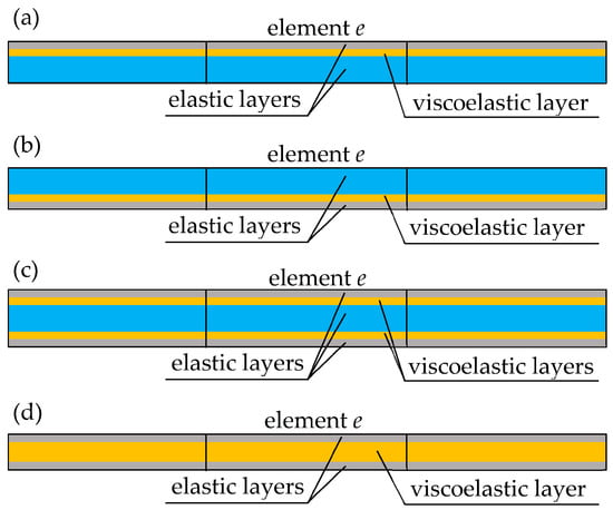
Figure 1.
Multilayered elements: (a) elastic core laminated on the top, (b) elastic core laminated on the bottom, (c) elastic core laminated on both sides, and (d) sandwich element.
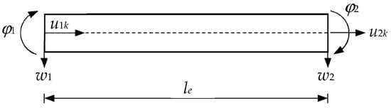
Figure 2.
kth layer of element e (modeled as a beam finite element).
2.1. Elastic Layers
According to the Euler–Bernoulli theory, the cross-section of a layer is infinitely rigid. It remains plane after deformation and perpendicular to the beam deformation axis.
If is the horizontal displacement in the center of the kth elastic layer, w is the vertical displacement, and θ is the angle between a normal to the cross-section before and after deformation , the displacement field of the kth elastic layer is expressed as follows:
where and is vector of nodal displacements. denotes matrix of shape functions:
where . Horizontal displacements are approximated using linear functions, whereas vertical ones are approximated using Hermite polynomials.
Hence, the generalized strain vector can be written in terms of nodal displacements in the following form:
where , is the axial strain of the kth layer , κ is the curvature , and matrix can be expressed as follows:
2.2. Viscoelastic Layer
The Timoshenko theory was used to model the viscoelastic layer. Based on this theory, the horizontal displacement of the viscoelastic layer is expressed by the horizontal displacements of the constraining elastic layers (Figure 3). Effects of shear deformation are taken into account, and the angle of rotation of the cross-section is defined as follows:
where is the angle of rotation after deformation and is the averaged angle of rotation.
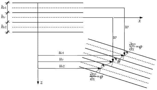
Figure 3.
Deformation of viscoelastic layer.
The displacement field is described as follows:
where and ,
, , and hv denotes the height of the viscoelastic layer. Indexes e1 and e2 refer to the upper and lower elastic layers, respectively (see Figure 3).
The generalized strain vector for the viscoelastic layer can be expressed as follows:
where , and κ is the curvature of the Timoshenko layer defined as Matrix Bk is expressed as follows:
2.3. Matrix Formulation of Equation of Motion for Composite Beam
Matrices for kth layer can be determined using the virtual work principle. Matrix for kth layer is expressed as follows:
where is the mass per unit length of layer, is the mass moment of inertia, and can be calculated using Equation (2) or Equation (7) for the kth elastic layer and the kth viscoelastic layer, respectively. Stiffness matrix for the kth elastic layer is expressed as follows:
where is Young’s modulus, is the moment of inertia of the layer’s cross-section, and can be calculated using Equation (4). Stiffness matrices for the kth viscoelastic layer can be computed using the following expressions:
where , is the relaxed elastic modulus, is the nonrelaxed elastic modulus, , , v is the Poisson ratio, d is the shear factor, and can be calculated using Equation (9). Based on these formulas, elemental matrices can be assembled.
The equation of motion of the composite beam with viscoelastic layers can be written as follows:
where and are the Laplace transforms of global vectors of displacements and excitation forces, respectively, and s is the Laplace variable. M, K, and Kv(s) are global matrices built on the basis of elemental mass matrix , elemental stiffness matrix , and elemental matrix :
where nr is the number of viscoelastic layers of the finite element under consideration.
2.4. Dynamic Characteristics of Composite Beam
After assuming , the following nonlinear eigenproblem is obtained:
Eigenvalues and eigenvectors are solutions to the eigenproblem (16), which can be determined using the continuation method [35,36] or the subspace iteration method [37]. In this study, natural frequency and the nondimensional damping ratio were analyzed. The dynamic characteristics can be calculated as follows:
if eigenvalue is written as , .
3. Uncertain Design Parameters
3.1. Interval Analysis
Moore [5] presented the fundamentals of interval analysis. Any parameter pi can be described as an interval number as follows:
This means that it can vary within certain limits, where is the lower bound and is the upper bound. The middle value of the interval parameter can be expressed as follows:
and the radius value is determined as follows:
Operations on interval numbers require calculations that consider all possible combinations of upper and lower limits of the considered quantities. The result is the interval whose bounds are the smallest and largest result values. The basic operations on sample interval numbers and are calculated as follows:
The major problem of the application of direct interval analysis to engineering problems is the huge overestimation of obtained results. This is because each interval number is treated as an independent variable even if it represents the same physical quantity. Nevertheless, interval analysis is a highly useful tool for obtaining responses of structures with parameters whose values change within certain limits. However, the overestimation that may be present in the obtained limits of the solutions needs to be eliminated.
3.2. Approximation of the Lower and Upper Bounds of Objective Function Based on Taylor Series Expansion
Uncertainties of design parameters whose limits are known can be taken into account using the Taylor series expansion of the objective function in the vicinity of the middle values of parameters. The objective function is the response function of the structure denoted as , where is a set of interval design parameters. It can be expressed as follows:
where is the lower bound of function and is the upper bound of function . In this study, the objective function is the dynamic characteristics of a composite beam with viscoelastic layers; however, the presented approach is general, and the objective function can be any quantity related to the response of the structure.
The lower and upper bounds of the objective function can be calculated by Taylor series expansion using the first two elements of this series:
where is the value of the response function for the values of the middle parameters and is the first-order derivative of the response function with respect to parameter pi (the so-called sensitivity of the first order with respect to the change of design parameter pi). The function f(p) is the new value of the response function containing the effect of the changing parameter pi, which can be rewritten as follows:
where the second term of Equation (27) is the increment in the response function:
Hence the response of structures with uncertain parameters can be expressed as follows:
where the lower and upper bounds of the increment can be written as follows:
It is assumed that design parameters take the values at the edges of the intervals and that parameters vary independently. The maximum and minimum values of the increment ( and ) are determined after considering all possible combinations of . The increment in the interval parameter means that two possible increments in the parameter i are taken into account in the calculations:
The number of combinations needed to consider for selecting the smallest and largest values of the increments is 2r. However, when the number of parameters or their variability is high, the approximation of the limits of the objective function using a first-order Taylor series expansion may be insufficient.
If a higher accuracy is required, an approximation using the first three terms of the Taylor series can be used (second-order Taylor series expansion):
where is the second-order derivative with respect to parameters pi and pj (the so-called sensitivity of the second order with respect to the simultaneous change in two design parameters pi and pj). Derivatives of the second order form the following Hessian matrix:
In this case, increments in Equation (27) can be written as follows:
where the increment for parameter i can be expressed as follows:
To find the minimum or maximum values of the increment , it is necessary to consider combinations. With a high number of parameters, this method is laborious and inefficient. The number of combinations can be reduced by eliminating nondiagonal elements of the Hessian matrix [23], which can be expressed as follows:
In this case, the effect of the simultaneous change in design parameters is not taken into account and Equation (34) can be written as follows:
Therefore, the number of combinations is the same as in the case of applying the first two elements of the Taylor series for calculations, but it requires second-order sensitivity calculations. Sensitivity is calculated according to the algorithm presented in [38] which was used for beams with viscoelastic layers in [39,40].
3.3. Vertex Method
In the vertex method, design parameters are assumed to be interval values. In this method, all possible combinations of lower and upper parameter bounds are investigated, and then, the smallest and largest values of the response function are selected. The values obtained this way are close to the exact solution, and this method can be used as a comparative method. The number of combinations to be considered is .
4. Algorithm for Determining Critical Combinations of Parameters
Due to the large number of combinations required, the vertex method is not effective, but the combination of parameters obtained using this method allows one to calculate the bounds of the objective function. Using Taylor series expansion does not always result in determining the same combination of parameters as in the vertex method, especially if uncertainties are large. The algorithm presented below uses the Taylor series expansion, but even in the case of a large number of parameters or their variability, it gives exactly the same combination of parameter values as the vertex method. In [25], this algorithm was used to analyze structures with viscoelastic dampers; however, in this study, it is proved that this algorithm is general and can be used for other structures with viscoelastic damping elements. In addition, this algorithm is more efficient than the vertex method.
In the first step, the first- and second-order sensitivities with respect to the change in each design parameter, which was assumed as an interval value, are calculated. Then, according to Equation (37), increments in the limit values of design parameters are performed, and the largest among them is selected. In the second step, the value of the parameter with the largest is updated, and first- and second-order sensitivities are recalculated with respect to the change in design parameters. The parameter whose value was set in the previous step is not taken into further consideration. As mentioned earlier, the largest increment is selected, and the appropriate parameter value is updated. The calculations are repeated until the limit values of all parameters are determined. In the last step, the upper bound of the objective function for the set parameter values is calculated. The same analysis is conducted to determine the parameter values, thus allowing the calculation of the lower bound of the objective function. The analyzed examples show that this algorithm allows one to determine the same critical combination of limit values of parameters as the vertex method, but it is less labor intensive. The pseudocode for the presented algorithm is as follows (see Algorithm 1):
| Algorithm 1: Determining the critical combination of parameters. |
| 1° Input data: r—number of uncertain parameters —vector of lower bounds of uncertain parameters —vector of upper bounds of uncertain parameters —vector of middle values of uncertain parameters 2° set n:= r set ( denotes parameter vector for the critical combination) 3° for i = 1,2,…,n calculate sensitivities of the response function with respect to change in parameter (sensitivities of the first order) and (sensitivities of the second order) 4° for i = 1,2,…,n calculate the increment in response function according to Equation (37) for and 5° select the maximum value of and corresponding parameter 6° substitute 7° exclude parameter and its lower and upper bounds from futher calculations 8° update n:=n − 1 9° repeat steps 3° to 8° until n = 0 10° calculate the maximum value of the response function for the critical combination of parameters . |
To find the lower bound of the structure response and corresponding parameters, the above algorithm is repeated, but in step 5°, the minimum value of has to be selected (.
A flowchart of the algorithm for determining the critical combination of parameters for the upper bound of the structure response is shown in Figure 4. To find the lower bound, the minimum value of and the corresponding parameter pk must be selected.
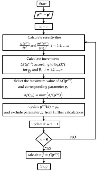
Figure 4.
Flowchart for determining the critical combination of parameters.
5. Examples
A composite five-layered beam is analyzed with the arrangement of layers shown in Figure 5. Elastic layers are described by the following parameters: and . Viscoelastic layers are described as follows: , , and The Poisson ratio is , the relaxation time is , and the fractional order is . The heights of the layers are as follows (notation as presented in Figure 4): , , , , and . The length of the beam is 0.2 m, and the calculations are carried out by dividing the beam into 10 elements. Various boundary conditions are considered.
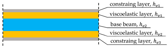
Figure 5.
Scheme of the considered five-layered composite beam.
Calculations are made using codes written in Matlab.
5.1. Veryfication Example
To verify the correctness of the performed calculations, the natural frequencies and nondimensional damping ratios were computed for the simply supported sandwich beam considered in [35] (Figure 6). The heights of the elastic and the viscoelastic layers are as follows: , , and . The remaining parameters are the same as described above. Table 2 presents the first four natural frequencies and nondimensional damping ratios. The maximum difference for the fourth natural frequency is 0.017%. The obtained results confirm the correctness of the obtained dynamic characteristics for the considered beam.
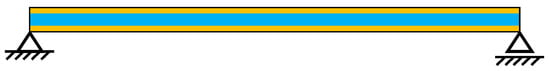
Figure 6.
Scheme of the sandwich beam considered in [35].
Table 2.
Comparison of natural frequencies of a sandwich beam.
5.2. The Influence of the Layer Height Uncertainty
Four types of boundary conditions were considered, as shown in Figure 7. The first natural frequency ω1 and the first nondimensional damping ratio γ1 were analyzed. The central parameter values are presented in Table 3.
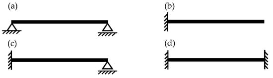
Figure 7.
Scheme of the considered five-layered composite beam (a) simply supported, (b) cantilever, (c) fixed-pinned and (d) fixed-fixed.
Table 3.
Natural frequencies and nondimensional damping ratio for different boundary conditions.
It is assumed that layer heights are uncertain parameters and can be varied independently. Uncertainties from 5% to 30% with 5% steps are considered. The interval values of the parameters for the smallest and the largest considered uncertainties are presented in Table 4.
Table 4.
Interval values of uncertain parameters he and hv.
In Figure 8, Figure 9, Figure 10 and Figure 11, the ranges of natural frequencies and nondimensional damping ratios for different boundary conditions are presented. Final values are calculated using the vertex method (Method I—black line), the first-order Taylor series expansion (Method II—blue line), the second-order Taylor series expansion with only diagonal elements of the Hessian matrix (Method III—red line), and the second-order Taylor series expansion with all components of the Hessian matrix (Method IV—green line).
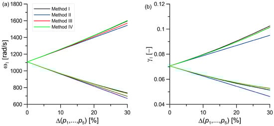
Figure 8.
Ranges of interval values of (a) natural frequency ω1 and (b) nondimensional damping ratio γ1 for a simply supported beam.
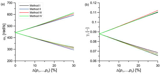
Figure 9.
Ranges of interval values of (a) natural frequency ω1 and (b) nondimensional damping ratio γ1 for a cantilever beam.
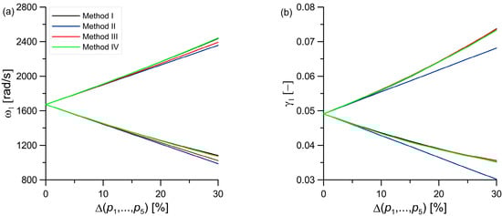
Figure 10.
Ranges of interval values of (a) natural frequency ω1 and (b) nondimensional damping ratio γ1 for a fixed-pinned beam.
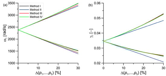
Figure 11.
Ranges of interval values of (a) natural frequency ω1 and (b) nondimensional damping ratio γ1 for a fixed-fixed beam.
In all cases, as shown in the graphs for variations up to 10%, the results from all four methods are very close and the lines in the graphs almost overlap. This applies to both the natural frequency and the nondimensional damping ratio for all considered boundary conditions. This confirms that even the simplest method of predicting a solution for uncertain design parameters (a first-order Taylor series expansion) is sufficient to achieve good results.
When large uncertainties are considered, in the case of natural frequency, the second-order Taylor series expansion with all components of the Hessian matrix provides results closest to the vertex method. However, it is relatively time consuming due to the number of combinations required. In the case of the nondimensional damping ratio, this method usually gives results closest to the vertex method, but the discrepancies are larger and, in some cases, a smaller range of results is obtained (i.e., the lower limit for simply supported or fixed-fixed beams) than using the vertex method. In this case, the solution does not take into account all cases that may occur.
For this reason, it seems to be important to determine the same critical combination of design parameters as in the case of the vertex method. Therefore, the algorithm presented in Section 4 (Method V) was used. In Table 5 and Table 6, the results for a simply supported beam with the uncertainty of design parameters equal to 10% and 30% are presented.
Table 5.
Lower and upper bounds of natural frequency ω1 for a simply supported beam with uncertain design parameters equaling 10%.
Table 6.
Lower and upper bounds of natural frequency ω1 for a simply supported beam with uncertain design parameters equaling 30%.
Based on the results presented in Table 5 and Table 6, it can be concluded that Method V yields the same critical combination of design parameters and the same results as the vertex method. In addition, it is more efficient than Method IV, as described in Section 5.4.
5.3. The Influence of the Parameters and of the Viscoelastic Layers
It is assumed that the parameters describing the viscoelastic layers E0v1, E0v2, E∞v1, and E∞v2 are uncertain parameters. The first two natural frequencies and nondimensional damping ratios were analyzed for the simply supported beam. It is assumed that the parameter uncertainties change from 5% to 30% with 5% steps. In Table 7, parameter values for the smallest and largest uncertainties are presented.
Table 7.
Interval values of uncertain parameters E0 and E∞.
In Figure 10 and Figure 11, the lower and upper limits of the dynamic characteristics with respect to the change in the uncertainties of the E0 and E∞ are presented. The calculations, as discussed in Section 5.2, are performed using four methods.
The graphs presented in Figure 12 and Figure 13 show that for E0 and E∞ of the viscoelastic layers, all four methods give similar results, as well as for the higher mode. In this case, the calculation of the first-order sensitivity is therefore quite sufficient to predict the behavior of the structure.
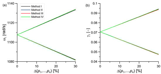
Figure 12.
Ranges of interval values of (a) natural frequency ω1 and (b) nondimensional damping ratio γ1.
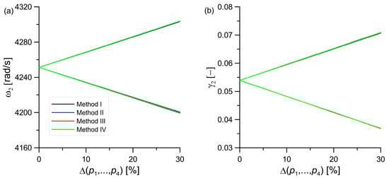
Figure 13.
Ranges of interval values of (a) natural frequency ω2 and (b) nondimensional damping ratio γ2.
5.4. The Influence of the Parameters α and τ of the Viscoelastic Layers
In the third example, it is assumed that the parameters α and τ are uncertain. The first four natural frequencies for a simply supported beam are analyzed. It is assumed that the parameters change simultaneously for both viscoelastic layers, i.e., the number of changing parameters is two. Due to the high influence of α on the structure response, it was assumed that the uncertainty of this parameter is constant and amounts to 5%, whereas the uncertainties of τ change from 5 % to 30% with 5% step. The interval values of α and for the smallest and largest parameter τ are shown in Table 8.
Table 8.
Interval values of uncertain parameters α and τ.
In Figure 14, a comparison of natural frequencies calculated using four methods is presented. The collapse of the graphs for 5% is because the uncertainty of α is constant and is equal to 5%, whereas only the uncertainty of τ changes.
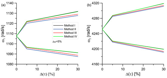
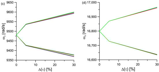
Figure 14.
Ranges of interval values of first four natural frequencies for (a) 1st natural frequency, (b) 2nd natural frequency, (c) 3rd natural frequency and (d) 4th natural frequency.
To check the effects of the uncertainty of α on the natural frequencies, the lower and upper limits for the uncertainty of α of 5%, 15%, and 25% are shown on the same graph. Because Method IV gives results similar to those of the vertex method (see Figure 14), only these two methods are presented in Figure 15.
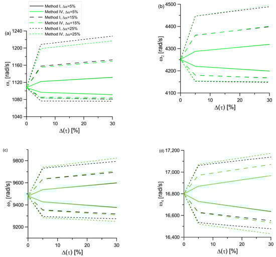
Figure 15.
Ranges of interval values of first four natural frequencies for different changes of α (a) 1st natural frequencies, (b) 2nd natural frequencies, (c) 3rd natural frequencies and (d) 4th natural frequencies.
The effect of the uncertainty of α is quite significant. The graphs show that with an increase in the uncertainty of the parameter, the solutions obtained using the vertex method, and Method IV differ already for uncertainties of 5%. Hence, it is reasonable to use the method described in Section 4. In Table 9, Table 10, Table 11 and Table 12, the results for four selected cases of uncertainties are presented.
Table 9.
Lower and upper bounds of natural frequency ω1 for a simply supported beam and uncertainty of design parameters and .
Table 10.
Lower and upper bounds of natural frequency ω1 for a simply supported beam and uncertainty of design parameters and .
Table 11.
Lower and upper bounds of natural frequency ω1 for a simply supported beam and uncertainty of design parameters and .
Table 12.
Lower and upper bounds of natural frequency ω1 for a simply supported beam and uncertainty of design parameters and .
5.5. Comparison of Methods
In Table 13, the number of combinations that should be considered in order to select the largest or smallest increment in the objective function is presented, and the number of eigenproblems to be solved for the given design parameters is analyzed.
Table 13.
Comparison of the methods.
Methods I and V always result in the same critical combination of parameters, and Method V is effective also for large uncertainties. The number of combinations is smaller for method V if the number of parameters is higher than four, and the number of tasks to be solved is smaller for two parameters. In addition, Methods II and III are comparable in terms of the number of combinations and the number of tasks to be solved, but in the case of high uncertainties, they provide results that differ from those of the vertex method. Method IV gives results similar to the vertex method, as well as for large uncertainties, but the critical combination of parameters obtained is not always the same as in the case of the vertex method. Hence, for large uncertainties, Method V is recommended.
6. Conclusions
This study presents an analysis of a composite beam with viscoelastic layers, assuming that design parameters are uncertain. The exact value of the parameter is unknown, but the bounds of the parameters are known. Hence, interval calculus can be used. The most common method, but also the most laborious, due to the number of combinations that need to be performed, is the vertex method. This study proposes four different methods based on expanding the objective function into a Taylor series.
The conducted analyses aimed to determine which of the presented methods would be the most beneficial for determining the dynamic characteristics of a composite beam with viscoelastic layers. However, the choice of method depends on the number of uncertain parameters and the value of the parameter uncertainty. If there are a small number of parameters and small uncertainties, the method that uses the first-order Taylor series expansion can be successfully applied. With large uncertainties and a larger number of parameters, Method V is recommended. The presented examples confirm that it yields good results and is not laborious.
Funding
This research was funded by the research project of Poznan University of Technology, grant number 0411/SBAD/0008.
Institutional Review Board Statement
Not applicable.
Informed Consent Statement
Not applicable.
Data Availability Statement
The data presented in this article and used codes are available upon request to the corresponding author.
Conflicts of Interest
The author declares no conflict of interest.
References
- Fishman, G.S. Monte Carlo: Concepts, Algorithms and Applications; Springer-Verlag: Berlin, Germany, 1996. [Google Scholar]
- Kleiber, M.; Hien, H.D. The Stochastic Finite Element Method: Basic Perturbation Technique and Computer Implementation; John-Wiley & Sons: Chichester, UK, 1992. [Google Scholar]
- Ghanem, R.G.; Spanos, P.D. Stochastic Finite Elements: A Spectral Approach; Springer: New York, NY, USA, 1991. [Google Scholar]
- Elishakoff, I.; Ohsaki, M. Optimization and Anti-Optimization of Structures under Uncertainties; Imperial College Press: London, UK, 2010. [Google Scholar]
- Moore, R.E. Methods and Applications of Interval Analysis; Prentice Hall: London, UK, 1979. [Google Scholar]
- Dimarogonas, A.D. Interval analysis of vibrating systems. J. Sound Vib. 1995, 183, 739–749. [Google Scholar] [CrossRef]
- Yang, X. Interval finite element based on the element for eigenvalue analysis of structures with interval parameters. Struct. Eng. Mech. 2001, 12, 669–684. [Google Scholar] [CrossRef]
- Chen, S.H.; Lian, H.D.; Yang, W.Y. Interval eigenvalue analysis for structures with interval parameters. Finite Elem. Anal. Des. 2003, 39, 419–431. [Google Scholar] [CrossRef]
- Chen, S.H.; Lian, H.D. Dynamic response analysis for structures with interval parameters. Struct. Eng. Mech. 2002, 13, 299–312. [Google Scholar] [CrossRef]
- Qiu, Z.; Wang, X. Parameter perturbation method for dynamic responses of structures with uncertain-but-bounded parameters based on interval analysis. Int. J. Solids Struct. 2005, 42, 4958–4970. [Google Scholar] [CrossRef]
- Sim, J.; Qiu, Z.; Wang, X. Modal analysis of structures with uncertain-but-bounded parameters via interval analysis. J. Sound Vib. 2007, 303, 29–45. [Google Scholar] [CrossRef]
- Qiu, Z.; Wang, X. Vertex solution theorem for the upper and lower bounds on the dynamic response of structures with uncertain-but-bounded parameters. Acta Mech. Sin. 2009, 25, 367–379. [Google Scholar] [CrossRef]
- Qiu, Z.; Wang, P. Parameter vertex method and its parallel solution for evaluating the dynamic response bounds of structures with interval parameters. Sci. China Phys. Mech. Astron. 2018, 61, 064612. [Google Scholar] [CrossRef]
- Madares, M.; Asce, M.; Mullen, R.L.; Asce, F.; Muhanna, R.L.; Asce, M. Natural frequencies of a structure with bounded uncertainty. J. Eng. Mech. 2006, 132, 1363–1371. [Google Scholar] [CrossRef]
- Yaowen, Y.; Zhenhan, C.; Yu, L. Interval analysis of frequency response functions of structures with uncertain parameters. Mech. Res. Commun. 2013, 47, 24–31. [Google Scholar] [CrossRef]
- Yaowen, Y.; Zhenhan, C.; Yu, L. Interval analysis of dynamic response of structures using Laplace transform. Probabilistic Eng. Mech. 2012, 29, 32–39. [Google Scholar]
- Muscolino, G.; Santoro, R.; Sofi, A. Explicit frequency response functions of discretized structures with uncertain parameters. Comput. Struct. 2014, 133, 64–78. [Google Scholar] [CrossRef]
- Feng, X.; Wu, J.; Zhang, Y. Time response of structure with interval and random parameters using a new hybrid uncertain analysis method. Appl. Math. Model. 2018, 64, 426–452. [Google Scholar] [CrossRef]
- Li, Q.; Han, J.; Yang, J.; Guo, X. The exact extreme response and the confidence extreme response analysis of structures subjected to uncertain-but-bounded excitations. Appl. Math. Model. 2020, 77, 1742–1761. [Google Scholar] [CrossRef]
- Qiu, Z.; Ni, Z. Interval modal superposition method for impulsive response of structures with uncertain-but-bounded external loads. Appl. Math. Model. 2011, 35, 1538–1550. [Google Scholar] [CrossRef]
- Wei, T.; Li, F.; Meng, G. A bivariate Chebyshev polynomials method for nonlinear dynamic systems with interval uncertainties. Nonlinear Dyn. 2022, 107, 793–811. [Google Scholar] [CrossRef]
- Qiu, Z.; Ma, L.; Wang, X. Non-probabilistic interval analysis method for dynamic response analysis of nonlinear systems with uncertainty. J. Sound Vib. 2009, 319, 531–540. [Google Scholar] [CrossRef]
- Chen, S.H.; Ma, L.; Meng, G.W.; Guo, R. An efficient method for evaluating the natural frequencies of structures with uncertain-but-bounded parameters. Comput. Struct. 2009, 87, 582–590. [Google Scholar] [CrossRef]
- Fujita, K.; Takewaki, I. An efficient methodology for robustness evaluation by advanced interval analysis using updated second-order Taylor series expansion. Eng. Struct. 2011, 33, 3299–3310. [Google Scholar] [CrossRef]
- Łasecka-Plura, M.; Lewandowski, R. Dynamic characteristics and frequency response function for frame with dampers with uncertain design parameters. Mech. Based Des. Struct. Mach. 2017, 45, 296–312. [Google Scholar] [CrossRef]
- Kamiński, M.; Lenartowicz, A.; Guminiak, M.; Przychodzki, M. Selected problems of random free vibrations of rectangular thin plates with viscoelastic dampres. Materials 2022, 15, 6811. [Google Scholar] [CrossRef]
- Muscolino, G.; Sofi, A. Stochastic analysis of structures with uncertain-but-bounded parameters via improved interval analysis. Probabilistic Eng. Mech. 2012, 28, 152–163. [Google Scholar] [CrossRef]
- Wang, C.; Gao, W.; Song, C.; Zhang, N. Stochastic interval analysis of natural frequency and mode shape of structures with uncertainties. J. Sound Vib. 2014, 333, 2483–2503. [Google Scholar] [CrossRef]
- Tian, W.; Chen, W.; Ni, B.; Jiang, C. A single-loop method for reliability-based design optimization with interval distribution parameters. Comput. Methods Appl. Mech. Eng. 2022, 391, 114372. [Google Scholar] [CrossRef]
- Jiang, C.; Han, X.; Guan, F.J.; Li, Y.H. An uncertain structural optimization method based on nonlinear interval number programming and interval analysis method. Eng. Struct. 2007, 29, 3168–3177. [Google Scholar] [CrossRef]
- Meggitt, J.W.R. Interval-based identification of response-critical joints: A tool for model refinement. J. Sound Vib. 2022, 529, 116850. [Google Scholar] [CrossRef]
- Wang, L.; Wang, X.; Li, Y.; Lin, G.; Qiu, Z. Structural time-dependent reliability assessment of the vibration active control system with unknown-but-bounded uncertainties. Struct. Control. Health Monit. 2017, 24, e1965. [Google Scholar] [CrossRef]
- Hernandez, W.P.; Castello, D.A.; Ritto, T.G. Uncertainty propagation analysis in laminated structures with viscoelastic core. Comput. Struct. 2016, 164, 23–37. [Google Scholar] [CrossRef]
- Galucio, A.C.; Deu, J.F.; Ohayon, R. Finite element formulation of viscoelastic sandwich beams using fractional derivative operators. Comput. Mech. 2004, 33, 282–291. [Google Scholar] [CrossRef]
- Lewandowski, R.; Baum, M. Dynamic characteristics of multilayered beams with viscoelastic layers described by the fractional Zener model. Arch. Appl. Mech. 2015, 85, 1793–1814. [Google Scholar] [CrossRef]
- Pawlak, Z.; Lewandowski, R. The continuation method for the eigenvalue problem of structures with viscoelastic dampers. Comput. Struct. 2013, 125, 53–61. [Google Scholar] [CrossRef]
- Łasecka-Plura, M.; Lewandowski, R. The subspace iteration method for nonlinear eigenvalue problems occurring in the dynamics of structures with viscoelastic elements. Comput. Struct. 2021, 254, 106571. [Google Scholar] [CrossRef]
- Lewandowski, R.; Łasecka-Plura, M. Design sensitivity analysis of structures with viscoelastic dampers. Comput. Struct. 2016, 164, 95–107. [Google Scholar] [CrossRef]
- Łasecka-Plura, M.; Lewandowski, R. Sensitivity analysis of dynamic characteristics of composite beams with viscoelastic layers. Procedia Eng. 2017, 199, 366–371. [Google Scholar] [CrossRef]
- Łasecka-Plura, M. A comparative study of the sensitivity analysis for systems with viscoelastic elements. Arch. Mech. Eng. 2023, 70, 5–25. [Google Scholar]


Disclaimer/Publisher’s Note: The statements, opinions and data contained in all publications are solely those of the individual author(s) and contributor(s) and not of MDPI and/or the editor(s). MDPI and/or the editor(s) disclaim responsibility for any injury to people or property resulting from any ideas, methods, instructions or products referred to in the content. |
© 2023 by the author. Licensee MDPI, Basel, Switzerland. This article is an open access article distributed under the terms and conditions of the Creative Commons Attribution (CC BY) license (https://creativecommons.org/licenses/by/4.0/).