Spatiotemporal Matching Cost Function Based on Differential Evolutionary Algorithm for Random Speckle 3D Reconstruction

Abstract

Random speckle structured light can increase the texture information of the object surface, so it is added in the binocular stereo vision system to solve the matching ambiguity problem caused by the surface with repetitive pattern or no texture. To improve the reconstruction quality, many current researches utilize multiple speckle patterns for projection and use stereo matching methods based on spatiotemporal correlation. This paper presents a novel random speckle 3D reconstruction scheme, in which multiple speckle patterns are used and a weighted-fusion-based spatiotemporal matching cost function (STMCF) is proposed to find the corresponding points in speckle stereo image pairs. Furthermore, a parameter optimization method based on differential evolutionary (DE) algorithm is designed for automatically determining the values of all parameters included in STMCF. In this method, since there is no suitable training data with ground truth, we explore a training strategy where a passive stereo vision dataset with ground truth is used as training data and then apply the learned parameter value to the stereo matching of speckle stereo image pairs. Various experimental results verify that our scheme can realize accurate and high-quality 3D reconstruction efficiently and the proposed STMCF exhibits superior performance in terms of accuracy, computation time and reconstruction quality than the state-of-the-art method based on spatiotemporal correlation.

1. Introduction

Three-dimensional reconstruction technique based on measurement has been widely applied in various fields, such as industrial manufacturing [1], protection of historical relics [2], architectural design [3], digital entertainment [4], etc. It is an active and important research direction in the field of computer vision. The key point of this technique is how to acquire the depth information of the measured object. At present, measurement-based 3D reconstruction methods can be mainly divided into two classes: passive and active measurement methods.

The passive measurement methods generally obtain images by cameras from multi-views, then 3D spatial information of the measured object is calculated by a specific algorithm. Among them, binocular stereo vision is one of the most widely used methods due to low cost and being easy for implementation. It firstly finds the corresponding points between stereo image pairs captured by two cameras from different views and then the depth information is recovered by triangulation. Stereo matching is a critical and challenging work of binocular stereo vision, which determines the correctness of corresponding points and the accuracy of depth information. Many kinds of stereo matching algorithms have been proposed by researchers in the last decades [5,6,7,8,9,10]. However, there is still no good solution for repetitive pattern and textureless regions.

The active measurement methods usually emit optical signals to the surface of the object. Both time of flight (TOF) [11] and structured light [12] are typical active approaches. The TOF camera transmits continuous near-infrared ray to the target, then the reflected ray is received by a specific sensor. By measuring the flight time of the ray, the depth information is obtained. It has advantages of fast response and less computational cost. Nevertheless, it has the shortcomings of low accuracy and depth map resolution.

The structured light technique also works on the principle of triangulation. Different with passive binocular stereo vision, it improves 3D reconstruction quality by projecting a pre-designed pattern onto the object. Fringe structured light [13] and random speckle structured light [14] are two mainstream structured light encoding methods currently. Compared with the former, random speckle structured light does not need accurate phase shift and the cost of projection equipment is relatively low. Hence, it is widely applied in various commercial 3D sensors, such as Kinect [4], RealSense [15], etc. As shown in Figure 1 (the photo in Figure 1 is a plastic human face mask, as are photos in Figure 2), random speckle structured light is commonly used in combination with the binocular stereo vision system because it can enrich texture information of the object surface that is helpful to find the matching point more accurately. In order to improve the reconstruction quality, many existing studies utilize multiple speckle patterns for projection and use stereo matching methods based on spatiotemporal correlation.

Figure 1. Schematic of binocular stereo vision system using random speckle structured light.

Figure 2. Schematic diagram of the proposed random speckle 3D reconstruction scheme.

In this paper, a novel random speckle 3D reconstruction scheme is presented. Sequence of different speckle patterns are projected to the measured object and then two cameras capture images from different views synchronously. The speckle pattern that we used is designed by [16]. After acquiring sequence of speckle image pairs, the schematic diagram of the scheme is shown in Figure 2 and the main contributions are as follows:

(1)

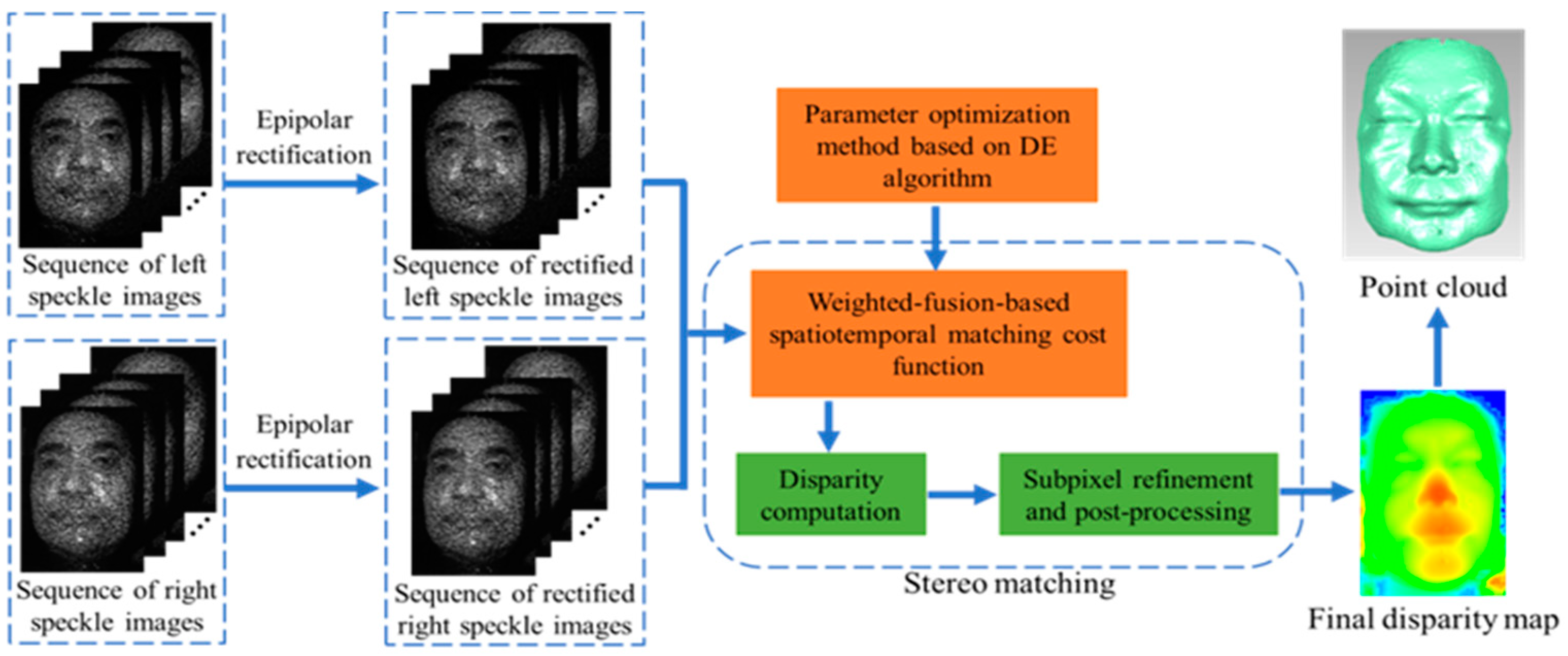
A weighted-fusion-based spatiotemporal matching cost function (STMCF) is proposed for accurately searching the matching point pairs between left and right speckle images.

(2)

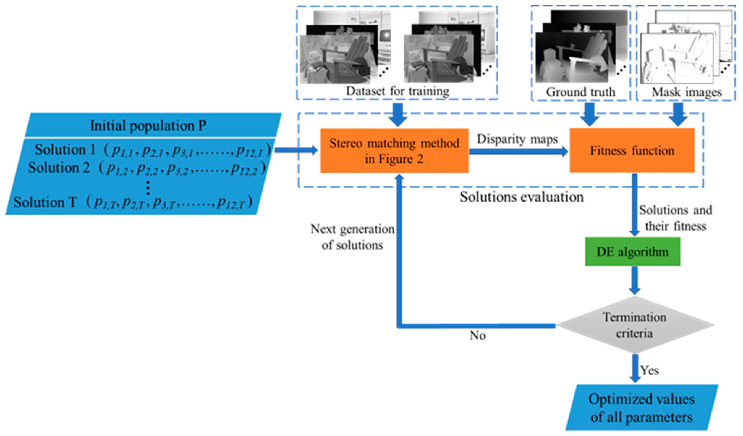
In order to automatically determine the value of each parameter used in STMCF, a parameter optimization method based on differential evolutionary (DE) algorithm is designed and a training strategy is explored in this method.

(3)

A series of comparative experimental results indicate that our scheme can achieve accurate and high-quality 3D reconstruction efficiently and the proposed STMCF can provide better performance on the aspects of accuracy, computation time and reconstruction quality than the state-of-the-art method based on spatiotemporal correlation, which is widely used in random speckle 3D reconstruction.

The remainder of this paper is organized as follows. The related work is discussed in Section 2. Section 3 describes the STMCF. Disparity computation and subpixel refinement are given in Section 4. The parameter optimization method based on DE algorithm is presented in Section 5. Experiments and discussion are provided in Section 6 and finally, Section 7 concludes this paper.

2. Related Works

2.1. Weighted-Fusion-Based Matching Cost Function

The main task of matching cost function is to quantify the matching cost of corresponding points between stereo image pairs. Classical matching cost computation methods can be divided into three kinds: pixel-based methods, window-based methods and non-parametric methods. Each kind of method has their own disadvantages. Hence, the commonly used form of matching cost function is the weighted-fusion of several different methods.

Mei et al. [17] effectively combined the absolute differences (AD) and Census transformation [18], known as AD-Census. It provided more accurate matching result than individual method. Hosni et al. [19] used the pixel-based truncated absolute difference of AD and gradient as the matching cost, which was robust to illumination changes. Hamzah et al. [20] proposed a new matching cost function that combined three different similarity measures including AD, gradient and Census transformation. It could reduce the radiometric distortions and the effect of illumination variations. More recently, Hong et al. [21] proposed a weighted-fusion matching cost function that included AD, square difference (SD), Census and Rank transformations. In addition, they considered the stereo matching as an optimization problem and used an evolutionary algorithm to automatically optimize the parameters in the cost function.

The mentioned above weighted-fusion-based matching cost functions were all designed for passive binocular stereo vision, so they only considered the spatial feature and could not utilize the temporal feature brought by multiple speckle stereo image pairs.

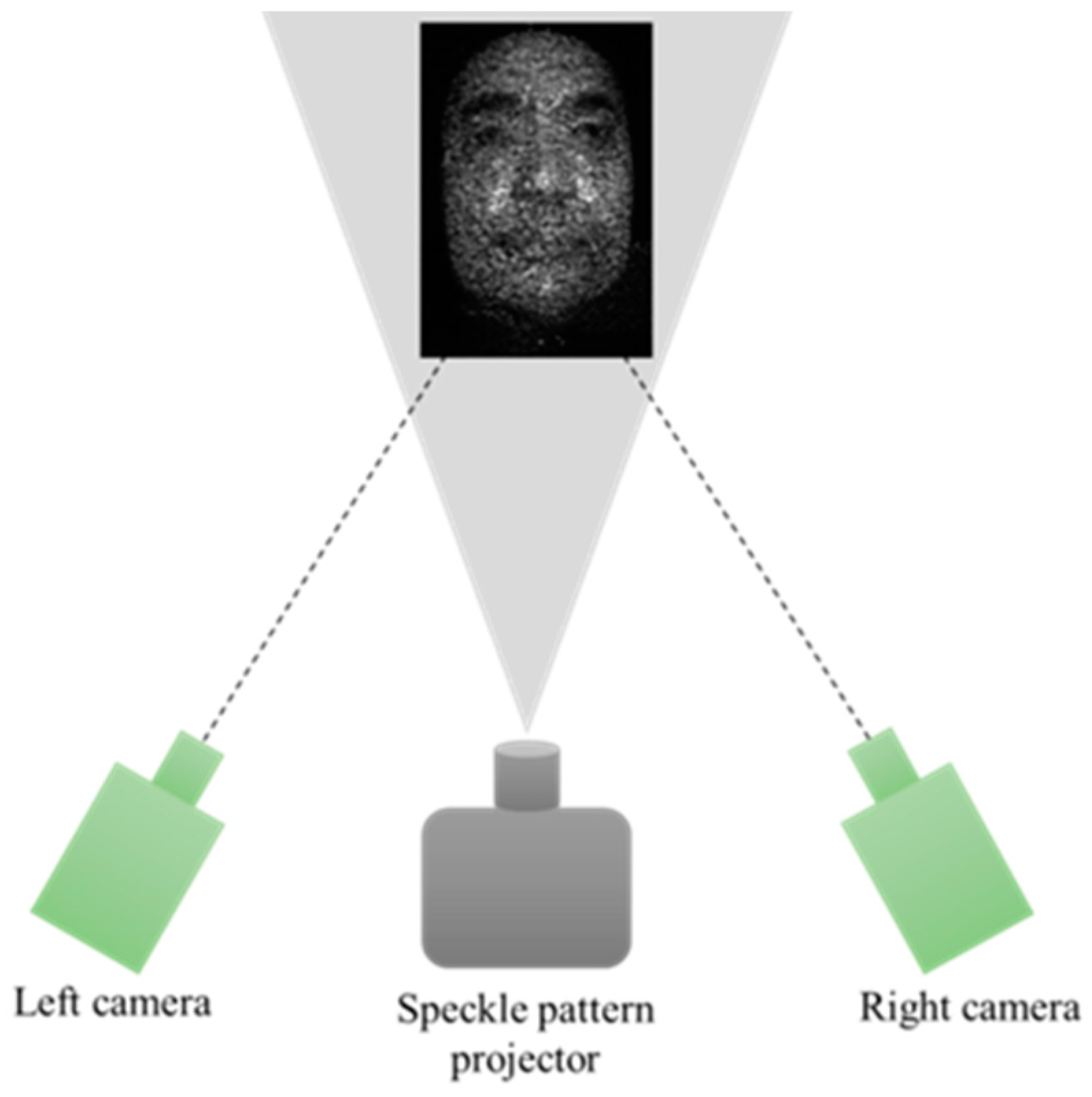
2.2. 3D Reconstruction Based on Binocular Stereo Vision with Random Speckle Projection

Since random speckle structured light can effectively improve the accuracy of stereo matching, a lot of research on 3D reconstruction based on binocular stereo vision with random speckle projection has been reported. According to the number of projected patterns, they can be mainly classified into two types.

The first type used the single speckle pattern. Gu et al. [22] proposed an improved semi-global matching algorithm using the single-shot random speckle structured light. In this algorithm, a new penalty term was defined for alleviating the ladder phenomenon. Although it could achieve 3D dynamic reconstruction, the measurement accuracy was relatively low. Yin et al. [23] designed an end-to-end stereo matching network for single-shot 3D shape measurement. It firstly used a multi-scale residual sub-network to extract feature tensors from speckle images, then a lightweight 3D U-net network was proposed to implement efficient cost aggregation. Zhou et al. [14] presented a high-precision 3D measurement scheme that used a single-shot color binary speckle pattern and an extended temporal-spatial correlation matching algorithm for the measurement of dynamic and static objects. However, when the object surface is colorful, the measurement effect may be affected.

The second type used multiple different speckle patterns. To acquire high-quality results, many current studies employ stereo matching methods based on spatiotemporal correlation. Tang et al. [24] proposed an improved 3D reconstruction method through combining advantages of both spatial correlation and temporal correlation methods. Meanwhile, by analyzing the relationship between the correlation window size and the number of speckle patterns, the tradeoff between the accuracy and efficiency was found. Fu et al. [25] proposed a 3D face reconstruction scheme based on space-time speckle projection. In order to enhance the computing efficiency, several optimization strategies were used and a popular similarity metric namely zero-mean normalized cross correlation (ZNCC) was used to compute the matching cost. For measuring dynamic scenes that include static, slow and fast moving objects, Harendt et al. [26] proposed an adaptive spatiotemporal correlation method, where the weights were introduced for automatically adjusting the matched image regions.

3. STMCF

To find the matching point pairs between left and right speckle images more accurately and make full use of both spatial and temporal features provided by multiple speckle stereo image pairs, we expand our previously proposed matching cost function [27] to the temporal domain and a weighted-fusion-based STMCF is proposed. It combines four different similarity metrics: AD, Census transformation [18], horizontal image gradient and vertical image gradient. Each of them has expanded to the temporal domain and their computation methods are detailed as follows.

Since the acquired speckle stereo image pairs are grayscale images, AD is computed by using the gray value between two points at the left and right speckle images. For a given point m (x_m, y_m) in the left speckle image, the cost value C_AD (x_m, y_m, d, N) is computed by the following equation:

$$C_{\mathrm{AD}}\left(x_m,y_m,d,N\right)=\frac{1}{N}{\displaystyle \sum _{t=1}^N\left|I_t^{\mathrm{Left}}\left(x_m,y_m\right)-I_t^{\mathrm{Right}}\left(x_m-d,y_m\right)\right|}$$

(1)

where N is the number of speckle stereo image pairs, which is equal to the number of projected speckle patterns, I_t^Left (x_m, y_m) is the gray value of point m in the left image under the t-th speckle pattern projection and I_t^Right (x_m−d, y_m) is the gray value of the corresponding point in the right image under the t-th speckle pattern projection when the disparity is d.

Census transformation [18] firstly obtains the binary code by comparing the gray value between the center pixel and other pixels in the given window as follows:

$$S_t\left(x_m,y_m\right)=\underset{i\in {\mathrm{w}}_m}{\otimes }F\left(I_t\left(x_m,y_m\right),I_t\left(x_i,y_i\right)\right),\begin{array}{cc}& \left(t\in [1,N]\right)\end{array}$$

(2)

$$F\left(I_t\left(x_m,y_m\right),I_t\left(x_i,y_i\right)\right)=\{\begin{array}{cc}1,& I_t\left(x_m,y_m\right)>I_t\left(x_i,y_i\right)\\ 0,& \mathrm{otherwise}\end{array},\begin{array}{cc}& \left(t\in \left[1,N\right]\right)\end{array}$$

(3)

where S_t (x_m, y_m) is the binary code of point m in the left image under the t-th speckle pattern projection, $\otimes$ represents the bitwise connection operation and w_m is the given window centered on point m.

Afterwards, Hamming distance is utilized for measuring similarity between the corresponding points. The cost value C_census (x_m, y_m, d, N) is calculated by the following expression:

$$C_{\mathrm{census}}\left(x_m,y_m,d,N\right)=\frac{1}{N}{\displaystyle \sum _{t=1}^N\mathrm{Hamming}\left[S_t^{\mathrm{Left}}\left(x_m,y_m\right),S_t^{\mathrm{Right}}\left(x_m-d,y_m\right)\right]}$$

(4)

where the notations are listed as follows:

$$S_t^{\mathrm{Left}}\left(x_m,y_m\right)=\underset{i\in {\mathrm{w}}_m}{\otimes }F\left(I_t^{\mathrm{Left}}\left(x_m,y_m\right),I_t^{\mathrm{Left}}\left(x_i,y_i\right)\right),\begin{array}{cc}& \left(t\in [1,N]\right)\end{array}$$

(5)

$$S_t^{\mathrm{Right}}\left(x_m-d,y_m\right)=\underset{i\in {\mathrm{w}}_m}{\otimes }F\left(I_t^{\mathrm{Right}}\left(x_m-d,y_m\right),I_t^{\mathrm{Right}}\left(x_i,y_i\right)\right),\begin{array}{cc}& \left(t\in [1,N]\right)\end{array}$$

(6)

The horizontal and vertical image gradient are computed by our proposed method, respectively. In contrast to traditional gradient computing method, besides the gradient of the speckle image itself, our method also takes the gradient of the guided image into account. The guided image is obtained by using the guided filter [28] (GF) because it has advantages of high computational efficiency, good smoothing effect and edge-preserving feature. The computing method of horizontal and vertical image gradient can be respectively expressed as follows:

$$\begin{array}{ll}{C}_{\mathrm{gh}}\left(x_m,y_m,d,N\right)=\frac{1}{N}{\displaystyle \sum _{t=1}^N}& [\left|g{x}_t^{\mathrm{IL}}\left(x_m,y_m\right)-g{x}_t^{\mathrm{IR}}\left(x_m-d,y_m\right)\right|+\\ & \left|g{x}_t^{\mathrm{GIL}}\left(x_m,y_m\right)-g{x}_t^{\mathrm{GIR}}\left(x_m-d,y_m\right)\right|]\end{array}$$

(7)

$$\begin{array}{ll}{C}_{\mathrm{gv}}\left(x_m,y_m,d,N\right)=\frac{1}{N}{\displaystyle \sum _{t=1}^N}& [\left|g{y}_t^{\mathrm{IL}}\left(x_m,y_m\right)-g{y}_t^{\mathrm{IR}}\left(x_m-d,y_m\right)\right|+\\ & \left|g{y}_t^{\mathrm{GIL}}\left(x_m,y_m\right)-g{y}_t^{\mathrm{GIR}}\left(x_m-d,y_m\right)\right|]\end{array}$$

(8)

where IL and IR respectively represent the left and right speckle images, GIL and GIR denote the guided images of left and right speckle images respectively, gx_t (x_m, y_m) and gy_t (x_m, y_m) respectively indicate the horizontal and vertical grayscale gradients of point m under the t-th speckle pattern projection.

After normalizing the cost values mentioned above, STMCF is acquired by weighted fusion of them as follows:

$$\begin{array}{ll}C\left(x_m,y_m,d,N\right)=& \alpha \cdot \mathrm{T}\left(C_{\mathrm{AD}}\left(x_m,y_m,d,N\right),{\tau }_{\mathrm{AD}}\right)+\beta \cdot \mathrm{T}\left(C_{\mathrm{census}}\left(x_m,y_m,d,N\right),{\tau }_{\mathrm{census}}\right)+\\ & \gamma \cdot \mathrm{T}\left(C_{\mathrm{gh}}\left(x_m,y_m,d,N\right),{\tau }_{\mathrm{gh}}\right)+\delta \cdot \mathrm{T}\left(C_{\mathrm{gv}}\left(x_m,y_m,d,N\right),{\tau }_{\mathrm{gv}}\right)\end{array}$$

(9)

where α, β, γ and δ are weight values to control the influence of each cost value, C (x_m, y_m, d, N) indicates the final matching cost value of point m when the disparity is d and the number of speckle stereo image pairs is N. T represents the truncation function defined as:

$$\mathrm{T}\left(C,\tau \right)=\min \left(C,\tau \right)$$

(10)

where τ denotes the truncation threshold. The purpose of truncation function is to improve the robustness for outliers.

4. Disparity Computation and Subpixel Refinement

The Winner-take-all [8] (WTA) strategy is used for determining the disparity of each point as follows:

$$d_{\mathrm{int}}\left(x_m,y_m,N\right)=\underset{d_{\min }\le d\le d_{\max }}{\mathrm{argmin}}\left[C\left(x_m,y_m,d,N\right)\right]$$

(11)

where d_int (x_m, y_m, N) denotes the integer disparity of point m when the number of speckle stereo image pairs is N, d_min and d_max represent the maximum and minimum disparity, respectively.

Afterwards, the subpixel disparity of each point is computed by the interpolation function based on data histogram proposed by [29] as follows:

$$d_{\mathrm{sub}}\left(x_m,y_m,N\right)=\{\begin{array}{ll}{d}_{\mathrm{int}}\left(x_m,y_m,N\right)-0.5+\frac{x^2+x}{4},\hfill & \mathrm{if} leftDif\le rightDif\hfill \\ d_{\mathrm{int}}\left(x_m,y_m,N\right)+0.5-\frac{x^2+x}{4},\hfill & \mathrm{otherwise}\hfill \end{array}$$

(12)

The x in Equation (12) is defined as:

$$x=\{\begin{array}{ll}\frac{leftDif}{rightDif},\hfill & \mathrm{if} leftDif\le rightDif\hfill \\ \frac{rightDif}{leftDif},\hfill & \mathrm{otherwise}\hfill \end{array}$$

(13)

$$leftDif=C\left(x_m,y_m,d_{\mathrm{int}}\left(x_m,y_m,N\right)-1,N\right)-C\left(x_m,y_m,d_{\mathrm{int}}\left(x_m,y_m,N\right),N\right)$$

(14)

$$rightDif=C\left(x_m,y_m,d_{\mathrm{int}}\left(x_m,y_m,N\right)+1,N\right)-C\left(x_m,y_m,d_{\mathrm{int}}\left(x_m,y_m,N\right),N\right)$$

(15)

After simple post-processing (hole filling and surface smoothing), the final disparity map for 3D reconstruction is obtained.

5. Parameter Optimization Method Based on DE Algorithm

There are totally 12 parameters in STMCF as shown in Table 1.

Table 1. Name and meaning of parameters in STMCF.

No.	Name	Meaning
1	r	Local window radius of the guided filter.
2	eps	Regularization parameter of the guided filter.
3	W_AD	The weight value of AD.
4	W_Census	The weight value of Census transformation.
5	W_grad_x	The weight value of horizontal image gradient.
6	W_grad_y	The weight value of vertical image gradient.
7	cen_win_h	Window height of Census transformation.
8	cen_win_w	Window width of Census transformation.
9	T_ad	The truncation threshold value of AD.
10	T_census	The truncation threshold value of Census transformation.
11	T_grad_x	The truncation threshold value of horizontal image gradient.
12	T_grad_y	The truncation threshold value of vertical image gradient.

The values of these parameters will directly affect the performance of STMCF. Inspired by [21], a parameter optimization method based on DE algorithm is designed to automatically determine the value of each parameter. The flowchart of the method is illustrated in Figure 3. Each step is detailed in the following sections.

Figure 3. The flowchart of the parameter optimization method based on DE algorithm.

5.1. Population Initialization

According to the process of DE algorithm, the population P is initialized firstly. It includes T solutions. Each solution contains a set of randomly generated parameter values, which are all uniformly distributed within the corresponding possible range. Table 2 shows the data type and value range of all parameters.

Table 2. Data type and value range of parameters in STMCF.

No.	Name	Data Type	Value Range
1	r	Integer	[1, 20]
2	eps	Float point	[0.0001, 1]
3	W_AD	Float point	[0, 1]
4	W_Census	Float point	[0, 1]
5	W_grad_x	Float point	[0, 1]
6	W_grad_y	Float point	[0, 1]
7	cen_win_h	Integer	[3, 21]
8	cen_win_w	Integer	[3, 21]
9	T_ad	Float point	[0, 0.5]
10	T_census	Float point	[0, 0.5]
11	T_grad_x	Float point	[0, 0.5]
12	T_grad_y	Float point	[0, 0.5]

5.2. Solution Evaluation

Each solution is evaluated by the fitness function designed by us. However, the ground truth needs to be known in advance and there is no appropriate training data with ground truth. In order to solve this problem, we explore a training strategy that a passive stereo vision dataset with ground truth is used as training data, then apply the learned parameter value to the speckle stereo image pairs. Here we select the Middlebury [30] dataset because it is a dataset of indoor scene that is similar to our image acquisition environment. Note that the stereo image pairs for training are grayscale images, which are the same as the speckle stereo image pairs.

Based on above training strategy, the process of solution evaluation is as follows. Disparity maps corresponding to each solution are obtained by using the stereo matching method shown in Figure 2. It should be noted that the value of N in STMCF is set to 1 at this time. Afterwards, according to the ground truth and mask images provided by training sets of Middlebury 2014 datasets, the average percentage of those pixels whose error is greater than K (K = 1) pixels in non-occluded area is computed by the fitness function as follows:

$$E\left(s\right)=\frac{1}{n}{\displaystyle \sum _{i=1}^n\left(\frac{100}{N_{\mathrm{val}\_\mathrm{nocc}}\left(i\right)}{\displaystyle \sum _{k\in I_i^{\mathrm{val}\_\mathrm{nocc}}}\{\begin{array}{ll}0,\hfill & \mathrm{if} \left|d_i^s\left(k\right)-d_i^{\mathrm{GT}}\left(k\right)\right|\le K\hfill \\ 1,\hfill & \mathrm{otherwise}\hfill \end{array}}\right)}$$

(16)

In Equation (16), N_{val_nocc} (i) is calculated by:

$$N_{\mathrm{val}\_\mathrm{nocc}}\left(i\right)={\displaystyle \sum _{q\in M_i}\{\begin{array}{ll}1,\hfill & \mathrm{if} M_{\mathrm{i}}\left(q\right)=255\hfill \\ 0,\hfill & \mathrm{otherwise}\hfill \end{array}}$$

(17)

where E(s) denotes the fitness value of solution s, n is the number of disparity maps, N_{val_nocc} (i) represents the number of valid pixels within the non-occluded area in the i-th ground truth, I_i^val_nocc denotes the set of all valid pixels within the non-occluded area in the i-th ground truth, $d_i^s$ is the i-th disparity map corresponding to solution s, d_i^GT represents the i-th ground truth and M_i denotes the i-th mask image.

5.3. L-SHADE

L-SHADE [31] (Success-History-based Adaptive DE with Linear Population Reduction) is used to determine the value of each parameter. It is an improved DE algorithm that won the Congress on Evolutionary Computation competition for single-objective optimization in 2014 [21]. Moreover, it is one of the current state-of-the-art DE algorithms, which is mainly used to solve global optimization problems with continuous variables. The procedure of L-SHADE is shown by Algorithm 1, in which the population size of generation G+1 is computed using LPSR (Linear Population Size Reduction) strategy as follows:

$$N_{G+1}=\mathrm{round}\left[\left(\frac{N^{\min }-N^{\mathrm{init}}}{MAX\_NFE}\right)\cdot NFE+N^{\mathrm{init}}\right]$$

(18)

where $N^{\min }$ is the possible smallest population size, $N^{\mathrm{init}}$ is the initial population size, NFE represents the current number of evaluations and MAX_NFE represents the maximum number of evaluations.

Algorithm 1: L-SHADE algorithm

1: // Initialization phase 2: G = 1, NG = Ninit, Archive A = ϕ; 3: Initialize population PG = (x1,G, ..., xN,G) randomly; 4: Set all values in MCR, MF to 0.5; 5: // Main loop 6: while The termination criteria are not met do 7:  SCR = ϕ, SF = ϕ; 8:  for i = 1 to N do 9:     ri = Select from [1, H] randomly; 10:   if MCR,ri =⊥ then 11:    CRi,G = 0; 12:   else 13:    CRi,G =randni(MCR,ri, 0.1); 14:   end if 15:   Fi,G =randci(MF,ri, 0.1); 16:   Generate trial vector ui,G according to 17:   current-to-pbest/1/bin; 18:  end for 19:  for i = 1 to N do 20:   if f (ui,G) ≤ f (xi,G) then 21:    xi,G+1 = ui,G; 22:   else 23:    xi,G+1 = xi,G; 24:   end if 25:   if f (ui,G) < f (xi,G) then 26:    xi,G → A; 27:    CRi,G → SCR, Fi,G → SF; 28:   end if 29:  end for 30:  If necessary, delete randomly selected individuals from the archive such that the archive size is |A|; 31:  Update memories MCR and MF using Algorithm 2; 32:  // LPSR strategy 33:  Calculate NG+1 according to Eq.(x); 34:  if NG+1 < NG then 35:   Sort individuals in P based on their fitness values and delete highest NG − NG+1 members; 36:   Resize archive size |A| according to new |P |; 37:  end if 38:  G + +; 39: end while

Similar to classical DE algorithm, the procedure of L-SHADE also includes three main steps: mutation, crossover and selection. They are repeated in the main loop until some termination criteria are met. In this paper, the maximum number of fitness function evaluations is employed as the termination criteria.

Algorithm 2 shows how memories are updated in line 31 of Algorithm 1.

Algorithm 2: Memory update algorithm

1: if SCR ≠ ϕ and SF ≠ ϕ then 2:  if MCR,k,G =⊥ or max(SCR) = 0 then 3:   MCR,k,G+1 =⊥; 4:  else 5:   MCR,k,G+1 =meanWL(SCR); 6:  end if 7:  MF,k,G+1 =meanWL(SF ); 8:  k + +; 9:  if k > H then 10:   k = 1; 11:  end if 12: else 13:  MCR,k,G+1 = MCR,k,G; 14:  MF,k,G+1 = MF,k,G; 15: end if

Due to the length limitation of this paper, readers may refer to [31] for more details about L-SHADE algorithm.

6. Experiments and Discussion

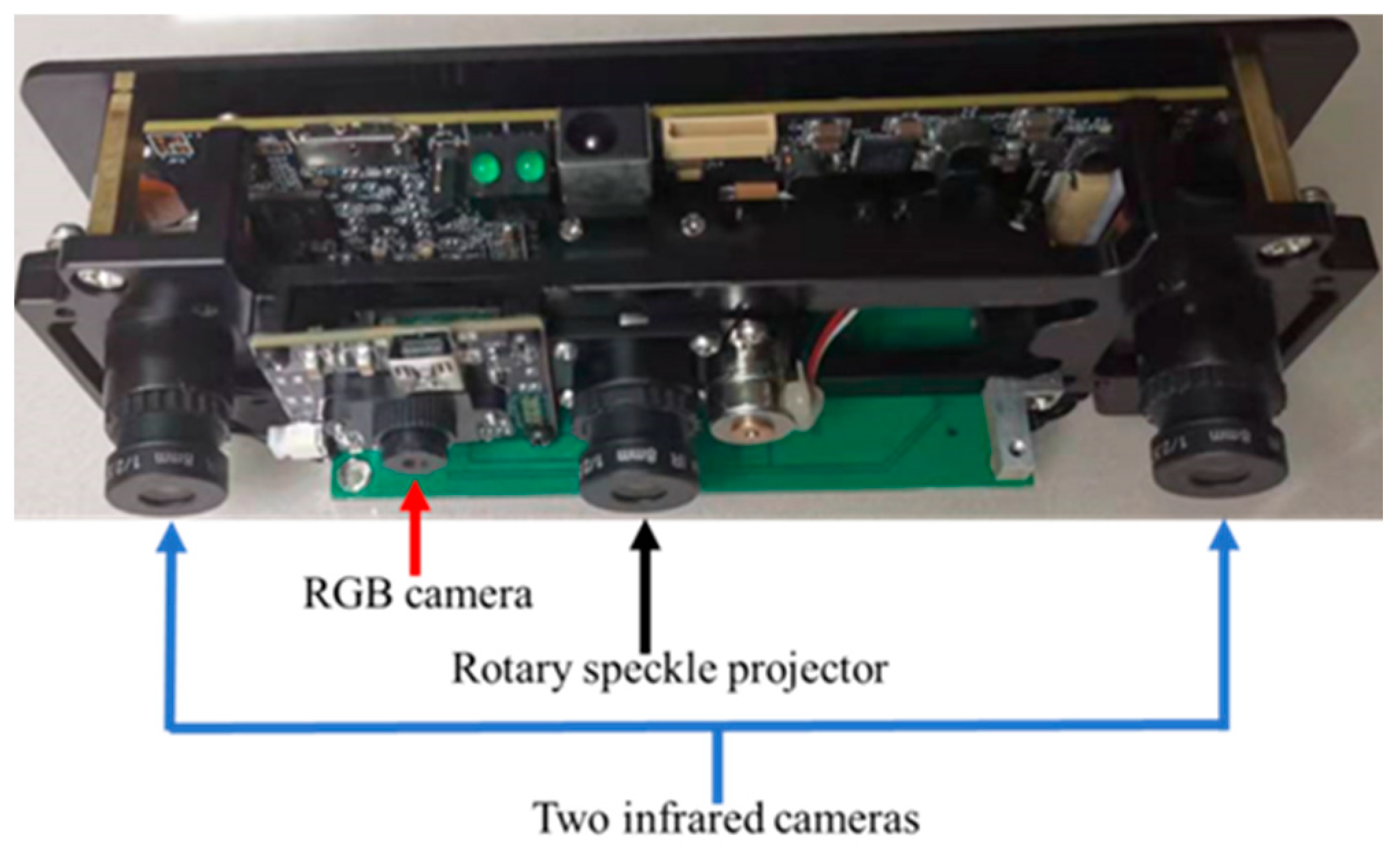
6.1. Setup

All experiments are carried out on a PC configured with Intel Core i7-8750H CPU (2.2 GHz) and 16G RAM. The STMCF and parameter optimization method are implemented using C++ by Visual Studio 2015. The value of each parameter in STMCF is set according to the result obtained by the parameter optimization method, as listed in Table 3. All parameters are kept constant in the following experiments.

Table 3. The specific value of each parameter in STMCF.

No.	Name	Optimized Value
1	R	1
2	Eps	0.8207
3	W_AD	0.3032
4	W_Census	0.2307
5	W_grad_x	0.9224
6	W_grad_y	0.6365
7	cen_win_h	5
8	cen_win_w	13
9	T_ad	0.4330
10	T_census	0.4155
11	T_grad_x	0.0646
12	T_grad_y	0.1515

Speckle stereo image pairs are acquired by the device presented in Figure 4. Sequence of different speckle patterns are generated and projected to the measured object by the rotary speckle projector in which a pseudo-random speckle pattern mask is inside. When two infrared cameras (the baseline is 120 mm, the focal length is 8 mm, the resolution is 1280 × 1024) capture images synchronously, the mask will stop rotating. Afterwards, the mask continues to rotate at a certain angle (~${10}^{\circ }$) and generate another pattern. The switching time between different speckle patterns is 11 ms and the exposure time of the camera is 2 ms. Therefore, the acquisition time for each speckle image pair is 13 ms. The number of speckle patterns can be set in the range of 3–12. The two infrared cameras are calibrated by the method proposed in [32] and the obtained camera parameters are used to rectify the speckle stereo image pairs.

Figure 4. Device of speckle stereo image pairs acquisition.

6.2. Effectiveness of the Proposed Gradient Computing Method

To verify the effectiveness of the proposed gradient computing method, the experiment is conducted to make comparison on reconstruction accuracy between two gradient computing methods: one includes the gradient of the guided image, the other does not. It is notable that the two methods use their own optimized values of parameters. A dumbbell gauge referred to the Germany guide line VDI VDE2634 Part2 [33] and is used for accuracy evaluation, as shown in Figure 5.

Figure 5. A dumbbell gauge.

The sphere diameter d_A = 50.7784 mm, d_B = 50.7856 mm and sphere center distance D = 100.0480 mm. The distance between the dumbbell gauge and projector is ~550 mm, the disparity range is −100 to 100, which is the same as other measured objects.

Table 4 shows a comparison of the results by projecting N speckle patterns (the bold figure indicates result with lower error, the same below). Note that points with large error near the boundary are deleted and the measured results are obtained by employing the commercial software Geomagic Studio. It can be seen from Table 4 that after including the gradient of the guided image, the errors are all decreased to varying degrees. Specifically, the error of sphere diameters d_A, d_B and sphere center distance D are reduced by 39.4%, 74.5% and 18.6% on average, respectively. Above data prove that the proposed gradient computing method is effective.

Table 4. Accuracy comparison between two gradient computing methods by measuring a dumbbell gauge. (Unit: mm).

N	Method	Abs.Err (1) (dA)	Abs.Err (dB)	Abs.Err (D)
3	Not (2)	0.0733	0.0794	0.0496
	Include (3)	0.0282	0.0140	0.0315
6	Not	0.0370	0.0871	0.0480
	Include	0.0255	0.0101	0.0445
9	Not	0.0256	0.0860	0.0629
	Include	0.0113	0.0471	0.0487
12	Not	0.0429	0.0681	0.0475
	Include	0.0390	0.0123	0.0436

⁽¹⁾ Abs.Err = Absolute value of error. ⁽²⁾ Not include the gradient of the guided image.⁽³⁾ Include the gradient of the guided image.

6.3. Experimental Comparison with the State-of-the-Art Method Based on Spatiotemporal Correlation

As one of the state-of-the-art methods based on spatiotemporal correlation, the spatiotemporal zero-mean normalized cross correlation (STZNCC) is widely used in random speckle 3D reconstruction [16,25,34,35]. To validate the performance of STMCF, a series of comparative experiments between STZNCC and STMCF are carried out.

6.3.1. Comparison of Reconstruction Accuracy

Firstly, the dumbbell gauge mentioned in Section 6.2 is used for accuracy comparison. The errors of measured results by projecting N speckle patterns are listed in Table 5.

Table 5. Accuracy comparison between STZNCC and STMCF by measuring a dumbbell gauge (Unit: mm).

N	Method	Abs.Err (dA)	Abs.Err (dB)	Abs.Err (D)
3	STZNCC	0.0518	0.0120	0.0316
	STMCF	0.0282	0.0140	0.0315
6	STZNCC	0.0613	0.0414	0.0533
	STMCF	0.0255	0.0101	0.0445
9	STZNCC	0.0305	0.0743	0.0580
	STMCF	0.0113	0.0471	0.0487
12	STZNCC	0.0519	0.0551	0.0530
	STMCF	0.0390	0.0123	0.0436

The results indicate that although when N = 3, the error of STMCF is a little greater than that of STZNCC in terms of d_B, the rest of the errors of STMCF are lower than STZNCC. Especially for N = 6, 9 and 12, the advantage is more obvious; the error of d_A, d_B and D, are at least 24.9% (N = 12), 36.6% (N = 9) and 16.0% (N = 9) lower than STZNCC, respectively.

To further evaluate reconstruction accuracy of the object with complex surface, a plastic human face mask (see Figure 6a) is also tested. Its ground truth (see Figure 6b) is obtained by the industrial scanner ATOS Core 300 (the measurement accuracy is ±0.02 mm, certified by the Germany guide line VDI VDE2634 Part2 [33]). The Geomagic Studio is employed to compare the differences between the reconstruction result and ground truth quantitatively. The error statistics of results, respectively using STZNCC and STMCF by projecting N speckle patterns, are presented in Figure 7.

Figure 6. (a) A plastic human face mask; (b) Its ground truth obtained by ATOS Core 300.

Figure 7. Error statistics comparison between STZNCC and STMCF of measuring a plastic human face mask. (a) maximum error; (b) average error; (c) standard deviation.

It can be easily discovered from Figure 7 that with the increase of N, the errors of both STMCF and STZNCC tend to decrease. In Figure 7a, except for N = 12, the maximum errors of STMCF are all less than STZNCC. In Figure 7b,c, the performance of STMCF is better than STZNCC in all cases. Therefore, in general, the accuracy of reconstructing the human face mask using STMCF is higher than that of STZNCC.

Figure 8, Figure 9, Figure 10 and Figure 11 shows reconstruction results and corresponding error distribution maps of the plastic human face mask, respectively, using STMCF and STZNCC by projecting N (N = 3, 6, 9, 12) speckle patterns.

Figure 8. (a) 3D reconstruction result of the plastic human face (N = 3); (b) Corresponding error distribution map.

Figure 9. (a) 3D reconstruction result of the plastic human face (N = 6); (b) Corresponding error distribution map.

Figure 10. (a) 3D reconstruction result of the plastic human face (N = 9); (b) Corresponding error distribution map.

Figure 11. (a) 3D reconstruction result of the plastic human face (N = 12); (b) Corresponding error distribution map.

It can be observed from Figure 8, Figure 9, Figure 10 and Figure 11 that the quality of both results obtained by STMCF and STZNCC becomes better with the increase of N. Besides, by carefully comparing the error distribution maps between STZNCC and STMCF in Figure 8, Figure 9, Figure 10 and Figure 11, we can find that the result of STMCF is more accurate in most areas. Above conclusions are consistent with the results shown in Figure 7.

6.3.2. Comparison of Computation Time

The computation time comparison between STZNCC and STMCF by projecting N speckle patterns are illustrated in Figure 12. It is worth mentioning that both methods use the coarse-to-fine matching strategy proposed in [25].

Figure 12. Computation time comparison between STZNCC and STMCF by projecting N speckle patterns: (a) a dumbbell gauge; (b) a plastic human face mask.

The results show that the computation time of both STZNCC and STMCF will rise when N increases. Moreover, although when N = 12, the computation time for a dumbbell gauge of STMCF is slightly higher than that of STZNCC, the computation time of STMCF is less than STZNCC in most cases.

6.3.3. Comparison of Real Human Face Reconstruction

In order to further verify the performance of STMCF in actual application situations, the author’s face under various expressions is reconstructed by STMCF and compared with the results of STZNCC, as shown in Figure 13.

Figure 13. Comparison of real human face reconstruction respectively using (a) STMCF (N = 12); (b) STZNCC (N = 12).

By careful observation, it can be found that the results of STMCF display contour details of the human face as clearly as that of STZNCC. More importantly, the smoothness of major areas on the human face (such as forehead, cheek and chin) is significantly better than STZNCC. Therefore, the effect of 3D face reconstruction using STMCF is more realistic.

6.4. Discussion

This paper reports a novel random speckle 3D reconstruction scheme, in which STMCF is proposed and a parameter optimization method based on DE algorithm is designed. A series of experimental results show that compared with STZNCC, STMCF has advantages in accuracy, computation time and reconstruction quality. However, there are still several aspects which need to be discussed.

(1)

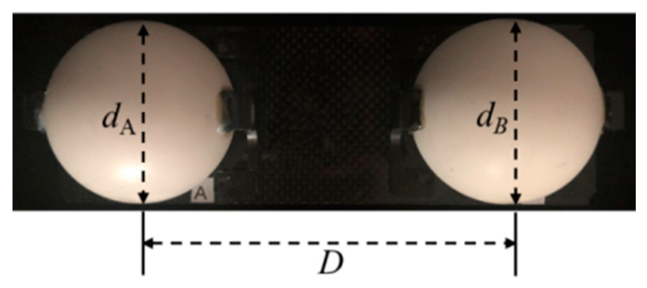
The error of d_A, d_B and D shown in Table 4 and Table 5 do not decrease with the increase of N, which is not consistent with the results presented in Figure 7. That is because the measured result of d_A, d_B and D are obtained by least square sphere fitting algorithm; similar results have also been reported in the literature [24]. Nevertheless, the error statistics shown in Figure 7 are calculated by a comparison between the reconstruction result and ground truth.

(2)

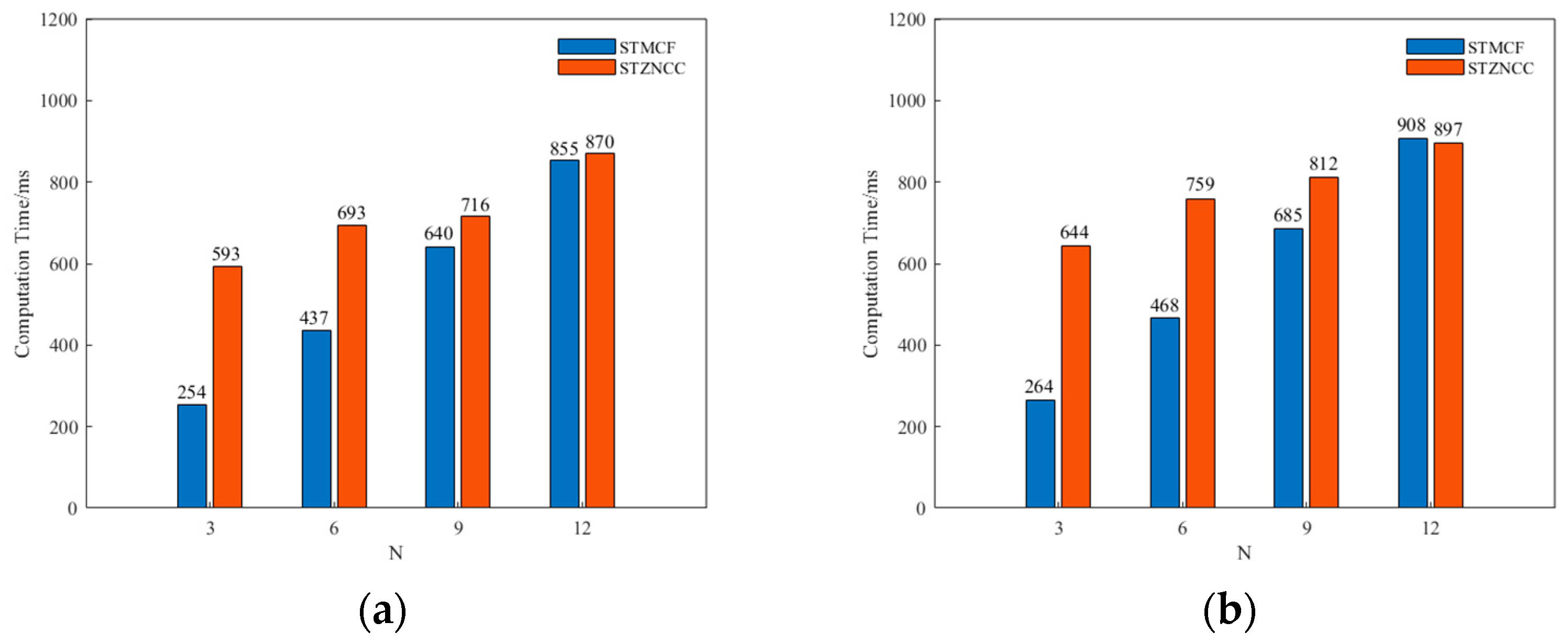
According to the results of Figure 12, on the whole, the performance of STMCF is better than STZNCC in terms of computation time. However, it is easily observable that the growth rate of STMCF in computation time is higher than that of STZNCC. So, when the value of N is smaller, the advantage of STMCF in computation time is more obvious.

(3)

Since there is no suitable training data with ground truth, a training strategy is explored in this paper. Experimental results validate the effectiveness of the strategy. This shows that the training results acquired from passive stereo vision data can be applied to the stereo matching of speckle stereo image pairs when the image acquisition environment is similar. The above conclusion can be helpful for other relative research works.

7. Conclusions

A novel random speckle 3D reconstruction scheme is presented. In this scheme, STMCF is proposed for stereo matching of speckle stereo image pairs. Besides, to automatically determine the values of all parameters included in STMCF, a parameter optimization method based on DE algorithm is designed and a training strategy is explored in this method. Experimental results demonstrate that our scheme can achieve accurate and high-quality 3D reconstruction efficiently and the performance of STMCF outperforms the state-of-the-art method based on spatiotemporal correlation, which is widely used in random speckle 3D reconstruction. At present, STMCF cannot meet the requirements for real-time application. In future work, we intend to reduce the computation time by hardware acceleration and apply it to 3D reconstruction of the dynamic indoor scene.

References

- Molleda, J.; Usamentiaga, R.; García, D.F.; Bulnes, F.G.; Espina, A.; Dieye, B.; Smith, L.N. An improved 3D imaging system for dimensional quality inspection of rolled products in the metal industry. Comput. Ind. 2013, 64, 1186–1200. [Google Scholar] [CrossRef]
- Du, G.; Zhou, M.; Ren, P.; Shui, W.; Zhou, P.; Wu, Z. A 3D modeling and measurement system for cultural heritage preservation. In Proceedings of the International Conference on Optical and Photonic Engineering, Singapore, 14–16 April 2015; p. 952420. [Google Scholar]
- Gherardini, F.; Leali, F. A framework for 3D pattern analysis and reconstruction of Persian architectural elements. Nexus Netw. J. 2016, 18, 133–167. [Google Scholar] [CrossRef] [Green Version]
- Microsoft, Kinect for Windows. Available online: https://developer.microsoft.com/en-us/windows/kinect (accessed on 14 April 2022).
- Kolmogorov, V.; Zabih, R. Computing visual correspondence with occlusions using graph cuts. In Proceedings of the Eighth IEEE International Conference on Computer Vision, Vancouver, BC, Canada, 7–14 July 2001; pp. 508–515. [Google Scholar]
- Sun, J.; Zheng, N.N.; Shum, H.Y. Stereo matching using belief propagation. IEEE Trans. Pattern Anal. Mach. Intell. 2003, 25, 787–800. [Google Scholar]
- Hirschmuller, H. Stereo processing by semiglobal matching and mutual information. IEEE Trans. Pattern Anal. Mach. Intell. 2008, 30, 328–341. [Google Scholar] [CrossRef]
- Scharstein, D.; Szeliski, R.; Zabih, R. A taxonomy and evaluation of dense two-frame stereo correspondence algorithms. In Proceedings of the IEEE Workshop on Stereo and Multi-Baseline Vision, Kauai, HI, USA, 9–10 December 2001; pp. 131–140. [Google Scholar]
- Kim, S.; Min, D.; Kim, S.; Sohn, K. Unified confidence estimation networks for robust stereo matching. IEEE Trans. Image Processing 2019, 28, 1299–1313. [Google Scholar] [CrossRef]
- Chang, J.R.; Chen, Y.S. Pyramid stereo matching network. In Proceedings of the IEEE Conference on Computer Vision and Pattern Recognition, Salt Lake City, UT, USA, 18–23 June 2018; pp. 5410–5418. [Google Scholar]
- Bouquet, G.; Thorstensen, J.; Bakke, K.A.H.; Risholm, P. Design tool for TOF and SL based 3D cameras. Opt. Express 2017, 25, 27758–27769. [Google Scholar] [CrossRef] [Green Version]
- Zhang, S. High-speed 3D shape measurement with structured light methods: A review. Opt. Lasers Eng. 2018, 106, 119–131. [Google Scholar] [CrossRef]
- Zuo, C.; Feng, S.; Huang, L.; Tao, T.; Yin, W.; Chen, Q. Phase shifting algorithms for fringe projection profilometry: A review. Opt. Lasers Eng. 2018, 109, 23–59. [Google Scholar] [CrossRef]
- Zhou, P.; Zhu, J.P.; Jing, H.L. Optical 3-D surface reconstruction with color binary speckle pattern encoding. Opt. Express 2018, 26, 3452–3465. [Google Scholar] [CrossRef]
- Keselman, L.; Woodfill, J.I.; Grunnet-Jepsen, A.; Bhowmik, A. Intel®RealSense™ Stereoscopic Depth Cameras. In Proceedings of the IEEE Conference on Computer Vision and Pattern Recognition Workshops, Honolulu, HI, USA, 21–26 July 2017; pp. 1267–1276. [Google Scholar]
- Zhou, P.; Zhu, J.P.; Xiong, W.; Zhang, J.W. 3D face imaging with the spatial-temporal correlation method using a rotary speckle projector. Appl. Opt. 2021, 60, 5925–5935. [Google Scholar] [CrossRef]
- Mei, X.; Sun, X.; Zhou, M.; Jiao, S.; Wang, H.; Zhang, X.P. On building an accurate stereo matching system on graphics hardware. In Proceedings of the IEEE International Conference on Computer Vision Workshops, Barcelona, Spain, 6–13 November 2011; pp. 467–474. [Google Scholar]
- Zabih, R.; Woodfill, J. Non-parametric local transforms for computing visual correspondence. In Proceedings of the European Conference on Computer Vision, Stockholm, Sweden, 2–6 May 1994; pp. 151–158. [Google Scholar]
- Hosni, A.; Rhemann, C.; Bleyer, M.; Rother, C.; Gelautz, M. Fast cost-volume filtering for visual correspondence and beyond. IEEE Trans. Pattern Anal. Mach. Intell. 2013, 35, 504–511. [Google Scholar] [CrossRef] [PubMed]
- Hamzah, R.A.; Ibrahim, H.; Abu Hassan, A.H. Stereo matching algorithm based on per pixel difference adjustment, iterative guided filter and graph segmentation. J. Vis. Commun. Image Represent. 2017, 42, 145–160. [Google Scholar] [CrossRef]
- Hong, P.N.; Ahn, C.W. Robust matching cost function based on evolutionary approach. Expert Syst. Appl. 2020, 161, 113712. [Google Scholar] [CrossRef]
- Gu, F.F.; Song, Z.; Zhao, Z. Single-shot structured light sensor for 3D dense and dynamic reconstruction. Sensors 2020, 20, 1094. [Google Scholar] [CrossRef] [Green Version]
- Yin, W.; Hu, Y.; Feng, S.; Huang, L.; Kemao, Q.; Chen, Q.; Zuo, C. Single-shot 3D shape measurement using an end-to-end stereo matching network for speckle projection profilometry. Opt. Express 2021, 29, 13388–13407. [Google Scholar] [CrossRef]
- Tang, Q.; Liu, C.; Cai, Z.; Zhao, H.; Liu, X.; Peng, X. An improved spatiotemporal correlation method for high-accuracy random speckle 3D reconstruction. Opt. Lasers Eng. 2018, 110, 54–62. [Google Scholar] [CrossRef]
- Fu, K.; Xie, Y.; Jing, H.L.; Zhu, J.P. Fast spatial-temporal stereo matching for 3D face reconstruction under speckle pattern projection. Image Vis. Comput. 2019, 85, 36–45. [Google Scholar] [CrossRef]
- Harendt, B.; Große, M.; Schaffer, M.; Kowarschik, R. 3D shape measurement of static and moving objects with adaptive spatiotemporal correlation. Appl. Opt. 2014, 53, 7507–7515. [Google Scholar] [CrossRef]
- Kong, L.Y.; Zhu, J.P.; Ying, S.C. Stereo matching based on guidance image and adaptive support region. Acta Opt. Sin. 2020, 40, 0915001. [Google Scholar] [CrossRef]
- He, K.M.; Sun, J.; Tang, X. Guided image filtering. IEEE Trans. Pattern Anal. Mach. Intell. 2013, 35, 1397–1409. [Google Scholar] [CrossRef]
- Haller, I.; Nedevschi, S. Design of Interpolation Functions for Subpixel-Accuracy Stereo-Vision Systems. IEEE Trans. Image Processing 2012, 21, 889–898. [Google Scholar] [CrossRef] [PubMed]
- Scharstein, D.; Hirschmüller, H.; Kitajima, Y.; Krathwohl, G.; Nešić, N.; Wang, X.; Westling, P. High-resolution stereo datasets with subpixel-accurate ground truth. In Proceedings of the German Conference on Pattern Recognition, Munich, Germany, 2–5 September 2014; pp. 31–42. [Google Scholar]
- Tanabe, R.; Fukunaga, A.S. Improving the search performance of shade using linear population size reduction. In Proceedings of the IEEE Congress on Evolutionary Computation, Beijing, China, 6–11 July 2014; pp. 1658–1665. [Google Scholar]
- Zhang, Z. A flexible new technique for camera calibration. IEEE Trans. Pattern Anal. Mach. Intell. 2000, 22, 1330–1334. [Google Scholar] [CrossRef] [Green Version]
- Optical 3-D Measuring Systems—Optical Systems Based on Area Scanning: VDI/VDE 2634 Blatt 2-2012; Beuth Verlag: Berlin, Germany, 2012.
- Zhou, P.; Zhu, J.P.; You, Z.S. 3-D face registration solution with speckle encoding based spatial-temporal logical correlation algorithm. Opt. Express 2019, 27, 21004–21019. [Google Scholar] [CrossRef] [PubMed]
- Xiong, W.; Yang, H.Y.; Zhou, P.; Fu, K.R.; Zhu, J.P. Spatiotemporal correlation-based accurate 3D face imaging using speckle projection and real-time improvement. Appl. Sci. 2021, 11, 8588. [Google Scholar] [CrossRef]