Quantifying Privacy Risks for Continuous Trait Data

Abstract

In the context of life sciences, the rapid biotechnical development leads to the creation of huge amounts of biological data. The use of such data naturally brings concerns on human genetic privacy breaches, which also discourage biological data sharing. Prior studies have investigated the possibility of the privacy issues associated with individuals’ trait data. However, there are few studies on quantitatively analyzing the probability of the privacy risk. In this paper, we fill this void by proposing a scheme for systematically breaching genomic privacy, which is centered on quantifying the probability of the privacy risk of continuous trait data. With well-designed synthetic datasets, our theoretical analysis and experiments lead to several important findings, such as: (i) The size of genetic signatures and the sensitivity (true positive rate) significantly affect the accuracy of re-identification attack. (ii) Both the size of genetic signatures and the minor allele frequency have a significant impact on distinguishing true positive and false positive matching between traits and genetic profiles. (iii) The size of the matching quantitative trait locus dataset has a large impact on the confidence of the privacy risk assessment. Validation with a real dataset shows that our findings can effectively estimate the privacy risks of the continuous trait dataset.

1. Introduction

Since the HapMap Project [1], genome sequencing has undergone considerable development with advancements that can greatly reduce the time and material expenses of DNA profiling that promote the development of bioinformatics [2,3,4]. Quantitative Trait Loci (QTL) [5], which is based on bioinformatics, is now a proven technique for large-scale biodata analysis [6] and is not only conducted in academic research but also widely commercialized as supporting services for direct-to-consumer DNA testing [7,8]. For example, QTL analysis revealed the presence of genetic mutations highly associated with cancer incidence [9,10,11].

While the resulting large amounts of data can facilitate revolutionary advancements in medical science and healthcare [12], the risk of genomic privacy breach has become an important concern, which arises when using and sharing genomic data because such data contains a series of information related to personal and familial privacy [13]. A unique threat posed by genomic data is that an individual’s genomic information not only breaches the privacy of the individual in question but also exposes a substantial amount of information about the individual’s relatives [14,15]. Combining with reidentification privacy risks by matching anonymized medical data with public genomic data [16,17], genomic privacy breaches will have long-term adverse effects on individuals and their families.

For the reasons above, both the executive branch and academia have paid increasing attention to genomic privacy. The US health care system has established strict privacy rules for the usage of genomic data [18], while the community website GenomePrivacy.org integrate genome privacy and security information for academic studies [19]. On the other hand, academic research has identified genomic privacy breaches or reidentification risks [20,21,22]. Specifically, Schadt et al. [20] used the top 1000 cis eQTLs for reidentification on an expression database from the entire US population and achieved a Type 1 error of ${10}^{-5}$ (wrongly identifying an innocent individual as a victim) and an accuracy of $85\%$. Backes et al. [21] achieved a reidentification accuracy of $97.5\%$ by relating DNA methylation data with genomic methylation Single Nucleotide Polymorphism (SNP) data. Sero et al. [22] designed face-to-DNA classifiers to associate face images and genomic data, demonstrating substantial true matching (training accuracy $83\%$, verification accuracy $80\%$).

However, previous studies only focus on qualitatively analyzing whether potential re-identification risks exist, but few studies have quantitatively analyzed under what circumstances re-identification risks exist. Eric E Schadt et al. [20], Lippert et al. [23], and Michael Backes et al. [21] focused on the possibility of privacy threat between DNA and phenotypes; all of their quantitative analyses were intended to illustrate the existence of the privacy threat, with little mention of how serious the privacy risks was in different situations. Furthermore, all the previous studies are limited to a certain class of continuous trait data. Lippert et al. [23] limited their quantitative models for just a few common phenotypes, Eric E Schadt et al. [20] only verified the privacy risks of RNA expression data, Michael Backes et al. [21] only estimated identification risks of methylation data with small overlap between distributions. In general, previous works had not proposed a method to predict the privacy risk of any set of continuous traits.

Contributions. In this paper, we provide the first detailed quantitative derivation for the probability of the privacy risks of continuous trait data, which can be used to measure the vulnerability, the probability that the data will be unable to resist the privacy-breaching attack [24]. Our contributions can be divided into three major areas. (i) We formalize the genome privacy breaching attack as a series of single-feature three-classification problems. This formalization also allows us to construct synthetic data with configurable parameters, which is needed because our quantitative analysis requires parameters that can be set. Moreover, there are few real-world data for testing our approaches. (ii) We present a Bayesian method that matches continuous trait profiles to the genotypes. This allows us to draw deeper insights, such as: the factor affecting the matching accuracy does not depend on the accuracy of classification but depends on the sensitivity (see Section 6.3.1) and the number of continuous traits; both the prior probabilities of genotypes and the number of continuous traits have significant impacts on distinguishing true positive and false positive matching; the larger the matching dataset, the lower the privacy risk. (iii) Our analysis of the real dataset confirms that with sensitivity, the number of traits, and the prior probabilities of genotypes, we can accurately estimate the privacy implications of a trait dataset.

Organization. We introduce the background knowledge about traits and genotypes in Section 2, review the relevant previous work in Section 3, present our adversarial model in Section 4, and then describe the principle of synthetic data generation in Section 5. In Section 6, we analyze the main factors affecting data privacy risk through simulation experiments and mathematical derivation and verified our analysis results with real data. We also discuss the application scenarios of our findings and what needs to be improved in future work in Section 7, before concluding in Section 8.

2. Preliminaries

In this section, we review three biological concepts that are used throughout the paper. The concept of SNP is used for describing the differences between individual genes. The concept of QTL describes the association between epigenetic characteristics and genes. The concept of MAF reflects the prior probability of different genes.

2.1. SNP (Single Nucleotide Polymorphism)

SNP is an important concept in the context of the present paper because it can be exploited for genomic privacy breaching. This is possible because SNP is the most common and representative heritable genetic variant. An SNP is the variation of a single nucleotide in DNA; this variation can be a transition (e.g., Cytosine to Thymine) or transversion (e.g., Cytosine to Adenine) of a single nucleotide. SNPs are effectively the digenic type in most cases [25]; each SNP usually contains two alleles, called major and minor alleles, respectively. Studies show that there are strong correlations between SNPs and some specific diseases, such as the incidence of Alzheimer’s disease, which is highly correlated with particular SNPs [26]. This means that for genomic privacy breaching or reidentification purposes, an attacker does not need to use the entire DNA sequence; rather, the attacker only needs to consider DNA variations, which can be effectively measured via SNPs.

2.2. QTL (Quantitative Trait Loci)

A QTL is a region of the genome that is associated with a particular phenotypic trait, which can be attributed to a polygenic effect [27]. At a high level, the QTLs that are located near their original genes are known as cis QTLs, whereas the ones that are located far from their original genes are known as trans QTLs. To reduce the impact that the sample sizes of many QTL studies are small [28], researchers have combined QTLs and global gene expression for mapping the genetic features to expressions from numerous transcripts [29].

2.3. MAF (Minor Allele Frequency)

The MAF is the prior probabilities of SNPs’ rare variants from a given population [30,31]. A digenic SNP can be considered as a combination of independent DNA bases A and B with occurrence probability $Pr\left(A\right)$ and $Pr\left(B\right)$ such that $Pr\left(A\right)+Pr\left(B\right)=1$. Then the MAF is the minor value of $Pr\left(A\right)$ and $Pr\left(B\right)$. Let $AA$ denote the case or event where SNP takes the value $(A,A)$, $BB$ denote the case where SNP takes the value $(B,B)$, and $AB$ denote the case where SNP takes the value $(A,B)$ or $(B,A)$. We have $Pr\left(AA\right)=Pr{\left(A\right)}^2$, $Pr\left(BB\right)=Pr{\left(B\right)}^2$, and $Pr\left(AB\right)=2Pr\left(A\right)Pr\left(B\right)$ as A and B are independent.

3. Related Work

In the context of the present paper, genomic privacy risk can be mainly divided into several scenarios, such as the $n=1$ scenario, the summary statistic scenario, and the gene expression scenario, etc.

Studies in the $n=1$ scenario. In this scenario, the sensitive traits are correlated with individual’s genotype directly [32]. Several attacks have been proposed for this scenario. Pakstis et al. [33] discovered that approximately 45 carefully chosen SNPs could be used for major global population identification with a type 1 error of ${10}^{-15}$. More generally, Zhen Lin et al. [34] summarized the influence of matching accuracy with the average MAF, number of SNPs and population, measured the TPR and FPR of predicitons correlated to these parameters in the $n=1$ scenario, and revealed that a random subset of approximately 300 SNPs with an MAF $⩽0.1$ was sufficient to uniquely identify any person around the world. A more recent study on Beacon [35] demonstrate that only 1000 “yes or no” queries for SNPs can detect the presence of an individual from the Personal Genome Project [36]. To against this situation, in a study on methylation data sharing in Beacon, Inken Hagestedt et al. [37] proposed the MBeacon system for private DNA methylation data sharing with a comparison test.

Studies in the summary statistic scenario. In this scenarios, Compared with the allele frequencies of the general population, allele frequencies from the case group will be positively biased toward the target genotypes [32], which was investigated in a landmark study by Nils Homer et al. [38], who found that ADAD on GWAS data could be achieved only with the study participants’ allele frequencies. Subsequent researches expanded the scope of the vulnerabilities for summary statistics and analysed its mathematical properties [39,40,41].

Studies in the gene expression scenario. In this scenarios, gene expressions that are linked to a series of attributes, such as QTL data, could be used for genomic privacy breaching. As Eric E Schadt et al. mentioned [20], with a training step using a standard reference eQTL data set, a Bayesian approach could be used to calculate the probability distributions of the expression data with given genotypes. The researchers then matched the target genotype and tested the TPR and FPR of this matching. with the top 1000 cis eQTLs, this ADAD technique had high accuracy in large-scale simulations. Robert A Philibert et al. [42] notably emphasized this scenario with specific methylation data. Stephanie O. M. Dyke et al. [43] described the biomolecular mechanism by which methylation data could lead to a privacy risk by analysing real data. Subsequently, Michael Backes et al. [21] used the Bayesian method adapted from As Eric E Schadt’s work [20] to correlate the methylation profile to an individual genotype, which had an up to $97.5\%$ matching accuracy with 293 independent meQTL-methylation pairs and without false positive predictions on a dataset of nearly 3000 samples. They also proved that the continuous distribution function could be best fixed as a normal distribution, which supports the findings of our simulation experiments. Lippert et al. [23] used 1062 volunteer samples for analysis and found that the associations between some common phenotypes and genes could lead to privacy threats. The findings of a more resent study from Dzemila Sero et al. [22], who used high-resolution 3D facial data and correlated them with SNP profiles, was challenged by Rajagopal Venkatesaramani et al. [44] in terms of the actual feasibility.

Studies in the other scenarios. Regarding genomic privacy breaches, several papers have studied privacy risks related to various sorts of additional data or in spatial conditions with large-scale spatio-temporal extents. Gymrek et al. showed that genotypes can be reidentified with genetic traits on the Y chromosome by querying genetic genealogy databases [45]. Humbert et al. showed that SNPs can also be exploited to further reidentify anonymous genotypes by typically using side channels [14]. Backes et al. proposed a model for quantifying the impact of the continuous sequencing and publicizing of personal genomic data on a population’s genomic privacy [46], which demonstrated that an increasing sharing rate in the future will entail a substantial negative effect on the privacy of all older generations. Berrang et al. presented a generic framework for quantifying the privacy risks in biomedical data taking into account the various interdependencies between data of different types, from different individuals, and at different times [47]. With this framework, an adversary can efficiently identify the parent-child relationships based on methylation data with a success rate of $95\%$.

4. Model and Methodology

To characterize the privacy risks of anonymous continuous trait data without protection, we propose a privacy-breaching attack method that can reveal sensitive personal information based on a calculated approach while leveraging publicly available data. In this section, we first introduce adversarial models for privacy breaching and then introduce our attack methods.

4.1. Threat Model

We consider a scenario where the adversary has access to both genetic data and continuous trait data. The continuous trait data is anonymous, while some shareable genetic profiles have real identifiers, such as information that can be targeted to specific individuals. Examples of genetic databases include OpenSNP [16] and the Personal Genome Project [17]. This information can be taken by the adversary to re-identify personal information from other anonymous continuous trait data [48]. Furthermore, even if a genetic profile is anonymous, the adversary can still link it to its pedigree with surname-genome associations [45], kinships [14], or online social networks [49].

We assume a threat model under which the correlations between continuous traits and SNPs may be acquired as the background knowledge by the adversary, as shown in Figure 1. First, there are two ways for an adversary to obtain this background knowledge. One approach is to obtain the relationships by analyzing public QTL datasets, such as the cerebrospinal fluid proteome dataset in National Center for Biotechnology Information (NCBI) [48]. The other approach is to rely on existing findings of the statistical relationships between genes and continuous traits. For example, the adversary can obtain prior probabilities, expectations, and standard deviations of RNA-binding proteins (RBP) with disease-related SNPs from academic QTLs websites [50]. Next, the adversary needs to determine whether the individual genomic profile is the member of the continuous trait dataset, and if so, which individual. Finally, the adversary successfully matches continuous trait profile and genotype as the same individual, which leads to privacy breaches.

Figure 1. Privacy-breaching model for trait-gene profile reidentification. The adversary first infers the correlations between continuous trait data and gene data (central box) with training datasets (upper box left) or existing research results (upper box right) and then maps the anonymous continuous trait profile (coloured with black in the left box) to the genotype (coloured with orange in the right box) with correlation obtained for reidentification. Then, the adversary verifies whether an individual with the continuous trait data is the member of the genotype dataset. If the matching between the continuous trait profile and genotype is sufficiently significant, it is considered correct (lower box, reidentified individuals are indicated as human shapes with the same colour of that in the right box). Each human shape represent an individual; each trait data or gene data in a box represent a continuous trait profile or a genotype profile from an individual.

4.2. Attack Methodology

The continuous trait data and SNP data can be presented as a $m_t\times n_t$ array $\mathbb{T}$ and a $m_s\times n_s$ array $\mathbb{S}$, respectively. The k-th column in $\mathbb{T}$, denoted by $\mathbb{T}(·,k)$, contains individual k’s all continuous traits, and the i-th row in $\mathbb{T}$, denoted by $\mathbb{T}(i,·)$ contains i-th continuous trait for all individuals. Similarly, $\mathbb{S}(·,l)$ and $\mathbb{S}(j,·)$ represent the individual l’s genomic profile and j-th SNP for all individuals respectively. In general, the number of the genetic loci is much larger than the number of continuous traits (i.e., $j\gg i$). It has been shown that there are multiple $\mathbb{S}(j,·)$ corresponding to one $\mathbb{T}(i,·)$ as QTLs in the vast majority of cases [48]. Let $\Omega \left(i\right)$ be an index set for the SNPs that are correlated with the i-th continuous trait. Then $\mathbb{S}(\Omega (i),l)$ contains the values of SNPs that are correlated with the i-th continuous trait for individual l.

The deanonymization attack contains two stages. In the first stage, the adversary obtains the prior probabilities, expectations, and standard deviations as the correlations between $\mathbb{S}(\Omega (i),·)$ and $\mathbb{T}(i,·)$. In the next stage, based on this knowledge, the adversary is able to identify the best-matched pair $\{\mathbb{S}(·,l^{\ast }),\mathbb{T}(·,k^{\ast })\}$ and determine whether the SNP profile $\mathbb{S}(·,l^{\ast })$ and continuous trait profile $\mathbb{T}(·,k^{\ast })$ belong to the same person.

As mentioned in Section 4.1, There are two approaches for the adversary to acquire correlations between SNPs and continuous traits. For the second approach, the adversary can obtain the prior probabilities, expectations, and standard deviations directly; for the first approach, the probabilistic relationships between the continuous traits and genetic loci are derived through training data which are either publicly available or the adversary has access to, and is the focal point of this subsection. Note that the members of the continuous trait data correspond one-to-one with the members of the SNP data in the training set, for example, $\mathbb{T}(·,k)$ and $\mathbb{S}(·,k)$ are from the same individual. In addition, for the training set, each SNP in corresponding to $\mathbb{S}(j,·)$ is corresponding to at least one continuous trait in $\mathbb{T}(i,·)$, while each continuous trait in $\mathbb{T}(i,·)$ has at least one corresponding SNP in $\mathbb{S}(j,·)$.

It should be noted that our approach is related to the works of Michael Backes et al. [21] and Eric E Schadt et al. [20]. However, these two studies limited their traits to certain types (methylation level and cis RNA level), while our approach adopts continuous traits that are more general. Furthermore, different from these two studies which approximately used normal distribution to estimate the probabilities of the continuous trait values at different genotypes, since most of the continuous trait values are greater than zero, we adopt a truncated normal distribution for $Pr\left(\mathbb{S}(j,l)\left|\mathbb{T}\right(i,k)\right)$ estimation that is more realistic. We will describe this approach in greater detail.

Let $T_i$ be a continuous random variable that measures the value of the i-th quantitative measure and let $S_{\Omega \left(i\right)}$ be the region of SNPs that are mostly correlated to $T_i$. The goal is to obtain the posterior probability for $S_{\Omega \left(i\right)}$ to take value $\mathbb{S}(\Omega (i),k)$ for an individual person k if $T_i$ takes value $\mathbb{T}(i,k)$ for the same person, that is, to obtain $Pr\left(S_{\Omega \left(i\right)}=\mathbb{S}(\Omega \left(i\right),k)|T_i=\mathbb{T}(i,k)\right)$ for any k. By the Bayes rule, we have

$$\begin{array}{c}\hfill \begin{array}{cc}\hfill & Pr\left(S_{\Omega \left(i\right)}=\mathbb{S}(\Omega \left(i\right),k)|T_i=\mathbb{T}(i,k)\right)\hfill \\ \hfill & =\frac{Pr\left(T_i=\mathbb{T}(i,k)|S_{\Omega \left(i\right)}=\mathbb{S}(\Omega \left(i\right),k)\right)Pr\left(S_{\Omega \left(i\right)}=\mathbb{S}(\Omega \left(i\right),k)\right)}{{\sum }_{i=1}^{m}Pr\left(T_i=\mathbb{T}(i,k)|S_{\Omega \left(i\right)}=\mathbb{S}(\Omega \left(i\right),k)\right)Pr\left(S_{\Omega \left(i\right)}=\mathbb{S}(\Omega \left(i\right),k)\right)}\hfill \end{array}\end{array}$$

(1)

To make $\mathbb{S}(\Omega (i),·)$ easier to handle, let $\mathbb{S}(\Omega (i),·)\approx \mathbb{S}(i,·)$, where the SNP represented by $\mathbb{S}(i,·)$ is the SNP that most relevant to $\mathbb{T}(i,·)$. Note that $i_1\ne i_2\iff \mathbb{T}(i_1,·)$$\ne \mathbb{T}(i_2,·),\mathbb{S}(i_1,·)\ne \mathbb{S}(i_2,·)$, then we have $m_s=m_t$ and $n_s=n_t$ for the training set. In Equation (1), $Pr\left(S_{\Omega \left(i\right)}=\mathbb{S}(\Omega \left(i\right),k)\right)$ can be calculated using MAF, which is mentioned in Section 2.3, and may also be available from genetic database such as dbSNP [51]. $Pr\left(T_i=\mathbb{T}(i,k)|S_{\Omega \left(i\right)}=\mathbb{S}(\Omega \left(i\right),k)\right)$ is characterized by a continuous conditional probability density $f_{T_i|S_{\Omega \left(i\right)}}$.

Both Michael Backes et al. [21] and Eric E Schadt et al. [20] verified that most of the continuous traits related to SNPs satisfied the normal distribution. However, unlike their solutions that used the normal distribution directly, since most continuous traits have non-negative values, the distribution with range $(0,+\infty )$ is more appropriate to model the continuous distribution functions. Specifically, let the mean and variance parameters of this truncated normal distribution be ${\mu }_i$ and ${\sigma }_i$, then its density is

$$\begin{array}{c}\hfill f_{T_i|{\mathbb{S}}_{\Omega \left(i\right)}}=\frac{1}{{\sigma }_i}\frac{\varphi \left(\frac{T_i-{\mu }_i}{{\sigma }_i}\right)}{1-\Phi \left(\frac{-{\mu }_i}{{\sigma }_i}\right)}=\frac{\varphi \left(\frac{T_i-{\mu }_i}{{\sigma }_i}\right)}{{\sigma }_i\Phi \left(\frac{{\mu }_i}{{\sigma }_i}\right)}\end{array}$$

where $\varphi (·)$ and $\Phi (·)$ are the probability density function (p.d.f.) and cumulative distribution function (c.d.f.) respectively.

4.3. Matching Attack

After acquiring correlations $Pr\left(T_i|S_{\Omega \left(i\right)}\right)$ for all pairs $\mathbb{T}(i,·)$ and $\mathbb{S}(i,·)$, we need to infer the individual links of the testing set between $m_t^{\prime }\times n_t^{\prime }$ continuous trait array ${\mathbb{T}}^{\prime }$ containing $n_t^{\prime }⩾1$ members and $m_s^{\prime }\times n_s^{\prime }$ SNP array ${\mathbb{S}}^{\prime }$ containing $n_s^{\prime }⩾1$ members. The members of ${\mathbb{Q}}^{\prime }$ and ${\mathbb{S}}^{\prime }$ may be different, where $n_t^{\prime }$ and $n_s^{\prime }$ are not necessarily equal; similarly with the training set, $\mathbb{T}(i,·)$ and ${\mathbb{T}}^{\prime }(i,·)$ are corresponding to the same continuous trait, and $\mathbb{S}(i,·)$ and ${\mathbb{S}}^{\prime }(i,·)$ are corresponding to the same SNP, then we have $m_s=m_t=m_s^{\prime }=m_t^{\prime }=m$.

The adversary needs to traverse the $n_t^{\prime }$ continuous trait samples and $n_s^{\prime }$ SNP samples to get the best match pairs $\{{\mathbb{S}}^{\prime }(·,l^{\ast }),{\mathbb{T}}^{\prime }(·,k^{\ast })\}$. For any pair of $\{{\mathbb{S}}^{\prime }(·,l^{\prime }),{\mathbb{T}}^{\prime }(·,k^{\prime })\}$, The adversary first calculates the trait propensity score $e{(l^{\prime },k^{\prime })}_i$ for each pair of $\{{\mathbb{S}}^{\prime }(i,l^{\prime }),{\mathbb{T}}^{\prime }(i,k^{\prime })\}$ through correlations $Pr\left(T_i|S_{\Omega \left(i\right)}\right)$, where $e{(l^{\prime },k^{\prime })}_i$ is defined as

$$\begin{array}{c}\hfill e{(l^{\prime },k^{\prime })}_i=Pr\left(S_{\Omega \left(i\right)}={\mathbb{S}}^{\prime }(i,l^{\prime })|T_i={\mathbb{T}}^{\prime }(i,k^{\prime })\right)\end{array}$$

(2)

Next, the adversary calculates the individual propensity score $e(l^{\prime },k^{\prime })$ as

$$\begin{array}{c}\hfill e(l^{\prime },k^{\prime })=\frac{1}{m}\sum _{i=1}^{m}e{(l^{\prime },k^{\prime })}_i\end{array}$$

(3)

Finally, after traversing all the scores of SNP samples $l^{\prime }$ and continuous trait samples $k^{\ast }$ paired, the adversary can know that the sample $l^{\ast }$ that best matches sample $k^{\ast }$ is

$$\begin{array}{c}\hfill l^{\ast }=arg\underset{l^{\prime }}{max}e(l^{\prime },k^{\ast })\end{array}$$

(4)

4.4. Best Matching Validation

To evaluate the significance of the individual propensity score, we define F Score $F_{k^{\prime }}$ for evaluation as

$$\begin{array}{c}\hfill F_{k^{\prime }}=\frac{e(l^{\prime },k^{\prime })-E\left[e(·,k^{\prime })\right]}{\mathrm{SD}\left[e(·,k^{\prime })\right]}\end{array}$$

(5)

where $e(·,k^{\prime })$ is the set of traversed individual propensity scores between ${\mathbb{T}}^{\prime }(·,k^{\prime })$ and ${\mathbb{S}}^{\prime }$; $E\left[e(·,k^{\prime })\right]$ is the expectation of $e(·,k^{\prime })$, and $\mathrm{SD}\left[e(·,k^{\prime })\right]$ is the standard deviation of the set. In fact, the F score $F_{k^{\prime }}$ is a standardized measurement for $e(l^{\prime },k^{\prime })$, which allows us to determine whether a continuous trait profile and its best-matched genotype are both from the same individual. Specifically, if ${\mathbb{T}}^{\prime }\cap {\mathbb{S}}^{\prime }=⌀$, the best matching score between the continuous trait profile and the SNP profile does not mean that these two profiles correspond to the same individual; in this case, we can detect these false positive matches with the F score. Moreover, even if $n_t^{\prime }$-by-$n_s^{\prime }$ matching becomes computationally infeasible, it is possible to remove false positive matches with F score.

5. Synthetic Data Generation

There are few real-world datasets we can use to test the feasibility of the attack systematically because of two reasons. The first one is parameter control. The prior probabilities of the genes, the expectation and standard deviation of the continuous traits corresponding to the genes, etc., are uncontrollable in a real QTL dataset, which are not conducive to quantitative analysis of privacy risks. The second one is access control. Due to the current strict access control restrictions, it is difficult to obtain real QTL data for non-biological or non-medical research [52]. Therefore, synthetic data generation is necessary to quantify the privacy risks of continuous traits. The next two subsections will describe the design and implementation of the synthetic data generator respectively.

5.1. Design of the Synthetic Data Generator

We formulate the following rules for our synthetic data generators:

(a)

Both continuous trait data and SNP data are sampled from the same population.

(b)

Each trait in continuous trait data has one and only one corresponding SNP in SNP data, and different traits do not correspond to the same SNP, and vice versa.

(c)

The continuous traits are related to SNP-based genes in three forms $AA$, $AB$, and $BB$, and the values of continuous traits corresponding to these three genotypes are all truncated normal distributions.

With these regulations, we will mention the implementation of our synthetic data generator in the next subsection.

5.2. Implementation of the Synthetic Data Generator

What our synthetic data generator needs to generate is the QTL dataset, which needs to generate the continuous trait data ${\mathbb{T}}^{\ast }$ and its corresponding SNP data ${\mathbb{S}}^{\ast }$. As described in our previous work [53], there are four steps for data generation:

First, we need to determine the structure of the dataset. Let $m_t^{\ast }=m_s^{\ast }=m$, $n_t^{\ast }=n_s^{\ast }$$=n$, and for $0<i⩽m,0<j⩽n$, let ${\mathbb{T}}^{\ast }(·,j)$ and ${\mathbb{S}}^{\ast }(·,j)$ be the same individual and let $\Omega \left(i\right)={\mathbb{S}}^{\ast }(i,·)$, which means that the most correlated SNP of ${\mathbb{T}}^{\ast }(i,·)$ is ${\mathbb{S}}^{\ast }(i,·)$. Then we pre-set the parameters $m,n$ for the synthetic data generator.

Next, we need to formalize the distributions of ${\mathbb{T}}^{\ast }(i,·)$ corresponding with ${\mathbb{S}}^{\ast }(i,·)$. We define $s_1,s_2,s_3\in \{AA,AB,BB\}\wedge s_1\ne s_2\ne s_3$. For each pair of ${\mathbb{T}}^{\ast }(i,·)$ and ${\mathbb{S}}^{\ast }(i,·)$, there are three distributions $f_{T_i^{\ast }|s_1},f_{T_i^{\ast }|s_2},f_{T_i^{\ast }|s_3}$. The expectations of three distributions are randomly generated as ${\mu }_{T_i^{\ast }|s_1},{\mu }_{T_i^{\ast }|s_2},{\mu }_{T_i^{\ast }|s_3}$, such that ${\mu }_{T_i^{\ast }|s_1}<{\mu }_{T_i^{\ast }|s_2}<{\mu }_{T_i^{\ast }|s_3}$.

We thirdly define the distance between two distributions. The distance between the two expectations ${\mu }_1$ and ${\mu }_2$ does not reflect the distance between distributions $f_1$ and $f_2$; even if the absolute value $|{\mu }_2-{\mu }_1|$ is very large, the larger standard deviations ${\sigma }_1$ and ${\sigma }_2$ will also make $f_1$ not far away from $f_2$. To accurately describe the distance between two distributions, we define the z-score z as the ratio between the difference of expectations ${\mu }_2-{\mu }_1$ and the sum of standard deviations ${\sigma }_1+{\sigma }_2$:

$$\begin{array}{c}\hfill z=\frac{{\mu }_2-{\mu }_1}{{\sigma }_1+{\sigma }_2}\end{array}$$

(6)

We also define $z_{\alpha }$ as the z-score of $f_{T_i^{\ast }|s_1}$ and $f_{T_i^{\ast }|s_2}$, $z_{\beta }$ as the z score of $f_{T_i^{\ast }|s_2}$ and $f_{T_i^{\ast }|s_3}$. For each synthetic QTL dataset, all pairs of ${\mathbb{T}}^{\ast }(i,·)$ and ${\mathbb{S}}^{\ast }(i,·)$ in one QTL dataset use the same setting of $z_{\alpha },z_{\beta }$. Then we pre-set the parameters $z_{\alpha },z_{\beta }$ for the synthetic data generator.

The final step is the generation of ${\mathbb{T}}^{\ast }(i,j)$ and ${\mathbb{S}}^{\ast }(i,j)$. Similarly with step 3, for each synthetic QTL dataset, all the $S(i,·)$ use the same setting of MAF value $p_{\mathrm{m}}$ to obtain the prior probability. The synthetic data generator first randomly generates the value of ${\mathbb{S}}^{\ast }(i,j)$ as $s_1,s_2,s_3$ based on the prior probability $p_{s_1},p_{s_2},p_{s_3}$, and then generates ${\mathbb{T}}^{\ast }(i,j)$ through the corresponding probability distribution $f_{T_i^{\ast }|{\mathbb{S}}^{\ast }(i,j)}$. At last, we need to pre-set the parameters $p_{\mathrm{m}}$ for the synthetic data generator.

As can be seen from the steps above, we need five parameters $m,n,z_{\alpha },z_{\beta },p_{\mathrm{m}}$ as the input for the synthetic data generation in order to generate a synthetic QTL dataset. Referring to the findings from previous studies [21,34,35,54], we choose four values for m as 50, 100, 200, and 300, respectively, and four values for n as 50, 100, 200, and 500, respectively. Similarly, referring to the relationship between standard deviation and cumulative probability in the standard normal distribution, we choose six values for both $z_{\alpha }$ and $z_{\beta }$ as $0.13$, $0.68$, $1.29$, $1.65$, $2.33$, and $2.58$, respectively, which are corresponding to cumulative probabilities as $55\%$, $75\%$, $90\%$, $95\%$, $99\%$, and $99.5\%$, respectively. For MAF values $p_{\mathrm{m}}$, we choose $0.05$, $0.15$, $0.30$, and $0.45$, to roughly cover the value range of MAF ($0<p_{\mathrm{m}}⩽0.5$). After executing data generation, we obtain a 2304-item continuous trait dataset ${\mathbb{T}}^{\ast }$ and its corresponding SNP dataset ${\mathbb{S}}^{\ast }$ with the same item count. We repeat the data generation process 10 times, obtaining 10 ${\mathbb{T}}^{\ast }$ continuous trait datasets and 10 correlated ${\mathbb{S}}^{\ast }$ SNP datasets.

6. Attack Validation

We present our detailed experimental steps and main results here using the dataset described in Section 5. In this section, we first describe and quantify the degree of influences from different parameters, then identify the most important factors for continuous trait data re-identification based on mathematical derivation analysis, and finally use a real QTL dataset to evaluate the feasibility of our estimation.

6.1. Training and Testing Sets

Consulting the limitations of real QTL studies that the sample sizes of QTL datasets are always small (around 100) [21,50,54], we design two training/testing experimental setups as follows: (a) select half of the QTL profiles randomly as the training set if the sample size $n⩽100$, and (b) select 50 QTL profiles randomly as the training set if the sample size $n>100$.

After random splitting and training, we estimate the posterior probability by mapping $n/2$ ($n⩽100$) or $n-50$ ($n>100$) continuous trait profiles for matching at a time with the n genotypes to evaluate the effectiveness of the re-identification attack. We repeat this splitting-training-matching process 5 times for each simulated QTL dataset (10 in total, mentioned in Section 5.2), resulting in 50 training/testing experiments for each parameter setting.

6.2. Matching Results

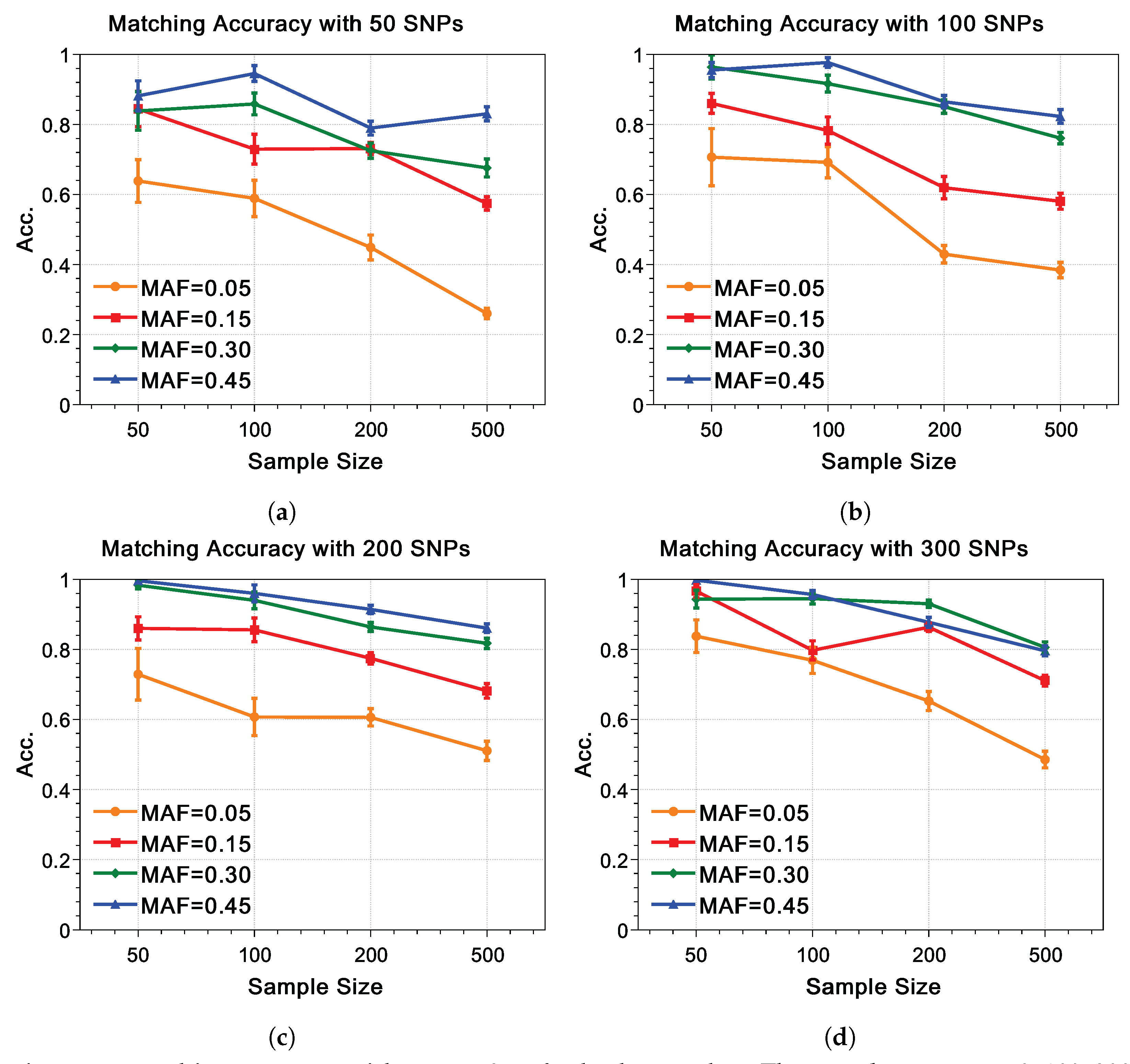
Since there are a large number of parameter settings, only typical results will be shown as figures. The matching accuracy with $z=2.33$ are shown in Figure 2, which demonstrates several tendencies:

Figure 2. Matching accuracy withz score$2.33$ for both $z_{\alpha }$ and $z_{\beta }$. The sample sizes n as 50, 100, 200, and 500 are expressed on the abscissa, respectively, while the matching accuracy is expressed on the ordinate. Matching accuracy with different MAFs and their standard deviations are expressed as different colored symbols with error bars, while the orange ellipse, red rectangle, olive diamond and blue triangle represent the MAF value of $0.05$, $0.15$, $0.30$ and $0.45$, respectively. The SNP sizes m of (a–d) are 50, 100, 200, and 300, respectively. (a) 50 SNP. (b) 100 SNP. (c) 200 SNP. (d) 300 SNP.

First, for all the SNP size m, the matching accuracy decreases as the size of the testing set increasing. Second, the matching accuracy decreases as the MAF value $p_{\mathrm{m}}$ decreases. This tendency appears in each sub-figure from Figure 2. If $p_{\mathrm{m}}⩾0.30$, this tendency also holds in most cases, but occasionally the matching accuracy for an MAF of $0.45$ drops blow $0.30$. Third, the larger the SNP sample size m, the higher the matching accuracy.

Figure 3 shows the impact of different z scores z on the matching accuracy. When $z⩾1.29$, the relationships between matching accuracy and z are close to ‘$z=1.29$’; when $z=0.13$ or $z=0.68$, the matching accuracy has a cliff-like drop compared to $z⩾1.29$, and all the error bars are becoming much longer, which implies that the matching accuracy of testing sets with these z score settings have great fluctuations. Moreover, the expectation of matching accuracy and MAF values are no longer positively correlated: the matching accuracy corresponding to $p_{\mathrm{m}}=0.05$ and $p_{\mathrm{m}}=0.15$ is higher than that of $p_{\mathrm{m}}=0.30$ and $p_{\mathrm{m}}=0.45$.

Figure 3. Matching Accuracy with $m=50,n=100$. The z scorez as $0.13$, $0.68$, $1.29$, $1.65$, $2.33$, and $2.58$ are expressed on the abscissa, respectively, while the matching accuracy is expressed on the ordinate. Matching accuracy with different MAFs and their standard deviations are expressed as different colored symbols with error bars, while the orange ellipse, red rectangle, olive diamond and blue triangle represent the MAF values of $0.05$, $0.15$, $0.30$ and $0.45$, respectively.

We also conduct the F score test, which is shown in Figure 4 as typical results. Figure 4a shows that it is impossible to reject most of the wrongly matched pairs while not rejecting a large proportion of correctly matched pairs when the MAF value $p_{\mathrm{m}}=0.05$, regardless of the value of n. Figure 4c,d show that for $p_{\mathrm{m}}⩾0.30$, there exists a value range of F scores that serves as a feasible threshold for distinguishing true positives (TPs) and false positives (FPs), where the lower bound of this threshold range is always $1.0$. In addition, we tested the F scores with different values of m. Similarly to Figure 4, for an MAF value $p_{\mathrm{m}}=0.30$ or $p_{\mathrm{m}}=0.45$, a threshold of F score near $1.0$ can distinguish TPs from FPs regardless of the values of m and n, which means that if the F score of the best matching is larger than threshold $1.0$, then the trait profile and the SNP profile of this best matching can be considered as the same individual, and vice versa. Moreover, as m increases, the value range of the threshold becomes larger.

Figure 4. True-positive and false-positive for varyingF scorewith SNP size 50 andz score$2.33$. The abscissa values is F score, and the ordinate is metrics as percentage. Solid and dotted lines represent true-positive and false-positive, respectively. Different colours signify different sample sizes n, where orange represents $n=50$, red represents $n=100$, olive represents $n=200$, and blue represents $n=500$. Subfigures successively indicate MAF values p as $0.05$, $0.15$, $0.30$, and $0.45$. (a) 50SNP, $0.05$ MAF. (b) 50SNP, $0.15$ MAF. (c) 50SNP, $0.30$ MAF. (d) 50SNP, $0.45$ MAF.

We know that $m,n,z,p_{\mathrm{m}}$ will affect the matching accuracy and the discrimination of true positive and false positive matching via the analysis above. The effect of $m,n$ on the attack success rate is intuitive and easy to understand: the larger the m, the more accurate the correction of the overall prediction score; The larger the n, the more ${\mathbb{S}}^{\ast }(·,j)$ needs to be matched, and then it is more likely to have matching errors. However, these conclusions are not sufficient to explain some of the phenomena presented in the figures above. One of the most important things is why MAF has such a significant impact on forecast matching accuracy. Another approach is that the prediction rate fluctuates greatly when the z score is not large ($0.13$ or $0.68$). In the next subsections, unlike Lippert et al. [23] that only used experience-based statistical analysis, we will use the method of derivation to specifically analyze the reasons for these phenomena above.

6.3. Mathematical Analysis

The problem is that matching ${\mathbb{T}}^{\ast }(i,j^{\prime })$ with ${\mathbb{S}}^{\ast }(i,j^{\prime })$ is a single-feature ternary classification, which needs to be split into binary classification as pairwise combinations between $f_{T_i^{\ast }|s_1},f_{T_i^{\ast }|s_2},f_{T_i^{\ast }|s_3}$. In the following part of this subsection, we will analyze the single-feature binary classification, and then integrate the conclusions obtained into the single-feature ternary classification.

6.3.1. Binary Classification Analysis

We first approximate the truncated normal distribution to the normal distribution. Let the two probability density distribution functions $f_1\left(t\right)$ and $f_2\left(t\right)$ be normal distributions $\frac{1}{\sqrt{2\pi }{\sigma }_1}exp(-\frac{{(t-{\mu }_1)}^2}{2{\sigma }_1^2})$ and $\frac{1}{\sqrt{2\pi }{\sigma }_2}exp(-\frac{{(t-{\mu }_2)}^2}{2{\sigma }_2^2})$, then the joint probability density distributions with their prior probabilities $p_1$ and $p_2$ can be $p_1{f}_1\left(t\right)$ and $p_2{f}_2\left(t\right)$. When $p_1{f}_1\left(t\right)$ and $p_2{f}_2\left(t\right)$ are placed in the same coordinate system, there is a possibility that the two intersect, that is, $p_1{f}_1\left(t\right)=p_2{f}_2\left(t\right)$, which can be expanded as

$$\begin{array}{c}\hfill \frac{p_1}{\sqrt{2\pi }{\sigma }_1}exp(-\frac{{(t-{\mu }_1)}^2}{2{\sigma }_1^2})=\frac{p_2}{\sqrt{2\pi }{\sigma }_2}exp(-\frac{{(t-{\mu }_2)}^2}{2{\sigma }_2^2})\end{array}$$

(7)

where ${\sigma }_1$ and ${\sigma }_2$ are the standard deviations of $f_1\left(t\right)$ and $f_2\left(t\right)$, ${\mu }_1$ and ${\mu }_2$ are the expectations of $f_1\left(t\right)$ and $f_2\left(t\right)$, respectively.

To simplify Equation (7), we first define r as the ratio between ${\sigma }_1$ and ${\sigma }_2$ that ${\sigma }_2/{\sigma }_1=r$, while p is the ratio between $p_1$ and $p_2$ that $p_2/p_1=p$. Eliminate $1/\sqrt{2\pi }\sigma$ from both sides of the equation, then the Equation (7) can be changed as

$$\begin{array}{c}\hfill exp(-\frac{{(t-{\mu }_1)}^2}{2{\sigma }_1^2})=\frac{p}{r}exp(-\frac{{(t-{\mu }_2)}^2}{2r^2{\sigma }_1^2})\end{array}$$

(8)

Next, let $x=\frac{t-{\mu }_1}{{\sigma }_1}$, then we have

$$\begin{array}{c}\hfill exp(-\frac{x^2}{2})=\frac{1}{r}exp(-\frac{{(x-\frac{{\mu }_2-{\mu }_1}{{\sigma }_1})}^2}{2r^2})\end{array}$$

(9)

Finally, $\frac{t-{\mu }_2}{{\sigma }_2}$ can be transformed as $\frac{(x-(1+r\left)z\right)}{r}$ referring definition of z score as Equation (6) and r, with $r,z,p$ we have

$$\begin{array}{c}\hfill exp(-\frac{x^2}{2})=\frac{p}{r}exp(-\frac{{(x-(1+r)z)}^2}{2r^2})\end{array}$$

(10)

Through the transformation above, we simplify six variables ${\sigma }_1,{\sigma }_2,{\mu }_1,{\mu }_2,p_1,p_2$ into three as $r,z,p$. Then finding the intersection between $p_1{f}_1\left(t\right)$ and $p_2{f}_2\left(t\right)$ is equivalent to finding the intersection between $p_1{f}_1\left(x\right)$ and $p_2{f}_2\left(x\right)$, or between $f_1\left(x\right)$ and $p{f}_2\left(x\right)$. Take the logarithm of both sides from Equation (10):

$$\begin{array}{c}\hfill \frac{x^2}{2}-\frac{{(x-(1+r)z)}^2}{2r^2}=ln\frac{r}{p}\end{array}$$

(11)

Equation (11) is a quadratic equation for x, which can be converted to the form $a{x}^2+bx+c=0$:

$$\begin{array}{c}\hfill (r^2-1)x^2+2(r+1)zx-[{(1+r)}^2{z}^2+2r^{2}ln\frac{r}{p}]=0\end{array}$$

(12)

$b^2-4ac⩾0$ is the condition under which Equation (12) has solutions, which can be represented as

$$\begin{array}{c}\hfill b^2-4ac=4r^2{(r+1)}^2(z^2+2\times \frac{r-1}{r+1}\times ln\frac{r}{p})\end{array}$$

(13)

Obviously $r>0$, so $r^2>0,{(r+1)}^2>0$, then the case where $p_1{f}_1\left(x\right)$ and $p_2{f}_2\left(x\right)$ have intersections can be expressed as

$$\begin{array}{c}\hfill z^2+2\times \frac{r-1}{r+1}\times ln\frac{r}{p}⩾0\end{array}$$

(14)

It needs to be divided into two cases to discuss: $0<r<1$ and $r>1$. For $0<r<1$, we have $\frac{r-1}{r+1}<0$. If $p>r\times exp\left(\frac{z^2(r+1)}{2(r-1)}\right)$, then $ln\frac{r}{p}<0$, $\frac{r-1}{r+1}\times ln\frac{r}{p}>0$, $p_1{f}_1\left(x\right)$ and $p_2{f}_2\left(x\right)$ always have intersections; similarly, for $r>1$, we have $\frac{r-1}{r+1}>0$. If $p<r\times exp\left(\frac{z^2(r+1)}{2(r-1)}\right)$, then $ln\frac{r}{p}>0$, $\frac{r-1}{r+1}\times ln\frac{r}{p}>0$, we still have the conclusion that $p_1{f}_1\left(x\right)$ and $p_2{f}_2\left(x\right)$ always have intersections. Then we should have

$$\begin{array}{c}\hfill p\left\{\begin{array}{cc}⩾r\times exp\left(\frac{z^2(r+1)}{2(r-1)}\right)\hfill & 0<r<1\hfill \\ ⩽r\times exp\left(\frac{z^2(r+1)}{2(r-1)}\right)\hfill & r>1\hfill \end{array}\right.\end{array}$$

(15)

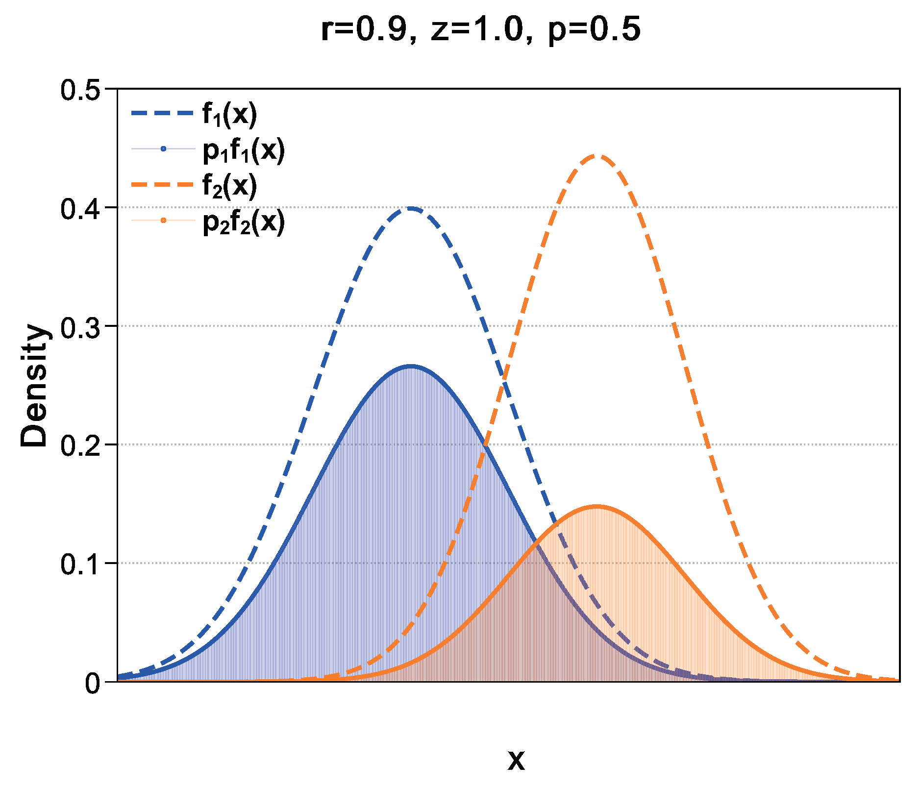
to make $b^2-4ac⩾0$. Figure 5 is a typical example for $f_1\left(x\right)$, $f_2\left(x\right)$, $p_1{f}_1\left(x\right)$, and $p_2{f}_2\left(x\right)$ with given $r,z,p$. In this example the $r,z,p$ fix Equation (15), so we have $p_2{f}_2\left(x\right)>p_1{f}_1\left(x\right)$ when $x_1<x<x_2$, where $x_1,x_2$ is the solution of Equation (12) and $x_1<x_2$. Let $f_1,f_2$ be $f_{T_i^{\ast }|s_1},f_{T_i^{\ast }|s_2}$, respectively, the privacy breaching method will match ${\mathbb{T}}^{\ast }(i,j^{\prime })$ to a ${\mathbb{S}}^{\ast }(i,l^{\prime })$ with value $s_2$ when ${\mathbb{T}}^{\ast }(i,j^{\prime })$ is in the interval $(x_1,x_2)$. If $r,z,p$ do not fix Equation (15), for example $p=0.1$, we have $p_2{f}_2\left(x\right)<p_1{f}_1\left(x\right)$ for any x, then the privacy breaching method will only match ${\mathbb{T}}^{\ast }(i,·)$ to the same value $s_1$ in ${\mathbb{S}}^{\ast }(i,·)$, which makes $s_2$ indistinguishable.

Figure 5. Schematic diagram of the probability density distribution of x when $r=0.9,z=1.0,$$p=0.5$. The horizontal coordinate axis is x, while the vertical coordinate axis is the probability density. Blue and orange dashed lines are curves of function $f_1\left(x\right)$ and $f_2\left(x\right)$, respectively, while the blue and orange solid lines are curves of function $p_1{f}_1\left(x\right)$ and $p_2{f}_2\left(x\right)$, respectively. The areas of the blue and orange regions are integrals of $f_1\left(x\right)$ and $f_2\left(x\right)$, respectively.

Next, we discuss how distinguishable $s_1$ and $s_2$ are. Let the area of the blue part be $A_b$, and the area of the orange part be $A_o$. It is obvious that $A_b=p_1,A_o=p_2$. The area where the blue part does not overlap with the orange part is $A_{b-o}$; similarly, the area where the orange part does not overlap with the blue part is $A_{o-b}$. As shown in Figure 5, the theoretical minimum error probability is given by the area under the minimum value of the two curves, which is the area of the overlapping area of blue and orange $A_{b\cap o}$.

For a given point x, the best theoretical error probability is given by the less likely one of the two classes:

$$\begin{array}{c}\hfill Pr\left(wrong\right|x)=min(p_1{f}_1\left(x\right),p_2{f}_2\left(x\right))\mathrm{d}x\end{array}$$

(16)

Then it can be integrated over the population to get the total error probability:

$$\begin{array}{c}\hfill A_{b\cap o}={\int }_{-\infty }^{+\infty }min(p_1{f}_1\left(x\right),p_2{f}_2\left(x\right))\mathrm{d}x\end{array}$$

(17)

According to Equation (17), we can obtain the area of $A_{b-o}$ and $A_{o-b}$ as

$$\begin{array}{c}\hfill A_{b-o}=A_b-A_{b\cap o}\\ \hfill A_{o-b}=A_o-A_{b\cap o}\end{array}$$

(18)

$A_{b-o}$, $A_{o-b}$ and $A_{b\cap o}$ are corresponding to important indicators in statistical analysis, where $A_{o-b}$ is true positive (TP), $A_{b-o}$ is true negative (TN), and $A_{b\cap o}$ is corresponding to both false positive (FP) and false negative (FN). Through these indicators we can use the relevant basic concepts of statistical analysis more directly, such as positive rate (TPR) or sensitivity, true negative rate (TNR) or speciality, and accuracy; the accuracy ${\mathrm{Acc}}^{\ast }$ and sensitivity ${\mathrm{Sen}}^{\ast }$ can be calculated as follows:

$$\begin{array}{cc}\hfill {\mathrm{Acc}}^{\ast }& =\frac{A_{b-o}+A_{o-b}}{A_{b-o}+A_{o-b}+2A_{b\cap o}}\hfill \\ \hfill {\mathrm{Sen}}^{\ast }& =\frac{A_{o-b}}{A_o}\hfill \end{array}$$

(19)

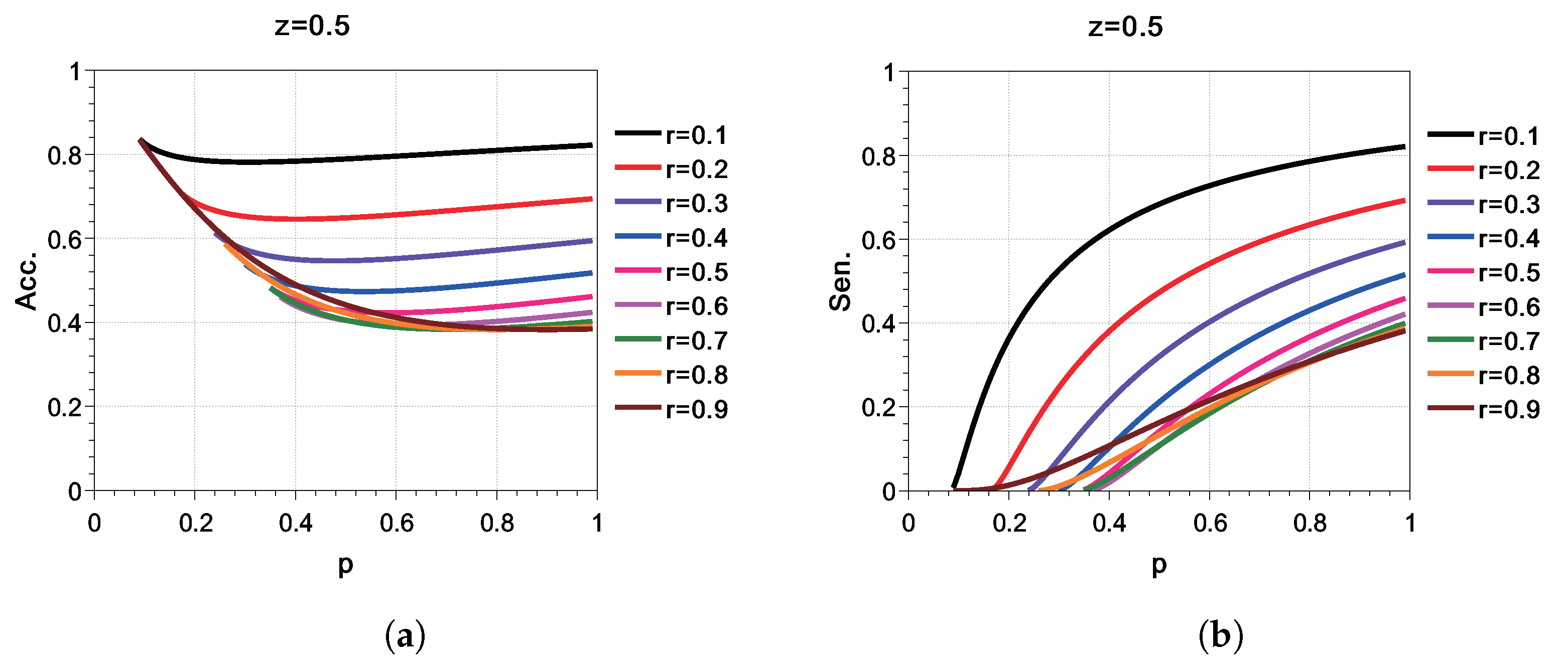
Substituting different $r,z,p$ combinations into Equation (19) shows that the accuracy and sensitivity are not positively correlated. Figure 6 is a typical example. Figure 6b shows that when $0<r<1,z=0.5$, the sensitivity decreases monotonically with the decrease of p. However, Figure 6a shows that with the same conditions, the accuracy does not decrease monotonically with the decrease of p: there are inflection points for each curve. When p becomes small enough, the accuracy will be very close to $100\%$, while the truncated curve means that $r,z,p$ do not fix Equation (15) if p is smaller than the breakpoint. In this situation, the sensitivity is 0.

Figure 6. Accuracyandsensitivityof binary classification with $z=0.5$. The horizontal coordinate axis is p, while the vertical coordinate axis is the value of accuracy and sensitivity. The curves represented by different r values are distinguished by different colors. (a) Accuracy. (b) Sensitivity.

The principle of privacy breaching attack is matching ${\mathbb{T}}^{\ast }(·,j^{\prime })$ to ${\mathbb{S}}^{\ast }(·,l^{\prime })$ with the highest average accuracy. If the sensitivity is too small (nearly 0) for matching most of the ${\mathbb{S}}^{\ast }(i,·)$ with ${\mathbb{T}}^{\ast }(i,·)$, the privacy breaching attack will match ${\mathbb{T}}^{\ast }(·,j^{\prime })$ to the same SNP profile with possibly high accuracy, which results in matching the vast majority ${\mathbb{T}}^{\ast }(·,j^{\prime })$ to an error ${\mathbb{S}}^{\ast }(·,l^{\prime })$. For a privacy breaching attack, it is more important to be able to distinguish ${\mathbb{S}}^{\ast }(·,l^{\prime })$ by ${\mathbb{T}}^{\ast }(·,j^{\prime })$, therefore the matching accuracy should be mainly related to sensitivity.

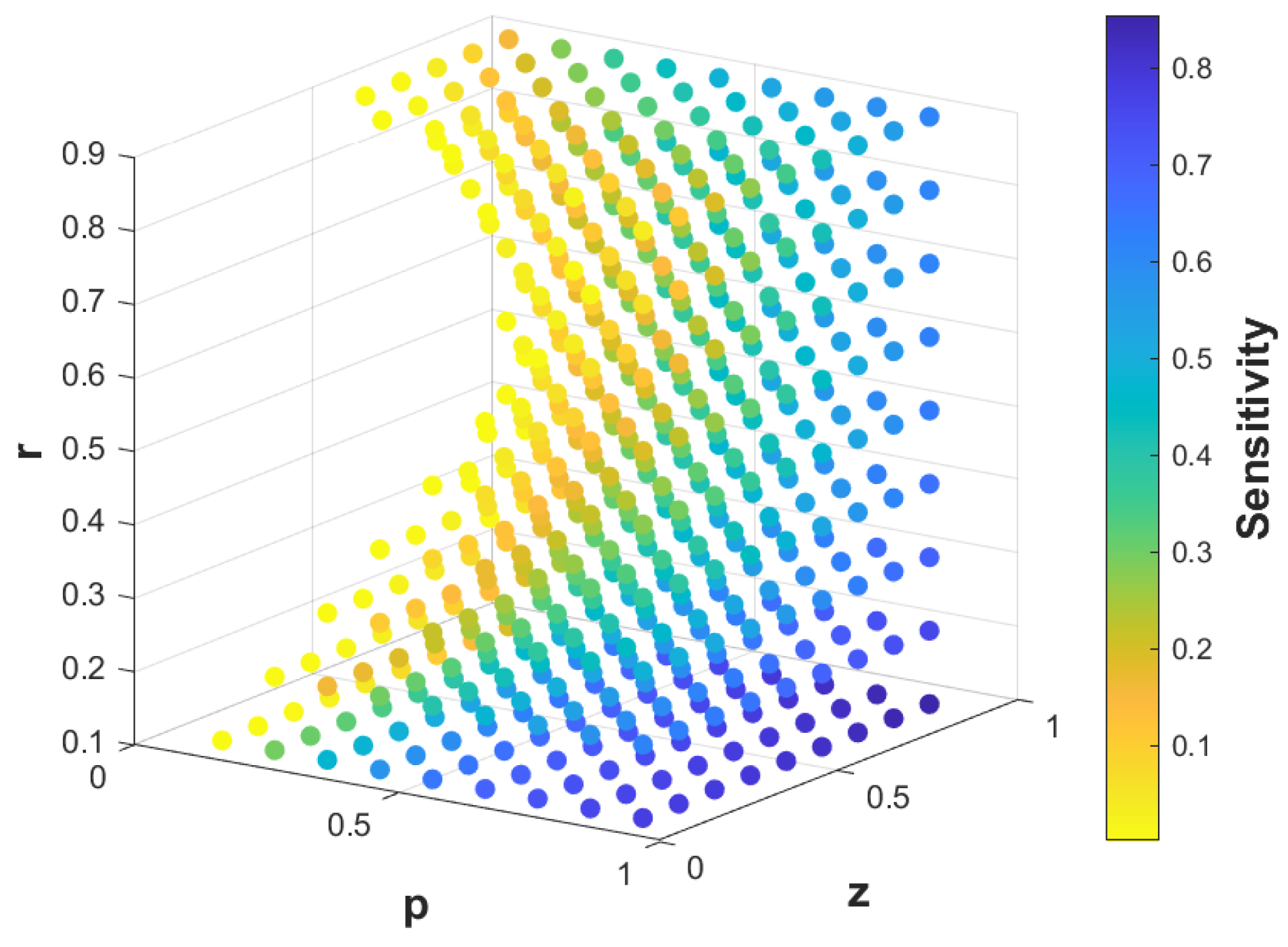
We test different r, z, and p in Equation (19) and found interesting correlations between these three parameters and sensitivity. Figure 7 shows the changing trend of sensitivity with $0<r<1$, $0<z<1$, and $0<p<1$ very intuitively. Empty positions indicate that the sensitivity there is 0. The boundary with the sensitivity of 0 is a saddle-shaped cambered surface. The sensitivity of the side of the cambered surface face to $p=0,z=0$ is 0; on the other side of the cambered surface, the farther away from the surface, the higher the sensitivity.

Figure 7. Sensitivitywith different r, z, and p. The three coordinates represent r, z, and p, respectively. Sensitivity is represented by different colors. The deeper the color, the higher the sensitivity. The vacant parts indicate that the sensitivity is zero when $r,z,p$ take the corresponding values.

6.3.2. Ternary SNP-Based Classification Analysis

Similarly with the derivation process for binary classification, let the prior probabilities of distributions $f_1\left(t\right)$, $f_2\left(t\right)$, and $f_3\left(t\right)$ be $p_1$, $p_2$, and $p_3$, respectively, then the intersection points t between joint distribution $p_1{f}_1\left(t\right)$, $p_2{f}_2\left(t\right)$ and $p_3{f}_3\left(t\right)$ can be represented as

$$\begin{array}{c}\hfill \frac{p_1}{\sqrt{2\pi }{\sigma }_1}exp(-\frac{{(t-{\mu }_1)}^2}{2{\sigma }_1^2})=\frac{p_2}{\sqrt{2\pi }{\sigma }_2}exp(-\frac{{(t-{\mu }_2)}^2}{2{\sigma }_2^2})\\ \hfill \frac{p_1}{\sqrt{2\pi }{\sigma }_1}exp(-\frac{{(t-{\mu }_1)}^2}{2{\sigma }_1^2})=\frac{p_3}{\sqrt{2\pi }{\sigma }_3}exp(-\frac{{(t-{\mu }_3)}^2}{2{\sigma }_3^2})\\ \hfill \frac{p_2}{\sqrt{2\pi }{\sigma }_2}exp(-\frac{{(t-{\mu }_2)}^2}{2{\sigma }_2^2})=\frac{p_3}{\sqrt{2\pi }{\sigma }_3}exp(-\frac{{(t-{\mu }_3)}^2}{2{\sigma }_3^2})\end{array}$$

(20)

Let $r_{\alpha }=\frac{{\sigma }_2}{{\sigma }_1},r_{\beta }=\frac{{\sigma }_3}{{\sigma }_1},r_{\gamma }=\frac{{\sigma }_3}{{\sigma }_2}$, then we have $r_{\gamma }=\frac{r_{\beta }}{r_{\alpha }}$. With MAF value $p_{\mathrm{m}}$ and the definition of MAF from Section 2.3, $p_1$, $p_2$, and $p_3$ can be represented as $p_1$$={(1-p_{\mathrm{m}})}^2$, $p_2=2p_{\mathrm{m}}(1-p_{\mathrm{m}})$, and $p_3=p_{\mathrm{m}}^2$. Let $p_{\alpha }=\frac{p_2}{p_1},p_{\beta }=\frac{p_3}{p_1},p_{\gamma }=\frac{p_3}{p_2}$, then we have $p_{\alpha }=\frac{2p_{\mathrm{m}}}{1-p_{\mathrm{m}}},p_{\beta }={\left(\frac{p_{\mathrm{m}}}{1-p_{\mathrm{m}}}\right)}^2,p_{\gamma }=\frac{p_{\mathrm{m}}}{2(1-p_{\mathrm{m}})}$. To simplify $p_{\alpha },p_{\beta },p_{\gamma }$, let $\frac{p_{\mathrm{m}}}{1-p_{\mathrm{m}}}=p_{\mathrm{st}}$, then we have $p_{\alpha }=2p_{\mathrm{st}},p_{\beta }=p_{\mathrm{st}}^2,p_{\gamma }=\frac{p_{\mathrm{st}}}{2}$. For the values of z, Let $z_{\alpha }=\frac{{\mu }_2-{\mu }_1}{{\sigma }_1+{\sigma }_2},z_{\beta }=\frac{{\mu }_3-{\mu }_1}{{\sigma }_1+{\sigma }_3},$$z_{\gamma }=\frac{{\mu }_3-{\mu }_2}{{\sigma }_2+{\sigma }_3}$, then $z_{\gamma }$ can be represented as $z_{\gamma }=\left[(1+r_{\beta })z_{\beta }-(1+r_{\alpha })z_{\alpha }\right]/\left(1+r_{\beta }/r_{\alpha }\right)$. Finally let $x=\frac{t-{\mu }_1}{{\sigma }_1}$, and substitute $r_{\alpha },r_{\beta },p_{\mathrm{st}},z_{\alpha },z_{\beta }$ into Equation (20), then we have three quadratic equations:

$$\begin{array}{cc}\hfill (r_{\alpha }^2-1)x^2+2(r_{\alpha }+1)z_{\alpha }x-[{(1+r_{\alpha })}^2{z}_{\alpha }^2+2r_{\alpha }^{2}ln\frac{r_{\alpha }}{2p_{\mathrm{st}}}]& =0\hfill \\ \hfill (r_{\beta }^2-1)x^2+2(r_{\beta }+1)z_{\beta }x-[{(1+r_{\beta })}^2{z}_{\beta }^2+2r_{\beta }^{2}ln\frac{r_{\beta }}{p_{\mathrm{st}}^2}]& =0\hfill \\ \hfill (\frac{r_{\beta }^2}{r_{\alpha }^2}-1)x^2+2[(1+r_{\beta })z_{\beta }-(1+r_{\alpha })z_{\alpha }]x& \\ \hfill -\{{[(1+r_{\beta })z_{\beta }-(1+r_{\alpha })z_{\alpha }]}^2+2\frac{r_{\beta }^2}{r_{\alpha }^2}ln\frac{2r_{\beta }}{p_{\mathrm{st}}{r}_{\alpha }}\}& =0\hfill \end{array}$$

(21)

Equation (21) shows that for each pair $\{{\mathbb{T}}^{\ast }(i,·),{\mathbb{S}}^{\ast }(i,·)\}$, there are three sensitivity values, which are determined by five parameters $z_{\alpha },z_{\beta },r_{\alpha },r_{\beta },p_{\mathrm{m}}$. Our synthetic data was generated without considering the factor r, hence $z_{\alpha },z_{\beta },p_{\mathrm{m}}$ of the synthetic data are pre-set while $r_{\alpha },r_{\beta }$ are random, which can explain the fluctuation of the matching accuracy in Figure 3. Figure 7 shows that a change in r will have a significant impact on sensitivity when the value of z is not high, while it has less effect on sensitivity if the value of z is high enough, which fix our matching accuracy results appropriately. Similarly, if $p_{\mathrm{m}}$ is low, $p_{\alpha },p_{\beta },p_{\gamma }$ will all be small values, resulting in a low sensitivity in most cases even $r_{\alpha },r_{\beta }$ are floating.

6.3.3. Sensitivity Score of Synthetic Data

We combine the results of binary classification to the case of ternary SNP-based classification. For i-th continuous trait with its most correlative SNP, we define its sensitivity score ${\mathrm{Sen}}_i$ as

$$\begin{array}{c}\hfill \mathrm{Sen}\left(i\right)=min\left(\mathrm{Sen}(i,·)\right)\end{array}$$

(22)

where $\mathrm{Sen}(i,·)$ is the sensitivity calculated by Equation (21) with pairwise combinations between $f_{Q_i|s_1},f_{Q_i|s_2},f_{Q_i|s_3}$ as $\{f_{Q_i|s_1},f_{Q_i|s_2}\}$, $\{f_{Q_i|s_1},f_{Q_i|s_3}\}$ and $\{f_{Q_i|s_2},f_{Q_i|s_3}\}$ from i-th continuous trait. Then the data sensitivity score $\mathrm{Sen}$ can be calculated as

$$\begin{array}{c}\hfill \mathrm{Sen}=\frac{1}{m}\sum _{i=1}^{m}min\left(\mathrm{Sen}(i,·)\right)\end{array}$$

(23)

We calculate the $\mathrm{Sen}$ of all our synthetic data. Typical results are shown in Figure 8. Similar to the conclusion that can be drawn from Figure 7, the larger the z, the higher the $\mathrm{Sen}$; the smaller the $p_{\mathrm{m}}$, the lower the $\mathrm{Sen}$. However, the sample size n can also influence $\mathrm{Sen}$. Data sensitivity score decreases as n increases when $p_{\mathrm{m}}$ is small ($p_{\mathrm{m}}=0.05,p_{\mathrm{m}}=0.15$); if $p_{\mathrm{m}}$ is large, the data sensitivity score is basically not affected by the change of n. The most likely reason is undersampling. If the sample size of synthetic data is small, undersampling is prone to occur for small $p_{\mathrm{m}}$, resulting in a falsely high data sensitivity score; as n increases, the probability of undersampling becomes lower, and the data sensitivity score is no longer artificially high. In contrast, datasets with $p_{\mathrm{m}}⩽0.30$ are not prone to undersampling when n is small, therefore the data sensitivity score is relatively stable. In addition, for our privacy breaching method, when the MAF value $p_{\mathrm{m}}$ is small, the increase of n mainly leads to a significant difference between the sensitivity of the matching set and the training set, which is also the main reason that the smaller the MAF, the more obvious the matching accuracy declines with the increase of n.

Figure 8. Sensitivity score$\mathrm{Sen}$ with SNP size $m=50$. The sample sizes n as 50, 100, 200, and 500 are expressed on the abscissa, respectively, while the matching accuracy is expressed on the ordinate. Matching accuracy with different MAFs and their standard deviations are expressed as different colored symbols with error bars, while the orange ellipse, red rectangle, olive diamond and blue triangle represent the MAF value of $0.05$, $0.15$, $0.30$ and $0.45$, respectively. (a,b) indicate z of $0.13$ and $2.33$, respectively. (a) $z=0.13$. (b) $z=2.33$.

Figure 8 also demonstrates the phenomenon that the ability to distinguish TP and FP matching by F score does not only correlate significantly with the data sensitivity score. Even though the value of the sensitivity score is up to $0.9$ as shown in Figure 8b with MAF value $p_{\mathrm{m}}=0.05$, it is still hard to find an effective threshold for distinguishing. It is speculated that the discrimination rate of TP and FP matching by F score is most positively correlated with the absolute value of $A_{0-b}$, or more precisely $E[\mathrm{Sen}(i,·)\times p_{\mathrm{m}}^2]$. Since the main factor affecting the value of $A_{0-b}$ is $p_{\mathrm{m}}^2$, the discrimination rate of TP and FP matching by F score is mainly related to $p_{\mathrm{m}}$.

6.3.4. Overall Analysis

From the experimental results and mathematical analysis above, to judge whether ${\mathbb{T}}^{\prime }(·,k^{\prime })$ in a continuous trait dataset ${\mathbb{T}}^{\prime }$ can effectively match a SNP sample ${\mathbb{S}}^{\prime }(·,l^{\prime })$, there are three major aspects as follows:

(a)

Both the SNP size m and the data sensitivity score of the QTL dataset ${\mathbb{T}}^{\prime }$ are most positively correlated with matching accuracy. The larger the m and data sensitivity score $\mathrm{Sen}$ related to the $r,z,p$ of each ${\mathbb{T}}^{\prime }(i,·)$, the higher the matching accuracy.

(b)

The discrimination rate of TP and FP matching between ${\mathbb{T}}^{\prime }$ and ${\mathbb{S}}^{\prime }$ by F score is most positively correlated with the MAF value $p_{\mathrm{m}}$ and will be affected by m to some extent. The larger the MAF, the easier to distinguish between TP and FP matching.

(c)

The sample size n significantly affects matching accuracy, especially when the MAF value is small. The larger n, the lower the matching accuracy.

The sample size n, the SNP size m, and the data sensitivity score $\mathrm{Sen}$ can be used to predict the approximate range of matching accuracy; m and MAF value $p_{\mathrm{m}}$ can be used to estimate the discrimination rate of TP and FP matching by F score. In the next subsection, we will verify the effectiveness of these three major aspects in predicting the privacy risk of a real QTL dataset.

6.4. Real Data

We use a real QTL dataset to verify the validity of major factors summarized in the previous Section 6.3.4. The real dataset CSF pQTL study in the Japanese population used in this study consists of proteomics and SNPs publicly available in the gene expression omnibus (GEO) database under references GSE83708, GSE83709 and GSE83710. GSE83708 represents the SNPs of 89 samples with genotyping Q17, GSE83709 represents the SNPs of 44 samples with genotyping Q35, and GSE83710 is the proteomic data of all 133 samples, which were collected between May 2010 and February 2014 at the National Center Hospital, National Center of Neurology and Psychiatry, Kodaira, Tokyo, Japan [48]. The entire dataset contains the relative fluorescence units (RFU) of the cerebrospinal fluid (CSF) levels of 1126 proteins in 133 subjects and 954,703 SNPs.

Analysis by previous researchers [48] revealed that a total of 421 cis and 25 trans SNP-protein pairs were significantly correlated at a false discovery rate (FDR) of less than 0.01 ($P_{nominal}<7.66\times {10}^{-9}$); cis-only analysis revealed an additional 580 significant cis SNP-protein pairs with an FDR < 0.01 ($P_{nominal}<2.13\times {10}^{-5}$). All the data can be downloaded from the National Center for Biotechnology Information (NCBI) database.

6.5. Privacy Risk Estimation

We keep only the most correlated SNP for each protomic trait, resulting in 62 pairs of continuous trait and SNP based on previous work [48]. The matching accuracy and standard deviation for these 62 pairs are shown in Table 1:

Table 1. Matching Accuracy (MA) and F score for Real Data Matching.

MA	MA Std	F score	F score Std
$0.2255$	$0.0385$	$1.8747$	$0.7421$

Even though there are strong correlations between traits and genotypes as $P_{nominal}$ measured, the matching accuracy is still very low, which shows that the matching accuracy is not necessarily positively correlated with the correlations between traits and SNPs measured by $P_{nominal}$.

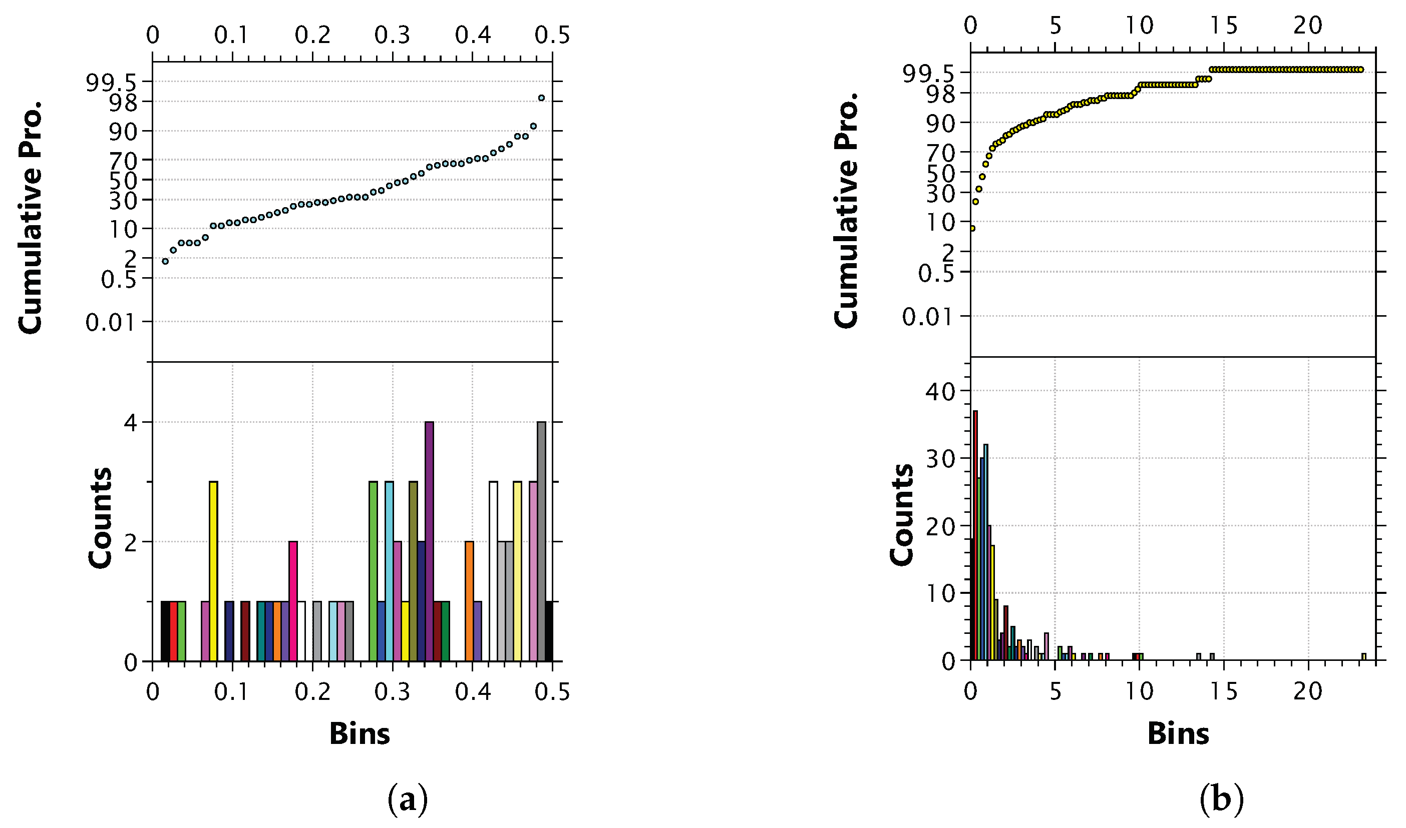
As Section 6.3.4 mentioned, there are three major aspects that affect matching accuracy and the discrimination rate of TP and FP matching. For the first major aspect, we calculate the data sensitivity score $\mathrm{Sen}$ of this real data and found it to be $0.2074$, which is close to the $\mathrm{Sen}$ of $z=0.13$ in Figure 8. The lower value of $\mathrm{Sen}$ is also consistent with condition that most of the z score (more than $70\%$) is low (less than $1.29$) as Figure 9b shows. The m of the real data is 62, which is close to the lowest m of our synthetic data. From the inference a in Section 6.3.4, low values of m and $\mathrm{Sen}$ will lead to low matching accuracy, and the actual matching accuracy from Table 1 shows that our inference is in line with the actual situation. For the second major aspect, it can be seen from Figure 9a that the MAF value $p_{\mathrm{m}}⩾0.30$ of nearly $70\%$ of the SNPs, so the discrimination rate between TP and FP matching should be high, which is also consistent with the results of F score in Table 1 (mostly upper than $1.0$). For the last major aspect, the n of the real data is 133, which is close to $n=100$ and means that the reliability needs to be improved. Combine these three aspects and match $m,n,z$ to where $m=50,n=100,z=0.13$ as shown in Figure 3, results show that there is a corresponding relationship between the matching accuracy of real data and synthetic data. Analysis of real data indicates that the three major aspects are effective in predicting privacy risk.

Figure 9. Counts and cumulative probability of the MAF values (a) and z scores (b) of the real data. The abscissa is the MAF values and z scores, the lower half of the ordinate is the number of MAFs/z scores in each interval of the histogram, and the upper half of the ordinate is the cumulative probability of each interval in the histogram. (a) MAF analysis. (b) $z_{\alpha }$ and $z_{\beta }$ analysis.

7. Discussion

The quantitative analysis we have proposed is not only for the possibility of privacy threats, but more importantly, for the probability of privacy risks for continuous trait data. Based on our findings from Section 6, we can classify the privacy risk by predicting the matching accuracy of the continuous trait data, so as to maximize the benefits of data sharing under the premise of ensuring data privacy. For example, we can divide the privacy risks of the continuous trait dataset into low, medium and high levels through the sensitivity score ($\mathrm{Sen}⩽0.25,0.25<\mathrm{Sen}⩽0.50,\mathrm{Sen}>0.50$). For the low-level data, we can adopt the form of resource disclosure that continuous trait data resources can be used and shared at any time with just anonymized. For the medium-level data, we need to adopt the form of platform collaborative data sharing, which should be based entirely on the sharing platform for cooperation; data should only be circulated and shared through the platform, while the shared data should not flow out of the collaborative data platform. For the high-level data, we must adopt the method of peer-to-peer data cooperation and adopt the cooperation principle of one discussion for one case. The cooperation application should include the description of both parties, the basis of cooperation, the purpose of cooperation, the mode of cooperation, the results of cooperation and the purpose of use, etc. In addition, the data provider also needs to add as much noise as possible to the trait data under the premise of ensuring availability according to the purpose of the cooperation.

Considering the influence of other factors, m, $p_{\mathrm{m}}$ and n are required to make corrections to the privacy risks. If $m⩽200$, the privacy risks will be increased by one level base on $\mathrm{Sen}$; similarly, if the proportion of SNPs with MAF value $p_{\mathrm{m}}<0.25$ in QTLs is greater than $50\%$, the privacy risks will be lowered by one level. Furthermore, if the QTL sample size is lower than 100, the privacy risks of the dataset should be preset to only medium and high levels.

8. Conclusions

We have presented a re-identification attack via simulated genotype data and showed that the matching SNP size is one of the major factors that can be used to quantify both genomic privacy breaching accuracy and the discrimination rate of TP and FP matching.

Then, by implementing a mathematical analysis of the distribution characteristics of our synthetic data, we demonstrated that the sensitivity, which is the main factor affecting the matching accuracy, is dependent on the ratio of standard deviation, the relative distance of expectation, and the ratio of prior probability, between different distributions with the same trait. Different from sensitivity, the MAF value is the main factor affecting the discrimination rate. Additionally, the size of the matching set will significantly affect the evaluation accuracy of privacy concerns in practical situations.

Finally, a matching test with real data led to the conclusion that our evaluation criteria are effective in predicting the privacy risks of gene-related continuous trait data.

Although our approach to assessing the privacy implications of continuous trait datasets has been shown to be effective, the present study has the following limitations, which need to be addressed in future studies.

First, the parameter setting of the simulated data needs to be more refined. Ratios between standard deviation $r_{\alpha }$ and $r_{\beta }$ should be more specific. Furthermore, since the distributions of $r_{\alpha }$ and $r_{\beta }$ were not specified when the data had been generated, the matching accuracy in Figure 2 and Figure 3 did not decrease monotonically with the increase of n and z but fluctuates, which was more likely to be related to the random distribution of $r_{\alpha }$ and $r_{\beta }$. For the further studies, we will focus on analyzing how different r will affect the sensitivity score and the effectiveness of the privacy breaching.

Second, sampling method for synthetic data generation needs to be improved. 50 times for sampling and training is inability to show hidden dangers accurately when faced with smaller MAFs. In the following studies we will increase the number of samples and increase the sample size of the training set. Furthermore, we will expand the value range of parameters to know under what conditions the privacy breaching attack can achieve the effect of the real data used in the prevous work [20,21].

Finally, the method of calculating the sensitivity score $\mathrm{Sen}\left(i\right)$ that for the ternary classification needs to be improved. The existing solution only considers the impact of the lowest $\mathrm{Sen}$ on the matching accuracy, but in actual cases, the impact of the second lowest $\mathrm{Sen}$ needs to be validated. In future studies we will estimate the impact of the second lowest $\mathrm{Sen}$ with more refined parameter settings.

References

- The International HapMap Consortium. The international HapMap project. Nature 2003, 426, 789. [Google Scholar] [CrossRef]
- Todorovic, V. Publisher Correction: Amplification-free single-cell whole-genome sequencing gets a makeover. Nat. Methods 2020, 17, 242. [Google Scholar] [CrossRef] [PubMed]
- Lappalainen, T.; Scott, A.J.; Brandt, M.; Hall, I.M. Genomic analysis in the age of human genome sequencing. Cell 2019, 177, 70–84. [Google Scholar] [CrossRef] [PubMed]
- Gawad, C.; Koh, W.; Quake, S.R. Single-cell genome sequencing: Current state of the science. Nat. Rev. Genet. 2016, 17, 175. [Google Scholar] [CrossRef] [PubMed]
- Bush, W.S.; Moore, J.H. Genome-wide association studies. PLoS Comput. Biol. 2012, 8, e1002822. [Google Scholar] [CrossRef] [PubMed]
- Chen, G.; Wang, C.; Shi, T. Overview of available methods for diverse RNA-Seq data analyses. Sci. China Life Sci. 2011, 54, 8. [Google Scholar] [CrossRef] [PubMed][Green Version]
- Genome-Wide Association Studies. Available online: https://www.mgi-tech.com/applications/info/8/ (accessed on 1 January 2020).
- 23 and Me Research Innovation Collaborations Program. Available online: https://research.23andme.com/research-innovation-collaborations/ (accessed on 1 January 2020).
- Kraft, P.; Haiman, C.A. GWAS identifies a common breast cancer risk allele among BRCA1 carriers. Nat. Genet. 2010, 42, 819–820. [Google Scholar] [CrossRef]
- Fachal, L.; Dunning, A.M. From candidate gene studies to GWAS and post-GWAS analyses in breast cancer. Curr. Opin. Genet. Dev. 2015, 30, 32–41. [Google Scholar] [CrossRef]
- Wang, X.F.; Zhou, X.; Rao, J.H.; Zhang, Z.J.; Yang, Y.D. Imputing DNA Methylation by Transferred Learning Based Neural Network. J. Comput. Sci. Technol. 2022, 37, 320–329. [Google Scholar] [CrossRef]
- Shi, Y.; Shao, S.; Zhang, X.; Wang, Y.; Wu, Y. Error exponent for concatenated codes in DNA data storage under substitution errors. Sci. China Inf. Sci. 2022, 65, 159304. [Google Scholar] [CrossRef]
- Fowler, J.H.; Settle, J.E.; Christakis, N.A. Correlated genotypes in friendship networks. Proc. Natl. Acad. Sci. USA 2011, 108, 1993–1997. [Google Scholar] [CrossRef] [PubMed]
- Humbert, M.; Ayday, E.; Hubaux, J.P.; Telenti, A. Addressing the concerns of the lacks family: Quantification of kin genomic privacy. In Proceedings of the ACM Sigsac Conference on Computer and Communications Security, Berlin, Germany, 4–8 November 2013. [Google Scholar]
- DNA Profiles from Ancestry Websites Helped Identify the Golden State Killer Suspect. Available online: https://www.vox.com/2018/4/27/17290288/golden-state-killer-joseph-james-deangelo-dna-profile-match (accessed on 1 January 2018).
- Greshake, B.; Bayer, P.E.; Rausch, H.; Reda, J. openSNP—A crowdsourced web resource for personal genomics. PLoS ONE 2014, 9, e89204. [Google Scholar] [CrossRef] [PubMed]
- Ball, M.P.; Bobe, J.R.; Chou, M.F.; Clegg, T.; Estep, P.W.; Lunshof, J.E.; Vandewege, W.; Zaranek, A.W.; Church, G.M. Harvard Personal Genome Project: Lessons from participatory public research. Genome Med. 2014, 6, 10. [Google Scholar] [CrossRef] [PubMed]
- Scaraglino, P. Complying with HIPAA: A guide for the university and its counsel. J. Coll. Univ. Law 2002, 29, 525. [Google Scholar]
- GenomePrivacy. Available online: https://genomeprivacy.org/ (accessed on 1 January 2021).
- Schadt, E.E.; Woo, S.; Hao, K. Bayesian method to predict individual SNP genotypes from gene expression data. Nat. Genet. 2012, 44, 603–608. [Google Scholar] [CrossRef]
- Backes, M.; Berrang, P.; Bieg, M.; Eils, R.; Herrmann, C.; Humbert, M.; Lehmann, I. Identifying personal DNA methylation profiles by genotype inference. In Proceedings of the 2017 IEEE Symposium on Security and Privacy (SP), San Jose, CA, USA, 22–26 May 2017; pp. 957–976. [Google Scholar]
- Sero, D.; Zaidi, A.; Li, J.; White, J.D.; Zarzar, T.B.G.; Marazita, M.L.; Weinberg, S.M.; Suetens, P.; Vandermeulen, D.; Wagner, J.K.; et al. Facial recognition from DNA using face-to-DNA classifiers. Nat. Commun. 2019, 10, 2557. [Google Scholar] [CrossRef]
- Lippert, C.; Sabatini, R.; Maher, M.C.; Kang, E.Y.; Lee, S.; Arikan, O.; Harley, A.; Bernal, A.; Garst, P.; Lavrenko, V.; et al. Identification of individuals by trait prediction using whole-genome sequencing data. Proc. Natl. Acad. Sci. USA 2017, 114, 10166–10171. [Google Scholar] [CrossRef]
- Jones, J. An introduction to factor analysis of information risk (fair). Norwich J. Inf. Assur. 2006, 2, 67. [Google Scholar]
- Kim, S.; Misra, A. SNP genotyping: Technologies and biomedical applications. Annu. Rev. Biomed. Eng. 2007, 9, 289–320. [Google Scholar] [CrossRef]
- Johnson, A.D.; O’Donnell, C.J. An Open Access Database of Genome-wide Association Results. BMC Med. Genet. 2009, 10, 6. [Google Scholar] [CrossRef]
- Liu, B.H. Statistical Genomics: Linkage, Mapping, and QTL Analysis; CRC Press: Boca Raton, FL, USA, 2017. [Google Scholar]
- Reay, W.R.; Atkins, J.R.; Carr, V.J.; Green, M.J.; Cairns, M.J. Pharmacological enrichment of polygenic risk for precision medicine in complex disorders. Sci. Rep. 2020, 10, 879. [Google Scholar] [CrossRef] [PubMed]
- Ng, B.; White, C.C.; Klein, H.U.; Sieberts, S.K.; McCabe, C.; Patrick, E.; Xu, J.; Yu, L.; Gaiteri, C.; Bennett, D.A.; et al. An xQTL map integrates the genetic architecture of the human brain’s transcriptome and epigenome. Nat. Neurosci. 2017, 20, 1418. [Google Scholar] [CrossRef] [PubMed]
- Gillespie, J.H. Population Genetics: A Concise Guide; JHU Press: Baltimore, MD, USA, 2004. [Google Scholar]
- Hernandez, R.D.; Uricchio, L.H.; Hartman, K.; Ye, C.; Dahl, A.; Zaitlen, N. Ultrarare variants drive substantial cis heritability of human gene expression. Nat. Genet. 2019, 51, 1349–1355. [Google Scholar] [CrossRef]
- Yaniv, E.; Arvind, N. Routes for breaching and protecting genetic privacy. Nat. Rev. Genet. 2014, 15, 409–421. [Google Scholar]
- Pakstis, A.J.; Speed, W.C.; Fang, R.; Hyland, F.C.; Furtado, M.R.; Kidd, J.R.; Kidd, K.K. SNPs for a universal individual identification panel. Hum. Genet. 2010, 127, 315–324. [Google Scholar] [CrossRef] [PubMed]
- Lin, Z.; Owen, A.B.; Altman, R.B. Genomic research and human subject privacy. Science 2004, 305, 183. [Google Scholar] [CrossRef]
- Beacon Network. Available online: https://beacon-network.org/ (accessed on 1 January 2018).
- Shringarpure, S.S.; Bustamante, C.D. Privacy risks from genomic data-sharing beacons. Am. J. Hum. Genet. 2015, 97, 631–646. [Google Scholar] [CrossRef]
- Hagestedt, I.; Zhang, Y.; Humbert, M.; Berrang, P.; Tang, H.; Wang, X.; Backes, M. MBeacon: Privacy-Preserving Beacons for DNA Methylation Data. In Proceedings of the Network and Distributed System Security Symposium, San Diego, CA, USA, 24–27 February 2019. [Google Scholar]
- Homer, N.; Szelinger, S.; Redman, M.; Duggan, D.; Tembe, W.; Muehling, J.; Pearson, J.V.; Stephan, D.A.; Nelson, S.F.; Craig, D.W. Resolving individuals contributing trace amounts of DNA to highly complex mixtures using high-density SNP genotyping microarrays. PLoS Genet. 2008, 4, e1000167. [Google Scholar] [CrossRef]
- Jacobs, K.B.; Yeager, M.; Wacholder, S.; Craig, D.; Kraft, P.; Hunter, D.J.; Paschal, J.; Manolio, T.A.; Tucker, M.; Hoover, R.N.; et al. A new statistic and its power to infer membership in a genome-wide association study using genotype frequencies. Nat. Genet. 2009, 41, 1253–1257. [Google Scholar] [CrossRef]
- Visscher, P.M.; Hill, W.G. The limits of individual identification from sample allele frequencies: Theory and statistical analysis. PLoS Genet. 2009, 5, e1000628. [Google Scholar] [CrossRef]
- Sankararaman, S.; Obozinski, G.; Jordan, M.I.; Halperin, E. Genomic privacy and limits of individual detection in a pool. Nat. Genet. 2009, 41, 965–967. [Google Scholar] [CrossRef] [PubMed]
- Philibert, R.A.; Terry, N.; Erwin, C.; Philibert, W.J.; Beach, S.R.; Brody, G.H. Methylation array data can simultaneously identify individuals and convey protected health information: An unrecognized ethical concern. Clin. Epigenet. 2014, 6, 28. [Google Scholar] [CrossRef] [PubMed]
- Dyke, S.O.; Cheung, W.A.; Joly, Y.; Ammerpohl, O.; Lutsik, P.; Rothstein, M.A.; Caron, M.; Busche, S.; Bourque, G.; Rönnblom, L.; et al. Epigenome data release: A participant-centered approach to privacy protection. Genome Biol. 2015, 16, 142. [Google Scholar] [CrossRef] [PubMed]
- Venkatesaramani, R.; Malin, B.A.; Vorobeychik, Y. Re-identification of Individuals in Genomic Datasets Using Public Face Images. arXiv 2021, arXiv:2102.08557. [Google Scholar] [CrossRef]
- Gymrek, M.; McGuire, A.L.; Golan, D.; Halperin, E.; Erlich, Y. Identifying personal genomes by surname inference. Science 2013, 339, 321–324. [Google Scholar] [CrossRef]
- Backes, M.; Berrang, P.; Humbert, M.; Shen, X.; Wolf, V. Simulating the large-scale erosion of genomic privacy over time. IEEE/ACM Trans. Comput. Biol. Bioinform. 2018, 15, 1405–1412. [Google Scholar] [CrossRef]
- Berrang, P.; Humbert, M.; Zhang, Y.; Lehmann, I.; Eils, R.; Backes, M. Dissecting privacy risks in biomedical data. In Proceedings of the 2018 IEEE European Symposium on Security and Privacy (EuroS&P), London, UK, 24–26 April 2018; pp. 62–76. [Google Scholar]
- Sasayama, D.; Hattori, K.; Ogawa, S.; Yokota, Y.; Matsumura, R.; Teraishi, T.; Hori, H.; Ota, M.; Yoshida, S.; Kunugi, H. Genome-wide quantitative trait loci mapping of the human cerebrospinal fluid proteome. Hum. Mol. Genet. 2016, 26, 44–51. [Google Scholar] [CrossRef]
- Humbert, M.; Huguenin, K.; Hugonot, J.; Ayday, E.; Hubaux, J.P. De-anonymizing genomic databases using phenotypic traits. Proc. Priv. Enhancing Technol. 2015, 2015, 99–114. [Google Scholar] [CrossRef]
- Deciphering the Map of RNA Modifications from Epitranscriptome Sequencing Data. Available online: https://rna.sysu.edu.cn/rmbase/ (accessed on 1 January 2018).
- dbSNP. Available online: https://www.ncbi.nlm.nih.gov/SNP/ (accessed on 1 January 2018).
- Ramos, E.M.; Din-Lovinescu, C.; Bookman, E.B.; McNeil, L.J.; Baker, C.C.; Godynskiy, G.; Harris, E.L.; Lehner, T.; McKeon, C.; Moss, J.; et al. A mechanism for controlled access to GWAS data: Experience of the GAIN Data Access Committee. Am. J. Hum. Genet. 2013, 92, 479–488. [Google Scholar] [CrossRef]
- He, M.; Zou, D.; Qiang, W.; Wu, W.; Xu, S.; Deng, X.; Jin, H. Utility-Prioritized Differential Privacy for Quantitative Biomedical Data. J. Circuits, Syst. Comput. 2022, 31, 2250236. [Google Scholar] [CrossRef]
- Fienberg, S.E.; Slavkovic, A.; Uhler, C. Privacy preserving GWAS data sharing. In Proceedings of the 2011 IEEE 11th International Conference on Data Mining Workshops, Vancouver, BC, Canada, 11 December 2011; pp. 628–635. [Google Scholar]
Publisher’s Note: MDPI stays neutral with regard to jurisdictional claims in published maps and institutional affiliations. |
© 2022 by the authors. Licensee MDPI, Basel, Switzerland. This article is an open access article distributed under the terms and conditions of the Creative Commons Attribution (CC BY) license (https://creativecommons.org/licenses/by/4.0/).