CloudRCNN: A Framework Based on Deep Neural Networks for Semantic Segmentation of Satellite Cloud Images

Abstract

Shadow cumulus clouds are widely distributed globally. They carry critical information to analyze environmental and climate changes. They can also shape the energy and water cycles of the global ecosystem at multiple scales by impacting solar radiation transfer and precipitation. Satellite images are an important source of cloud data. The accurate detection and segmentation of clouds is of great significance for climate and environmental monitoring. In this paper, we propose an improved MaskRCNN framework for the semantic segmentation of satellite images. We also explore two deep neural network architectures using auxiliary loss and feature fusion functions. We conduct comparative experiments on the dataset called “Understanding Clouds from Satellite Images”, sourced from the Kaggle competition. Compared to the baseline model, MaskRCNN, the mIoU of the CloudRCNN (auxiliary loss) model improves by 15.24%, and that of the CloudRCNN (feature fusion) model improves by 12.77%. More importantly, the two neural network architectures proposed in this paper can be widely applied to various semantic segmentation neural network models to improve the distinction between the foreground and the background.

1. Introduction

Climate change has been impacting increasingly both the environment and human activities. Continuously monitoring the dynamic change of Earth’s climate, temporally and spatially, has attracted significant efforts. Clouds are the most uncertain but important factor in Earth’s climate system. According to the Global Energy and Water Cycle Experiment Cloud Assessment Dataset, the global average cloud coverage is about 68% per year [1,2]. By affecting solar radiation transfer and precipitation, clouds can shape the energy and water cycles of the global ecosystem at multiple scales. Therefore, investigating the shape of clouds will facilitate the study of the climate of the corresponding region.

The accurate detection and segmentation of clouds is of great significance for identifying different weather systems, for meteorological forecasting, and for preventing natural disasters. Meteorological satellites can observe the cloud coverage on Earth from top to bottom. Satellite images are an important source of cloud data. The semantic segmentation of clouds is a challenging task during the processing of satellite cloud images.

Over the years, multiple classes of methods have been developed for image segmentation. The threshold-based image segmentation method [3,4,5] classifies image pixel points into several classes by setting different feature thresholds. The superpixel-based image segmentation method [6,7] aggregates neighboring pixels with similar texture, color, luminance, and other features into a certain block of pixels to achieve the purpose of replacing a large number of pixels with a small number of blocks. Watershed-based image segmentation methods [8,9] use similarity between neighboring pixels as an important reference, so that pixels with similar spatial locations and similar grayscale values are connected to form a closed contour. Level-set-based image segmentation methods [10,11] use a numerical technique for interface tracking and shaping a geometric activity profile model. However, traditional machine learning-based image segmentation methods have difficulty meeting the demand for highly accurate, robust, and portable methods. In recent years, deep learning-based image segmentation methods have made great breakthroughs and have gained the attention of researchers. Many excellent models and architectures have been widely applied in visual recognition systems and have achieved great results, including satellite remote sensing image detection, medical image analysis, video surveillance, etc.

There are various solutions proposed for the semantic segmentation of satellite cloud images. However, most of them are based on the direct enhancement of features, such as using attention mechanisms [12] and stronger backbones to enrich the semantic information; they do not take advantage of the fact that clouds are easily distinguished from the background, while there is little difference between different types of clouds.

In this paper, we propose an improved MaskRCNN [13] framework for the semantic segmentation of satellite images. We design a deconvolution decoder composed of a parallel convolution block and a spatial attention deconvolution block. The deconvolution decoder is used to extract the binary semantic segmentation mask results that distinguish the foreground and the background, thereby suppressing the output of false-positive masks, refining the boundary information of semantic segmentation, and improving the pixel-wise accuracy of the semantic segmentation of the satellite cloud layer. We also explore two architectures of deep neural networks that use auxiliary loss and feature fusion, and conduct comparative experiments on the dataset called “Understanding Clouds from Satellite Images” [14] from the Kaggle competition. More importantly, the two neural network architectures proposed in this paper can be widely applied to various semantic segmentation neural network models to improve the distinction between the foreground and the background.

Instead of using Kaggle’s board as the evaluation metrics, which are used by another paper [15] with the same dataset, we use mIoU (mean intersection-over-union) as the evaluation metric because the scoring mechanism of Kaggle’s board is not public, making it difficult to analyze the experimental results reasonably. Compared with the performance of the baseline MaskRCNN model, the mIoU of the CloudRCNN (auxiliary loss) model improves by 15.22%, and that of the CloudRCNN (feature fusion) model improves by 13.57%. The main contributions of this research are listed as follows:

• We propose two designs to improve MaskRCNN according to the characteristics in the satellite cloud images (the clouds and the background can be easily distinguished while different types of clouds have little difference);
• We explore two branch designs of MaskRCNN, including using auxiliary loss to supervise the foreground and designing a feature fusion module to restore the feature map, so as to judge the feature extraction of the first-stage convolution;
• We design comprehensive experiments on the Kaggle competition dataset called “Understanding Clouds from Satellite Images” to evaluate the performance of our model, which achieves substantial improvements over MaskRCNN.

The rest of this paper is organized as follows. Section 2 reviews related research work. Section 3 explains our proposed model and dataset. In Section 4, comprehensive experiments are conducted to evaluate the effectiveness of the proposed model. Finally, in Section 5, we conclude the paper and provide future work.

2. Related Work

2.1. Deep Learning-Based Methods

Semantic segmentation methods based on deep learning are developing rapidly [16,17,18,19,20], and these methods are also applicable to the task of segmenting clouds in satellite images. Researchers have added different functional modules to the original network structure to improve the segmentation effect.

Dev et al. proposed CloudSegNet [21] for efficient cloud segmentation. As a lightweight deep learning architecture, it is the first general framework that deals with daytime and nighttime sky/cloud images in a single framework. The framework achieves great performance with a precision of 0.92, a recall value of 0.87, an F-score of 0.89, and an error rate of 0.08 on the composite dataset of SWIMSEG (Singapore Whole sky IMaging SEGmentation Dataset) and SWINSEG (Singapore Whole sky Nighttime IMaging SEGmentation Database).

Marc et al. proposed a modified U-Net-based method [22] for the semantic segmentation of clouds and cloud shadows in single-date images from various multispectral satellites without the need for retraining or human intervention. Based on comparative experiments on the globally distributed multi-sensor test dataset, this method consistently outperforms the state-of-the-art methods.

Guo et al. proposed Cloud-Attu [12] for cloud detection, which is a deep learning model based on U-Net. The Cloud-Attu model introduces an attention mechanism and adopts a symmetric encoder–decoder structure. Using skip-connection operation, the model is able to fuse high-level features with low-level features, which enriches the multi-scale information in the output results. The symmetric structure shows its great advantage in improving the segmentation of images. Based on comparative experimental results, the proposed model outperforms the traditional method in terms of accuracy, even with disturbances from bright non-cloud objects.

Xia et al. proposed a global attention feature fusion residual network [23] that aims to address the limitations of spectral bands and complex backgrounds in cloud segmentation. The proposed method can automatically classify clouds, shadows, and backgrounds. The model adopts a residual network [24] as the backbone for semantic information extraction and introduces an improved atrous spatial pyramid pooling method for handling boundary information. It also uses the global attention up-sample mechanism for information fusion and improves the utilization of global and local features. Through experiments, the model demonstrates great performance in cloud and shadow segmentation.

To address the limits of CNN-based cloud detection methods, Liu et al. proposed DCNet [25], a deformable convolutional cloud detection network. The proposed model is more adaptable to cloud variations. Deformable convolution blocks are introduced at the encoder and a skip connection mechanism is integrated into the decoder. The proposed method outperforms state-of-the-art models on GF-1 wide-field-of-view satellite images.

2.2. Multi-Task and Auxiliary Loss Supervised Semantic Segmentation Models

Multi-task learning has been successfully used in various applications of machine learning to help us obtain information we ignored previously and to help improve the metrics we care about [26]. One guise of multitask learning is the use of auxiliary loss.

Islam et al. designed a lightweight cascaded convolutional neural network [27] based on assisted supervised deep adversarial learning. It is designed for the real-time segmentation of robotic surgical instruments. A multi-resolution feature fusion (MFF) module is designed to aggregate feature maps from auxiliary and main branches. The method proposed in [27] combines auxiliary loss and adversarial loss model-regularization techniques. The model outperformed the previous best performance in every category of segmentation on the MICCAI Robotic Instrument Segmentation Challenge 2017, including binary segmentation, part segmentation, and instrument segmentation.

Zhang et al. proposed a semantic segmentation framework named ExFuse (Enhancing Feature Fusion for Semantic Segmentation) [28]. It improves the effectiveness of subsequent feature fusion by introducing semantic information and high-resolution details into low-level features and high-level features, respectively. The proposed method involves another module: semantic supervision (SS). This module directly assigns auxiliary supervision to the early stages of the encoder network. The framework achieved an 87.9% mIoU on Pascal VOC 2012, which outperformed the state-of-the-art results at the time.

Zheng et al. proposed an end-to-end network structure called GAMNet (Gate and Attention Modules Net) [29] for high-resolution image semantic segmentation. In this structure, an attention module is integrated with a gating module. It also designs a composite loss function, which adds an auxiliary loss to achieve deep supervision of GAM. Experiments were conducted on the ISPRS2-D semantic labeling datasets and the results showed that the performance of GAMNet was the best at the time.

Inception net [30], a deep convolutional neural network architecture, was proposed by Szegedy et al. It solves the vanishing gradient problem and provides regularization by adding auxiliary classifiers connected to intermediate layers. It enables an increase in the depth and width of the network without changing the computational budget. The Hebbian principle was followed during the design of the architecture to achieve better quality. The system achieved significantly better performance than the state-of-the-art models at the time in the ILSVRC 2014 classification and detection challenges.

Aslani et al. proposed a simple and effective multi-data source segmentation method for magnetic resonance imaging (MRI) [31]. They proposed a regularization network with an auxiliary loss term. It integrates regularization into the standard encoder–decoder network and effectively alleviates the domain shift problem. Compared to baseline models, the method demonstrated better generalization performance.

2.3. Semantic Segmentation Models Based on Feature Fusion Module

Deep neural networks compute features layer by layer, which leads to semantic gaps in features between different layers. Further, it makes it difficult for the detector to obtain specific-enough semantic information. Feature fusion methods have become the new focus, which can reduce the semantic gaps and fully exploit multi-scale features [32].

Cheng et al. proposed (AF)2-S3Net [33] for 3D LiDAR semantic segmentation. It is a CNN network with an end-to-end encoder–decoder. In the encoder, a novel multi-branch attentive feature fusion module is presented. In the decoder, a unique feature selection module is presented. Combining voxel-based learning and point-based learning, the proposed method demonstrates its advantage in the large 3D scene scenario. The proposed method ranked 1st on the large-scale SemantiKITTI benchmarks.

Irfan et al. proposed an ultrasound breast lesion image segmentation method based on a dilated semantic segmentation network (Di-CNN) [34]. Combined with morphological erosion operations, the proposed method includes a 24-layer CNN for feature extraction. It uses a parallel fusion method to fuse the feature map. The method outperformed other algorithms on the mask-based ultrasound imaging dataset and achieves an accuracy of 98.9%.

Shang et al. proposed an end-to-end multi-scale adaptive feature fusion network (MANET) [35] that addresses the challenge of the semantic segmentation of high-resolution remote sensing images. It involves a multi-scale context extraction module (MCM) and an adaptive fusion module (AFM). To fuse semantic features, it integrates a channel attention mechanism. It also generates global features by concatenating high-level semantic information and low-level semantic information. With experiments conducted on the Potsdam and Vaihingen datasets, the proposed MANET outperformed other existing networks, achieving an accuracy of 89.4% and 88.2%, and an average F1 of 90.4% and 86.7%, respectively.

Zhou et al. proposed a self-attention feature fusion network (SA-FFNet) [36] for semantic segmentation. A vertical and horizontal compression attention module (VH-CAM) is adopted into the network, as well as an unequal channel pyramid pooling module (UC-PPM). The feature map is compressed vertically and horizontally to achieve richer information in each pixel. It also improves the special feature map. Experiments are conducted on two datasets: PASCAL VOC2012 and Cityscapes; the proposed method outperformed other models with an mIoU of 76.42% and 73.13%, respectively.

2.4. Comparison of Our Model with Existing Models

We compare the strengths and weaknesses of the proposed research model and the three existing models mentioned before. MaskRCNN uses RPN (region proposal network) to obtain a series of candidate regions and classifies the image regions after feature extraction using a classifier. The strengths and weaknesses of MaskRCNN are listed as follows:

• Strengths:
  • Can generate candidate regions using object detection techniques, is capable of simultaneously performing object detection and image semantic segmentation tasks;
  • The ROI (region of interest) align layer is introduced to make the alignment of the feature map and the original image more accurate by bilinear interpolation.
• Weaknesses:
  • Insufficient consideration of global semantic information in the image;
  • It is easy to make mistakes when detecting small target objects.

Deeplab-v3 [18] is an improved full convolutional network. The strengths and weaknesses of Deeplab-v3 are listed as follows:

• Strengths:
  • The ASPP (atrous spatial pyramid pooling) module is introduced to increase the perceptual field of the network and reduce the loss of the feature image size;
  • Optimized edge segmentation by using a decoder to refine the segmentation results.
• Weaknesses:
  • Large computational volume and slow segmentation speed;
  • Less-accurate segmentation of small-scale objects.

GAMNet [29] introduces an attention module with a gating module and designs a composite loss function that adds an auxiliary loss to achieve deep supervision of GAM. The strengths and weaknesses of GAMNet are listed as follows:

• Strengths:
  • The introduction of the GAM module can improve the segmentation performance of small targets while imposing boundary constraints;
  • The designed compound loss function facilitates model optimization and improves the performance of integrated modules.
• Weaknesses:
  • Large computational volume and slow segmentation speed;
  • Shaded areas are easily misclassified on the ISPRS dataset.

CloudRCNN (our method) has improved on MaskRCNN and introduces feature fusion, a spatial attention module, and an auxiliary branch with a decoder structure. The strengths and weaknesses of CloudRCNN are listed as follows:

• Strengths:
  • The backbone of MaskRCNN is too long, which is prone to the gradient explosion problem. The auxiliary branch introduced by this model is a good correction of the problem;
  • The model performs additional focused segmentation on the subject of the input image, so the model segments the subject’s edges more carefully;
  • The introduced spatial attention module refines the boundary information for semantic segmentation.
• Weaknesses:
  • The number of pixels in the background is often larger than the segmented subject, and the additional supervision of foreground–background information causes the model to prefer to classify pixels as background.

3. Materials and Methods

3.1. Dataset

In this research, we use the dataset from the Kaggle competition (“Understanding Clouds from Satellite Images” [14]) which was held in November 2019. Competitors were required to identify regions in satellite cloud images with different cloud formations labeled as Fish, Flower, Gravel, and Sugar. Each image contains at least one formation and up to all four.

Through the crowd-sourcing platform Zooniverse, 10,000 satellite images were screened. Each image was labeled by at least three scientists from a team of 68 scientists. They identified cloud patterns in each image. About 50,000 medium-scale cloud organizations were identified. Lots of noises have been included in the labels in the dataset, and many regions do not even contain clouds. In addition, different types of cloud masks also overlap [37].

In this dataset, each image is labeled separately for the four categories: Fish, Flower, Gravel, and Sugar. Figure 1 shows example images of the four categories. One label is called a sample, and an image has four samples. If a cloud category does not exist in the image, the corresponding sample is empty. The dataset consists of 5546 images, with 4436 images in the training set and 1110 images in the test set. For the training set, there are 17,744 samples (4 × 4436) in total, and 8267 samples are empty. With empty samples being removed, 9477 samples remain. Similarly, for the test set, there are 4440 samples (4 × 1110) in total, and 2081 samples are empty, so there are 2359 available samples.

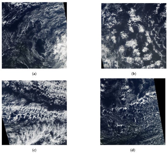
Figure 1. Samples of the four cloud categories: Sugar, Flower, Fish, and Gravel. (a) Sugar; (b) Flower; (c) Fish; (d) Gravel.

Table 1 shows the basics of the dataset, including the training set and the test set.

Table 1. Dataset basics.

Training Set (9477 Samples)
Category	Sample	Percentage
Fish pattern	2219	23.41%
Flower pattern	1881	19.94%
Gravel pattern	2341	24.70%
Sugar pattern	3036	32.04%
Testing Set (2359 Samples)
Category	Sample	Percentage
Fish pattern	2219	23.82%
Flower pattern	1881	20.52%
Gravel pattern	2341	25.36%
Sugar pattern	3036	30.31%

3.2. System Architecture

In this research, we propose two architectures for the semantic segmentation of clouds: CloudRCNN (auxiliary loss) and CloudRCNN (feature fusion). Both architectures are based on MaskRCNN, and we add an auxiliary branch to enhance model performance. Figure 2 shows the system architecture of CloudRCNN (auxiliary loss) and CloudRCNN (feature fusion). For both architectures, satellite images are fed into MaskRCNN for semantic segmentation. The C4 layer feature map of ResNet is used as the input for the auxiliary branch. For CloudRCNN (auxiliary loss), as shown in Figure 2a, the auxiliary branch is a deconvolution decoder, and the feature map obtained by the decoder will be used to supervise the foreground and the background information. For CloudRCNN (feature fusion), as shown in Figure 2b, the auxiliary branch consists of a deconvolution decoder and a feature extraction network based on ResNet and FPN [38]. The feature map obtained by this branch will be used for feature fusion in the form of element-wise multiplication with the feature map of the backbone network of MaskRCNN.

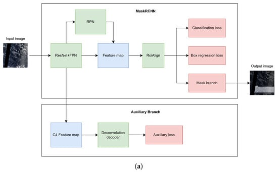
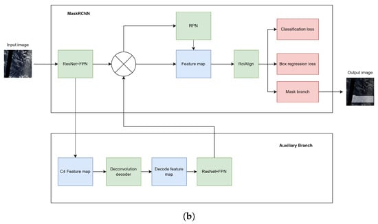
Figure 2. The architecture of the two designs. (a) The architecture of CloudRCNN (auxiliary loss); (b) The architecture of CloudRCNN (feature fusion).

3.3. Methods

3.3.1. Spatial Attention Module

Many studies have shown that introducing attention mechanisms into neural networks can improve the ability of network models to express features. The spatial attention module from CBAM (convolutional block attention module) [39] is a kind of effective attention mechanism which indicates the importance of the input values in the spatial dimension. It has been used in many applications due to its ease of integration. Figure 3 shows the details of the spatial attention module. The implementation of spatial attention is to perform MaxPool and AvgPool in the channel dimension to obtain two 2D spatial feature maps that capture cross-channel information. The feature map contains position-sensitive feature information. We use a 7 × 7 convolution kernel to fuse the feature map information of MaxPool and AvgPool and use the sigmoid function to make the value of each point in the feature map between 0–1, which indicates the probability that the pixel is foreground or background. Finally, an element-wise dot product with the input feature map is conducted to suppress the feature of the background. The spatial attention module allows the model to locate and identify target regions more accurately. The computation is explained in Formulas (1) and (2).

$$\sigma (x)=\frac{1}{1-e^{(-x)}}$$

(1)

$$M_s(F)=F⨂(\sigma (f^{7\times 7}([AvgPool(F);MaxPool(F)])))$$

(2)

F represents the input feature map and $F^{\prime }$ represents the output feature map. $M_s$ represents the feature map through the attention module. ⨂ stands for element-wise multiplication. $\sigma$ represents the sigmoid activation function. $f^{n\times n}$ represents a convolutional layer with a convolution kernel of n, with the size of the input and output feature maps unchanged. $Avgpool$ stands for average pooling, and $MaxPool$ stands for max pooling.

Figure 3. Spatial attention module.

3.3.2. Spatial Attention Deconvolution Block

Figure 4 shows the architecture of the spatial attention deconvolution block. We integrate the spatial attention module and design the spatial attention deconvolution block. In the spatial attention deconvolution block, we connect the input feature map and the obtained attention feature map for residual connection, then feed it into the deconvolution module. In this way, we achieve both the fusion of the feature map information and up-sampling. Finally, batch normalization and a ReLU activation function is introduced to generate the output feature map of the spatial attention deconvolution block. The computation is explained in Formulas (3) and (4).

$$Relu(x)=max(0,x)$$

(3)

$$F^{\prime }=Relu(Bn(f_T^{3\times 3}(F⨁M_s(F))))$$

(4)

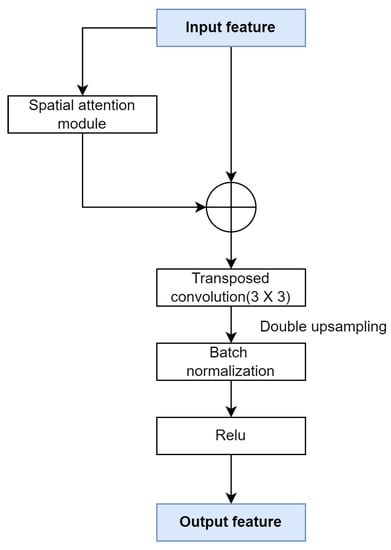
Figure 4. Spatial attention deconvolution block.

F represents the input feature map and $F^{\prime }$ represents the output feature map. $M_s$ represents the feature map through the attention module. ⨁ stands for element-wise addition. $f_T^{n\times n}$ represents a convolution kernel of n and a stride of 2, which is used for a transposed convolution layer with 2-times up-sampling. $Bn$ stands for ratio normalization. $Relu$ stands for the ReLU activation function.

3.3.3. Parallel Convolution Block

Figure 5 shows the design of the parallel convolution block. It is designed based on the inception module in [30]. Convolution kernels of different sizes are utilized to obtain different sizes of receptive fields. The inception module splices the convolution kernel sizes of 1 × 1, 3 × 3, and 5 × 5 in parallel, which requires huge computing resources. After comprehensively considering the number of parameters and the computation complexity, in the design of the parallel convolution block, we feed the feature map into a convolution layer with a convolution kernel size of 1 × 1, as well as a convolution layer with a convolution kernel size of 3 × 3, in parallel. In this way, the network is more adaptive to different cloud scales. The output feature maps are then added element-wise, which fuses the features at different scales. Finally, the result is fed into a transposed convolutional layer with a kernel size of 3 × 3, so that each layer of the model captures image information in various forms, such as low-level edges, intermediate-level edge connections, high-level object parts, and complete objects. The computation of the parallel convolution block is defined by Formula (5).

$$F^{\prime }=Relu(Bn(f_T^{3\times 3}(f^{1\times 1}(F)⨁f^{3\times 3}(F))))$$

(5)

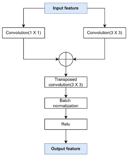
Figure 5. Parallel convolution block.

3.3.4. Deconvolution Decoder

Figure 6 shows the architecture of the deconvolution decoder. The design of the deconvolution decoder is based on the ResNet structure [24]. Properly stacking the network can extract more complex feature patterns. Our deconvolution decoder network consists of four stages. Each stage is composed of a parallel convolution block and a spatial attention deconvolution block. Each stage will extract deep-level features and up-sample the feature map by a factor of 2. The feature map of the ResNet C4 layer is fed into the network. After the decoder, a feature map with the same size as the original image is obtained.

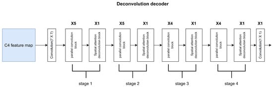
Figure 6. Deconvolution decoder.

3.3.5. The Auxiliary Branch in CloudRCNN (Auxiliary Loss)

The design of the auxiliary branch in CloudRCNN (auxiliary loss) is shown in Figure 7.

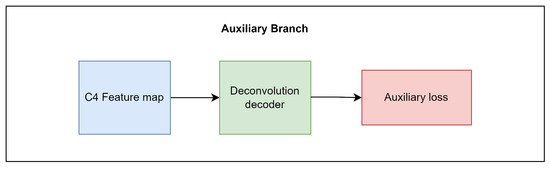
Figure 7. The auxiliary branch of CloudRCNN (auxiliary loss).

In satellite cloud images, the foreground is easily differentiated from the background, while clouds look similar. Based on this characteristic, we design the auxiliary branch to additionally supervise the foreground and the background. We reconstruct all the ground truths in the dataset when we supervise the auxiliary branch. We set the pixels in the non-background to be 1, and set the pixels in the background to be 0, which builds up the ground truth of the binary classification of each image with only foreground and background, subsequently enhancing the distinction between the foreground and the background as well. The deconvolution decoder is the main component of the auxiliary branch. After the deconvolution decoder, the resolution of the feature map will be the same as the input image, and the pixel-by-pixel cross-entropy loss $L_{aux}$ can be calculated. Stochastic gradient descent is used for backpropagation of the loss during training.

The computation is explained in Formulas (6)–(8).

$$L=L_{maskrcnn}+L_{aux};$$

(6)

$$L_{maskrcnn}=L_{mask}+L_{cls}+L_{box};$$

(7)

$$L_{aux}=\frac{1}{N}\sum -(y_i\times log(p_i)+(1-y_i)\times log(1-p_i))$$

(8)

$L_{maskrcnn}$ is the loss function of MaskRCNN. $L_{aux}$ is an auxiliary loss function, used to additionally supervise the foreground and background using a cross-entropy loss function, where $y_i$ represents the label of pixel i, the foreground is 1, and the background is 0. $p_i$ represents the probability that the pixel is predicted to be the foreground.

3.3.6. The Feature Fusion of CloudRCNN (Feature Fusion)

The design of the feature fusion in CloudRCNN (feature fusion) is shown in Figure 8.

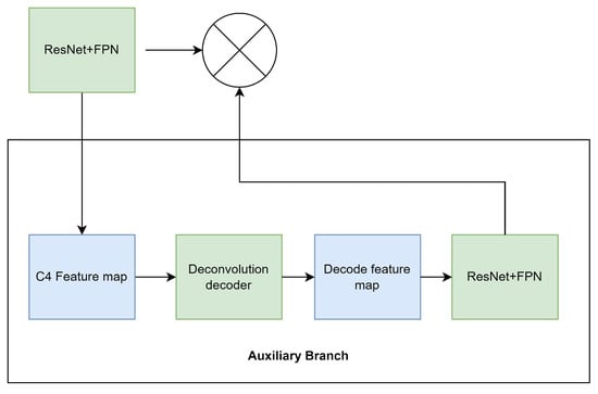
Figure 8. The feature fusion design of CloudRCNN (feature fusion).

The deconvolution decoder is also included in the feature fusion design and has the same structure as the decoder in Figure 6. The input feature map is also the C4 feature map of ResNet. To reduce the computational complexity of the network, we halved the number of channels of ResNet on both the backbone network and the branch; the feature map from the decoder then becomes the input of the ResNet with FPN in the auxiliary branch. Finally, we perform the element-wise multiplication of the feature map output by the FPN in the backbone network and the feature map output by the FPN from the auxiliary branch, which achieves the feature fusion. This corrects the feature map roughly extracted in the first stage. We also use the fused feature map for subsequent forward propagation. The computation is explained in Formula (9).

$$F_i^{\prime }=F_i⨂F{D}_i,i\in [2,6]$$

(9)

$F^{\prime }$ represents the feature map after feature fusion. F represents the feature map fed into the auxiliary branch, which is generated by ResNet with FPN on the backbone network. $FD$ represents the feature map generated by ResNet with FPN on the auxiliary branch. ⨂ stands for element-wise multiplication.

4. Experiments and Results

To evaluate the effectiveness of our proposed models, we designed comparative experiments on a computer with an Intel(R) Xeon(R) CPU E5-2630 v3 @ 2.40 GHz, equipped with GeForce GTX 1080, and running Ubuntu 20.04.2 LTS. Our experiments were designed in Python. The main Python libraries that we used are Tensorflow and Keras. We also used Matterport’s MaskRCNN framework [40] to build our models. The dataset has 5546 images in total, of which 4436 images are the training set and 1110 images are the test set. The training set contains 9477 samples and the test set has 2359 samples.

4.1. Evaluation Metric

We use the mean intersection-over-union (mIoU) as the evaluation metric, which is commonly used in semantic segmentation tasks. In our experiments, we calculate the ratio of the intersection and the union of the two sets of the true pixel-by-pixel classification results and the predicted pixel-by-pixel classification results. The ratio indicates the accuracy of the segmentation results. The computation is explained in Formula (10).

$$mIoU=\frac{1}{k+1}\sum _{i=0}^k\frac{p_{ij}}{{\sum }_{j=0}^k{p}_{ij}+{\sum }_{j=0}^k{p}_{ji}-p_{ii}}$$

(10)

where k represents the number of categories of the prediction task (excluding the background), $p_{ij}$ represents the pixel whose true value is i and is predicted to be j, and $p_{ii}$ is the correctly predicted pixel. $p_{ij}$ and $p_{ji}$ represent the pixels predicted to be false positives and false negatives, respectively.

4.2. Baseline Model

We chose MaskRCNN as the baseline model. MaskRCNN achieves top results in the COCO suite of challenges and outperformed the winners of the COCO2016 Challenge [13]. MaskRCNN is a classic two-stage object instance segmentation algorithm model, which is improved from FasterRCNN. The first stage includes the backbone network, feature pyramid networks (FPN), and region proposal networks (RPN). The second stage consists of a region-of-interest alignment module and three parallel branches, namely, a bounding box regression branch for object detection tasks, a bounding box classification branch, and a pixel-wise classification branch for semantic segmentation tasks. Figure 9 shows the main components of MaskRCNN.

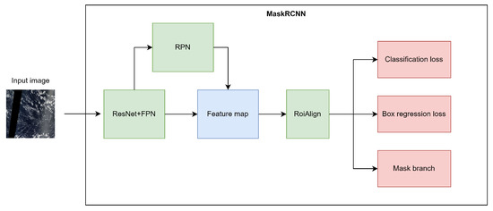
Figure 9. MaskRCNN: two-stage object instance segmentation neural network.

4.3. Model Training

For experiments, we trained the models with 50 epochs. The image size was set to be 512. The learning rate for MaskRCNN was 0.00000001, and the learning rate for both CloudRCNN (auxiliary loss) and CloudRCNN (feature fusion) was 0.0001. The learning momentum for all three models was 0.9. The batch size aas 1 and the optimizer was stochastic gradient descent.

4.4. Comparative Results

The quantitative results of this experiment are shown in Table 2. In this experiment, MaskRCNN [13] was set as the basic model. From the Table 2, it can be found that both CloudRCNN (auxiliary loss) and CloudRCNN (feature fusion) demonstrate better performance than the baseline MaskRCNN model in every category. This proves the effectiveness of the two CloudRCNNs we designed. Compared with MaskRCNN, the mIoU of CloudRCNN (auxiliary loss) improves by 15.24%, and that of CloudRCNN (feature fusion) improves by 12.77%. We chose two other state-of-the-art models for comparison experiments with our models, including PointRend [19] and SCNet [20]. For each subclass, CloudRCNN (auxiliary loss) achieved the best results for the Flower and Gravel categories, CloudRCNN (feature fusion) achieved the best results for the Sugar category, and SCNet achieved the best results for the Fish category. In terms of mIoU, CloudRCNN (auxiliary loss) achieves the best mIoU among all models listed in Table 2. The experimental results show that our approaches outperform the baseline model and other advanced models and achieve state-of-the-art results with this dataset.

Table 2. Comparative results of five models.

Model	Fish	Flower	Gravel	Sugar	mIoU
MaskRCNN	0.2830	0.1991	0.2458	0.3171	0.2613
PointRend	0.3728	0.2816	0.4123	0.4254	0.3746
SCNet	0.3953	0.3177	0.4769	0.3984	0.4019
CloudRCNN (auxiliary loss)	0.3813	0.3288	0.5246	0.4202	0.4137
CloudRCNN (feature fusion)	0.3520	0.2769	0.4668	0.4601	0.3890

Figure 10 shows two sets of comparative results of MaskRCNN, PointRend, SCNet, CloudRCNN (auxiliary loss), and CloudRCNN (feature fusion). Two example satellite cloud images of Gravel and Sugar clouds are demonstrated. For the example of the Gravel-type cloud (Image 061cda5), MaskRCNN generates a false-positive semantic segmentation mask, and both the auxiliary and feature fusion models provide correct predictions, which indicates that the additional supervision of the background in our design enables the model to distinguish the foreground and the background better. Both PointRend and SCNet do not output a mask for false positives. For the case of the Sugar-type cloud (Image 0ad0a05), MaskRCNN and SCNet wrap more irrelevant background areas, and PointRend appears to have a large area of missed detection. At the same time, the auxiliary and feature fusion versions provide results closer to the ground truth results. This indicates that our spatial attention deconvolution block and parallel convolution block can sufficiently extract information from the target object region and collect cloud features from this information, thus distinguishing background classes and cloud classes to a greater extent and making the semantic segmentation results much more accurate.

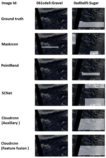
Figure 10. Two satellite images and the segmentation results of three models.

4.5. Error Discussion

According to the experiments in Section 4.4, we demonstrated the effectiveness of the spatial attention deconvolution block, the parallel convolution block, and two different design approaches for CloudRCNN. By comparing with other representative methods, it is proved that CloudRCNN can achieve more accurate semantic segmentations of satellite cloud images, with the benefit of combining the spatial attention module and the auxiliary branch, which improves the segmentation performance of the foreground and background. Even though CloudRCNN achieves a state-of-the-art semantic segmentation performance on the datasets [14], it still has several typical errors that need to be further corrected.

4.5.1. Misdetection Error

A misdetection case of a Flower-type cloud (Image 156f6aa) is shown in Figure 11. As shown in Figure 11, MaskRCNN generates a partially correct prediction mask, but CloudRCNN (auxiliary) considers that there is no flower-like cloud in the image. The misdetection may be due to the class imbalance between the background and foreground. Our model performs additional supervision on the foreground and background. With more pixels in the background than in the foreground in the dataset, the model will be more inclined to predict pixels as background classes.

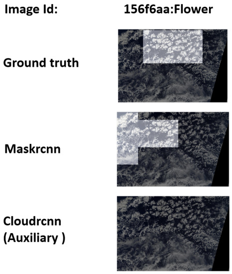
Figure 11. Misdetection example.

4.5.2. Label Errors

The datasets used in the study were annotated by a crowdsourcing platform. Some pixels were mislabeled in the ground truth, which would lead to incorrect predictions of the model. An example from the dataset is shown in Figure 12, where the background marked by a red circle is mislabeled as the cloud.

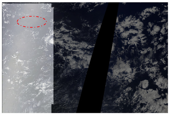
Figure 12. Label error example.

5. Conclusions

Shallow cumulus clouds are widely distributed globally. They are sensitive to changes in the environment and have great potential to affect the radiation balance on Earth. The results of semantic segmentations of clouds play a vital role in cloud observations and forecasts, due to their real-time nature and their accuracy. With cloud-cover information, we can update the weather information on time to monitor climate changes, identify different weather systems, and prevent natural disasters such as tornadoes, storms, hail, and floods.

The existing research in this field does not fully utilize the feature that the characteristics of clouds and backgrounds are very different, while the characteristics of different types of clouds are small. In this research, we design neural networks to explore this feature. We propose a semantic segmentation method according to the four cloud categories in satellite cloud images. We design our models based on MaskRCNN, which is also our baseline model. We add a deconvolution decoder to extract the binary classification message to distinguish the foreground and the background, suppress the output of false-positive masks, refine the boundary information of semantic segmentation, and improve the pixel-wise accuracy of semantic segmentations of satellite cloud images. The deconvolution decoder is composed of parallel convolution blocks and a spatial attention deconvolution block. We also explore two designs of neural network structures using auxiliary loss and feature fusion and compare their performance on the dataset “Understanding Clouds from Satellite Images”. Compared to the baseline MaskRCNN model, the mIoU of CloudRCNN (auxiliary loss) improves by 15.24%, and that of CloudRCNN (feature fusion) improves by 12.77%.

Meanwhile, this research has some limitations, which will be addressed in future work. Firstly, the dataset used in this research is from the crowdsourcing platform, roughly labeled, and a part of the background is labeled as clouds. The presence of these mislabeled noise labels can cause the network to optimize in the wrong direction, reducing the robustness of the network. We plan to adopt the noise transition matrix heuristically, or the “co-teaching” learning paradigm, to solve this problem. Secondly, the auxiliary branch brings with it complex calculations and more parameters, affecting real-time performance significantly when compared to other lightweight models. We plan to apply some pruning methods or knowledge distillation methods to the model to reduce its computational complexity and improve the real-time capability of satellite cloud segmentation. Thirdly, the labeling of satellite images is challenging and time-consuming. In the future, we could design a semi-supervised method and introduce the same type of unlabeled data to achieve the augmentation of datasets such as the 95-Cloud dataset and the SPARCS dataset, which will further improve the classification performance of the model. Fourth, we mainly validate our model by experimental design, which is deficient in theoretical analysis. In future work, we will carry out work related to model interpretability. Fifth, the number of pixels in the background is often larger than the segmented subject. The loss function can be redesigned and found to solve the class imbalance between foreground and background.

References

- King, M.D.; Platnick, S.; Menzel, W.P.; Ackerman, S.A.; Hubanks, P.A. Spatial and temporal distribution of clouds observed by modis onboard the terra and aqua satellites. IEEE Trans. Geosci. Remote Sens. 2013, 51, 3826–3852. [Google Scholar] [CrossRef]
- Sun, L.; Yang, X.; Jia, S.; Jia, C.; Wang, Q.; Liu, X.; Wei, J.; Zhou, X. Satellite data cloud detection using deep learning supported by hyperspectral data. Int. J. Remote Sens. 2020, 41, 1349–1371. [Google Scholar] [CrossRef] [Green Version]
- Otsu, N. A threshold selection method from gray-level histograms. IEEE Trans. Syst. Man Cybern. 1979, 9, 62–66. [Google Scholar] [CrossRef] [Green Version]
- Chen, S.; Chen, X.; Chen, J.; Jia, P.; Cao, X.; Liu, C. An iterative haze optimized transformation for automatic cloud/haze detection of landsat imagery. IEEE Trans. Geosci. Remote Sens. 2015, 54, 2682–2694. [Google Scholar] [CrossRef]
- Sun, L.; Mi, X.; Wei, J.; Wang, J.; Tian, X.; Yu, H.; Gan, P. A cloud detection algorithm-generating method for remote sensing data at visible to short-wave infrared wavelengths. ISPRS J. Photogramm. Remote Sens. 2017, 124, 70–88. [Google Scholar] [CrossRef]
- Lang, F.; Yang, J.; Yan, S.; Qin, F. Superpixel segmentation of polarimetric synthetic aperture radar (sar) images based on generalized mean shift. Remote Sens. 2018, 10, 1592. [Google Scholar] [CrossRef] [Green Version]
- Stutz, D.; Hermans, A.; Leibe, B. Superpixels: An evaluation of the state-of-the-art. Comput. Vis. Image Underst. 2018, 166, 1–27. [Google Scholar] [CrossRef] [Green Version]
- Ciecholewski, M. Automated coronal hole segmentation from solar euv images using the watershed transform. J. Vis. Commun. Image Represent. 2015, 33, 203–218. [Google Scholar] [CrossRef]
- Cousty, J.; Bertrand, G.; Najman, L.; Couprie, M. Watershed cuts: Thinnings, shortest path forests, and topological watersheds. IEEE Trans. Pattern Anal. Mach. Intell. 2009, 32, 925–939. [Google Scholar] [CrossRef] [Green Version]
- Braga, A.M.; Marques, R.C.; Rodrigues, F.A.; Medeiros, F.N. A median regularized level set for hierarchical segmentation of sar images. IEEE Geosci. Remote Sens. Lett. 2017, 14, 1171–1175. [Google Scholar] [CrossRef]
- Jin, R.; Yin, J.; Zhou, W.; Yang, J. Level set segmentation algorithm for high-resolution polarimetric sar images based on a heterogeneous clutter model. IEEE J. Sel. Top. Appl. Earth Obs. Remote Sens. 2017, 10, 4565–4579. [Google Scholar] [CrossRef]
- Guo, Y.; Cao, X.; Liu, B.; Gao, M. Cloud detection for satellite imagery using attention-based u-net convolutional neural network. Symmetry 2020, 12, 1056. [Google Scholar] [CrossRef]
- He, K.; Gkioxari, G.; Dollár, P.; Girshick, R. Mask r-cnn. In Proceedings of the IEEE International Conference on Computer Vision, Venice, Italy, 22–29 October 2017; pp. 2961–2969. [Google Scholar]
- Understanding Clouds from Satellite Images. Available online: https://www.kaggle.com/c/understanding_cloud_organization (accessed on 1 June 2021).
- Ahmed, T.; Sabab, N.H.N. Classification and understanding of cloud structures via satellite images with efficientunet. SN Comput. Sci. 2022, 3, 1–11. [Google Scholar] [CrossRef]
- Long, J.; Shelhamer, E.; Darrell, T. Fully convolutional networks for semantic segmentation. In Proceedings of the IEEE Conference on Computer Vision and Pattern Recognition, Boston, MA, USA, 7–12 June 2015; pp. 3431–3440. [Google Scholar]
- Ronneberger, O.; Fischer, P.; Brox, T. U-net: Convolutional networks for biomedical image segmentation. In International Conference on Medical Image Computing and Computer-Assisted Intervention; Springer: Cham, Switzerland, 2015; pp. 234–241. [Google Scholar]
- Chen, L.-C.; Zhu, Y.; Papandreou, G.; Schroff, F.; Adam, H. Encoder-decoder with atrous separable convolution for semantic image segmentation. In Proceedings of the European Conference on Computer Vision (ECCV), Munich, Germany, 8–14 September 2018; pp. 801–818. [Google Scholar]
- Kirillov, A.; Wu, Y.; He, K.; Girshick, R. Pointrend: Image segmentation as rendering. In Proceedings of the IEEE/CVF Conference on Computer Vision and Pattern Recognition, Seattle, WA, USA, 13–19 June 2020; pp. 9799–9808. [Google Scholar]
- Vu, T.; Haeyong, K.; Yoo, C.D. Scnet: Training inference sample consistency for instance segmentation. In Proceedings of the AAAI, Virtually, 2–9 February 2021. [Google Scholar]
- Dev, S.; Nautiyal, A.; Lee, Y.H.; Winkler, S. Cloudsegnet: A deep network for nychthemeron cloud image segmentation. IEEE Geosci. Remote Sens. Lett. 2019, 16, 1814–1818. [Google Scholar] [CrossRef] [Green Version]
- Wieland, M.; Li, Y.; Martinis, S. Multi-sensor cloud and cloud shadow segmentation with a convolutional neural network. Remote Sens. Environ. 2019, 230, 111203. [Google Scholar] [CrossRef]
- Xia, M.; Wang, T.; Zhang, Y.; Liu, J.; Xu, Y. Cloud/shadow segmentation based on global attention feature fusion residual network for remote sensing imagery. Int. J. Remote Sens. 2021, 42, 2022–2045. [Google Scholar] [CrossRef]
- He, K.; Zhang, X.; Ren, S.; Sun, J. Deep residual learning for image recognition. In Proceedings of the IEEE Conference on Computer Vision and Pattern Recognition, Las Vegas, NV, USA, 26 June–1 July 2016; pp. 770–778. [Google Scholar]
- Liu, Y.; Wang, W.; Li, Q.; Min, M.; Yao, Z. Dcnet: A deformable convolutional cloud detection network for remote sensing imagery. IEEE Geosci. Remote Sens. Lett. 2021, 19, 1–5. [Google Scholar] [CrossRef]
- Ruder, S. An overview of multi-task learning in deep neural networks. arXiv 2017, arXiv:1706.05098. [Google Scholar]
- Islam, M.; Atputharuban, D.A.; Ramesh, R.; Ren, H. Real-time instrument segmentation in robotic surgery using auxiliary supervised deep adversarial learning. IEEE Robot. Autom. Lett. 2019, 4, 2188–2195. [Google Scholar] [CrossRef]
- Zhang, Z.; Zhang, X.; Peng, C.; Xue, X.; Sun, J. Exfuse: Enhancing feature fusion for semantic segmentation. In Proceedings of the European Conference on Computer Vision (ECCV), Munich, Germany, 8–14 September 2018; pp. 269–284. [Google Scholar]
- Zheng, Z.; Zhang, X.; Xiao, P.; Li, Z. Integrating gate and attention modules for high-resolution image semantic segmentation. IEEE J. Sel. Top. Appl. Earth Obs. Remote Sens. 2021, 14, 4530–4546. [Google Scholar] [CrossRef]
- Szegedy, C.; Liu, W.; Jia, Y.; Sermanet, P.; Reed, S.; Anguelov, D.; Erhan, D.; Vanhoucke, V.; Rabinovich, A. Going deeper with convolutions. In Proceedings of the IEEE Conference on Computer Vision and Pattern Recognition, Boston, MA, USA, 7–12 June 2015; pp. 1–9. [Google Scholar]
- Aslani, S.; Murino, V.; Dayan, M.; Tam, R.; Sona, D.; Hamarneh, G. Scanner invariant multiple sclerosis lesion segmentation from mri. In Proceedings of the 2020 IEEE 17th International Symposium on Biomedical Imaging (ISBI), Iowa City, IA, USA, 3–7 April 2020; pp. 781–785. [Google Scholar]
- Deng, J.; Bei, S.; Shaojing, S.; Zhen, Z. Feature fusion methods in deep-learning generic object detection: A survey. In Proceedings of the 2020 IEEE 9th Joint International Information Technology and Artificial Intelligence Conference (ITAIC), Chongqing, China, 17–19 June 2020; Volume 9, pp. 431–437. [Google Scholar]
- Cheng, R.; Razani, R.; Taghavi, E.; Li, E.; Liu, B. 2-s3net: Attentive feature fusion with adaptive feature selection for sparse semantic segmentation network. In Proceedings of the IEEE/CVF Conference on Computer Vision and Pattern Recognition, Nashville, TN, USA, 20–25 June 2021; pp. 12547–12556. [Google Scholar]
- Irfan, R.; Almazroi, A.A.; Rauf, H.T.; Damaševičius, R.; Nasr, E.A.; Abdelgawad, A.E. Dilated semantic segmentation for breast ultrasonic lesion detection using parallel feature fusion. Diagnostics 2021, 11, 1212. [Google Scholar] [CrossRef] [PubMed]
- Shang, R.; Zhang, J.; Jiao, L.; Li, Y.; Marturi, N.; Stolkin, R. Multi-scale adaptive feature fusion network for semantic segmentation in remote sensing images. Remote Sens. 2020, 12, 872. [Google Scholar] [CrossRef] [Green Version]
- Zhou, Z.; Zhou, Y.; Wang, D.; Mu, J.; Zhou, H. Self-attention feature fusion network for semantic segmentation. Neurocomputing 2021, 453, 50–59. [Google Scholar] [CrossRef]
- Rasp, S.; Schulz, H.; Bony, S.; Stevens, B. Combining crowdsourcing and deep learning to explore the mesoscale organization of shallow convection. Bull. Am. Meteorol. Soc. 2020, 101, E1980–E1995. [Google Scholar]
- Lin, T.-Y.; Dollár, P.; Girshick, R.; He, K.; Hariharan, B.; Belongie, S. Feature pyramid networks for object detection. In Proceedings of the IEEE Conference on Computer Vision and Pattern Recognition, Honolulu, HI, USA, 21–26 July 2017; pp. 2117–2125. [Google Scholar]
- Woo, S.; Park, J.; Lee, J.-Y.; Kweon, I.S. Cbam: Convolutional block attention module. In Proceedings of the European Conference on Computer Vision (ECCV), Munich, Germany, 8–14 September 2018; pp. 3–19. [Google Scholar]
- Abdulla, W. Mask r-Cnn for Object Detection and Instance Segmentation on Keras and Tensorflow. 2017. Available online: https://github.com/matterport/Mask_RCNN (accessed on 2 August 2021).
Publisher’s Note: MDPI stays neutral with regard to jurisdictional claims in published maps and institutional affiliations. |
© 2022 by the authors. Licensee MDPI, Basel, Switzerland. This article is an open access article distributed under the terms and conditions of the Creative Commons Attribution (CC BY) license (https://creativecommons.org/licenses/by/4.0/).