Method for Select Best AIS Data in Prediction Vessel Movements and Route Estimation

Abstract

The prediction of vessel maritime navigation has become an exciting topic in the last years, especially considering economics, commercial exchange, and security. In addition, vessel monitoring requires better systems and techniques that help enterprises and governments to protect their interests. Specifically, the prediction of vessel movements is essential for safety and tracking. However, the applications of prediction techniques have a high cost related to computational efficiency and low resource saving. This article presents a sample method to select historical data on vessel-specific routes to optimize the computational performance of the prediction of vessel positions and route estimation in real-time. These historical navigation data can help to estimate a complete path and perform vessel position predictions through time. This Select Best AIS Data in Prediction Vessel Movements and Route Estimation (PreMovEst) method works in a Vessel Traffic Service database to save computational resources when predictions or route estimations are executed. This article discusses AIS data and the artificial neural network. This work aims to present a prediction model that correctly predicts the physical movement in the route. It supports path planning for the Vessel Traffic Service. After testing the method, the results obtained for route estimation have a precision of 76.15%, and those for vessel position predictions through time have an accuracy of 81.043%.

1. Introduction

Maritime navigation is an essential part of international trade. Global maritime exchange increased exponentially in 2017 [1], mainly driven by Asia and Europe’s economies since many countries export products around the world in large volumes. At the beginning of 2018, the merchant fleet was estimated to be 58,329 vessels [1], which led to more commercial exchange. It has also led to the amount of maritime traffic increasing, thus it is necessary to analyze the information to improve the monitoring processes for different purposes. Naval navigation has experienced a boom. One main task is monitoring the seas to describe and predict moving through them, and, since e-commerce is growing exponentially, vessels are the primary mode of transport for products. Today, governments and enterprises are more interested in it. Data mining techniques (e.g., [2]) aim to discover patterns of movement of the ships from the delimitation of an area.

Statistical analysis and clustering techniques are used. The principles of vessels with similar properties and association rules are used to analyze the movement of the ships and have been implemented to improve the maritime description such as classification, clustering, and predictions [3]. Moreover, where transit routes have been established for navigation, the knowledge of vessel positioning’s historical data allows for the predictive analysis. There are different ways to interpret the information generated, for maritime traffic, density, route estimation, and arrival times.

Likewise, to find vessel movements and prevent incidents, techniques such as maritime tracking and vessel monitoring systems have been proposed. For the latter, in 2002, the International Maritime Organization (IMO) approved the Automatic Identification System (AIS), which has now become an indispensable tool in terms of safety and vessel monitoring around the world.

The vessel industry is volatile, and so commerce and the carriers collaborate and cooperate in alliances. The industry is characterized by having very different freight rates depending on the direction of the trip. Several carriers should deliver the products in several journeys based on the origin country and destination. In 2020, with the COVID-19 pandemic, the number of vessels carrying goods to satisfy client demand has been growing a lot.

The origin and destination of vessels imply costs related to the physical routes; however, the costs should be reduced by selecting the optimal routes.

Besides, to ensure driver adherence to routes and other requirements for the vessel, there should always be a degree of maneuverability in cases that the real time ocean conditions cause changes to origins, destinations, and physical routes.

A vessel can use specific routes many times based on its origin and destination concerning historical vessel positions. Sometimes ships have to change course for different reasons such as adverse climatic agents, political disputes, or prohibitions; however, their trajectories are similar.

Vessel traffic services save historical records to have evidence of the vessel’s location. Industries such as marine traffic, whose system manages large amounts of navigational information for nearly 800 million position records per month, are an example of this.

We define route as the vessel trajectory from the departure port to the arrival port. The position is one set of the coordinates in time of the vessel. The series of positions is all trajectory points of one vessel. Speed is the vessel’s velocity. Course means the direction of the vessel’s grades.

One of the principal goals is the prediction and route estimation of vessel movements. It is a difficult task, however, because systems require high-performance computing. In addition, it requires historical information that can describe patterns in the flow of vessels.

The inferential statistic has generated a significant number of tools to contribute to making scientific judgments on the uncertainty data. Besides, localization measures are designed to provide quantitative values of the central location of the sample. These values will be helpful to identify differences between several of the vessel’s routes. This paper proposes an approach to data selection to reduce computational cost. This work does not focus on precision, but it shows a precision of 76.15% and an accuracy of 81.043% for vessel position predictions through time.

The paper is organized as follows. Section 2 shows a brief description of the related works. Section 3 describes the PreMovEst method for selecting the best AIS data in predicting vessel movements. Section 4 presents preliminary experiments to show the data behavior and adjust the data before selection. Section 5 describes the operations of selecting routes by clustering using the best statistical values. Section 6 presents the results of the experiments. Section 7 summarizes the conclusions drawn from this work.

2. Related Works

The prediction field of vessel trajectory covers different concepts: direction, speed, registered locations, and statistical analysis to identify routes. One of the most critical topics is the way to analyze data to identify patterns. Pallotta et al. [4] proposed a framework with a progressive learning approach and without supervision to extract maritime movement patterns. Using DBSCAN removes outliers that may be location points for other routes. It is a basis for automatically detecting anomalies and projecting current trajectories and patterns into the future.

Perera et al. [5] provided an Extended Kalman Filter (EKF) for the estimation of vessel states and used it for the prediction of vessel trajectories to integrate intelligent features into Vessel Traffic Monitoring and Information Systems (VTMISs); however, the method has high computational complexity for the data selection procedures.

Zissis et al. [6] proposed a simple prediction system using a multilayer function for a web-based system capable of real-time learning and accurately predicting any vessel’s future behavior in low computational time. The selection of the historical AIS data is only related to obtaining the current data. To predict the next location in the future, it uses variables such as direction, course, latitude, longitude, and speed.

Mazzarella et al. [7] proposed a system for the detection and monitoring of multiple vessels. They also showed a proposal for estimating and predicting the navigation trajectory where the historical AIS selection is based on the similarity of the routes around the positions through the clustering technique. The authors used a Bayesian vessel prediction algorithm based on a Particle Filter (PF) to enhance the vessel position prediction quality.

Other works focus on predicting the next position of the vessel based on their neighborhood points and using recursively historical AIS data [8]. Vanneschi et al. [9] predicted the future position of a vessel through a genetic algorithm, and the construction of the dataset is done through the historical information of the same route to be processed. In all cases, the first step is data selection. Zhang et al. [10] selected the dataset based on the destination of the historical path. The most significant similarity to the travel path is predicted as the ship’s destination in the forest model. The essential part of measuring two trajectories’ similarity is the spatial measurement of the historical route (latitude and longitude) for practical applications. DBSCAN is used to find the spatial similarity.

The principal goal to obtain better results in the prediction vessel movements, independent of prediction techniques, is the selection of the correct historical information. For example, Liu considered AIS record’s similarity from the point of origin to the point of arrival and used vector support machines to predict ships’ movements.

Liu [11] used different techniques from Wang et al. [12], who considered a recurring neural network based on two-way recurring gate units. In this work, we use a recurrent neural network based on long short-term memory.

Dobrkovic et al. [13] considered short- and long-term forecasting approaches. The problem is to estimate the arrival times of ships, and they concluded that improvements are need in the quality of the data, the volume of the data, and the mining of these distributed data, as the precision of arrival time estimates, movement predictions, and route estimates depend on these issues. It is necessary to mention that the AIS historical data quality is sometimes not adequate, as mentioned by Dobrkovic et al. A process is needed to improve the quality of the datasets for use in route predictions. It highlights that the non-generalized segments in the routes are considered as trajectory outliers. These are irregular movements of the vessels when they evade barriers, collisions, and erratic traffic. Once the anomaly is determined, the authors proposed to remove it and reconstruct the segment to standardize the data [14].

Alizadeh et al. [15] proposed a vessel trajectory prediction to avoid a collision that reduced the error by 40.85% using neural networks with LSTM. The selection of the historical routes’ data is made considering only with those that show historical movements and are filtered based on the MMSI. Besides, a filter made on the historical data’s similarity based on the current route is predicted. Data selection can be improved to estimate vessel movements, even maritime traffic.

Ramin et al. [16] proposed a procedure based on predicting maritime traffic density using different time series models. They considered selecting the historical AIS data and the temporary labeling of the data for four distinct seasons in the year.

Young [17] estimated the future vessel location, which was tested with the validation of experts. The prediction is done independently for latitude and longitude with neural networks. The data selection is through the area of interest, defining the minimum and maximum latitudes and longitudes. Its MMSI differentiates this block of data for each route. The port makes the selection of the routes of departure and arrival. Similar routes used for prediction are selected with a clustering process to locate the similar routes using the Partition Around the Medoids (PAM) algorithm.

Filipiak et al. [18] developed a system that detects predefined maritime anomalies to support the maritime surveillance system for tanker vessels and specifies the difficulty of analyzing large volumes of data. The filter targets vessels on a large volume of data containing historical and erroneous information. The trajectory is considered an anomaly in the study of circular movements over an area detected by changes in angle and speed.

Xin et al. [19] and Daranda et al. [20] proposed the generation of navigation simulations on a route using statistical analysis. The historical AIS selection is based on only the vessels that travel the route from start to finish and discards those ships that have no similarity in the trajectory. The method highlights using statistical analysis to identify the similarity of the routes that can simulate the trajectory.

Alessandrini et al. [21] built a model that estimates a vessel’s time to arrive in a port. It highlights the AIS historical data selection based on the routes with similarities to the starting location and the destination location related to the arrival time.

Finally, Gao and Shi [22] proposed a model to predict the ships’ movements by identifying patterns in the AIS historical data. It highlights the selection of routes by similar patterns using clustering analysis and statistical classification by samples or indicators in three different ways: using the complete routes, using segments of the routes, and using each of the routes’ positions. They are highlighting as the best options for the segmentation of the routes for later selection by clustering.

3. PreMovEst Method for Select Best AIS Data in Prediction Vessel Movements

The PreMovEst method consists of four components, which are divided into two stages: training and discovering. For the first stage, there are three components: (i) GetAIS data; (ii) historical data collection; and (iii) the selection process of the best-routes collection. For the prediction and route estimation, there is one component: (iv) the process of finding and predicting the position of the vessel movements. We describe each of these steps in the following.

Supervised learning is used to build the knowledge base. It has information linked to the sample containing almost 158,274 records for training using Artificial Neural Networks (ANN). For the application of Multivariate Imputation by Chained Equations (MICE), all records were used, including records of the actual vessel target. In addition, both techniques were used to discover the longitude and latitude in the maritime area [23].

The implementation used Flask and the prediction model used Keras framework, both in Python.

The process of establishing a knowledge base is essential for training. It consists of three stages: (a) obtain the GetAIS data for vessels; (b) obtain the historical data collection; and (c) obtain the best routes collection through a Chi-squared selection process.

i

GetAIS data. Our first assumption is as follows. For the development of this work, the datasets were obtained from MarineCadastre [24] in Zones 15 and 16 in the maritime area with 30 GB volume.

ii

Obtain historical data collection. The method involves accessing MarineCadastre [24] and selecting the year and data segment to download the metadata and their content. The resulting instances are in simplified Dublin Core format. For each obtained instance, a transformation of the Dublin Core format to text file is performed. Historical AIS data can be obtained in different ways. Our process obtains the data through a polygon calculated by departure and destination points, on which our method can be built. After the maritime area is filtered, different AIS data are included. This considerable amount of data can be reduced using a diverse time range in one-month intervals or more. In this way, it is essential to preserve the behavior of our target. If the method considered all AIS data in the maritime area, it could break the general behavior seen in other data.

iii

The best-routes collection through statistical behavior selection process. The method finds values with a higher weight of the mean absolute deviation to be used for classification. They match the statistical target route to detect the best routes. It is not strict because it allows having information about routes with different performance levels and precision. Indices such as precision and recall also give a good measure of performance. Precision refers to the dispersion of the set of values obtained from repeated measurements of a magnitude. The smaller is the dispersion, the greater is the accuracy. Precision is calculated with (1)

$${\displaystyle \mathrm{Precision}=\frac{tp}{tp+fp}}$$

(1)

Recall is the number of true positives (tp) divided by adding the number of true positives and the number of false positives (fp). True positives are data points classified as positive by the model (meaning they are correct) and false negatives are data points that the model identifies as negative that are positive (incorrect) (2).

$${\displaystyle \mathrm{Recall}=\frac{tp}{tp+fn}}$$

(2)

This technique allows selecting those characteristics of mean absolute deviation, mean, median, and standard deviation dependent on each other, based on an expected value in the target path that has the absolute values of the prediction of the complete path. This can limit the current use case method since it does not know which is the expected case for each route. The process has to find suitable routes without a sustainable basis of classification or a predefined example.

iv

The process of finding and predicting the position of the vessel movements. Two techniques for prediction are proposed in this paper to show the accuracy of the position of vessel movements prediction for route estimation after selecting all routes that resemble the current one. The first is the use of an Artificial Recurrent Neural Network (ARNN) [25] with Long Short-Term Memory (LSTM) [26,27] using historical data as continual input streams. The second technique employs Multivariate Imputation by Chained Equations (MICE), a statistical method for handling missing data [28].

The network is made up of three layers, with 64 neurons in the input layer, 32 in the intermediate layer, and two neurons for the output layer. The ANN application is based on time-series forecasting, and it is auto-regressive to forecast multiple steps.

MICE offers a significant advantage over other missing data techniques in terms of its flexibility. However, a primary disadvantage is that MICE does not have the same theoretical justification as different imputation approaches. In particular, fitting a series of conditional distributions is done using a series of regression models that are not consistent with proper joint distribution. The purpose of using MICE is to generate the route and an approximation concerning the full path’s prediction based on it.

4. Data Analysis and Preliminary Experiments

The vessel prediction accuracy depends extensively on the existent information’s behavior, what the process obtains, and the appropriate selection of data. Historical AIS data can be obtained in different ways; our process obtains the data through a polygon calculated by the departure and destination points. The data are used to design a polygon, but this can include different AIS data. After filtering the maritime area, a considerable amount of data can be reduced by using a diverse time range, such as one month. In this way, it is crucial to preserve the behavior of our target. If all AIS data are considered in the maritime area, then it could break the general behavior from a different route.

4.1. Statistic Analysis

To understand how the method works, we use AIS data of a specific maritime area. Figure 1 shows some routes, one incomplete from a specific target, which helps to deploy our method.

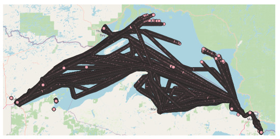
Figure 1. Routes in the selected area with different historical ways. The actual vessel location is at the center.

The GetAIS data process consists of two stages: (a) statistic analysis; and (b) data adjustment. Figure 2 shows several data that exist for our specific target route.

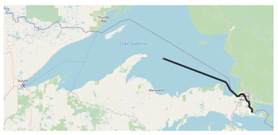
Figure 2. The actual route for a specific target-destination is marked with X.

An analysis of each route’s behavior was undertaken using this method to select the correct data. One drawback is the number of samples that a vessel can record on a whole journey. To understand what is happening in this process, we can describe the statistical analysis identifying central tendency and dispersion measures. Our method uses the Freedman–Diaconis rule to obtain a minimal difference between the area under the empirical probability distribution and the area under the theoretical probability distribution. It will help the method to know the behavior of data, so we can see a gap that can significantly differentiate the routes. The second step is to find visual differences among each route using a histogram and Kernel Density Estimation (KDE). If the KDE or the histogram follows a similar pattern for each route, the data behave similarly. However, that does not occur in real environments.

4.2. Data Adjustment

The graph of the histogram with its probability density curve is in two perspectives. The first uses the calculation of bins through the square root of the amount of data. The second is by using the Freedman–Diaconis rule, as shown in Figure 3 and Figure 4. The last graph is a quantile–quantile one to verify the non-normality of the distribution. Figure 3 and Figure 4 show the sample’s behavior around its histogram and its KDE.

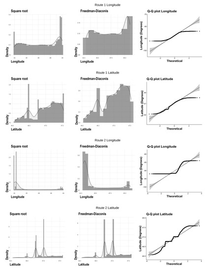
Figure 3. The Kernel Density Estimation (KDE) and histograms for each sample route (one and two) to visualize the differences. Freedman–Diaconis rule was used to calculate bins.

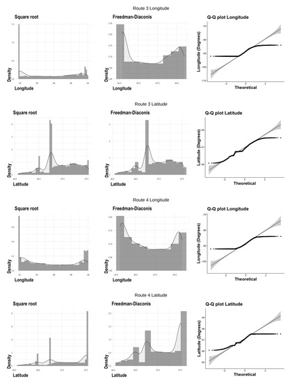
Figure 4. Route 3 and 4 Kernel Density Estimation (KDE) and histograms for each sample route to visualize the differences. Freedman–Diaconis rule is used as a complement of Figure 3.

Some route data change in latitude or longitude, depending on the destination, starting point, or route. The rest of the data are very similar in latitude and longitude. The data are different in the number of observations, or they have small deviations in the routes. At the same time, the historical data contain complete routes. The previous cases (the feature) affect the search and selection of statistical values that serve as discriminant properties to select the appropriate routes that are the basis for predicting and estimating routes.

The first step is to cut the data between the origin and the last actual position values for each route to adjust the sample route to the objective route.

In the target route, the method approximates all AIS data’s statistical behavior to our target and discards those routes with different behavior because some statistical values can perform as outliers, as shown in Figure 5. The data in the red section are discarded. This step helps approximate the historical data to the current route in statistical terms. Some routes have a different direction, and similar cases help to perform the selection of routes in the next step.

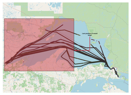
Figure 5. The data in the red section are discarded.

Once the data have been filtered, the method computes the statistical values of each route. All sets of the route with a behavior similar to the target route will maintain a similar statistical behavior despite the lack of information and regardless of the number of observations. This stability is what allows the method to select the most appropriate datasets. It is possible to find statistical values that have a higher weight for classification to detect the best routes that statistically match our route with the Chi-squared selection method. In this case, the method wants to find values with minor and significant statistical differences. The statistics with less dispersion and those with much more dispersion are kept, as shown in Table 1.

Table 1. All statistic values are computed for latitude and longitude, and Route 25 is our route-target.

Routes	Lat Mean	Lat SD	LAT Median	Lat Trimmed	Lat Mad	Lat_Range Range	Lat Skew	Lat Kurtosis	Lat SE	Lon Mean	Lon SD	Lon Median	Lon Trimmed	Lon MAD	Lon Range	Lon Skew	Lon Kurtosis	Lon SE
Route 1	46.7452	0.3696	46.7206	46.743	0.4275	1.327	0.1046	−1.2337	0.0129	−85.1877	0.9905	−84.8746	−85.1019	1.0152	3.2322	−0.5702	−1.0605	0.0344
Route 2	46.749	0.381.043	46.7056	46.7455	0.4358	1.3547	0.1278	−1.2377	0.0124	−85.1737	0.9745	−84.8458	−85.083	0.9356	3.2322	−0.6222	−0.9958	0.0318
Route 3	46.5089	0.0065	46.5124	46.5094	0.0045	0.0261	−0.4288	−1.3778	1 × 10${}^{-4}$	−84.3757	0.0169	−84.3752	−84.3761	0.0046	0.0923	0.1608	0.505	3 × 10${}^{-4}$
Route 4	46.4435	0.1133	46.5032	46.472	0	0.4378	−1.8631	2.2455	0.0034	−84.281.04	0.0884	−84.327	−84.3008	0	0.3288	1.8142	2.0484	0.0026
Route 5	46.81.04	0.3481	46.8522	46.8065	0.4748	1.3192	−0.181.04	−1.1227	0.01	−85.3	0.9396	−85.1586	−85.2475	1.2006	3.2307	−0.347	−1.1476	0.0271
Route 6	46.4254	0.1256	46.5032	46.4515	0	0.4374	−1.3948	0.538	0.0026	−84.2643	0.0986	−84.327	−84.2837	0	0.3308	1.3205	0.3028	0.0021
Route 7	46.4837	0.0687	46.5019	46.5019	1 × 10${}^{-4}$	0.4375	−4.1181.0	16.6474	7 × 10${}^{-4}$	−84.3801	0.0729	−84.4039	−84.4015	6 × 10${}^{-4}$	0.4035	3.4549	11.5551	7 × 10${}^{-4}$
Route 8	46.8939	0.481	46.8786	46.8844	0.5943	1.6987	0.1644	−1.2434	0.0158	−85.2611	0.9821	−85.019	−85.1914	1.1128	3.2296	−0.4605	−1.1327	0.0322
Route 9	46.7512	0.4232	46.5945	46.7296	0.4633	1.8348	0.461	−0.781	0.011	−84.981	0.8673	−84.73	−84.86	0.7228	3.2326	−1.0074	−0.0512	0.0225
Route 10	46.778	0.406	46.814	46.7739	0.506	1.4311	0.0993	−1.3	0.0138	−85.2306	1.0034	−84.9672	−85.1504	1.1148	3.2241	−0.4968	−1.181.0433	0.0342
Route 11	46.9246	0.5221	46.8466	46.9244	0.6756	1.6368	0.0926	−1.6175	0.0159	−85.1424	0.9692	−84.881.04	−85.0452	0.9362	3.2351	−0.6855	−0.8772	0.0296
Route 12	46.7635	0.4111	46.5712	46.747	0.432	1.5004	0.3806	−1.1157	0.0123	−85.1127	0.9484	−84.6995	−85.0081	0.7191	3.2364	−0.7724	−0.781.04	0.0285
Route 13	46.4907	0.0569	46.5041	46.5041	0	0.4487	−5.0681.04	26.4159	4 × 10${}^{-4}$	−84.317	0.0461	−84.3269	−84.3269	0	0.3994	4.5031	22.2307	3 × 10${}^{-4}$
Route 15	46.6236	0.2495	46.6185	46.6358	0.2827	0.9644	−0.3162	−0.9331	0.0083	−85.1146	0.9591	−84.7612	−85.0126	0.8102	3.2341	−0.7423	−0.8197	0.0318
Route 16	47.2569	0.0731	47.2576	47.2571	0.0937	0.2516	−0.0208	−1.2184	0.0055	−86.7552	0.2824	−86.7573	−86.756	0.3608	0.9716	0.0199	−1.2192	0.0212
Route 17	46.5689	0.1847	46.5801	46.5864	0.1882	0.7522	−0.6377	−0.219	0.0058	−85.257	1.0155	−84.9607	−85.1848	1.1244	3.2318	−0.4296	−1.265	0.0318
Route 18	46.5039	0	46.5039	46.5039	0	6 × 10${}^{-4}$	0.3426	2.1018	0	−84.327	0	−84.327	−84.327	0	4 × 10${}^{-4}$	−0.6251	1.6465	0
Route 21	46.7151	0.3522	46.5295	46.7047	0.3831	1.3261	0.3276	−1.0741	0.0116	−85.0743	0.9629	−84.6554	−84.9644	0.7026	3.2318	−0.81.043	−0.7722	0.0316
Route 22	46.8493	0.5226	46.7481	46.8032	0.4595	2.1414	0.8019	0.1072	0.0155	−84.9308	0.7366	−84.8472	−84.8397	0.7367	3.2328	−1.2027	1.4906	0.0218
Route 23	46.7484	0.3686	46.7232	46.7462	0.4231	1.3252	0.1032	−1.2429	0.0129	−85.1956	0.9924	−84.8829	−85.1105	1.0158	3.232	−0.5567	−1.0834	0.0346
Route 24	46.5917	0.1751	46.6034	46.6097	0.1627	0.7872	−0.8153	0.4608	0.0048	−85.0913	0.8171	−84.9781	−84.985	0.7554	3.2322	−1.0473	0.3076	0.0225
Route 25	46.7896	0.3441	46.8456	46.81.04	0.4713	1.2992	−0.1852	−1.1293	0.01	−85.2761	0.9208	−85.1329	−85.2259	1.1676	3.1519	−0.3408	−1.163	0.0267

The statistical metrics calculated for the vessel position’s target routes (longitude and latitude) are as follows:

The mean is obtained from the tracking of each route. A central descriptive value is obtained from the distribution of the routes. The main disadvantage is the mean is susceptible to outliers’ influence, a property that the method can use as a discriminant feature.

Standard deviation measures the dispersion around the mean. It is highly influenced by the mean and allows the identification of outliers. This property is used to select the closest routes to the route that will generate the prediction.

The median is selected because outliers do not influence it. In addition, it provides an approximate location of the center point to the distribution when it is not normal to the target path distribution.

The trimmed mean is less sensitive to outliers. It allows discarding them and uses the distribution data to get closer to the target route.

MAD is less sensitive to outliers. It is an important variable to relate the routes that are statistically similar to the target route.

The range is susceptible to outliers. This property allows discriminating those routes that have large deviations outside the target route.

Skew identifies the degree of distortion of the distribution and is a characteristic most used as a discriminant.

Kurtosis is a statistical measure to discriminate by focusing on the tails of the distribution. It identifies outliers and routes that have deviations.

Standard Error of Mean (SE) rates the uncertainty in estimating the mean of the target route data compared to the other historical routes.

The selection operation is not strict because the routes can have a statistical similarity from the point of origin to the set point. The consequence is selecting routes with different weights for training and influencing the precision of the method.

Of the previous variables, MAD is one of the most stable variables depending on its nature, regardless of the number of observations, as shown in Figure 6.

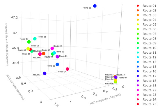
Figure 6. A three-dimensional perspective of three features of the routes, two of which are MAD.

Therefore, it is the variable that determines the selection of significant routes. The range is quite sensitive to the characteristics of the dataset because it is altered significantly by the existence of outliers.

As mentioned above, Table 1 shows the statistical values of each route as features. The data have a marked difference in most of the statistical values, specifically those related to latitude. The method applies the cluster technique to those statistical values to help us choose the best prediction routes. The cluster is on densities. The dense region of objects contains a target path and similar paths. The low-density section is those routes with a statistical difference.

5. Experiments

This section uses input data analysis and the selection of those statistical values that represent the best way for each route. A clustering technique was used and the data were selected to predict the route.

The process of finding and predicting the position of the vessel movements consists of three stages: (a) route selection by clustering; (b) using an artificial neural network; and (c) using multivariate imputation by chained equations.

5.1. Route Selection by Clustering

Density-Based Spatial Clustering of Applications with Noise (DBSCAN) [29] was applied to discover and select the best data. DBSCAN was proposed by Albert Ester and can identify clusters and outliers. A clear difference before the application of DBSCAN is found in the sample.

The first step is to cut the 146 data (for each route) between the origin and the last actual position values (147 longitudes and latitudes approximately) of the target route to adjust the sample routes to the objective route.

The route selection helps approximate all 148 AIS data’s statistical behavior to the target and discards those routes with different behavior. Some of the 149 statistical values are outliers, as shown in Figure 7.

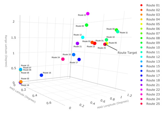
Figure 7. The actual and predicted routes.

The configuration parameters of DBSCAN are related to the minimum distance found at each point, and the minimum elements of clusters are defined by 3. The method applies DBSCAN to see several groups within its routes, as shown in Figure 8.

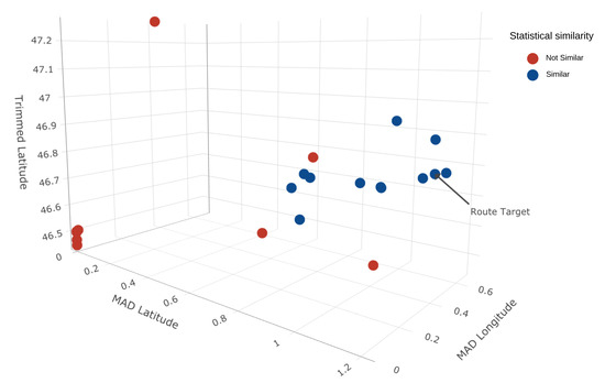
Figure 8. Cluster discovered using DBSCAN. Those routes in the group (tagged as Similar) have a similarity in statistical properties and help predict and estimate the route-target.

After applying DBSCAN, the method discards all routes that do not resemble the route to predict. For better results, it is necessary to have enough data to get an accurate approximation of its best statistical values to achieve the classification’s performance according to the theorem of limit central [30]. The algorithm chooses the information that justifies the use of specific routes that share similarities with the target.

The method’s comparison is with the methodological approach for extraction of the characteristics of biological signals [31], which uses the histogram class marks to make the selection of characteristics using the behavior of the distribution of biological signals.

The classmark allows a representative point of each histogram interval to be obtained and then a frequency polygon to be created. A frequency polygon is built with a dynamic prototype and biological signals to get a graphic form to represent the original data.

Table 2 shows the comparative results of route selection for each method, which are almost all similar. The differences are in the features. PreMovEst can use a small number of features to select routes. In contrast, the methodological approach for the extraction of biological signals’ characteristics needs all features, multiplying the number of latitude and longitude features.

Table 2. The results of route selection for all methods are similar.

Clustering after Using PreMovTest	Clustering after Using Granados-Ruiz 2019	Route
1	1	Route 1
1	1	Route 2
0	0	Route 3
0	0	Route 4
1	1	Route 5
0	0	Route 6
0	0	Route 7
1	0	Route 8
1	0	Route 9
1	1	Route 10
1	0	Route 11
1	0	Route 12
0	0	Route 13
1	0	Route 15
0	0	Route 16
0	0	Route 17
0	0	Route 18
1	1	Route 21
0	0	Route 22
1	1	Route 23
0	0	Route 24
1	1	Route 25

For prediction and route estimation, the selection of all routes that resemble the current route was made. First, an Artificial Recurrent Neural Network (ARNN) with Long Short-Term Memory (LSTM) was used with historical data as continual input streams. As the second technique, multivariate imputation by chained equations used a statistical method for handling missing data.

The sample contains almost 158,274 records for training in the case of an Artificial Neural Network (ANN). For the application of MICE, all records were used, including records of the actual vessel target.

In addition, for both techniques, only longitude and latitude were used to save computational power.

5.2. Using an Artificial Neural Network

The type of ANN used before was an ARNN with a Long Short-Term Memory layer using Keras high-level framework [32].

First, some variables were defined: the network is made up of three layers, with 64 neurons in the input layer, 32 in the intermediate layer, and two neurons for the output layer, as shown in Figure 9.

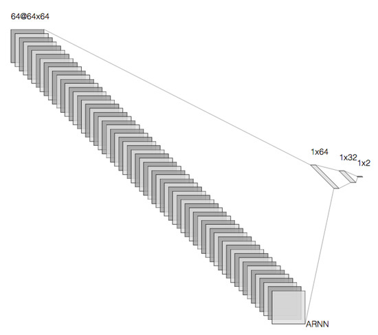
Figure 9. The neural network architecture.

The method learns through an adaptive prediction model and automatically determines when the next position on a vessel’s route occurs. A knowledge base was generated with all routes of the target vessel to achieve this goal. The first part of the data was used to create a model to predict the routes. Besides, the filtered historical data were used to train, validate, and test the neural network model to predict the current route.

5.3. Using Multivariate Imputation by Chained Equations

MICE is widely used to search for missing dataset values to get the best cases about data behavior [33].

For the full application of this technique, it was necessary to carry out a stratified sampling. The algorithm obtains a representative matrix of the data to get the most important information that contributes to generating the estimation route.

6. Results

The purpose was to show that, after obtaining the journey knowledge base, our method helps in the selection of the routes based on the statistical behavior of each one. ANN achieved the prediction of an interval of time and the estimation of the route using the MICE Algorithm. The PreMovEst method obtained the following results: Table 3 shows a contrast between the actual data of an interval of time and the ANN’s vessel movement predictions.

Table 3. Real data versus the predicted path segment. The predicted latitude has better accuracy than the predicted longitude.

Original Latitude	Predicted Latitude	Original Longitude	Predicted Longitude
47.36767	47.88345	−87.16083	−86.99632
47.36887	47.99324	−87.16616	−86.54012
47.37018	48.01275	−87.17136	−86.62076
47.3715	48.02375	−87.17667	−86.56543
47.37282	48.11034	−87.18205	−87.18984
47.37396	48.11498	−87.1872	−87.22098
47.37532	48.12876	−87.19258	−87.35465
47.37667	48.12076	−87.19767	−87.65703
47.378	48.13776	−87.203	−87.98583
47.381.04333	48.22021	−87.20817	−87.99232

Table 3 presents ten positions of Route 25 of Segments 15 and 16. The results show an accuracy of 80.5% in the prediction. However, if the method does not have enough information about the route to be estimated or it is too short, it loses precision. That is why we combine the two processes: prediction using neural networks and route estimation with MICE. Besides, where there is not enough information, it is necessary to obtain more historical data, which increases the processing time that depends on the amount of AIS.

The amount of information used in the second example was more than in the first one. That allowed the accuracy to be better, at 84%. The historical AIS data samples are similar from the block to be estimated, out of 10 predictions. The absolute mean difference for latitude is 0.0015655 degrees, while the absolute mean difference for longitude is 0.00211949 degrees, as shown in Table 4.

Table 4. Real data contrasted with the previously predicted path segment on the second sample.

Original Latitude	Predicted Latitude	Original Longitude	Predicted Longitude
47.36767	47.88345	−87.16083	−86.99632
47.36887	47.99324	−87.16616	−86.54012
47.37018	48.01275	−87.17136	−86.62076
47.3715	48.02375	−87.17667	−86.56543
47.37282	48.11034	−87.18205	−87.18984
47.37396	48.11498	−87.1872	−87.22098
47.37532	48.12876	−87.19258	−87.35465
47.37667	48.12076	−87.19767	−87.65703
47.378	48.13776	−87.203	−87.98583
47.381.04333	48.22021	−87.20817	−87.99232

Concerning the MICE technique’s application, as shown in Figure 10, the prediction generates the route approximation with 76.15% accuracy, using a small sample of routes. Finally, the prediction obtained an accuracy of 81.043%. However, it allows for approximating the results with the ten routes as the sample.

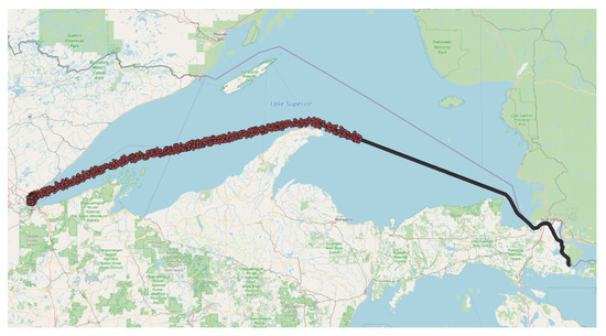
Figure 10. The route prediction results with MICE.

The PreMovEst method shows that the prediction is almost the same as the real one after selecting the best routes.

The best routes (series of positions) have a similarity in statistical properties after the clustering process.

The routes’ selection through their statistical data in the clustering allows discriminating those routes whose navigation course differs from the current route predicted. That is why they work as outliers, which is evident when clustering carried out, as they remain outside the cluster to which the route to be estimated belongs.

Figure 10 compares the PreMovEst method to the Zissis method that considers a cloud infrastructure to support marine traffic. Furthermore, their system stores the trained vessel and recalls it 24 h as input for the following predictions. Our method uses data in real-time and is capable of running on a computer with GPU. Computing power is demanded, depending on the application. Our method contributes to the search for processes that allow computational savings. It is understood that a dataset can be better known if it has the largest number of characteristics.

In the second example (see Figure 11), the method used more historical AIS data samples, i.e., 28% more than the first example. There is more information to predict the next movements of the route. In addition, the complete route was estimated. In this example, the historical samples are quite similar to the target route. It is also favorable because the route block to be estimated is smaller than in the previous example.

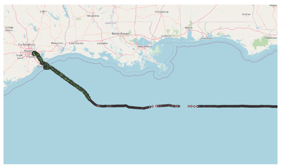
Figure 11. The route prediction results with MICE.

A segment of the original route with no information was observed. It occurred for technical reasons and was compensated by the historical information extracted in the selection process; however, our objective is not to recover missing data, which can lead to missing historical information. Thus, the neural network’s prediction process would be more uncertain when there are missing data in the segment to be estimated.

7. Conclusions

The present proposal, called Method for Select Best AIS Data in Prediction Vessel Movements and Route Estimation (PreMovEst), is related to obtaining reports on vessels’ status that allows for accurate and real-time monitoring.

It applies to all vessels navigating within a designated maritime area and predicting future positions of a vessel based on positions already traveled within the designated maritime area. The information is shown to the user through general and specific vessel status reports.

The PreMovEst method was tested using a small dataset. However, the correct selection of data for analysis and prediction in maritime routes is essential before applying the method.

The PreMovEst method uses a filter for the routes whose behavior are similar to obtain the best routes collection through a Chi-squared selection process. The execution time was reduced from 16 to 11 min on average. The experiments were run on a Core i7 processor with 16 GB of RAM.

The results show a prediction accuracy of 80.5–84%. The amount of information used in the second example was more than the first example, which allowed the accuracy to be better, at 84%. The historical AIS data samples are similar to the block to be estimated, out of 10 predictions. The absolute mean difference for latitude is 0.0015655 degrees, while the absolute mean difference for longitude is 0.00211949 degrees.

The results concern the assets of the vessels that move in the seas, especially in economic terms. The paper shows the PreMovEst method’s application and testing of its accuracy using ARNN and MICE techniques. Everyday, vessels move billions of items across the oceans from one country to another, a drawback of which is handling all of this information. The process of selecting data to train the neural network is a function of the number of trips made by the vessel from the port of departure to the arrival port.

One of the challenges to be undertaken is to obtain better accuracy while reducing the execution time.

Future work will be to accelerate the prediction model with Graphical Process Units (GPU). This requires image processing, which implies supercomputers to process such data, limiting its effectiveness for real-time monitoring of vessels navigating within a designated maritime area and increasing the amount of processed information.

References

- ANAVE. Merchant Marine and Maritime Transport 2017/2018. 2018. Available online: https://unctad.org/system/files/official-document/rmt2018_en.pdf (accessed on 9 December 2020).
- Deng, F.; Guo, S.; Deng, Y.; Chu, H.; Zhu, Q.; Sun, F. Vessel track information mining using AIS data. In Proceedings of the 2014 International Conference on Multisensor Fusion and Information Integration for Intelligent Systems (MFI), Beijing, China, 28–29 September 2014; pp. 1–6. [Google Scholar] [CrossRef]
- Alessandrini, A.; Alvarez, M.; Greidanus, H.; Gammieri, V.; Arguedas, V.F.; Mazzarella, F.; Santamaria, C.; Stasolla, M.; Tarchi, D.; Vespe, M. Mining Vessel Tracking Data for Maritime Domain Applications. In Proceedings of the IEEE International Conference on Data Mining Workshops (ICDM 2016), Barcelona, Spain, 12–15 December 2016; pp. 361–367. [Google Scholar] [CrossRef]
- Pallotta, G.; Vespe, M.; Bryan, K. Vessel pattern knowledge discovery from AIS data: A framework for anomaly detection and route prediction. Entropy 2013, 15, 2218–2245. [Google Scholar] [CrossRef]
- Perera, L.P.; Oliveira, P.; Guedes Soares, C. Maritime Traffic Monitoring Based on Vessel Detection, Tracking, State Estimation, and Trajectory Prediction. IEEE Trans. Intell. Transp. Syst. 2012. [Google Scholar] [CrossRef]
- Zissis, D.; Xidias, E.K.; Lekkas, D. Real-time vessel behavior prediction. Evol. Syst. 2016, 7, 29–40. [Google Scholar] [CrossRef]
- Mazzarella, F.; Arguedas, V.F.; Vespe, M. Knowledge-based vessel position prediction using historical AIS data. In Proceedings of the 2015 Workshop on Sensor Data Fusion: Trends, Solutions, Applications (SDF), Bonn, Germany, 6–8 October 2015. [Google Scholar] [CrossRef]
- Hexeberg, S.; Flåten, A.L.; Eriksen, B.H.; Brekke, E.F. AIS-based vessel trajectory prediction. In Proceedings of the 2017 20th International Conference on Information Fusion (Fusion), Xi’an, China, 10–13 July 2017; pp. 1–8. [Google Scholar] [CrossRef]
- Vanneschi, L.; Castelli, M.; Re, A. Prediction of ships’ position by analysing AIS data: An artificial intelligence approach. Int. J. Web Eng. Technol. 2017, 12, 253. [Google Scholar] [CrossRef]
- Zhang, C.; Bin, J.; Wang, W.; Peng, X.; Wang, R.; Halldearn, R.; Liu, Z. AIS data driven general vessel destination prediction: A random forest based approach. Transp. Res. Part C Emerg. Technol. 2020, 118, 102729. [Google Scholar] [CrossRef]
- Liu, J.; Shi, G.Z.K. Vessel Trajectory Prediction Model Based on AIS Sensor Data and Adaptive Chaos Differential Evolution Support Vector Regression (ACDE-SVR). Appl. Sci. 2020, 9, 15. [Google Scholar] [CrossRef]
- Wang, C.; Ren, H.; Li, H. Vessel trajectory prediction based on AIS data and bidirectional GRU. In Proceedings of the 2020 International Conference on Computer Vision, Image and Deep Learning (CVIDL), Nanchang, China, 15–17 May 2020; pp. 260–264. [Google Scholar] [CrossRef]
- Dobrkovic, A.; Iacob, M.; van Hillegersberg, J.; Mes, M.; Glandrup, M. Towards an Approach for Long Term AIS-Based Prediction of Vessel Arrival Times. In Logistics and Supply Chain Innovation: Bridging the Gap between Theory and Practice; Lecture Notes in Logistics; Zijm, H., Klumpp, M., Clausen, U., ten Hompel, M., Eds.; Springer: Berlin, Germany, 2015; pp. 281–294. [Google Scholar] [CrossRef]
- Tu, E.; Zhang, G.; Mao, S.; Rachmawati, L.; Huang, G.B. Modeling Historical AIS Data For Vessel Path Prediction: A Comprehensive Treatment. arXiv 2020, arXiv:2001.01592. [Google Scholar]
- Alizadeh, D.; Alesheikh, A.A.; Sharif, M. Vessel Trajectory Prediction Using Historical Automatic Identification System Data. J. Navig. 2021, 74, 156–174. [Google Scholar] [CrossRef]
- Ramin, A.; Mustaffa, M.; Ahmad, S. Prediction of Marine Traffic Density Using Different Time Series Model From AIS data of Port Klang and Straits of Malacca. Trans. Marit. Sci. 2020, 9, 217–223. [Google Scholar] [CrossRef]
- Young, B.L. Predicting Vessel Trajectories from AIS Data Using R. Master’s Thesis, Naval Postgraduate School, Monterey, CA, USA, 2017. [Google Scholar]
- Filipiak, D.; Stróżyna, M.; Węcel, K.; Abramowicz, W. Big Data for Anomaly Detection in Maritime Surveillance: Spatial AIS Data Analysis for Tankers. Zesz. Nauk. Akad. Mar. Wojennej 2018, 215, 5–28. [Google Scholar] [CrossRef][Green Version]
- Xin, X.; Liu, K.; Yang, X.; Yuan, Z.; Zhang, J. A simulation model for ship navigation in the “Xiazhimen” waterway based on statistical analysis of AIS data. Ocean. Eng. 2019, 180, 279–289. [Google Scholar] [CrossRef]
- Daranda, A.; Dzemyda, G. Navigation Decision Support: Discover of Vessel Traffic Anomaly According to the Historic Marine Data. Int. J. Comput. Commun. Control. 2020, 15. [Google Scholar] [CrossRef]
- Alessandrini, A.; Mazzarella, F.; Vespe, M. Estimated Time of Arrival Using Historical Vessel Tracking Data. IEEE Trans. Intell. Transp. Syst. 2019, 20, 7–15. [Google Scholar] [CrossRef]
- Gao, M.; Shi, G.Y. Ship-handling behavior pattern recognition using AIS sub-trajectory clustering analysis based on the T-SNE and spectral clustering algorithms. Ocean Eng. 2020, 205, 106919. [Google Scholar] [CrossRef]
- Bautista, R.; Barbosa-Santillán, L.; Sánchez-Escobar, J. Statistical Approach in Data Filtering for Prediction Vessel Movements Through Time and Estimation Route Using Historical AIS Data. In Proceedings of the Mexican International Conference on Artificial Intelligence, Xalapa, Mexico, 27 October–2 November 2019; pp. 28–38. [Google Scholar] [CrossRef]
- U.S. Department of Commerce’s National Oceanic and Atmospheric Administration (NOAA) Office for Coastal Management and the U.S. Department of the Interior’s Bureau of Ocean Energy Management (BOEM). MarineCadastre. 2019. Available online: https://marinecadastre.gov/ais/ (accessed on 9 December 2020).
- Williams, R.J.; Zipser, D. A Learning Algorithm for Continually Running Fully Recurrent Neural Networks. Neural Comput. 1989, 1, 270–280. [Google Scholar] [CrossRef]
- Hochreiter, S.; Urgen Schmidhuber, J. LONG SHORT-TERM MEMORY. Neural Comput. 1997, 9, 1735–1780. [Google Scholar] [CrossRef] [PubMed]
- Gers, F.A.; Schmidhuber, J.; Cummins, F. Learning to forget: Continual prediction with LSTM. Neural Comput. 2000. [Google Scholar] [CrossRef] [PubMed]
- White, I.R.; Royston, P.; Wood, A.M. Multiple imputation using chained equations: Issues and guidance for practice. Stat. Med. 2011, 30, 377–399. [Google Scholar] [CrossRef] [PubMed]
- Ester, M.; Kriegel, H.P.; Sander, J.; Xu, X. A Density-based Algorithm for Discovering Clusters a Density-based Algorithm for Discovering Clusters in Large Spatial Databases with Noise. In Proceedings of the Second International Conference on Knowledge Discovery and Data Mining (KDD’96), Portland, OR, USA, 2–4 August 1996; pp. 226–231. [Google Scholar]
- Peck, R.; Devore, J.L. Statistics: The Exploration & Analysis of Data; Cengage Learning: Boston, MA, USA, 2011. [Google Scholar]
- Granados-Ruiz, J.; Hernandez, D.A.G.; Ramírez, C.L.; Zamudio, V.; Pérez-Mata, P. Methodological approach for extraction of characteristics of biological signals. Compusoft 2019, 8. [Google Scholar]
- Chollet, F. Keras Documentation. 2015. Available online: https://github.com/fchollet/keras (accessed on 9 December 2020).
- Azur, M.J.; Stuart, E.A.; Frangakis, C.; Leaf, P.J. Multiple imputation by chained equations: What is it and how does it work? Int. J. Methods Psychiatr. Res. 2011. [Google Scholar] [CrossRef] [PubMed]
Publisher’s Note: MDPI stays neutral with regard to jurisdictional claims in published maps and institutional affiliations. |
© 2021 by the authors. Licensee MDPI, Basel, Switzerland. This article is an open access article distributed under the terms and conditions of the Creative Commons Attribution (CC BY) license (http://creativecommons.org/licenses/by/4.0/).