An Algorithm for Rescheduling of Trains under Planned Track Closures

Abstract

This work considered a joint problem of train rescheduling and closure planning. The derivation of a new train run schedule and the determination of a closure plan not only must guarantee the satisfaction of all the given constraints but also must optimize the number of accepted closures, the number of approved train runs, and the total time shift between the resultant and the original schedule. Presented is a novel nonlinear mixed integer optimization problem which is valid for a broad class of railway networks. A multi-level hierarchical heuristic algorithm is introduced due to the NP-hardness of the considered optimization problem. The algorithm is able, on an iterative basis, to jointly select closures and train runs, along with the derivation of a train schedule. Results obtained by the algorithm, launched for the conducted experiments, confirm its ability to provide acceptable and feasible solutions in a reasonable amount of time.

1. Introduction and Contributions

1.1. Introduction

Scheduling of trains resulting in customer-friendly timetables is a crucial management task in railway transportation. The determination of a schedule of trains is a complex and a challenging thing in itself, even if solved in the presence of full, crisp, and stable information, e.g., References [1,2,3,4]. Unfortunately, such information is unavailable in real-world conditions when different disruptions can occur. Despite a variety of reasons for the disruptions, all of them result in derogation from timetables and delayed arrivals at destinations for railway customers. The outages can be unplanned, e.g., due to infrastructure and facility breakdowns, the acts of God or planned, e.g., connected with the preventive maintenance of infrastructure. Considerations in the paper are focused on the latter case when planned closures of tracks (also named possessions) are taken into account. From now on, a closure is understood as a period when a part of a rail network, i.e., a defined collection of rail tracks, is not available for trains. A case with a given set of closures is only investigated in the paper. Each closure affects an ongoing timetable. A collection of closures can bring about the modification of trains’ arrival and departure times at stations (and other points on of the railway network—further called stations—where merging/division of tracks can take place or where trains can overtake one another or stop) or even the cancellation of some trains. The change of an ongoing timetable for trains is called the train rescheduling, which is obligatory due to the necessity to manage a given set of closures. Depending on a size of the set of closures, as well as durations of closures and their time and place relationships, the acceptance of all closures may not be possible. So, the proper closure planning is necessary as it allows for a trade-off between the possibly highest number of accepted closures and the as small as possible deterioration of the original timetable for trains. Such planning and the rescheduling of trains are two important tasks faced by railway transportation operators.

1.2. Contributions and Structure of the Paper

Unlike most of the existing works, we consider train rescheduling and closure planning as a joint optimization task modeled as the nonlinear mixed integer optimization problem. Due to its high complexity, we propose a heuristic algorithm which is based on a decomposition of the problem into smaller sub-problems.

Current considerations refer to Reference [5] and extend it, taking into account the possibility of train rerouting. In our approach, a new route may be determined as any track sequence along a given path (sequence of stations), and it may also include the substitute transportation for some of them. Moreover, the proposed method of rerouting can be further enhanced, as it was done in Reference [6], where the authors analyze a rerouting mechanism that permits changes in the order and the number of tracks visited by a train.

The novelty of our contribution is three-fold:

• First, we formulate a novel joint train rescheduling and closure planning as the nonlinear mixed integer optimization problem valid for a wide class of railway networks with the possibility of rerouting and substitutive transport launching. Moreover, our model allows to control each event (e.g., each train runs conflict) independently, in contrast to the methods applying aggregated approach e.g., as the one presented in Reference [7]. The proposed model and resulting algorithms enable solving investigated decision-making problems for general railway networks, but they have been developed taking also into account the specificity of such networks in Poland.
• Second, due to the high complexity of the formulated initial problem, we propose a multi-level heuristic solution algorithm based on the decomposition allowing the solution of smaller-size sub-problems. The choice of the heuristic algorithm suitable for real-world applications is justified by the NP-hardness of the problem. The proposed formulation of the optimization problem allows for the rationale of this property.
• Third, we confirm the usefulness of the algorithm via the extensive simulation experiments using both randomly generated data but also data originated from the real-world railway network comprising almost 150 stations and 100 trains. The remainder of this paper is organized as follows. Closure planning practices in Poland are outlined in Section 3, and it follows a brief review of related work given in Section 2. The next section presents the model of the considered joint problem of train rescheduling and track closure planning which is based on the graph-matrix representation of a railway network, a train runs timetable, and track closures. Section 5 is devoted to the detailed description of proposed heuristic solution algorithm. The results of experimental evaluation of the algorithm, both for a single track and, first of all, for a real-world case, are given in Section 6. A real-world railway network consisting of up to 95 train runs and 149 train stations serves for the evaluation of the algorithm’s quality with respect to different algorithm’s, as well as problem’s, parameters. Final remarks complete the paper.

2. Related Work

The problem of train rescheduling under planned closures consists of two partial problems which can be treated separately, and those separate approaches are included in the literature survey. From the standpoint of this paper, however, simultaneous consideration of both partial problems is of greater importance, and, for that reason, the literature review focuses on the joint problem. Finally, since the paper targets the railway network in Poland, a portion of the review is dedicated to local models and methods.

Since the volume of papers dedicated to scheduling of trains and closure planning in railway transportation is considerable, only selected works can be included in a non-dedicated review paper. For additional survey of recent literature, we refer the reader to References [8,9].

2.1. Train Rescheduling

The train rescheduling task is a problem quite widely discussed in the literature. It is understood, in the most cases, as the response to a single unforeseen event that prevents the further realization of the transportation plan by the original timetable. As detailed in Reference [10], the problem of rescheduling can be handled as different (re-)scheduling paradigms: offline, done to establish a primary schedule; and online, done mainly to reestablish a schedule that is no longer acceptable (feasible). The main difference, from the standpoint of difficulty of solving is that the former approach can be performed over a significantly longer period of time, while the latter needs to be done quickly, so as not to allow operations on an invalid schedule. The latter approach can, and likely will, lead to such problem formulations and solution algorithms which, in general case, forgo optimality and focus on providing heuristic, sub-optimal solutions instead. It is this approach that we focus on in this paper, although the results can also be applied to formulate a primary schedule. Online approaches can be further divided into static (open-loop) and dynamic (closed-loop), where, in the dynamic cases, not all of the information is readily available during the decision-making process. As new information about decision execution becomes available, it is fed back to the rescheduling algorithm and (possibly) results in new solutions. Finally, prediction of future states of the system is taken into consideration in proactive approaches, as opposed to reactive ones.

The mixed integer programming (MIP) model is proposed in Reference [11] for the train rescheduling problem when a train’s initial delays are given, and the minimization of the total delay of all passengers is required. However, specific requirements resulting from the state of railway infrastructure are not taken into account in this work. It is assumed that every route can hold any number of train runs in the same period. The extension of this problem is presented in Reference [12], where the limited number of train runs traveling between two stations at a given time is considered. The problem is formulated using integer linear programming approach and solved using the branch and bound method. Real-world data provided by Deutsche Railways have made it possible to test this approach successfully. A similar model and solution algorithm based on the Lagrange relaxation is proposed in Reference [13]. As a consequence, the problem is decomposed into a sequence of simple optimization tasks each corresponding to one train run. Another integer programming model presented in Reference [14] considers the assumption that, between any two stations, there is no more than one track, which may be occupied by no more than one train run at the same time. However, the authors do not propose any solution to the formulated problem due to its computational complexity. The authors in Reference [15] assume that there are always two tracks between two connected stations, and each of them may be occupied by no more than one train run at the same time. In this case, the genetic algorithm is applied to solve the train rescheduling problem. The discrete dynamic optimization model for train rescheduling problem is given in Reference [16]. The main goal in this case is to maximize punctuality and station satisfaction degree. However, authors also limit their consideration to the single-track railway and, even for this simple scenario, apply the heuristic approach.

More complex models of railway network infrastructure are presented in Reference [17], where it is taken into account that tracks are composed of blocks, and there may be any number of tracks between stations. The optimization model, formulated as a mixed linear programming task, consists of the minimization of two objectives: the total cost of delays and the total time of delays. The CPLEX software was applied to solve the problem. A similar approach is proposed in Reference [18]. Assumptions about railway infrastructure are also adopted in Reference [19], where two methods are proposed. The first one is based on MIP, while the second one uses Constraint Programming. Similarly, the timetable rescheduling, rolling stock rescheduling, and crew (train drivers) rescheduling problems are formulated in Reference [20] using integer programming models. In the mentioned paper, the timetable rescheduling problem is treated as the job shop scheduling, the rolling stock rescheduling problem is presented using the multi-commodity flow in a graph model, and the crew rescheduling problem is seen as the extended set covering. Further research has been done in providing an approach of exchanging blocks of routes with permitted alternative blocks through the means of alternative graph formulations [21,22]. One can also find adaptations of graph methods [23], such as time-space models [24].

As models considering the accurate description of railway infrastructure require too many computational resources to solve problems exactly in an acceptable amount of time, some more time efficient methods and heuristics are often applied. For example, in Reference [25], the authors propose a new approach based on the Statistical Analysis of Propagation of Incidents method, and, in Reference [26], a two-stage procedure is proposed. The first stage rests on the Simulated Annealing and the Tabu Search metaheuristics, whereas the second stage solves a simple integer programming problem. An approach based on MIP that incorporates a possibility of rerouting trains to enable minimizing the number of canceled and delayed trains, while adhering to infrastructure and rolling stock capacity constraints, is presented in Reference [27]. A proposition to apply MIP model to increase a robustness of the timetables is described by authors of Reference [28]. Considerations of the rescheduling problem on a single track unidirectional rail line that adheres to a cyclic schedule are included in Reference [29], where it is assumed that two types of trains (express and local) are dispatched from the origin in an alternating manner. The application of mixed integer programming to minimize combined length of shipping cycle and total dwell time of local trains at all stations is presented. In Reference [30], the authors consider the problem of adjusting the timetable in a case of partial or complete deadlocks. The integer programming formulation is given with the maximization of a service level.

A recent macroscopic approach was presented in Reference [31], where boundary passenger runs within an urban network were tackled. The authors propose a mixed integer programming approach with the use of a space-time network. This is solved for large instances with the use of decomposition. In Reference [32], the authors turn to microscopic modeling of the railway network and consider a problem of rescheduling in dense railway systems which are subject to disturbances. A multi-objective optimization problem is solved heuristically. In Reference [33], a problem of deadhead routing in an urban transit line was tackled. The authors formulate it as an MIP problem which is solved with the use of a CPLEX solver with an embedded branch-and-cut algorithms.

2.2. Closure Planning

The papers on the closure planning and, more generally, maintenance scheduling problems or even the maintenance management usually take into account the need of introducing to train timetables a delay as little as possible. Considerations in Reference [34] are focused on the local impact of maintenance on the railway infrastructure. Moreover, the limitation to single routes is taken into account in References [35,36,37,38]. In these papers, the problem of timetable planning is not solved. Instead, the scheduling of maintenance activities is formulated to minimize their impact on a original schedule. According to the argumentation in Reference [36] that such a problem is NP-hard, the application of some heuristic algorithms is appropriate, e.g., in Reference [38], the authors proposed the ant colony optimization method. In Reference [39], authors formulate the problem of planning maintenance windows, which is a concept incorporated by Swedish railways. This particular idea consists of the inclusion of train-free time slots into the tracks during timetable planning. The time windows for potential track closures and their durations are determined in advance, while the train traffic is described regarding statistical flows instead of a final timetable. More detailed surveys on railway maintenance planning activities may be found in References [40,41].

More recently, in Reference [42], a problem of scheduling maintenances in a large-scale network of trams was considered. The authors formulate an MIP and solve it with the use of neighborhood search-like heuristic approach.

2.3. Joint Approaches

Some important suggestions for the joint consideration of the maintenance activities scheduling and the train run rescheduling are indicated in References [43,44]. It is pointed out there that a single closure of a track indispensable for the completion of a maintenance activity could be treated as a particular type of train, but the idea has not been sufficiently developed. The concept of a system that helps to plan the closure of tracks with the simultaneous consideration of changes in the timetable is presented in Reference [45]. However, the solution is not based on a formal mathematical model, and the authors assume that new schedules are determined by external systems rail carriers. The joint scheduling of maintenance of the infrastructure (track closures) and rescheduling of train runs is also discussed in References [46,47]. In Reference [47], the author addresses the case when train arrival and departure times may be changed, but train runs cannot be canceled. Two analytical approaches are proposed, i.e., MIP (additionally with the bound and price reduction) and Problem Space Search metaheuristic, which was also presented in Reference [46]. This heuristic allows to generate alternative timetables and then to combine obtained solutions into one final timetable. MIP models are also proposed in References [7,48] for the joint closure planning and timetabling problem. This model includes the possibility of changing train routes, as well. However, it is assumed that such train rescheduling may be performed among a finite number of alternatives given in advance.

Unlike in our work, in Reference [48], the authors assumed that all closures are obligatory and in Reference [49], the authors do not consider particular events concerning conflicts between train runs; instead, they apply flow-based approach which is modeled as MIP with implicit link usage variables and cumulative station entry/exit variables. This model is solved with a Gurobi solver in Python and tested on a set of self-generated instances. In Reference [50], a reformulation is made—link usage variables are made explicit, while entry/exit variables are now binary. This model is further extended in Reference [51] to include crew scheduling.

Train scheduling and preventive maintenance are also jointly considered in Reference [52], where the sum of absolute arrival time deviations of real trains at destinations between the identical and actual timetables is minimized. A proactive approach to planning maintenance windows is presented as the authors try to ensure that maintenance work is already included in the schedule. The problem is formulated as an MIP and solved with the use of Lagrange relaxation. Another MIP approach presented in Reference [53] is aimed at incorporating new closures in a way that disturbs the original schedule the least. This approach is tested on date from a cut-out of the Netherlands railway system. An MIP approach tested on the French railway network can be found in Reference [54].

The authors of Reference [8] develop a microscopic approach, where timetabling and maintenance scheduling is formulated as a mixed integer programming problem. To alleviate computational difficulties of finding an exact solution, an iterative algorithm based on decomposition is proposed. It is shown that it results in near-optimal solutions for the tested cases. For Reference [55], an MIP formulation was applied to high-speed networks, where, in order to alleviated maintenance-induced problems, switches to normal-speed network were employed. Finally, in Reference [9], the authors use a dynamic constraint-generation technique coupled with Lagrangian relaxation for a double-track network with transmittable maintenances. The method was proven effective on a small section of a Chinese railway system.

Mixing the microscopic and the macroscopic approaches leads to intermediate, so-called mesoscopic models. As an example, in Reference [56], the authors consider a two-stage algorithm as a means of problem decomposition which speeds-up the algorithm execution time. The algorithm is tested on a network of 66 stations in case of a single, full blockade of a selected connection. This approach is further explored in Reference [57], where online, closed-loop rescheduling is done with the use of model model predictive control.

Further integration of traffic control and train operation is considered in Reference [58], where train speeds are considered. The authors formulate a nonlinear integer programming problem which they then simplify by approximating the nonlinearities with piecewise linear functions. To solve the many formulated sub-problems, the authors use a solver, a genetic algorithm and a custom procedure. The method is tested on a railway network of 40 nodes. In Reference [59], the authors consider two control loops: inner, which is responsible for managing immediate train operation and outer, where traffic control is done. The authors focus on Automated Train Operation subsystem of the Automatic Train Control system, and they provide an extensive review on the subject.

In our paper, we propose a joint approach that focuses on specifics of the Polish Railways. This leads to a new decision-making problem, which is formulated with a unique combination of constraints, such as limits in total travel time extension and total distance extension, that might arise during rescheduling. This problem is, by nature, highly nonlinear, mainly due to to existence of a large number of binary variables, and it cannot be solved quickly to optimality (or, in fact, to feasibility), in the general case. We prove that property by showing that the problem is NP-hard. Our quality criterion consists of three types of sub-criteria: number of accepted train runs, number of accepted closures, and the total deviation of the new schedule from the original schedule. To solve such a problem, we propose a four level solution algorithm that attempts to iteratively include train runs and closures and optimizes the total deviation. This iterative character, if left unchecked, leads to long execution times. We reduce those times by providing a Track Grouping Algorithm that divides the railway network into smaller sub-networks which are easier to optimize.

3. Current Closure Planning Practices in Poland

In Poland, the national company Polish Railways is the owner of the whole railway infrastructure. Closures are planned due to either maintenance or investment works. All maintenance activities and investment works are scheduled by local departments and corresponding investment sections, even though the execution is outsourced. A closure planning is performed in three-time horizons, i.e.,

• long-term planning—performed once a year; there is no initial timetable and only long term closures are known in advance and may be taken into consideration, the aim is to prepare an initial closure plan and a timetable; both may be slightly modified later during the year;
• periodic planning—carried out every two months; the initial closure plan and a timetable which were prepared during long-term planning are given, but there is also number of new closure requests which have been appeared meantime; such closures impose changes in closure plan and timetable, so the aim is to obtain new closure plan and modified timetable; however, the new timetable cannot differ much from the initial one; and
• weekly planning—performed once a week, the valid closure plan and timetable obtained during periodic planning are given, but some new, short-term closure requests may appear, and they can be added to the closure plan if only no changes in closure plan and timetable are required.

For each mentioned time horizon, closure plans are made according to the hierarchical organizational structure of the Polish Railways. Firstly, local departments prepare closures plans, and they are coordinated between neighboring local departments. Then, the plans are verified, corrected, and coordinated similarly at the regional level. The precise rules of the closure planning are defined in the particular instruction Ir-19 [60,61]. From the Polish Railways’ point of view, the most crucial is the periodic planning, since there are only 48 h to prepare final closure plan for the next two months having only limited changes in the initial timetable. Our approach is, first of all, designed just for such planning process.

4. Joint Problem of Train Rescheduling and Track Closure Planning

The formalization of the considered joint problem is discussed in this section. The graph-matrix representations of a railway network, a train timetable, and track closures are given in Section 4.2, Section 4.3 and Section 4.4, respectively. It follows the summarization of the most crucial notation in Section 4.1. The mathematical model of the joint problem presented in Section 4.5 is preceded by the introduction of corresponding models for sub-problems of the track closure planning and the train scheduling.

4.1. Notation

The mathematical model, which is presented in the next sub-sections, refers to a railway network, a train timetable, and closures. A unified style of notation is used for matrices and sets. Entries of matrices are indicated by subscripts, and their number shows the dimension of a matrix. For example, a single lower index indicates a vector. Superscripts are used exclusively for indicating the meaning of the variable. Each matrix itself is denoted by a bold italic type, and its elements are devoid of bold formatting. Sets and their cardinalities are represented by upper-case letters typed in bold and italics, respectively. The concise recapitulation of the most important notation is given in Table 1, Table 2 and Table 3.

Table 1. Notation regarding railway network model.

Symbol	Description	Symbol	Description
$\mathit{D}$	matrix of distances between stations (tracks lengths)	$\mathbf{V}$	set of stations in a railway network
$d_{i,j}$	element of $\mathit{D}$ representing distance between stations i and j (tracks length)	V	number of stations in a railway network
$\mathbf{K}$	set of numbers indicating tracks between two stations (by default $\mathbf{K}=\{0,1,2\}$, “0” means a substitute connection which is not a track)	$\mathit{E}$	incidence matrix describing existence of tracks between stations
K	maximal number of tracks allowed between two stations (by default $K=2$)	$e_{i,j,k}$	element of $\mathit{E}$ indicating the existence of track k connecting stations i and j
$\mathbf{G}$	multigraph representing railway network	$CA{P}_i$	capacity of station i (the number of trains that can possess the station in the same time moment)

Table 2. Notation regarding train run model.

Symbol	Description	Symbol	Description
$\mathbf{TR}$	set of train runs (trains) in the timetable	$T^{\mathrm{DL}}$	maximal dwell time of a train at a station
$TR$	number of trains in the timetable	${\mathit{TT}}^{\mathrm{G}}$	vector describing the original timetable of trains
${\mathit{R}}_p^{\mathrm{T}}$	binary matrix representing the routes of trains	$T{T}_p^{\mathrm{G}}$	element of ${\mathit{TT}}^{\mathrm{G}}$ describing the timetable of train p (route with corresponding arrival/departure times)
$R_{p,i,j,k}^{\mathrm{T}}$	element of ${\mathit{R}}_p^{\mathrm{T}}$ referring to track k connecting stations i and j and being a part of the route of train p.	${\mathbf{TR}}^{\mathrm{OB}}$	set of obligatory trains
$t_{i,p}^{\mathrm{ARR}}$	planned arrival time of train p at station i	$T{R}^{\mathrm{OB}}$	number of obligatory trains
$t_{i,p}^{\mathrm{DEP}}$	planned departure time of train p from station i	$T^{\mathrm{E}}$	limit of the total travel time extension of a train regarding the original timetable ${\mathit{TT}}^{\mathrm{G}}$
$T_{i,p}^{\mathrm{ARR}}$	maximal lateness of arrival of train p to station i	$D^{\mathrm{L}}$	travel distance extension of the train regarding the original timetable ${\mathit{TT}}^{\mathrm{G}}$ used to limit travel time
$T_{i,p}^{\mathrm{DEP}}$	maximal lateness of departure of train p from station i	$T^{\mathrm{DE}}$	limit of the travel time extension relating to the distance $D^{\mathrm{L}}$
$T_{i,p}^{\mathrm{D}}$	minimal dwell time of train p at station i

Table 3. Notation regarding track closure model.

Symbol	Description	Symbol	Description
$\mathbf{C}$	set of all closures	$T_n^{\mathrm{C}}$	duration of closure n
C	number of all closures	$t_n^{\mathrm{CES}}$	earliest start time of closure n
$C^{\mathrm{OB}}$	number of obligatory closures	$t_n^{\mathrm{CLS}}$	latest start time of closure n
${\mathit{S}}^{\mathrm{G}}$	matrix of closure parameters	$\mathit{O}$	binary matrix of precedence constraints among closures
$S_n^G$	element of ${\mathit{S}}^{\mathrm{G}}$ representing a tuple describing closure n	$o_{n,m}$	element of $\mathit{O}$ representing a precedence constraint between closures n and m
${\mathit{R}}_n^{\mathrm{C}}$	matrix of tracks blocked by closure n	$T^{\mathrm{H}}$	time horizon of the investigated problem
$R_{n,i,j,k}^{\mathrm{C}}$	element of ${\mathit{R}}_n^{\mathrm{C}}$ representing the existence of a blockade of track k between stations i and j to be performed by closure n

4.2. Representation of a Railway Network

Tracks and stations are basic elements of a railway network for the considered problem. A track is a link connecting directly two different stations. Every pair of stations i and j can be linked by K tracks of the same length, i.e., $d_{i,j}=d_{j,i}$ ($d_{i,j}$ is an element of a matrix $\mathbf{D}={[d_{i,j}]}_{i,j\in \mathbf{V}}$). Track numbers constitute a set $\mathbf{K}=\{0,1,2,\dots ,K\}$ the same for every pair of stations. A railway network is described by a multigraph $\mathbf{G}=<\mathit{V},\mathit{E}>$. The stations from a set $\mathbf{V}=\{0,1,2,\dots ,V\}$ represent railway stations, while entries of the incidence matrix $\mathit{E}={[e_{i,j,k}]}_{i,j\in \mathbf{V},k\in \mathbf{K}}$ express tracks between particular railway stations. A virtual railway station denoted as ‘0’ is distinguished to serve as the beginning and the end of each train run in the model. It is located in zero-distance to other stations ($d_{0,j}=d_{j,0}=0$). The existence of the track number ‘0’ enables taking into account a substitute transport between stations of the same distance as real-world links. Consequently, a current entry $e_{i,j,k}$ of $\mathit{E}$ is equal 1(0) if there exists track k from i to j (otherwise), as in Figure 1.

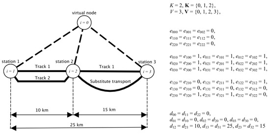
Figure 1. Illustration of a very simple railway network.

Each station i, as a place where trains can stop, start, or finish their runs, has limited capacity $CA{P}_i$ restricting the number of trains which are allowed to dwell on there at the same time. Additionally, it is assumed that each train fits every slot at a station, and a single train may occupy only one station slot. A virtual station ($i=0$) can hold up to $CA{P}_0=TR$ trains.

4.3. Representation of Train Timetable

In the paper, the train transport is considered to handle the flow of people traveling between stations. Many time demands and restrictions are imposed on resources (trains) and infrastructure (railway network) involved in such transport. They are reflected in a timetable, which takes into account not only constraints resulting from the joint use of resources and infrastructure, as well as their availability, but also nationally oriented regulations, along with other technical limitations. The railway transport is organized as a set of $TR$ train runs (or trains) $\mathbf{TR}=\{1,2,\dots ,TR\}$ which have specified routes with distinguished origins, destinations, and stopping stations provided with departure and arrival times at each station.

More specifically, each train $p\in \mathbf{TR}$ consists of a set of stations and a connected available set of tracks. They are organized in routes denoted by ${\mathit{R}}_p^{\mathrm{T}}={[R_{p,i,j,k}^{\mathrm{T}}]}_{i,j\in \mathbf{V},k\in \mathbf{K}}$, where $R_{p,i,j,k}^{\mathrm{T}}=1(0)$ if train p goes from station i to j by track k (otherwise). The timetable determines when the train p arrives and departures at station i, which is a part of a route ${\mathit{R}}_p^{\mathrm{T}}$. The arrival and departure times of p at station i belonging to route ${\mathit{R}}_p^{\mathrm{T}}$ are denoted by $t_{i,p}^{\mathrm{ARR}}$, $t_{i,p}^{\mathrm{DEP}}$, respectively. Besides the virtual station $i=0$, some obvious relations among the times are valid, like every departure time at a station must be not less than the corresponding arrival time, and an arrival time of the consecutively visited station i specified in ${\mathit{R}}_p^{\mathrm{T}}$ must be not less than the departure time from the previous one. Moreover, maximal arrival $T_{i,p}^{\mathrm{ARR}}$ or departure $T_{i,p}^{\mathrm{DEP}}$ lateness are given for some stations. A minimal dwell time $T_{i,p}^{\mathrm{D}}$ is defined for each station i and train p. Zero dwell times mean no stops at stations. The maximal dwell time during the train run for each station (except station 0) is common and equal to $T^{\mathrm{DL}}$.

The timetable for train run p is represented by a tuple $T{T}_p^{\mathrm{G}}=<{\mathbf{R}}_p^{\mathrm{T}},{(t_{i,p}^{\mathrm{ARR}},t_{i,p}^{\mathrm{DEP}})}_{i\in \mathbf{V}}>$, which forms for all trains the original timetable denoted by ${\mathit{TT}}^{\mathrm{G}}={[T{T}_p^{\mathrm{G}}]}_{p\in \mathbf{TR}}$. The timetable is not valid if, for any train run, any station exceeds its capacity $CA{P}_i$ (see Formula (7)). For stations that do not belong to the train route, all arrival and departure times are equal 0.

4.4. Representation of Track Closures

Some maintenance tasks of a railway infrastructure require track closures when no train is allowed to use servicing tracks. Consequently, track closures may affect timetables. Closures can be brought in periodically during a day or night for short periods, or they may be planned for longer periods: days, weeks, or even months. They can be assumed as a factor competing for a track possession together with train runs included in a timetable, as in Figure 2.

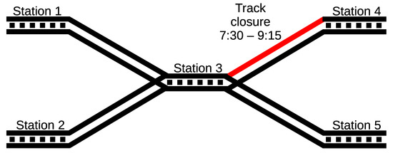
Figure 2. Illustration of an example of a track closure.

Let $\mathbf{C}=\{1,2,\dots ,C\}$ be a set of C track closures envisaged for the implementation. It is composed of $C^{\mathrm{OB}}$ obligatory closures and $C-C^{\mathrm{OB}}$ optional closures, i.e., $\mathbf{C}=\{1,2,\dots ,C^{\mathrm{OB}},C^{\mathrm{OB}}+1,C^{\mathrm{OB}}+2,\dots ,C\}$. The obligatory closures have to be included in the maintenance plan, unlike latter ones, which can be discarded if they interfere greatly the original timetable. An individual closure $n\in \mathbf{C}$ is defined by a tuple $S_n^G=<{\mathbf{R}}_n^{\mathrm{C}},t_n^{\mathrm{CES}},t_n^{\mathrm{CLS}},T_n^{\mathrm{C}}>$. All closures information is gathered in ${\mathbf{S}}^{\mathrm{G}}={[S_n^G]}_{n\in \mathbf{C}}$. A binary symmetric matrix ${\mathbf{R}}_n^{\mathrm{C}}={[R_{n,i,j,k}^{\mathrm{C}}]}_{i,j\in \mathbf{V},k\in \mathbf{K}\backslash \{0\}}$ informs on track possessions by closures, i.e., the current entry $R_{n,i,j,k}^{\mathrm{C}}=1(0)$ if track k between stations i and j is planned to be possessed by the nth track closure (otherwise). Other elements of the tuple comprise time information on closure n that is $T_n^{\mathrm{C}}$, $t_n^{\mathrm{CES}}$ and $t_n^{\mathrm{CLS}}$ represent, respectively, its duration, the earliest starting time and the latest starting time. If parameters $t_n^{\mathrm{CES}}$ and $t_n^{\mathrm{CLS}}$ have the same value, the start time of the closure is firm. Otherwise, it can vary between those two values. Moreover, closures may exist which have to be performed according to a given order expressed by a matrix $\mathit{O}={[o_{n,m}]}_{n,m\in \mathbf{C}}$, where $o_{n,m}=1(0)$ if closure n has to be completed directly before launching closure m.

4.5. Mathematical Model

At first, sub-problems of track closure planning and train rescheduling together with their mathematical models are separately introduced in Section 4.5.1 and Section 4.5.2, respectively. Then, in Section 4.5.3, the joint problem is stated in the form of the corresponding mathematical model as the composition of the models of sub-problems. All optimization (decision) variables defined in this subsection is summarized in Table 4. Their verbal descriptions are only given in this subsection.

Table 4. Decision variables.

Symbol	Description	Symbol	Description
$\mathit{y}$	binary matrix of closure planning	$\Delta t_{i,p}^{\mathrm{ARR}}\in \mathbb{N}$	element of $\Delta {\mathit{t}}^{\mathrm{ARR}}$ representing time shift of train p arrival to station i
$y_n\in \{0,1\}$	element of $\mathit{y}$ indicating the status of closure n	$\mathbf{\Delta }{\mathit{t}}^{\mathrm{DEP}}$	matrix with time shifts of train departures from stations
$\mathbf{\Delta }{\mathit{t}}^{\mathrm{C}}$	matrix with time shifts of closure start moments	$\mathit{S}$	matrix representing the plan of track closures
$\Delta t_n^{\mathrm{C}}\in \mathbb{N}$	element of $\mathbf{\Delta }{\mathit{t}}^{\mathrm{C}}$ representing the start time shift of closure n	$S_n$	element of S representing plan for closure n
${\mathit{r}}^{\mathrm{T}}$	matrix describing routes of all trains	$r_n^{\mathrm{C}}$	tracks to be closed during closure n
${\mathit{r}}_p^{\mathrm{T}}$	matrix describing the route of train p being the element of ${\mathit{r}}^{\mathrm{T}}$	$\mathit{TT}$	vector with timetable of trains
$r_{p,i,j,k}^{\mathrm{T}}\in \{0,1\}$	element of ${\mathit{r}}_p^{\mathrm{T}}$ describing the connection between stations i and j is used in the route of train p	$T{T}_p$	element of $\mathit{TT}$ given by a tuple representing the timetable of train p
$\mathbf{\Delta }{\mathit{t}}^{\mathrm{ARR}}$	matrix with time shifts of train arrivals to stations	$\mathit{x}$	binary matrix describing inclusion of trains into timetable $\mathit{TT}$
$\Delta t_{i,p}^{\mathrm{DEP}}\in \mathbb{N}$	element of $\mathbf{\Delta }{\mathit{t}}^{\mathrm{DEP}}$ representing time shift of train p departure from station i	$x_p\in \{0,1\}$	element of $\mathit{x}$ indicating the possible inclusion of train p into timetable $\mathit{TT}$

4.5.1. Track Closure Planning

The problem of track closure planning deals with finding of the possibly largest set of track closures (containing all obligatory closures) with fixed start times of closures that can be performed without interfering with a train run timetable. To this end, a binary decision vector $\mathit{y}={[y_n]}_{n\in \mathbf{C}}$ responsible for the planning of closures is introduced, where $y_n=1(0)$ if the nth closure is selected for the execution (otherwise). A positive-valued time shift (shift) of the closure earliest starting time $\mathbf{\Delta }{\mathit{t}}^{\mathrm{C}}={[\Delta t_n^{\mathrm{C}}]}_{n\in \mathbf{C}}$ is the second decision variable for planning the track closures. When the time shift is determined, the closure must start at the earliest starting time plus shift. Decision variables $\mathbf{\Delta }{\mathit{t}}^{\mathrm{C}}$ and $\mathit{y}$ define the resulted track closure plan $\mathit{S}={[S_n]}_{n\in \mathbf{C}}$, where $S_n=<R_{n,i,j,k}^{\mathrm{C}}·y_n,max\{t_n^{\mathrm{CES}},t_n^{\mathrm{CES}}+\Delta t_n^{\mathrm{C}}\},min\{t_n^{\mathrm{CLS}},t_n^{\mathrm{CLS}}+\Delta t_n^{\mathrm{C}}\},T_n^{\mathrm{C}}>$, and have to satisfy the constraints concerning obligatoriness, disjointness, and starting times of closures (see Formulas (2)–(4)). The track closure planning has to take into account the existing train timetable, which can affect likely conflicts in the track possessions by trains and closures.

4.5.2. Train Rescheduling

In fact, the train rescheduling deals with the elaboration of decision variables in the form of a new route plan ${\mathit{r}}^{\mathrm{T}}={[r_p^{\mathrm{T}}]}_{p\in \mathbf{TR}}$, ${\mathit{r}}_p^{\mathrm{T}}={[r_{p,i,j,k}^{\mathrm{T}}]}_{i,j\in \mathbf{V},k\in \mathbf{K}}$, where $r_{p,i,j,k}^{\mathrm{T}}=1(0)$ if train p is planned to run by track k between stations i and j (otherwise). Moreover, arrival time shifts $\Delta t_{i,p}^{\mathrm{ARR}}$ and departure time shifts $\Delta t_{i,p}^{\mathrm{DEP}}$ constitute the respective matrices of decision variables $\mathbf{\Delta }{\mathit{t}}^{\mathrm{ARR}}={[\Delta t_{i,p}^{\mathrm{ARR}}]}_{i\in \mathbf{V},p\in \mathbf{TR}}$ and $\mathbf{\Delta }{\mathit{t}}^{\mathrm{DEP}}={[\Delta t_{i,p}^{\mathrm{DEP}}]}_{i\in \mathbf{V},p\in \mathbf{TR}}$, as well as a new timetable $\mathit{TT}={[T{T}_p]}_{p\in \mathbf{TR}}$, where $T{T}_p=<{\mathit{r}}_p^{\mathrm{T}},{(t_{i,p}^{\mathrm{ARR}}+\Delta t_{i,p}^{\mathrm{ARR}},t_{i,p}^{\mathrm{DEP}}+\Delta t_{i,p}^{\mathrm{DEP}})}_{i\in \mathbf{V}}>$ is a new timetable for train run p. Both time shifts, together with the arrival and departure times from the original timetable ${\mathit{TT}}^{\mathrm{G}}$, define new arrival and departure times. The existence of some planned closures, unknown while preparing the original timetable ${\mathit{TT}}^{\mathrm{G}}$, is the only reason for rescheduling that is for the elaboration of a new timetable $\mathit{TT}$. No other unexpected events justifying possible rescheduling are taken into account in this paper. The considered track closures may directly affect train runs by their delaying, accelerating, or even canceling. The latter possibility is expressed in the model by an auxiliary decision variable $\mathit{x}={[x_p]}_{p\in \mathbf{TR}}$ influencing $\mathit{TT}$ by constraint (see Formula (9), where $x_p=1(0)$ if the pth train run is present in the new timetable (otherwise). It is important to point out that some train runs denoted by $\mathbf{T}{\mathbf{R}}^{\mathrm{OB}}\subseteq \mathbf{TR}$ may exist and have to be obligatorily inserted into $\mathit{TT}$. The train rescheduling has to obey some regulations on any train travel time extensions concerning timetable ${\mathit{TT}}^{\mathrm{G}}$. They assure that the total travel time extension cannot exceed the given limit $T^{\mathrm{E}}$, and the travel time extension on a given distance $D^{\mathrm{L}}$ cannot exceed the given limit $T^{\mathrm{DE}}$ (see Formulas (10) and (11)).

The matrices ${\mathit{r}}^{\mathrm{T}}$, $\mathbf{\Delta }{\mathit{t}}^{\mathrm{ARR}}$, $\mathbf{\Delta }{\mathit{t}}^{\mathrm{DEP}}$, and $\mathit{x}$, or equivalently $\mathit{TT}$, comprise all decisions made while rescheduling of trains.

4.5.3. Final Model and Its Analysis

Two groups of decisions $\mathit{y}$, $\mathbf{\Delta }{\mathit{t}}^{\mathrm{C}}$, as well as $\mathit{TT}$, together with $\mathit{x}$ introduced in two previous sub-sections, are mutually dependent. The plan of track closures $\mathit{y}$, $\mathbf{\Delta }{\mathit{t}}^{\mathrm{C}}$ usually entails changes in the timetable ${\mathit{TT}}^{\mathrm{G}}$, like the cancellation of trains and the shift of departure and (or) arrival times at stations. On the other hand, it is necessary to bear in mind strong limitations that are imposed on the plan of track closures by the original timetable ${\mathit{TT}}^{\mathrm{G}}$ being the basis and the source of technical restrictions for $\mathit{TT}$. So, the claim is entitled that $\mathbf{\Delta }{\mathit{t}}^{\mathrm{C}}$ and $\mathit{y}$ directly influences $\mathit{TT}$, and the indirect opposite impact is also valid, which forces the joint making of both groups of decisions $\mathbf{\Delta }{\mathbf{t}}^{\mathrm{C}}$, $\mathit{y}$ and $\mathit{TT}$. In the paper, the decisions are taken in the time horizon limited to the interval $[0,T^{\mathrm{H}}]$, where $T^{\mathrm{H}}=max(\underset{i\in \mathbf{V},p\in \mathbf{TR}}{max}{t}_{i,p}^{\mathrm{ARR}}+T^{\mathrm{E}},\underset{n\in \mathbf{C}}{max}(t_n^{\mathrm{CLS}}+T_n^{\mathrm{C}}))$ is the greater of times: the latest possible arrival of a train to the destination railway station according to the timetable ${\mathit{TT}}^{\mathrm{G}}$ and the greatest completion time of all the possible closures. All mentioned and resulted time variables have to belong to this interval. However, time shifts $\Delta t_{i,p}^{\mathrm{ARR}}$ and $\Delta t_{i,p}^{\mathrm{DEP}}$ can be negative.

To achieve a feasible solution, the following constraints are imposed on the decision variables:

–

all obligatory closures are performed (1),

–

all closure starting times are feasible (2),

–

every pair of closures has to be disjoint (3),

–

obligatory train runs from set ${\mathbf{TR}}^{\mathrm{OB}}$ are present in the new timetable (4),

–

run times between adjacent stations are fixed (5),

–

substitute transport is allowable for selected paths specified in matrix E and only possible if other tracks are not free (6),

–

capacities of stations are limited (only in artificial station ‘0’ capacity is unlimited) (7),

–

at most one train can occupy one track at every time moment (8),

–

the train cannot run by any track if it is canceled (9),

–

the total travel time extension cannot exceed the given limit $T^{\mathrm{E}}$ (10),

–

the travel time extension on a given distance $D^{\mathrm{L}}$ cannot exceed the given limit $T^{\mathrm{DE}}$ (11),

–

standing times of trains at stations are limited by the minimum and maximum feasible values (12),

–

trains in both original and new timetables go through the same path of stations, but they may go through different tracks (13),

–

departure and arrival lateness at selected stations are bounded (14),

–

the arrival time of every train at every station must not be later than corresponding departure time (15), and

–

no train can occupy a track during a closure (16).

Constraints imposed on track closures:

$$y_n=1,n=1,2,\dots ,C^{\mathrm{OB}},$$

(1)

$$t_n^{\mathrm{CES}}+\Delta t_n^{\mathrm{C}}\le t_n^{\mathrm{CLS}}+M(1-y_n),\Delta t_n^{\mathrm{C}}\ge 0,n\in \mathbf{C},$$

(2)

$$\begin{array}{c}min\{y_n(t_n^{\mathrm{CES}}+\Delta t_n^{\mathrm{C}}+T_n^{\mathrm{C}}),y_m(t_m^{\mathrm{CES}}+\Delta t_m^{\mathrm{C}}+T_m^{\mathrm{C}})\}\le max\{y_n(t_n^{\mathrm{CES}}+\Delta t_n^{\mathrm{C}}),y_m(t_m^{\mathrm{CES}}+\Delta t_m^{\mathrm{C}})\},\hfill \\ \hfill (n,m)\in {\mathbf{C}}^{\mathrm{CON}}=\{(n,m)\in \mathbf{C}\times \mathbf{C}:n\ne m,{\exists }_{i,j\in \mathbf{V},k\in \mathbf{K}}(R_{n,i,j,k}^{\mathrm{C}}+R_{m,i,j,k}^{\mathrm{C}}=2)\}.\end{array}$$

(3)

Constraints imposed on train runs:

$$x_p=1,p\in {\mathbf{TR}}^{\mathrm{OB}}.$$

(4)

Constraints imposed on train routes:

$$\sum _{k\in \mathbf{K}}(R_{p,i,j,k}^{\mathrm{T}}-r_{p,i,j,k}^{\mathrm{T}})(\Delta t_{j,p}^{\mathrm{ARR}}-\Delta t_{i,p}^{\mathrm{DEP}})=0,i,j\in \mathbf{V},p\in \mathbf{TR},$$

(5)

$$\begin{array}{c}{x}_p{r}_{p,i,j,0}^{\mathrm{T}}\le min\{e_{i,j,0},\frac{1+{\displaystyle \sum _{k\in \mathbf{K}\backslash \{0\}}}({\displaystyle \sum _{q\in {\mathbf{TR}}_{i,j,p}^{\mathrm{CON}}}}{x}_q{r}_{q,i,j,k}^{\mathrm{T}}+{\displaystyle \sum _{q\in {\mathbf{TR}}_{j,i,p}^{\mathrm{CON}}}}{r}_{q,j,i,k}^{\mathrm{T}}{x}_q+{\displaystyle \sum _{n\in {\mathbf{C}}_{i,j,p}^{\mathrm{CON}}}}{r}_{n,i,j,k}^{\mathrm{C}}{y}_n)}{(1+{\displaystyle \sum _{k\in \mathbf{K}\backslash \{0\}}}{e}_{i,j,k})}\},\hfill \\ \hfill i,j\in \mathbf{V},p\in \mathbf{TR},\end{array}$$

(6)

$$\begin{array}{c}{\mathbf{TR}}_{i,j,p}^{\mathrm{CON}}\stackrel{\Delta }{=}\{r\in \mathbf{TR}\backslash \{p\}:t_{i,p}^{\mathrm{DEP}}+\Delta t_{i,p}^{\mathrm{DEP}}\le t_{i,r}^{\mathrm{DEP}}+\Delta t_{i,r}^{\mathrm{DEP}}\le t_{j,p}^{\mathrm{ARR}}+\Delta t_{j,p}^{\mathrm{ARR}}\vee t_{i,r}^{\mathrm{DEP}}+\Delta t_{i,r}^{\mathrm{DEP}}\hfill \\ \hfill \le t_{i,p}^{\mathrm{ARR}}+\Delta t_{i,p}^{\mathrm{ARR}}\le \Delta t_{i,r}^{\mathrm{ARR}}+\Delta t_{i,r}^{\mathrm{ARR}}\},\end{array}$$

$$\begin{array}{c}{\mathbf{C}}_{i,j,p}^{\mathrm{CON}}\stackrel{\Delta }{=}\{n\in \mathbf{C}:t_{i,p}^{\mathrm{DEP}}+\Delta t_{i,p}^{\mathrm{DEP}}\le t_n^{\mathrm{CES}}+\Delta t_n^{\mathrm{C}}\le t_{j,p}^{\mathrm{ARR}}+\Delta t_{j,p}^{\mathrm{ARR}}\vee t_n^{\mathrm{CES}}+\Delta t_n^{\mathrm{C}}\hfill \\ \hfill \le t_{i,p}^{\mathrm{ARR}}+\Delta t_{i,p}^{\mathrm{ARR}}\le t_n^{\mathrm{CES}}+\Delta t_n^{\mathrm{C}}+T_n^{\mathrm{C}}\},\end{array}$$

$$\begin{array}{c}\sum _{j\in \mathbf{V}}\sum _{k\in \mathbf{K}\backslash \{0\}}{x}_{p}max(r_{p,j,i,k}^{\mathrm{T}},r_{p,i,j,k}^{\mathrm{T}})(1+\sum _{q\in {\mathbf{TR}}_{i,p}^{\mathrm{CON}}}\sum _{l\in \mathbf{V}}\sum _{m\in \mathbf{K}\backslash \{0\}}{x}_{q}max(r_{q,i,l,m}^{\mathrm{T}},r_{q,l,i,m}^{\mathrm{T}})\le CA{P}_i,\hfill \\ \hfill i\in \mathbf{V}\backslash \{0\},p\in \mathbf{TR},\end{array}$$

(7)

$$\begin{array}{c}min\{r_{p,i,j,k}^{\mathrm{T}}{x}_p(t_{i,p}^{\mathrm{DEP}}+\Delta t_{i,p}^{\mathrm{DEP}})+r_{p,j,i,k}^{\mathrm{T}}{x}_p(t_{i,p}^{\mathrm{ARR}}+\Delta t_{i,p}^{\mathrm{ARR}}),\hfill \\ r_{q,i,j,k}^{\mathrm{T}}{x}_q(t_{j,q}^{\mathrm{ARR}}+\Delta t_{j,q}^{\mathrm{ARR}})+r_{q,j,i,k}^{\mathrm{T}}{x}_q(t_{i,q}^{\mathrm{ARR}}+\Delta t_{i,q}^{\mathrm{ARR}})\}\\ \le max\{r_{p,i,j,k}^{\mathrm{T}}{x}_p(t_{i,p}^{\mathrm{DEP}}+\Delta t_{i,p}^{\mathrm{DEP}})+r_{p,j,i,k}^{\mathrm{T}}{x}_p(t_{j,p}^{\mathrm{DEP}}+\Delta t_{j,p}^{\mathrm{DEP}}),\\ r_{q,i,j,k}^{\mathrm{T}}{x}_q(t_{i,q}^{\mathrm{DEP}}+\Delta t_{i,q}^{\mathrm{DEP}})+r_{q,j,i,k}^{\mathrm{T}}{x}_q(t_{j,q}^{\mathrm{DEP}}+\Delta t_{j,q}^{\mathrm{DEP}})\},\\ r_{p,i,j,k}^{\mathrm{T}}(t_{i,p}^{\mathrm{DEP}}+\Delta t_{i,p}^{\mathrm{DEP}})\le r_{p,i,j,k}^{\mathrm{T}}(t_{j,p}^{\mathrm{ARR}}+\Delta t_{j,p}^{\mathrm{ARR}}),\\ \hfill p,q\in \mathbf{TR},i,j\in \mathbf{V},k\in \mathbf{K}\backslash \{0\}.\end{array}$$

(8)

Constraint imposed on train run times:

$$r_{p,i,j,k}^{\mathrm{T}}\le x_p,p\in \mathbf{TR},i,j\in \mathbf{V},k\in \mathbf{K},$$

(9)

$$(\Delta t_{0,p}^{\mathrm{ARR}}-\Delta t_{0,p}^{\mathrm{DEP}})·x_p\le T^{\mathrm{E}},p\in \mathbf{TR},$$

(10)

$$(\Delta t_{j,p}^{\mathrm{DEP}}-\Delta t_{i,p}^{\mathrm{ARR}})·x_p\le T^{\mathrm{DE}},(i,j)\in {\mathbf{D}}_p^{\mathrm{L}},p\in \mathbf{TR},$$

(11)

$$T_{i,p}^{\mathrm{D}}\le t_{i,p}^{\mathrm{DEP}}+\Delta t_{i,p}^{\mathrm{DEP}}-(t_{i,p}^{\mathrm{ARR}}+\Delta t_{i,p}^{\mathrm{ARR}})\le T^{\mathrm{DL}},i\in \mathbf{V},p\in \mathbf{TR},$$

(12)

$$\sum _{k\in \mathbf{K}}{R}_{p,i,j,k}^{\mathrm{T}}=\sum _{k\in \mathbf{K}}{r}_{p,i,j,k}^{\mathrm{T}},i,j\in \mathbf{V},p\in \mathbf{TR},$$

(13)

$$\Delta t_{i,p}^{\mathrm{DEP}}\le T_{i,p}^{\mathrm{DEP}},\Delta t_{i,p}^{\mathrm{ARR}}\le T_{i,p}^{\mathrm{ARR}},i\in \mathbf{V},p\in \mathbf{TR},$$

(14)

$$t_{i,p}^{\mathrm{ARR}}+\Delta t_{i,p}^{\mathrm{ARR}}\le t_{i,p}^{\mathrm{DEP}}+\Delta t_{i,p}^{\mathrm{DEP}},i\in \mathbf{V}\backslash \{0\},p\in \mathbf{TR}.$$

(15)

Constraint imposed on both train runs and track closures:

$$\begin{array}{c}min\{r_{p,i,j,k}^{\mathrm{T}}{x}_p(t_{j,p}^{\mathrm{ARR}}+\Delta t_{j,p}^{\mathrm{ARR}}),y_n(t_n^{\mathrm{CES}}+\Delta t_n^{\mathrm{C}}+T_n^{\mathrm{C}})\}\le max\{r_{p,i,j,k}^{\mathrm{T}}{x}_p(t_{i,p}^{\mathrm{DEP}}+\Delta t_{i,p}^{\mathrm{DEP}}),y_n(t_n^{\mathrm{CES}}+\Delta t_n^{\mathrm{C}})\},\hfill \\ \hfill p\in \mathbf{TR},n\in \mathbf{C},i,j\in \mathbf{V},k\in \mathbf{K}\backslash \{0\}:r_{n,i,j,k}^{\mathrm{C}}=1.\end{array}$$

(16)

The auxiliary notions used in (17) and (16) have the following meanings: M—big number,

• ${\mathbf{C}}^{\mathrm{CON}}=\{(n,m)\in \mathbf{C}\times \mathbf{C}:n\ne m,{\exists }_{i,j\in \mathbf{V},k\in \mathbf{K}}(R_{n,i,j,k}^{\mathrm{C}}+R_{m,i,j,k}^{\mathrm{C}}=2)\}$—set of closures reporting possession of the same track,
• ${\mathbf{TR}}_{i,p}^{\mathrm{CON}}=\{q\in \{1,2,\dots ,TR\}:t_{i,p}^{\mathrm{ARR}}\le t_{i,q}^{\mathrm{DEP}}\le t_{i,p}^{\mathrm{DEP}}\vee t_{i,p}^{\mathrm{ARR}}\le t_{i,q}^{\mathrm{ARR}}\le t_{i,p}^{\mathrm{DEP}}\}$—sub-set of trains with dwell time on the station i coinciding with that of the train run p,
• ${\mathbf{TR}}_{i,j,p}^{\mathrm{CON}}\stackrel{\Delta }{=}\{r\in \mathbf{TR}\backslash \{p\}:t_{i,p}^{\mathrm{DEP}}+\Delta t_{i,p}^{\mathrm{DEP}}\le t_{i,r}^{\mathrm{DEP}}+\Delta t_{i,r}^{\mathrm{DEP}}\le t_{j,p}^{\mathrm{ARR}}+\Delta t_{j,p}^{\mathrm{ARR}}\vee t_{i,r}^{\mathrm{DEP}}+\Delta t_{i,r}^{\mathrm{DEP}}\le t_{i,p}^{\mathrm{ARR}}+\Delta t_{i,p}^{\mathrm{ARR}}$$\le \Delta t_{i,r}^{\mathrm{ARR}}+\Delta t_{i,r}^{\mathrm{ARR}}\}$—sub-set of train runs going from i to j in time coincided with the run of train p,
• ${\mathbf{C}}_{i,j,p}^{\mathrm{CON}}\stackrel{\Delta }{=}\{n\in \mathbf{C}:t_{i,p}^{\mathrm{DEP}}+\Delta t_{i,p}^{\mathrm{DEP}}\le t_n^{\mathrm{CES}}+\Delta t_n^{\mathrm{C}}\le t_{j,p}^{\mathrm{ARR}}+\Delta t_{j,p}^{\mathrm{ARR}}\vee t_n^{\mathrm{CES}}+\Delta t_n^{\mathrm{C}}\le t_{i,p}^{\mathrm{ARR}}+\Delta t_{i,p}^{\mathrm{ARR}}\le t_n^{\mathrm{CES}}+\Delta t_n^{\mathrm{C}}+T_n^{\mathrm{C}}\}$—sub-set of track closures on the path from i to j in time coincided with the run of train p,
• ${\mathbf{TR}}_{i,p}^{\mathrm{CON}}=\{q\in \{1,2,\dots ,TR\}:t_{i,p}^{\mathrm{ARR}}+\Delta t_{i,p}^{\mathrm{ARR}}\le t_{i,q}^{\mathrm{DEP}}+\Delta t_{i,q}^{\mathrm{DEP}}\le t_{i,p}^{\mathrm{DEP}}+\Delta t_{i,p}^{\mathrm{DEP}}\vee t_{i,p}^{\mathrm{ARR}}+\Delta t_{i,p}^{\mathrm{ARR}}\le t_{i,q}^{\mathrm{ARR}}+\Delta t_{i,q}^{\mathrm{ARR}}$$\le t_{i,p}^{\mathrm{DEP}}+\Delta t_{i,p}^{\mathrm{DEP}}\}$—sub-set of train runs waiting at station i in time coincided with the run of train p,
• ${\mathbf{D}}_p^{\mathrm{L}}=\{(i,j)\in {\mathbf{TR}}^2:D^{\mathrm{L}}-r_{p,j,i(l),k}^{\mathrm{T}}·d_{j,i(l)}\ge r_{p,i,i1,k}^{\mathrm{T}}·d_{i,i1}+r_{p,i1,i2,k}^{\mathrm{T}}·d_{i1,i2}+\dots +r_{p,i(l-1),j,k}^{\mathrm{T}}·d_{i(l-1),j}<D^{\mathrm{L}}\}$—set of stations, for which train run p runs a distance less than $D^{\mathrm{L}}$, but it will reach or exceed this value on arrival to the next station.

Many interconnections between two groups of decisions $\mathbf{\Delta }{\mathit{t}}^{\mathrm{C}}$, $\mathit{y}$, and $\mathit{TT}$ are also visible while analyzing the constraints, e.g., (16). They are the additional justification for joint determination of both groups of decisions.

To evaluate the decisions $\mathit{y}$, $\mathbf{\Delta }{\mathit{t}}^{\mathrm{C}}$, as well as $\mathit{TT}$, the following criterion is proposed:

$$Q=\alpha {\sum }_{n=C^{\mathrm{OB}}+1}^C{y}_n+\sum _{p\in \mathbf{TR}\backslash {\mathbf{TR}}^{\mathrm{OB}}}{x}_p-\beta \sum _{i\in \mathbf{V},p\in \mathbf{TR}}\left|\Delta {\tau }_{i,p}^{DEP},\right|,$$

(17)

where $\alpha$ and $\beta$ are positive-valued coefficients satisfying the inequalities $\alpha >TR-T{R}^{\mathrm{OB}},\beta <1/[TR(V+1)T^{\mathrm{H}}]$, e.g., $\alpha =TR-T{R}^{\mathrm{OB}}+1,\beta =1/[TR(V+1)T^{\mathrm{H}}+1]$.

The introduced criterion reflects the Polish Railways expectations. The most important is to perform as many closures as possible, since they are crucial for maintenance of railway tracks and affect the long-term rail traffic management. Thus, the first element of (17) evaluate number of closures which are to be performed according to the solution. The $\alpha$ parameter chosen according to the imposed constraint ensures that every closure is more important than any acceptable change in timetable. While we cannot increase the number of closures, we should try to limit the number of the train runs that are to be canceled. Thus, the second element of (17) evaluates number of train runs which remain in the new timetable. The $\beta$ parameter chosen according to the given constraint provides that not canceling any train run is more important than introducing any changes in the departure times in the new timetable. At last, when we can increase neither the number of closures nor the number of train runs, we should try to minimize the total time changes in the new timetable, which is reflected by the last element of the objective function. Such form of the criterion ensures the hierarchy of the decisions, i.e., the acceptance of optional closures is the most important, whereas the differences of departure times in the timetables are the least important.

To sum up, the following joint train rescheduling and track closure planning problem is considered and solved. Decisions are made in relation to the railway system which consists of a railway infrastructure and train runs described by $\mathbf{G}$, $\mathbf{V}$, $\mathbf{TR}$, $\mathbf{T}{\mathbf{R}}^{\mathrm{OB}}$, ${\mathit{TT}}^{\mathrm{G}}$, $\mathit{D}$, $CA{P}_i$, $T_{i,p}^{\mathrm{ARR}}$, $T_{i,p}^{\mathrm{DEP}}$, $T_{i,p}^{\mathrm{D}}$, $i,j\in \mathbf{V}$, $p\in \mathbf{TR}$, $\alpha$,$\beta$. The planned closures are also given in the form of $\mathbf{C}$, C, $C^{\mathrm{OB}}$, $\mathit{O}$, ${\mathit{S}}^{\mathrm{G}}({\mathit{S}}_n=<{\mathit{R}}_n^{\mathrm{C}},t_n^{\mathrm{CES}},t_n^{\mathrm{CLS}},T_n^{\mathrm{C}}>,n\in \mathbf{C})$. The auxiliary data $T^{\mathrm{DL}}$, $T^{\mathrm{DE}}$, $T^{\mathrm{E}}$ are known, as well. It is necessary to determine the interconnected collection of decisions: $\mathbf{\Delta }{\mathit{t}}^{\mathrm{C}}$, $\mathit{y}$ constituting the resulted track closure plan, and ${\mathit{r}}^{\mathrm{T}}$,$\Delta {\mathit{t}}^{\mathrm{ARR}}$, $\mathbf{\Delta }{\mathit{t}}^{\mathrm{DEP}}$, $\mathit{x}$ defining the new timetable plan $\mathit{TT}$ subject to constraints (1)–(16) to minimize the criterion (17).

The conducted analysis of the formulated nonlinear mixed integer optimization problem referred to as PR made it possible to put forward and prove the following theorem.

Theorem 1.

Joint train rescheduling and track closure planning problem is NP-hard.

Proof. 

Let us consider the NP-hard problem of task scheduling around a common date presented in Reference [62]. Given one executor and J tasks, durations of tasks $duratio{n}_j\ge 0,j=1,2,\dots ,J$ and a common deadline $deadline\le {\sum }_{j\in \{1,2,\dots ,J\}}duratio{n}_j$ find a schedule, i.e., task completion times $finis{h}_j$, that minimizes the total earliness and tardiness of each task, i.e., $quality={\sum }_{j\in \{1,2,\dots ,J\}}|finis{h}_j-deadline|$. We show that this scheduling problem reduces, in polynomial time, to the investigated problem PR. We accomplish this by showing that we can reduce the scheduling problem to an equivalent problem PR with only single track and carefully selected set of closures.

We take a time horizon sufficient to encompass the duration of all tasks ($T^{\mathrm{H}}={\sum }_{j}duratio{n}_j$). Let us assume that all closures and train runs are obligatory ($y_n=1,x_p=1$). Define the graph $\mathbf{G}$ so that there are 3 stations connected in a cycle $0\to 1\to 2\to 0$, and that there are $J+1$ tracks between stations 1 and 2. We take J trains, where each train moves once through the whole cycle of stations but through different track each: pth train takes pth track between stations 1 and 2 ($R_{p,0,1,1}^{\mathrm{T}}=1$, $R_{p,1,2,p}^{\mathrm{T}}=1$, $R_{p,2,0,1}^{\mathrm{T}}=1$). The departure time for the artificial station is 0 for every train and so is the arrival in station 1. Departure time in station 1, as well as minimum dwelling time, is set to $deadline-duratio{n}_j$. Arrival time in station 2 for the pth train is equal to $deadline$. Minimum dwelling time in station 2 is 0. Maximal dwell times are set to be very large ($T^{\mathrm{DL}}=T^{\mathrm{H}}$). Note that the schedule is feasible.

Let us further consider a set of J closures, where the nth closure takes up track n of the connection between stations 1 and 2 ($R_{n,1,2,n}^{\mathrm{C}}=1$) with the earliest and the latest start times all bound by 0 and very large durations ($t_n^{\mathrm{CES}}=t_n^{\mathrm{CLS}}=0$,$T_n^{\mathrm{C}}=T^{\mathrm{H}}$). The addition of closures forces all the trains onto the last track $J+1$, where they cannot proceed in parallel. Due to dwelling times in station 2, the quality criterion is equal to $Q={\sum }_{j\in \{1,2,\dots ,J\}}|\Delta t_{1,j}^{\mathrm{DEP}}|+{\sum }_{j\in \{1,2,\dots ,J\}}|\Delta t_{2,j}^{\mathrm{DEP}}|=2{\sum }_{j\in \{1,2,\dots ,J\}}|\Delta t_{2,j}^{\mathrm{DEP}}|=2{\sum }_{j\in \{1,2,\dots ,J\}}|t_{2,j}^{\mathrm{DEP}}+\Delta t_{2,j}^{\mathrm{DEP}}-deadline|$.

Sum $t_{2,j}^{\mathrm{DEP}}+\Delta t_{2,j}^{\mathrm{DEP}}$ is the moment the train run ends. Thus, we equate it to $finis{h}_j$. Then, $quality=\frac{1}{2}Q$. Please note that all the transformations can be made in the polynomial time. □

5. Heuristic Solution Algorithm

The optimization problem PR formulated in the previous section should be solved in a reasonable amount of time. For example in Poland, at least a single feasible solution is required within 48 h. It is very tough to fulfill such requirements due to the NP-hardness of PR, as well as its non-linearity and the huge dimension with respect both to the number of variables and to the number of constraints. The whole Polish railway network there is represented by over ${10}^{12}$ binary and ${10}^8$ integer variables. The transformation of the considered problem into MIP using ’big M’ to solve it by a known solver failed. It resulted in the enormous growth of the problem’s dimension, and, in consequence, the approach turned out useless due to the non-acceptable computation time. Another considered approach assumed the application of selected metaheuristics. It also failed as the significant calculation effort was mostly devoted to checking infeasible solutions. Unfortunately, there is no a simple method for the generation of any initial train runs timetable and a closure plan fulfilling all the constraints under consideration. The utmost case is possible for a metaheuristic-based solution algorithm when the feasible execution time can elapse before any solution is sought. Therefore, the problem-specific heuristic algorithm is proposed, which is based on some simplifications and decompositions neglecting some connections between variables and constraints. However, due to the complexity of the problem, the solution algorithm might not guarantee feasible solutions for some of the strongly constrained cases. The detailed presentation of the algorithm’s components in the subsequent sub-sections follows the overview of the algorithm.

A multi-level algorithm of the hierarchical parallel structure is proposed, as in Figure 3. There are four main levels of algorithms which are dependent on one another, i.e., an upper level algorithm requires (usually multiple) solutions of the lower level algorithm. Algorithm 1 is responsible for the selection of facultative closures. Algorithm 2 provides the selection of facultative train runs. Algorithm 3 is responsible for decomposition of the railway network into smaller, more manageable parts. This is done with the help of a separate Track Grouping Algorithm (TGA). Finally, Algorithm 4 is responsible for finding actual schedules under given closures, train runs and decomposition. Algorithm 4 itself is further divided into Algorithms 5, 6, and 7. Those sub-algorithms are run for every sub-network that was obtained with the use of Algorithm 3. Algorithm 1 sequentially approves individual closures for launching in such a way to ensure the generation of feasible timetables. The feasibility of a current closure is checked by all other algorithms. Algorithm 1 decides via $y_n$ on the inclusion of the current closure into the set of accepted closures according to information returned by Algorithm 2. However, it is necessary to cover all obligatory closures. On the analogous basis, Algorithm 2 using $\mathit{x}$ sequentially, i.e., one by one, forms the set of accepted trains for the new timetable. It takes into account information returned by Algorithm 3 which, in turn, is launched at every iteration of Algorithm 2. Algorithm 3 assumes the decomposition of a railway network performed by the Track Grouping Algorithm TGA into $\eta$ groups (railway sub-networks). For each sub-network, Algorithm 4 is launched to obtain train runs and track closures time shifts $\mathbf{\Delta }{\mathit{t}}^{\mathrm{ARR}}$, $\mathbf{\Delta }{\mathit{t}}^{\mathrm{DEP}}$, and $\mathbf{\Delta }{\mathit{t}}^{\mathrm{C}}$ for this fragment of the network. If rerouting is needed, then Algorithm 4 also returns the routes ${\mathit{r}}^{\mathrm{T}}$.

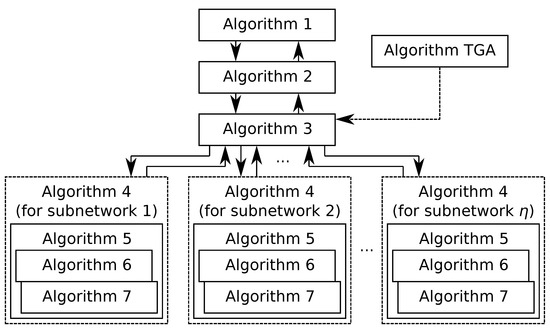
Figure 3. Structure of multi-level algorithm.

The following optimization tasks are performed by Algorithm 4 for every sub-network: a track order, a station order, and a time shift resolution, where first two tasks are Mixed Integer Linear Programming (MILP), while the last one is the Linear Programming (LP). All of them are iteratively solved with the combined use of a greedy algorithm and the numerical solver ‘lp_solve’ [63], giving solutions of resulted LP. As a consequence, the decision variables of the considered problem, i.e., $\mathit{y}$, $\mathit{x}$ and $\mathbf{\Delta }{\mathit{t}}^{\mathrm{C}}$, ${\mathit{r}}^{\mathrm{T}}$, $\mathbf{\Delta }{\mathit{t}}^{\mathrm{ARR}}$, $\mathbf{\Delta }{\mathit{t}}^{\mathrm{DEP}}$ are the results of Algorithms 1, 2, 3, 4, together with TGA, respectively. The matrices ${\mathit{r}}^{\mathrm{T}}$, $\mathbf{\Delta }{\mathit{t}}^{\mathrm{ARR}}$, $\mathbf{\Delta }{\mathit{t}}^{\mathrm{DEP}}$, along with $\mathit{x}$, form the new timetable $\mathit{TT}={[<x_p·{[r_{p,i,j,k}^{\mathbf{T}}]}_{i,j\in \mathbf{V},k\in \mathbf{K}},{[t_{i,p}^{\mathrm{ARR}}+\Delta t_{i,p}^{\mathrm{ARR}}]}_{i\in \mathbf{V}},{[t_{i,p}^{\mathrm{DEP}}+\Delta t_{i,p}^{\mathrm{DEP}}]}_{i\in \mathbf{V}}>]}_{p\in \mathbf{TR}}$. Similarly, the time shifts for closures $\mathbf{\Delta }{\mathit{t}}^{\mathrm{C}}$, together with $\mathit{y}$, define the resulted track closure plan $\mathit{S}={[S_n]}_{n\in \mathbf{C}}$, where $S_n=<r_n^{\mathrm{C}},t_n^{\mathrm{CSE}},t_n^{\mathrm{CSL}},T_n^{\mathrm{C}}>$, $r_n^{\mathrm{C}}=R_{n,i,j,k}^{\mathrm{C}}·y_n$, $t_n^{\mathrm{CSE}}=max\{t_n^{\mathrm{CES}},t_n^{\mathrm{CES}}+\Delta t_n^{\mathrm{C}}\}$, $t_n^{\mathrm{CSL}}=min\{t_n^{\mathrm{CLS}},t_n^{\mathrm{CLS}}+\Delta t_n^{\mathrm{C}}\}$.

Algorithms 1, 2, 3, 4 and TGA are introduced in the next subsections. The detailed description of Algorithm TGA can be found in Reference [5]. It is assumed that all algorithms have access to all data concerning infrastructure, train runs, and track closures. The necessary auxiliary notation is given in Table 5.

Table 5. Decision variables.

Notation Used in Algorithm 1
Symbol	Description	Symbol	Description
$r_n^{\mathrm{C}}$	tracks to be closed during closure n	${\mathbf{C}}^{\mathrm{OB}}$	set of obligatory closures
$t_n^{\mathrm{CE}}$	actual completion time of closure n	${\mathbf{C}}^{\mathrm{F}}$	set of facultative closures
$z_i$	sequence of obligatory closures	${\mathbf{C}}^{\mathrm{S}}$	set of selected closures to be passed to Algorithm 2
Notation Used in Algorithm 2
Symbol	Description	Symbol	Description
${\mathbf{TR}}^{\mathrm{S}}$	selected train runs to be passed to Algorithm 3	$W_{p,k}$	variable indicating the run of train p by track k between given stations
$\Delta$	parameter of Algorithm 2 representing the limit of time shifts of closures or trains	$U_p$	conflict index for the train run p
Notation Used in Algorithm 3
Symbol	Description	Symbol	Description
${\mathit{S}}^{\prime }$	temporary closure plan	${\mathbf{V}}_n$	set of stations of the decomposed sub-network n
${\mathit{TT}}^{\prime }$	temporary train timetable	$\eta$	number of sub-networks in the decomposition
$\mathbf{GR}$	set of track assignments to groups used for the decomposition	${\pi }_{n,p}$	string of stations representing the path of train p
$\mathbf{E}$	set of tuples describing each arc that exists in network $\mathbf{G}$	${\mathbf{C}}_n^{\mathrm{S}}$	set of closures in the decomposed sub-network n
${\mathbf{G}}_n$	graph representing the decomposed railway sub-network n.	${\mathbf{TR}}_n^{\mathrm{S}}$	set of trains in decomposed sub-network n
${\mathbf{E}}_n$	matrix of tracks (matrix extended by virtual tracks) for the decomposed sub-network n	q	train run marked for rerouting
Notation Used in Algorithm 4
Symbol	Description	Symbol	Description
${\mathsf{\Psi }}^{i,j,k}$	series of elements indicating tracks that have trains or track closures and their order	${\mathbf{C}}_{i,j,k}$	set of closures on the given track
${\mathsf{\Psi }}_m^{i,j,k}$	element of ${\mathsf{\Psi }}^{i,j,k}$ indicating if tracks have trains or track closures at position m	${\mathbf{TR}}_{i,j,k}$	set of trains going through track $(i,j,k)$
${\mathit{\theta }}^{i,j,k}$	matrix representing the order of track usage by either trains or closures	${\mathbf{TR}}_n^{\mathrm{S}\_\mathrm{SUB}}$	sub-set of ${\mathbf{TR}}_n^{\mathrm{S}}$,
${\theta }_m^{i,j,k}$	element of ${\mathit{\theta }}^{i,j,k}$	$Q_1^{i,j,k}$	total time shift for trains limited to a single track at a time
${\mathsf{\Theta }}^{i,j,k}$	number of trains and closures on track k connecting stations i and j	${\mathbf{TR}}_i$	set of trains on tracks adjacent to station i.
${\mathit{\lambda }}^i$	matrix representing the order of trains entering station i	${\mathbf{K}}_i^{\mathrm{ADJ}}$	set of tracks adjacent to station i.
${\lambda }_m^i$	element of ${\lambda }^i$ indicating number of train entering station i in the order m	$Q_2^i$	total time shift of trains for station i.
${\mathsf{\Lambda }}^i$	number of trains entering station i

5.1. Managing of Closures

Algorithm 1 checks serially the ordered sequences of obligatory and facultative closures. Each track closure n is numerically evaluated by the ratio

$$\frac{T_n^{\mathrm{C}}{R}_{n,i,j,k}^{\mathrm{C}}{\sum }_{p=1}^{TR}{R}_{p,i,j,k}^{\mathrm{T}}}{{\sum }_{k=1}^K{\sum }_{p=1}^{TR}(t_{j,p}^{\mathrm{ARR}}-t_{i,p}^{\mathrm{DEP}})R_{p,i,j,k}^{\mathrm{T}}}$$

(18)

being the proportion of daily cumulated time of the closure to a daily time occupation by trains in the original timetable ${\mathit{TT}}^{\mathrm{G}}$ of the trail between stations i and j. The cumulated time of closure is equal to time $T_n^{\mathrm{C}}$ multiplied by the number of trains using the track during $T_n^{\mathrm{C}}$. The trail is understood as all tracks between adjacent stations. Additionally, both sequences are sorted to take into account precedence constraints among closures given in matrix $\mathit{O}$. A closure is selected on the basis of the real-world completion time of closure $t_n^{\mathrm{CE}}$ returned by the lower level Algorithm 2. The non-positive returned value of $t_n^{\mathrm{CE}}$ means that some constraints do not hold, and closure n cannot be approved. Algorithm 1 is stopped when whichever obligatory closure cannot be performed. As a result, the algorithm returns the selected set of track closures, the set of train runs together with new train timetable and track closure plans obtained, or information that the solution does not exists. The returned set of train runs defined by $\mathit{x}$, together with train timetable $\mathit{TT}$ and a set of closures defined by $\mathit{y}$, together with closure plan $\mathit{S}$, are obtained with the use of all subsequent algorithms.

5.2. Managing of Train Runs

The management of train runs is performed by Algorithms 2 and 3 supported by Algorithm TGA, as well as by the solution of an auxiliary sub-problem ZP [64]. It is focused on obtaining such a sub-set of train runs, which enables the presence of a given set of track closures. If any obligatory train run cannot be included into the timetable due to a failing of constraints, information of the closure set infeasibility is returned to the track closure management part. The initial proposition of a train run set for the inclusion into the solution is obtained by Algorithm 2. This algorithm uses the decomposition procedure (Algorithm 3) to check if all suggested train runs could be performed, what is represented by a new train timetable and a new track closure plan. If Algorithm 3 fails to find a feasible timetable and a track closure plan, Algorithm 2 is stopped returning the last feasible train timetable and track closure plan with information if all obligatory train runs are included in this timetable.

Let us describe Algorithm 2 for indicating train runs to be placed into the new train timetable starting from the introduction of the following auxiliary variable $U_p=\frac{{\sum }_i{\sum }_j\left({\sum }_k{R}_{p,i,j,k}^{\mathrm{T}}\right)\left({\sum }_{q:[t_{i,p}^{\mathrm{ARR}},t_{j,p}^{\mathrm{DEP}}]\cap [t_{i,q}^{\mathrm{ARR}},t_{j,q}^{\mathrm{DEP}}]\ne \varnothing }1\right)}{{\sum }_i{\sum }_j{\sum }_k{R}_{p,i,j,k}^{\mathrm{T}}}$ referred to as conflicts index for the train run. The variable indicates how many other than p trains are located at the same time on the p’s train trail (or on the railway stations of this trail) in relation to the number of all tracks traveled by the pth train.

The usage of Algorithm 2 allows estimating whether it is likely to have a feasible solution of train rescheduling and track closure planning for the whole railway network when the new closure or the new train run is added. In consequence, Algorithm 2 uses the solution of the parameterized sub-problem ZP, for which the formal definition is given in Reference [64]. ZP limits the whole network to a single trail affected by the current change in the closure plan or the set of accepted train runs. This change is accomplished by assigning start times of closures and making train run timetable for this trail. The aim is to settle if we can shift closures and train runs by no more than a given period $\Delta$ (algorithm parameter), which eliminates conflicts. We also assume that each train run may change its track between considered stations, so the new track is indicated by the variable $W_{p,k}$.

Although ZP is a constraint satisfaction sub-problem, it may be easily solved by a linear programming solver, e.g., ‘lpsolve’ [63]. Notice that, even if the solution of the problem ZP can be found, it does not guarantee the existence of solution for the whole railway network.

Whenever Algorithm 3 is launched, it uses the results of Algorithm TGA, which takes $\mathbf{G}$, $\mathit{TT}$, and $\mathbf{TR}$ as an input and returns the number of groups $\eta$ and set $\mathbf{GR}=\mathbf{E}\times \{1,2,\dots \eta \}$, where $\mathbf{E}=\{(i,j,k):e_{i,j,k}=1\}$. The set $\mathbf{GR}$ represents the assignments of each track to a number corresponding to the index of one of the defined groups. Algorithm 3 divides the railway network into sub-networks and, after the grouping of all tracks, complements them with artificial ones. Artificial tracks connect stations which were not yet connected but are consecutive stations of some train run in its route. Then, for each sub-network, Algorithm 4 is consecutively executed to obtain a new timetable and a track closure plan corresponding to this fragment of the network. If, for all sub-networks, the feasible solution is found, then all results are combined into a single train timetable and track closure plan, as well as returned together with information about the success. Otherwise, the algorithm returns the original train timetable and track closure plan with information of the failure. The new train timetable $\mathit{TT}$ and track closure plan $\mathit{S}$ are represented by values of time shifts $\Delta {\mathit{t}}^{\mathrm{ARR}}$, $\Delta {\mathit{t}}^{\mathrm{DEP}}$ of train runs and time shifts $\Delta {\mathit{t}}^{\mathrm{C}}$ of track closures regarding the original timetable ${\mathbf{TR}}^{\mathrm{S}}$ and closure plan ${\mathbf{C}}^{\mathrm{S}}$.

Algorithm 1 selection of closures

Require: Data of the problem, in particular sets ${\mathbf{C}}^{\mathrm{OB}}$, ${\mathbf{C}}^{\mathrm{F}}$ of obligatory, facultative closures, respectively. Ensure: Values of $\mathit{y}$, $\mathit{x}$, as well as closure plan $\mathit{S}$, and timetable $\mathit{TT}$. 1: Sort the elements of ${\mathbf{C}}^{\mathrm{OB}}$ in the ascending order with respect to ratio (18) and then sort resulting sequence to ensure precedence constraints given in matrix $\mathit{O}$ to have a sequence of obligatory closures ${(z_i)}_{i=1,\dots ,{\mathrm{C}}^{\mathrm{OB}}}$ as a consequence. 2: Set $y_n=0$, $\Delta t_n^{\mathrm{C}}=0$, $n=1,2,\dots ,C$, $x_p=0$, $p\in \mathbf{TR}$, $\mathit{S}={\mathit{S}}^{\mathrm{G}}$, $\mathit{TT}={\mathit{TT}}^{\mathrm{G}}$. 3: for$i=1,\dots ,{\mathbf{C}}^{\mathrm{OB}}$do 4:       Run Algorithm 2 for a set of selected closures ${\mathbf{C}}^{\mathrm{S}}=\{z_1,z_2,\dots ,z_i\}$, current timetable $\mathit{TT}$, and closure plan $\mathit{S}$ (together with $\mathit{y}$), and currently considered closure $n\stackrel{\Delta }{=}{z}_i$, to obtain updated $\mathit{TT}$, $\mathit{S}$, $\mathit{y}$, and the actual completion time of closure $t_n^{\mathrm{CE}}=t_n^{\mathrm{CES}}+\Delta t_n^{\mathrm{C}}+T_n^{\mathrm{C}}$. 5:       if $t_n^{\mathrm{CE}}=0$ or ($t_n^{\mathrm{CE}}>t_{n+1}^{\mathrm{CLS}}$ when $o_{n,n+1}=1$ and $i<{\mathrm{C}}^{\mathrm{OB}}$) then 6:            Stop the algorithm and return “Cannot find a feasible solution for ${\mathbf{C}}^{\mathrm{OB}}$”. 7:                 end if 8:          End for 9: Sort the elements of ${\mathbf{C}}^{\mathrm{F}}$ in the ascending order with respect to the ratio (18), and then sort resulting sequence to ensure precedence constraints given in matrix $\mathit{O}$ to have a sequence of facultative closures ${(z_i)}_{i=1,\dots ,M}$ as a consequence. 10: for$i={\mathrm{C}}^{\mathrm{OB}}+1,\dots ,\mathrm{C}-1$do 11:       Run Algorithm 2 for a set of selected closures ${\mathbf{C}}^{\mathrm{S}}=\{j=z_m:m\in \{1,\dots ,i\},y_j=1\}$, current $\mathit{TT}$, $\mathit{S}$, $\mathit{y}$, and currently considered closure $n\stackrel{\Delta }{=}{z}_i$, to obtain updated $\mathit{TT}$, $\mathit{S}$, $\mathit{y}$, and $t_n^{\mathrm{CE}}=t_n^{\mathrm{CES}}+\Delta t_n^{\mathrm{C}}+T_n^{\mathrm{C}}$. 12:       if ($t_n^{\mathrm{CE}}>0$ and $t_n^{\mathrm{CE}}\le t_{n+1}^{\mathrm{CLS}}$ when $o_{n,n+1}=1$) then 13:             Set $y_n=1$. 14:                     end if 15:           End for 16: Run Algorithm 2 for a set of selected closures ${\mathbf{C}}^{\mathrm{S}}=\{j=z_m:m\in \{1,\dots ,C\},y_j=1\}$ current $\mathit{TT}$, $\mathit{S}$, $\mathit{y}$, and currently considered closure $n\stackrel{\Delta }{=}{z}_N$, to obtain updated $\mathit{TT}$, $\mathit{S}$, $\mathit{y}$, and $t_n^{\mathrm{CE}}=t_n^{\mathrm{CES}}+\Delta t_n^{\mathrm{C}}+T_n^{\mathrm{C}}$. 17: if$t_n^{\mathrm{CE}}>0$then 18:       Set $y_n=1$ 19:         end if 20: return$\mathit{y}$, $\mathit{x}$, $\mathit{S}$, $\mathit{TT}$ where $\mathit{x}$, $\mathit{S}$, and $\mathit{TT}$ are taken from the last run of Algorithm 2.

Algorithm 2 selection of trains

Require: Data of the problem, $\mathit{x}$, $\mathit{S}$, $\mathit{TT}$, ${\mathbf{C}}^{\mathrm{S}}$, specified closure n. Ensure: $\mathit{x}$, $\mathit{S}$, $\mathit{TT}$, $t_n^{\mathrm{CE}}$ for specified closure n. 1: Let $\mathbf{FT}$ be the list of train runs that are allowed to be canceled and sorted in not ascending order with respect to index $U_p$. Set $x_p=1(0)$ if $p\in {\mathbf{TR}}^{\mathrm{OB}}$ (otherwise). Let ${\mathbf{TR}}^{\mathrm{S}}=\{p\in \mathbf{TR}:x_p=1\}$. 2: Solve the task ZP($(i,j)$, $\mathit{x}$, $\mathit{S}$, $\mathit{TT}$, ${\mathbf{C}}^{\mathrm{S}}$, ${\mathbf{TR}}^{\mathrm{S}}$, n), where i, j satisfies: ${\sum }_{k\in \mathbf{K}}{R}_{n,i,j,k}^{\mathrm{C}=1}$ 3: if the feasible solution is not found in Step 2 then 4:       return “No solution” 5: else 6:       Run Algorithm 3 for current $\mathit{S}$, $\mathit{TT}$, ${\mathbf{TR}}^{\mathrm{S}}$, ${\mathbf{C}}^{\mathrm{S}}$ and Null (as currently considered facultative train run) and obtain new $\mathit{S}$ and $\mathit{TT}$ 7:       if the solution is found in Step 6 then 8:             calculate $t_n^{\mathrm{CE}}$ basing on current $\mathit{S}$ 9:       else 10:           return “No solution” 11:                  end if 12:         end if 13: if the list $\mathbf{FT}$ is empty then 14:       go to Step 33. 15:         end if 16: Take the first train run out from the list $\mathbf{FT}$ and obtain its index p. 17: Set $x_p=1$ 18: Set ${\mathbf{TR}}^{\mathrm{S}}=\{p\in \mathbf{TR}:x_p=1\}$. 19: for each pair of stations $(i,j)$ such that ${\sum }_{k\in \mathbf{K}}{R}_{p,i,j,k}^{\mathrm{T}=1}$ do 20:       solve ZP($(i,j)$, $\mathit{x}$, $\mathit{S}$, $\mathit{TT}$, ${\mathbf{C}}^{\mathrm{S}}$, ${\mathbf{TR}}^{\mathrm{S}}$, n) 21:       if the feasible solution is not found in Step 20 then 22:            Set $x_p=0$ 23:            go to step 13. 24:              end if 25:         end for 26: Run Algorithm 3 for current $\mathit{S}$, $\mathit{TT}$, ${\mathbf{TR}}^{\mathrm{S}}$, and ${\mathbf{C}}^{\mathrm{S}}$, p, and obtain new $\mathit{S}$ and $\mathit{TT}$. 27: if the feasible solution is not found in Step 26 then 28:       Set $x_p=0$ 29: else 30:       calculate $t_n^{\mathrm{CE}}$ basing on current $\mathit{S}$ 31:         end if 32: go to step 13 33: return$\mathit{x}$, $\mathit{S}$, $\mathit{TT}$, and $t_n^{\mathrm{CE}}$ for specified closure n.

Algorithm 3 decomposition of the railway network

Require: Data of the problem, in particular sets ${\mathbf{C}}^{\mathrm{S}}$, ${\mathbf{TR}}^{\mathrm{S}}$ of selected closures and train runs, respectively, selected train run for rerouting $q\in {\mathbf{TR}}^{\mathrm{S}}$, current train timetable $\mathit{TT}$ and track closure plan $\mathit{S}$. Ensure: Closure plan $\mathit{S}$, train timetable $\mathit{TT}$. 1: Set ${\mathit{S}}^{\prime }=\mathit{S}$ and ${\mathit{TT}}^{\prime }=\mathit{TT}$, get from Algorithm TGA results: grouping set GR, which associates each track with a group number to which it belongs, and a number of groups $\eta$. 2: for$n=1,\dots ,\eta$do 3:       Construct a railway network ${\mathbf{G}}_n=<{\mathbf{V}}_n,{\mathit{E}}_n>$ (not necessary connected) where        ${\mathbf{V}}_n=\{v\in \mathbf{V}:w\in \mathbf{V},k\in \mathbf{K},((v,w,k),n),((w,v,k),n)\in \mathbf{GR}\}$,        ${\mathit{E}}_n={[e_{n,i,j,k}]}_{i,j\in \mathbf{V},k\in \mathbf{K}\cup \{K+1,K+2,\dots ,K+TR\}}$, and $e_{n,i,j,k}=\left\{\begin{array}{lll}1& \mathrm{for}& ((i,j,k),n)\in \mathbf{GR}\\ 0& \mathrm{for}& \mathrm{otherwise}\end{array}\right.$ 4:       for each $m\in \mathbf{T}{\mathbf{R}}^{\mathrm{S}}$ do 5:            Construct a path ${\pi }_{n,m}$ (string of stations $v\in {\mathbf{V}}_n$) composed of stations of the route of the train run m that belong also to ${\mathbf{V}}_n$. 6:            if ${\pi }_{n,m}$ exists then 7:                  for each pair of consecutive stations $(v_a,v_b)$ from the path ${\pi }_{n,m}$. do 8:                       if for any track k connecting stations a with b, there is no connection indicated in matrix ${\mathit{E}}_n$ (${\forall }_{k\in \mathbf{K}}(e_{n,a,b,k}==0)$) then 9:                            Add a virtual track to ${\mathit{E}}_n$ (set $e_{n,a,b,K+m}=1$). 10:                                            end if 11:                                   end for 12:                add train run m to a set ${\mathbf{TR}}_n^{\mathrm{S}}\subseteq {\mathbf{TR}}^{\mathrm{S}}$ (${\mathbf{TR}}_n^{\mathrm{S}}={\mathbf{TR}}_n^{\mathrm{S}}\cup \{m\}$) 13:                         end if 14:                 end for 15:     for each $cl\in {\mathbf{C}}^{\mathrm{S}}$ do 16:          if a closure $cl$ is planned on some track in connection indicated in matrix ${\mathit{E}}_n$       ($\{k\in \mathbf{K},v_a,v_b\in {\mathbf{V}}_n,e_{n,a,b,k}=1,R_{cl,a,b,k}^{\mathrm{C}}=1\}\ne \varnothing$) then 17:                  Add closure $cl$ to ${\mathbf{C}}_n^{\mathrm{S}}\subseteq {\mathbf{C}}^{\mathrm{S}}$ (${\mathbf{C}}_n^{\mathrm{S}}={\mathbf{C}}_n^{\mathrm{S}}\cup \{cl\}$). 18:                           end if 19:                end for 20:     Execute Algorithm 4 for ${\mathbf{C}}_n^{\mathrm{S}}$, ${\mathbf{TR}}_n^{\mathrm{S}}$, $\left|{\mathbf{TR}}^{\mathrm{S}}\right|$, ${\mathbf{G}}_n$, q, ${\mathit{S}}^{\prime }$, and ${\mathit{TT}}^{\prime }$, to obtain time shifts of the train runs and closures. 21:     if Algorithm 4 returned “No solution” then 22:          Stop the algorithm and return “Cannot find a feasible solution”. 23:                end if 24:    Include time shifts of the train runs and closures obtained by Algorithm 4 into new train timetable ${\mathit{TT}}^{\prime }$, and closure plan ${\mathit{S}}^{\prime }$. 25:         end for 26: Update ${\mathit{TT}}^{\prime }$ by recalculating $\Delta t_{i,p}^{\mathrm{ARR}}={\sum }_{j\in \mathbf{V}}(\Delta t_{j,p}^{\mathrm{DEP}}·{\sum }_{k\in \mathbf{K}}{r}_{p,j,i,k}^{\mathrm{T}})$ 27: return$\mathit{S}={\mathit{S}}^{\prime }$ and $\mathit{TT}={\mathit{TT}}^{\prime }$.

5.3. Determining of Time Shifts for Train Runs and Closures

Even after preceding decompositions, the remaining non-linear optimization problem is still hard to solve in a reasonable amount of time for realistically sized instances. To obtain a solution quickly, it is necessary to perform further simplifications. Two-stage decomposition is proposed. Firstly, three types of sub-problems are derived via a decomposition. Secondly, relatively quick solution algorithms, referred to as Algorithm 4, Algorithm 6, Algorithm 7, are used to solve each sub-problem. Decomposition is carried out through the introduction of additional decision variables. At each track separately, let the order of track usage by either train runs or closures be denoted as ${\mathit{\theta }}^{i,j,k}={[{\theta }_q^{i,j,k}]}_{q\in \{1,2,\dots ,{\mathsf{\Theta }}^{i,j,k}\}}$, where i is the departure station, j is the arrival station, k is the index of a specific track between stations, and ${\mathsf{\Theta }}^{i,j,k}$ is the number of runs and closures on that track. Let us define a series ${\mathsf{\Psi }}^{i,j,k}={[{\mathsf{\Psi }}_q^{i,j,k}]}_{q\in \{1,2,\dots ,{\mathsf{\Theta }}^{i,j,k}\}}$ with elements ${\mathsf{\Psi }}_q^{i,j,k}=0(1)$ if there is a train run (if it is a closure) on the position q of the ordering ${\mathit{\theta }}^{i,j,k}$. Furthermore, for each station, let us denote the order in which train runs enter the station as ${\mathit{\lambda }}^i={[{\lambda }_q^i]}_{q\in \{1,2,\dots ,{\mathsf{\Lambda }}^i\}}$, where i is the index of the station, and ${\mathsf{\Lambda }}^i$ is the number of runs entering the station. Determination of orders ${\mathit{\theta }}^{i,j,k}$ and ${\mathit{\lambda }}^i$ for every track and every station reduces the problem of determining the time shifts for train runs and closures into a linear programming problem which can be solved with exact methods (i.e., an LP solver).

The first set of sub-problems is solved separately for every track to obtain the orders ${\mathit{\theta }}^{i,j,k}$. For this purpose, a local criterion being a particular case of criterion (17) is introduced:

$$Q_1^{i,j,k}=\sum _{p\in {\mathbf{TR}}_{i,j,k}}|\Delta t_{i,p}^{\mathrm{DEP}}|+\sum _{p\in {\mathbf{TR}}_{j,i,k}}|\Delta t_{j,p}^{\mathrm{DEP}}|,$$

(19)

where ${\mathbf{TR}}_{i,j,k}=\{p\in {\mathbf{TR}}_n^{\mathrm{S}}:R_{p,i,j,k}^{\mathrm{T}}+e_{n,i,j,k}=2\}$ is the set of train runs going through track $(i,j,k)$. This criterion is the total time shift for train runs limited to a single track at a time. Furthermore, let us define by ${\mathbf{C}}_{i,j,k}$ the set of closures on a given track. Algorithm 6, applied for solving the sub-problem of finding the usage order for a single track, uses, in addition to problem data passed on to Algorithm 4, set ${\mathbf{TR}}_n^{\mathrm{S}\_\mathrm{SUB}}$, which is a sub-set of ${\mathbf{TR}}_n^{\mathrm{S}}$, determined during the execution of Algorithm 4.

The following Algorithm 6, as well as other algorithms presented next in this subsection, uses solutions of problems 4.1.lin, 4.2.lin, and 4.lin, which are described in Reference [64]. The problem 4.1.lin is the problem of determining the time shifts for a single track under the assumption that the order of train run or closure execution is fixed (the variable ${\mathit{\theta }}^{i,j,k}$ is fixed). Under the assumption, the problem of time shift determination (times when train enters the track or the closure starts) becomes a linear programming problem and can be solved quickly and exactly. Similarly, in the problem 4.2.lin, we consider a single station and assume that the variable ${\mathit{\lambda }}^i$ is fixed; this leads to another linear problem of time shift determination (times when train enters the station). Finally, under fixed values of ${\mathit{\theta }}^{i,j,k}$ for each track and of ${\mathit{\lambda }}^i$ for each station, the problem of time-shift determination for the whole network, i.e., 4.lin, is also linear.

The second set of sub-problems is solved separately for every station to obtain orderings ${\mathit{\lambda }}^i$. Analogously to the first set of sub-problems, a local criterion based on (17) is defined.

$$Q_2^i=\sum _{p\in T{R}_i}|\Delta t_{i,p}^{\mathrm{ARR}}|,$$

(20)

where ${\mathbf{TR}}_i={\displaystyle \bigcup _{k\in \mathbf{K}}}({\mathbf{TR}}_{i,j,k}\cup {\mathbf{TR}}_{j,i,k})$ is the set of train runs on tracks adjacent to station i. This criterion expresses the total time shift for train runs on a single station. Let us denote the tracks adjacent to i as ${\mathbf{K}}_i^{\mathrm{ADJ}}=\{(l,j,k):l,j\in {\mathbf{V}}_n,k\in \mathbf{K},{\mathbf{TR}}_{l,i,k}\cup {\mathbf{TR}}_{i,j,k}\ne \varnothing \}$. Algorithm 7, used for solving the sub-problem of finding the ordering of train runs entering a single station, is given as follows.

Finally, the full Algorithm 4 with a distinct auxiliary Algorithm 5 are both given as follows. Please note that, if Algorithm 7 changes $\Delta t_{j,p}^{\mathrm{ARR}}$, the time shifts $\Delta t_{i,p}^{\mathrm{DEP}}$ have to be accordingly changed be Algorithm 4 to satisfy ${\forall }_{p\in {\mathbf{TR}}_i}(\Delta t_{i,p}^{\mathrm{DEP}}-\Delta t_{j,p}^{\mathrm{ARR}}){\sum }_{k\in \mathbf{K}}{r}_{p,i,j,k}^{\mathrm{T}}=0$.

The complexity of Algorithm 4 is dependent on the complexity of the selected linear programming routine. Assuming Karmarkar’s algorithm [65] is used, then the complexity is given as follows $O[{(TR+C)}^{3.5}\ast B\ast E^2+T{R}^{3.5}\ast B\ast V^2]$, where B is the number of bits needed to encode the longer of train and closure data. The complexity of the whole multi-level algorithm is, therefore, $O\{(TR\ast C\ast [{(TR+C)}^{3.5}\ast B\ast E^2+T{R}^{3.5}\ast B\ast V^2]\}$.

Algorithm 4 determination of time shifts for train runs and closures

Require: Data for the sub-network: ${\mathbf{G}}_n$, ${\mathbf{C}}_n^{\mathrm{S}}$, ${\mathbf{TR}}_n^{\mathrm{S}}$. Train run q ($q\in {\mathbf{TR}}_n^{\mathrm{S}}$) selected for rerouting. Closure ordering matrix $\mathit{O}$. Ensure: Time shifts $\Delta t_{i,p}^{\mathrm{DEP}}$, $\Delta t_n^{\mathrm{C}}$, and new train routes $r_{p,i,j,k}^{\mathrm{T}}$ for $i,j\in {\mathbf{V}}_n,p\in {\mathbf{TR}}_n^{\mathrm{S}},n\in {\mathbf{C}}_n^{\mathrm{S}}$. 1: if$q\ne NULL$then 2:        return solution of Algorithm 5 for ${\mathbf{G}}_n$,${\mathbf{C}}_n^{\mathrm{S}}$, ${\mathbf{TR}}_n^{\mathrm{S}}$, q, and $\mathit{O}$. 3: else 4:        Set $\Delta t_{i,p}^{\mathrm{DEP}}$, $\Delta t_n^{\mathrm{C}}$, $r_{p,i,j,k}^{\mathrm{T}}$ for $i,j\in {\mathbf{V}}_n,p\in {\mathbf{TR}}_n^{\mathrm{S}},n\in {\mathbf{C}}_n^{\mathrm{S}}$ using values returned by Algorithm 5. 5:        Let $p=1$. 6:        Let ${\mathbf{TR}}_n^{\mathrm{S}\_\mathrm{SUB}}={\mathbf{TR}}_n^{\mathrm{S}}\cup {\mathbf{TR}}_n^{\mathrm{S}}(p)$, where ${\mathbf{TR}}_n^{\mathrm{S}}(p)$ is the pth element of ${\mathbf{TR}}_n^{\mathrm{S}}$. 7:        Let $q={\mathbf{TR}}_n^{\mathrm{S}}(p)$. 8:        Execute Algorithm 5 for ${\mathbf{G}}_n$, ${\mathbf{C}}_n^{\mathrm{S}}$, ${\mathbf{TR}}_n^{\mathrm{S}\_\mathrm{SUB}}$, q, and $\mathit{O}$. 9:        if solution does not exist then 10:            return no solution. 11:       else 12:            Update $\Delta t_{i,p}^{\mathrm{DEP}}$, $\Delta t_n^{\mathrm{C}}$, $r_{p,i,j,k}^{\mathrm{T}}$ for $i,j\in {\mathbf{V}}_n,p\in {\mathbf{TR}}_n^{\mathrm{S}},n\in {\mathbf{C}}_n^{\mathrm{S}}$ using values returned by Algorithm 5. 13:                  end if 14:       if $p<|{\mathbf{TR}}_n^{\mathrm{S}}|$ then 15:             Let $p=p+1$. 16:             go to 5. 17:                  end if 18:         end if 19: return$\Delta t_{i,p}^{\mathrm{DEP}}$, $\Delta t_n^{\mathrm{C}}$, $r_{p,i,j,k}^{\mathrm{T}}$ for $i,j\in {\mathbf{V}}_n,p\in {\mathbf{TR}}_n^{\mathrm{S}},n\in {\mathbf{C}}_n^{\mathrm{S}}$.

Algorithm 5 determination of time shifts for train runs and closures

Require: Data for the sub-network: ${\mathbf{G}}_n$,${\mathbf{C}}_n^{\mathrm{S}}$, ${\mathbf{TR}}_n^{\mathrm{S}\_\mathrm{SUB}}$. Train run q ($q\in {\mathbf{TR}}_n^{\mathrm{S}}$) selected for rerouting. Closure ordering matrix $\mathit{O}$. Ensure: Time shifts $\Delta t_{i,p}^{\mathrm{DEP}}$, $\Delta t_n^{\mathrm{C}}$, and new train routes $r_{p,i,j,k}^{\mathrm{T}}$ for $i,j\in {\mathbf{V}}_n,p\in {\mathbf{TR}}_n^{\mathrm{S}\_\mathrm{SUB}},n\in {\mathbf{C}}_n^{\mathrm{S}}$. 1: Let $\forall p\in {\mathbf{TR}}_n^{\mathrm{S}\_\mathrm{SUB}},i\in {\mathbf{V}}_n:\Delta t_{i,p}^{\mathrm{DEP}}=0$, $\forall n\in {\mathbf{C}}_n^{\mathrm{S}}:\Delta t_n^{\mathrm{C}}=0$. 2: for each$(i,j,k)\in {\mathbf{E}}_n,i<j$do 3:        Obtain ordering ${\mathit{\theta }}^{i,j,k}$ using Algorithm 6. 4:        if no ordering was found then 5:             go to 11. 6:                  end if 7:       end if 8: for each$p\in {\mathbf{V}}_n$do 9:        Obtain ordering ${\mathit{\lambda }}^i$ using Algorithm 7. 10:      if no ordering was found then 11:            go to 11. 12:                  end if 13:         end if 14: Solve the linear problem of time shift determination for given orderings (4.lin). 15: if no solution was found and $q\in {\mathbf{TR}}_n^{\mathrm{S}\_\mathrm{SUB}}$ then 16:       Let ${\mathbf{TR}}_n^{\mathrm{S}\_\mathrm{SUB}}:={\mathbf{TR}}_n^{\mathrm{S}\_\mathrm{SUB}}\backslash \{q\}$. 17:       go to 1. 18: else 19:       if no solution was found then 20:             for each pair of stations $(i,j)$ on the route for the run q. do 21:                   Find a feasible track $k\in \mathbf{K}$. 22:                   if no track was found and $b_{i,j}=1$ then 23:                         Verify if track $k=0$ is feasible. 24:                                       end if 25:                   if a feasible track was found then 26:                        Set $\Delta t_{i,p}^{\mathrm{DEP}}$ to the lowest feasible value, set $r_{q,i,j,k}^{\mathrm{T}}=1$, $\forall l\ne k:r_{q,i,j,l}^{\mathrm{T}}=0$. 27:                   else 28:                       return no solution. 29:                                            end if 30:                             end for 31:                   end if 32:         end if 33: return$\Delta t_{i,p}^{\mathrm{DEP}}$, $\Delta t_n^{\mathrm{C}}$, $r_{p,i,j,k}^{\mathrm{T}}$ for $i,j\in {\mathbf{V}}_n,p\in {\mathbf{TR}}_n^{\mathrm{S}\_\mathrm{SUB}},n\in {\mathbf{C}}_n^{\mathrm{S}}$.

Algorithm 6 track usage ordering determination

Require: Selected track $(i,j,k)$. Data for the sub-network: ${\mathbf{G}}_n$, ${\mathbf{C}}_n^{\mathrm{S}}$, ${\mathbf{TR}}_n^{\mathrm{S}}$. Closure ordering matrix $\mathit{O}$, sets of train runs ${\mathbf{TR}}_{i,j,k}$ and closures ${\mathbf{C}}_{i,j,k}$ on the track. Ensure: Locally optimal ordering ${\mathit{\theta }}^{i,j,k}$, ${\mathsf{\Psi }}^{i,j,k}$ or no solution. 1: Empty the ordering ${\mathit{\theta }}^{i,j,k}\leftarrow ()$, ${\mathsf{\Psi }}^{i,j,k}\leftarrow ()$ 2: while either ${\mathbf{TR}}_{i,j,k}$ or ${\mathbf{C}}_{i,j,k}$ is nonempty do 3:       From the sets of every train run ${\mathbf{TR}}_{i,j,k}$ and every closure ${\mathbf{C}}_{i,j,k}$ and every possible position in ${\mathit{\theta }}^{i,j,k}$, ${\mathsf{\Psi }}^{i,j,k}$ find those that minimize $Q_1^{i,j,k}$ by solving ) linear time shift resolution problems for a single track (4.1.lin). Preserve ordering given by $\mathit{O}$. 4:       Add selected train run or closure to ${\mathit{\theta }}^{i,j,k}$, ${\mathsf{\Psi }}^{i,j,k}$. Remove it from ${\mathbf{TR}}_{i,j,k}$ or ${\mathbf{C}}_{i,j,k}$. 5:       if no train run or closure could be added then 6:            return no solution. 7:                 end if 8:       end while 9: return${\mathit{\theta }}^{i,j,k}$, ${\mathsf{\Psi }}^{i,j,k}$.

Algorithm 7 station usage ordering determination

Require: Selected station i. Data for the sub-network: ${\mathbf{G}}_n$, ${\mathbf{C}}_n^{\mathrm{S}}$, ${\mathbf{TR}}_n^{\mathrm{S}}$. The ordering of runs and closures ${\mathit{\theta }}^{i,j,k}$ for tracks ${\mathbf{K}}_i^{\mathrm{ADJ}}$. Ensure: Locally optimal ordering ${\lambda }^i$ if one was obtained. 1: Empty the ordering ${\mathit{\lambda }}^i\leftarrow ()$. 2: while${\mathbf{TR}}_i$ is nonempty do 3:       From the set of every train run ${\mathbf{TR}}_i$ and every possible position in ${\mathit{\lambda }}^i$ find those that minimize $Q_2^i$ by solving linear time shift resolution problems for a single station (4.2.lin). 4:       Add selected train run to ${\mathit{\lambda }}^i$ and remove it from ${\mathbf{TR}}_i$. 5:       if no train run or closure could be added then 6:             return no solution. 7:                 end if 8:       end while 9: return${\mathit{\lambda }}^i$.

6. Simulation Experiments

The heuristic algorithm presented in the previous section was tested via simulation experiments for particular structures of railway networks. The experiments have consisted of two parts, i.e., for a single track and a real-world network of tracks. The former experiments have aimed at providing the comparison of solutions obtained with the only use of Algorithm 4 to optimal solutions. The latter experiments were conducted to provide the insight into properties of the heuristic algorithm treated as a whole. Due to the complexity of the underlying problem, the comparison with optimal solutions was omitted for the second part. Computations for the first part were performed on a PC with Intel i7-4790K 4 GHz, single core, 2.5 GB RAM; the second part of simulations was done with the use of a PC with Intel i7-4720HQ 2.6GHz, 16 GB RAM. Calculations were made with the use of a single processor core only. The software implementation in both cases was made with the use of Python 2.7 and lpsolve [63].

6.1. Single Track Case

Optimal ordering of runs can change following the addition of closures, even for a single track case. Unlike for the more complex structure of a train run network, here, it is possible to obtain, in a reasonable amount of time, optimal solutions to the time shift resolution problem. The authors find it valuable to exploit this opportunity to relate the dedicated algorithm to an optimal one in a series of experiments, which were constructed as follows.

The overall time interval was limited to a single day, i.e., $T^{\mathrm{H}}=1440$ min. The network consisted of three stations (one artificial) $\mathbf{V}=\{0,1,2\}$ with a single track between the two non-artificial stations $K_{1,2}=1$. The number of runs $TR$ varied with the experiment. Standing times were set to $T^{\mathrm{DL}}=15$, $T_{i,p}^{\mathrm{D}}=1$ for all runs p and stations i. No substitutive transportation was allowed. Each experiment introduced a single closure with parameters $t_1^{\mathrm{CES}}=t_1^{\mathrm{CLS}}=(T^{\mathrm{H}}-T_1^{\mathrm{C}})/2$, where closure duration $T_1^{\mathrm{C}}$ varied with experiment. Moreover, two additional parameters $\xi$ and the movement time $c_{p,1,2}$ were introduced for each experiment to increase the flexibility of runs. Values of the former and the latter parameter were fixed by hand and randomly generated from the interval $[\underline{c},\overline{c}]$, respectively. Then, both parameters were the basis for the generation of arrival time $t_{1,p}^{\mathrm{ARR}}$ from the interval $[\xi ,T^{\mathrm{H}}-\xi -c_{p,1,2}-2T_{i,p}^{\mathrm{D}}]$, as well as for the setting other variables, namely: $t_{0,p}^{\mathrm{DEP}}{\overline{\tau }}_{0,p}=t_{1,p}^{\mathrm{ARR}}-\xi$, $t_{1,p}^{\mathrm{DEP}}=t_{1,p}^{\mathrm{ARR}}+T_{i,p}^{\mathrm{D}}$, $t_{2,p}^{\mathrm{ARR}}=t_{1,p}^{\mathrm{DEP}}+c_{p,1,2}$, $t_{2,p}^{\mathrm{DEP}}=t_{2,p}^{\mathrm{ARR}}+T_{i,p}^{\mathrm{D}}$, $t_{0,p}^{\mathrm{ARR}}=t_{2,p}^{\mathrm{DEP}}+\xi$, $T_{2,p}^{\mathrm{DEP}}=\xi$. Values of other parameters were set to $T_{i,p}^{\mathrm{DEP}}=T_{i,p}^{\mathrm{ARR}}=T^{\mathrm{E}}=T^{\mathrm{DE}}=T^{\mathrm{H}}$, ${\overline{c}}_i=TR$, $b_{i,j}=0$. Tested were combinations of values $\xi$, $T_1^{\mathrm{C}}$, $TR$, $\underline{c},\overline{c}$. The following cases were chosen for further presentation.

Case 1. $\xi =60$,	$T_1^{\mathrm{C}}=60$,	$TR=\{5,6,\dots ,10\}$,	$[\underline{c},\overline{c}]=[15,15]$.
Case 2. $\xi =60$,	$T_1^{\mathrm{C}}=120$,	$TR=\{5,6,\dots ,10\}$,	$[\underline{c},\overline{c}]=[15,15]$.
Case 3. $\xi =240$,	$T_1^{\mathrm{C}}=120$,	$TR=\{5,6,\dots ,10\}$,	$[\underline{c},\overline{c}]=[60,180]$.
Case 4. $\xi =240$,	$T_1^{\mathrm{C}}=60$,	$TR=\{5,6,\dots ,10\}$,	$[\underline{c},\overline{c}]=[60,240]$.

The criterion $\tilde{Q}={\sum }_{i\in \mathbf{V},p\in \mathbf{TR}}|\Delta t_{i,p}^{\mathrm{DEP}}|$ used during this experiment is the negative of the last part of (17), which should be minimized and only evaluates solutions obtained by Algorithm 4. The other evaluation is the computational time of the algorithm $\tilde{T}$. Due to the random nature of the experiments, for each case and for each $TR$, the experiment was repeated ten times. Results, both the execution time $\tilde{T}$ and the quality $\tilde{Q}$ were averaged. We present the results in Table 6 and Table 7, and Figure 4 and Figure 5, where we provide: the quality for the optimal algorithm, the quality of the Algorithm 4 algorithm, the execution time for the optimal algorithm, and execution time for the Algorithm 4 algorithm. They are denoted as ${\tilde{Q}}_{avg}^{\ast }$, ${\tilde{Q}}_{avg}^{}$, ${\tilde{T}}_{avg}^{\ast }$,${\tilde{T}}_{avg}^{}$, respectively. For some instances, the Algorithm 4 algorithm failed to provide a solution. The number of such instances is given in the table columns labeled ‘$Fail$’. All such instances are excluded from the calculation of averages. Times $\tilde{Q}$, and $\tilde{T}$ are given, respectively, in minutes and seconds. Figure 4 and Figure 5 incorporate data aggregated over multiple experiments presented with the use of horizontal curly braces. The average values are represented by dots, as well as minimum, and maximum ones are given by error bars. For the purpose of comparing results obtained with the use of Algorithm 4 with optimal solutions, an exhaustive search was used to obtain the latter ones.

Table 6. Dependence of $\tilde{Q}$ on $TR$ for all cases.

$\mathit{TR}$	Case 1			Case 2			Case 3			Case 4
	${\tilde{\mathit{Q}}}_{\mathit{avg}}^{\ast }$	${\tilde{\mathit{Q}}}_{\mathit{avg}}$	Fail	${\tilde{\mathit{Q}}}_{\mathit{avg}}^{\ast }$	${\tilde{\mathit{Q}}}_{\mathit{avg}}$	Fail	${\tilde{\mathit{Q}}}_{\mathit{avg}}^{\ast }$	${\tilde{\mathit{Q}}}_{\mathit{avg}}$	Fail	${\tilde{\mathit{Q}}}_{\mathit{avg}}^{\ast }$	${\tilde{\mathit{Q}}}_{\mathit{avg}}$	Fail
5	4.6	4.6	0	13.6	13.6	0	597	601.8	0	420.1	420.1	0
6	21.7	21.7	0	45.4	45.4	0	380.22	380.22	1	562.78	570.78	1
7	22.9	22.9	0	39.6	39.6	0	541	541	2	702.67	747.56	1
8	18.2	18.2	0	101.2	101.2	0	320.44	320.44	1	698.4	699.7	0
9	59.2	59.2	0	60.1	60.1	0	924.1	924.2	0	565.71	569.57	3
10	34.3	34.3	0	64.5	64.5	0	1360.22	1361.33	1	1158.8	1162.8	0

Table 7. Dependence of $\tilde{T}$ on $TR$ for all cases.

$\mathit{TR}$	Case 1			Case 2			Case 3			Case 4
	${\tilde{\mathit{T}}}_{\mathit{avg}}^{\ast }$	${\tilde{\mathit{T}}}_{\mathit{avg}}$	Fail	${\tilde{\mathit{T}}}_{\mathit{avg}}^{\ast }$	${\tilde{\mathit{T}}}_{\mathit{avg}}$	Fail	${\tilde{\mathit{T}}}_{\mathit{avg}}^{\ast }$	${\tilde{\mathit{T}}}_{\mathit{avg}}$	Fail	${\tilde{\mathit{T}}}_{\mathit{avg}}^{\ast }$	${\tilde{\mathit{T}}}_{\mathit{avg}}$	Fail
5	0.02	0.09	0	0.02	0.07	0	0.13	0.1	0	0.09	0.09	0
6	0.04	0.13	0	0.05	0.11	0	0.35	0.13	1	0.37	0.14	1
7	0.11	0.19	0	0.1	0.17	0	1.31	0.55	2	1.85	0.21	1
8	0.45	0.28	0	0.49	0.23	0	6.44	0.41	1	7.16	0.31	0
9	1.54	0.38	0	0.87	0.32	0	26.6	0.39	0	60.85	0.4	3
10	2.36	0.5	0	1.36	0.8	0	193.69	0.52	1	168.75	0.52	0

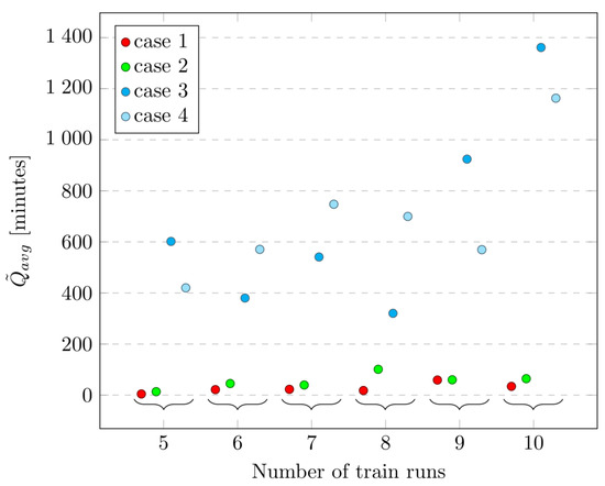
Figure 4. Dependence of ${\tilde{Q}}_{avg}$ (minutes) on the number of train runs for selected cases.

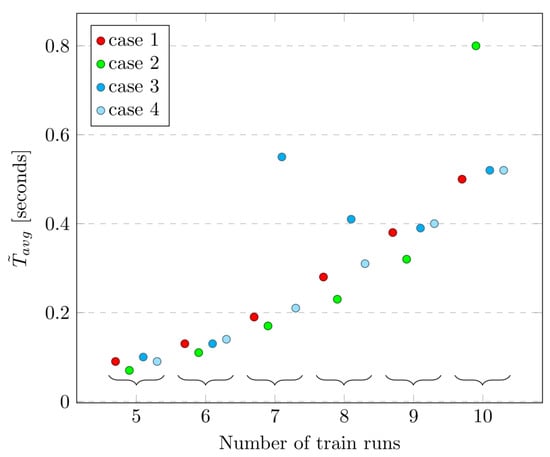
Figure 5. Dependence of ${\tilde{T}}_{avg}$ (seconds) on the number of train runs for selected cases.

As can be seen in Figure 5 and Table 7, computational time of Algorithm 4 grows in a nearly linear manner concerning the number of runs. This property is crucial to the computational time of the heuristic algorithm, which uses Algorithm 3 repeatedly and for sub-problems of varying sizes. We notice from Figure 4 and Table 6 that $\tilde{Q}$ varies significantly, with much greater values obtained for longer expected train movement times. This remark gives a clear message that it is easier to permit closures on the tracks for fast passenger trains. Slow trains will likely have to change their route or be canceled. Comparison with optimal solutions leads to a natural conclusion that the Algorithm 4 provides similar results for the majority of all the tested cases. As it can be apparently seen from Table 6, all of the results obtained by the algorithm were optimal for Cases 1 and 2. For Cases 3 and 4, the algorithm failed to find a solution in 5% of the experiments even though one existed. The overall difference in quality between the solution provided by Algorithm 4 and the optimal solution was under 1% of the latter. The cause of those minor differences lies in potential sub-optimality of the orderings obtained with the use of greedy Algorithms 6 and 7.

From the experiments, it is clear that increasing duration of train movement between stations decreases the efficiency of Algorithm 4. Nevertheless, for the majority of tested cases, the difference between Algorithm 4 and the optimal solution is slight.

6.2. Single Track Timetable

Let us consider a single track case as in the previous section for closure with the following parameters $T_0^{\mathrm{C}}=50,t_0^{\mathrm{CES}}=0,t_0^{\mathrm{CLS}}=105,R_{0,1,2,1}^{\mathrm{C}}$, and four trains with timetable as follows:

• Run $p=0$ station visit order: $0,1,2,0$, arrival and departure times $t_{0,0}^{\mathrm{DEP}}=t_{1,0}^{\mathrm{ARR}}=0,t_{1,1}^{\mathrm{DEP}}=5,t_{2,0}^{\mathrm{ARR}}=55,t_{2,0}^{\mathrm{DEP}}=t_{0,0}^{\mathrm{ARR}}=60,t_{2,0}^{\mathrm{ARR}}\le 300$.
• Run $p=1$ station visit order: $0,1,2,0$, arrival and departure times $t_{0,1}^{\mathrm{DEP}}=t_{1,1}^{\mathrm{ARR}}=50,t_{1,1}^{\mathrm{DEP}}=55,t_{2,1}^{\mathrm{ARR}}=105,t_{2,1}^{\mathrm{DEP}}=t_{0,1}^{\mathrm{ARR}}=110,t_{2,1}^{\mathrm{ARR}}\le 300$.
• Run $p=2$ station visit order: $0,1,2,0$, arrival and departure times $t_{0,2}^{\mathrm{DEP}}=t_{1,1}^{\mathrm{ARR}}=50,t_{1,2}^{\mathrm{DEP}}=105,t_{2,2}^{\mathrm{ARR}}=155,t_{2,2}^{\mathrm{DEP}}=t_{0,2}^{\mathrm{ARR}}=160,t_{2,2}^{\mathrm{ARR}}\le 300$.
• Run $p=3$ station visit order: $0,2,1,0$, arrival and departure times $t_{0,3}^{\mathrm{DEP}}=t_{2,3}^{\mathrm{ARR}}=155,t_{2,3}^{\mathrm{DEP}}=160,t_{1,3}^{\mathrm{ARR}}=210,t_{1,3}^{\mathrm{DEP}}=t_{0,3}^{\mathrm{ARR}}=215,t_{2,3}^{\mathrm{ARR}}\le 300$.

The timetables of train runs before and after the closure are in Figure 6 and Figure 7. The figures represent the connection between the time and the distance traveled between nodes (stations) 1 and 2 for different trains. Red represents the time of the closure.

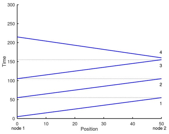
Figure 6. Timetable before closures.

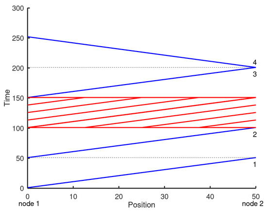
Figure 7. Timetable after closures.

6.3. Network of Tracks Case

The second part of experiments was performed on a multi-station network. The considered network is based on the part of the Polish Railway Network from the region of Kielce consisting of 167 tracks connecting 149 stations as it is depicted in Figure 8, and there were originally 95 train runs in the official timetable for one day. The simulations have been performed for different numbers of train runs $TR$ (i.e., for $TR=10,11,12,13,14,15,20,30$) using the same railway network. Ten different sub-sets of the original set of train runs selected at random according to the uniform probability distribution have been generated for a given number of train runs. Each train run was assumed as obligatory. The standing times have been set to $T^{\mathrm{DL}}=15$, $T_{i,p}^{\mathrm{D}}=1$ for all runs p and stations i. We also assumed that there were three closures in the railway network. Each closure was also assumed as obligatory. Unless otherwise stated, the closures’ duration times have been set to 2h (i.e., $T_n^{\mathrm{C}}=2h$ for all n). For each simulation, the closures’ tracks have been randomly chosen according to the uniform distribution and the closures’ beginning times have also been chosen analogously from the interval $(0,T^{\mathrm{H}}-2h)$. These assumptions correspond to the periodic and weekly closure planning when short-term closures caused by the regular maintenance works are taken into consideration. We have limited our consideration to the determination of the plan for one day assuming that the train runs timetable and the closures plan should be repeatable. There stations’ capacities have been unlimited. As for a single track case, the overall time interval was also limited to a single day, i.e., $T^{\mathrm{H}}=1440$ min. The results are briefly presented in Figure 9, Figure 10, Figure 11 and Figure 12 and in corresponding Table 8, Table 9, Table 10 and Table 11. Dots, as well as error bars, represent the average value, as well as minimal and maximal values, respectively. The dimensionless performance index $\widehat{Q}=\frac{Q}{\tilde{Q}}$, where $\tilde{Q}$ stands for the best value of (17) found for the particular problem instance along with the computation time $\tilde{T}$, evaluates the heuristic algorithm. Analogously as in Section 6.1, we denote the average, minimum, and maximum values of $\widehat{Q}$ by ${\widehat{Q}}_{avg}$, ${\widehat{Q}}_{min}$, ${\widehat{Q}}_{max}$, respectively.

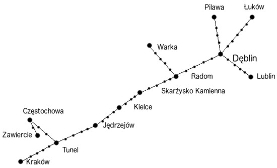
Figure 8. The considered part of the Polish Railway Network in the area of Kielce (only selected main stations are indicated by dots).

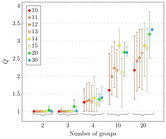
Figure 9. Dependence of $\widehat{Q}$ on the number of groups for selected numbers of train runs.

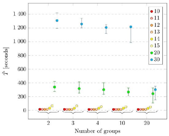
Figure 10. Dependence of $\tilde{T}$ (seconds) on the number of groups for selected numbers of train runs.

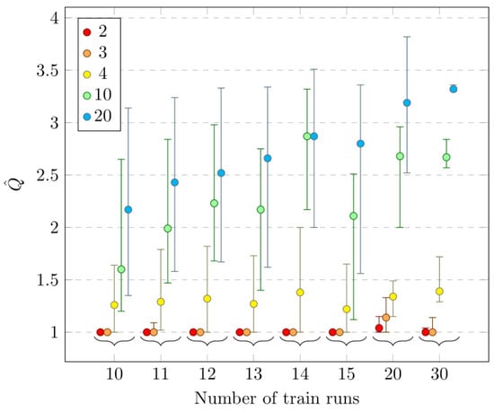
Figure 11. Dependence of $\widehat{Q}$ on the number of train runs for selected numbers of groups.

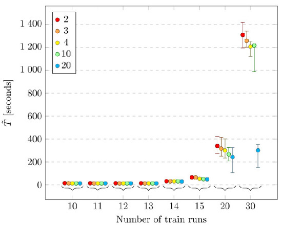
Figure 12. Dependence of $\tilde{T}$ (seconds) on the number of train runs for selected numbers of groups.

Table 8. Dependence of $\widehat{Q}$ on $\eta$ for different $TR$.

$\mathit{\eta }$	$\mathit{TR}=10$			$\mathit{TR}=11$			$\mathit{TR}=12$			$\mathit{TR}=13$
	${\widehat{\mathit{Q}}}_{\mathit{avg}}$	${\widehat{\mathit{Q}}}_{\mathit{min}}$	${\widehat{\mathit{Q}}}_{\mathit{max}}$	${\widehat{\mathit{Q}}}_{\mathit{avg}}$	${\widehat{\mathit{Q}}}_{\mathit{min}}$	${\widehat{\mathit{Q}}}_{\mathit{max}}$	${\widehat{\mathit{Q}}}_{\mathit{avg}}$	${\widehat{\mathit{Q}}}_{\mathit{min}}$	${\widehat{\mathit{Q}}}_{\mathit{max}}$	${\widehat{\mathit{Q}}}_{\mathit{avg}}$	${\widehat{\mathit{Q}}}_{\mathit{min}}$	${\widehat{\mathit{Q}}}_{\mathit{max}}$
2	1	1	1	1	1	1	1	1	1	1	1	1
3	1	1	1	1	1	1.09	1	1	1	1	1	1
4	1.26	1	1.64	1.29	1.02	1.79	1.32	1	1.82	1.27	1	1.73
10	1.6	1.2	2.65	1.99	1.47	2.84	2.23	1.68	2.98	2.17	1.4	2.75
20	2.17	1.35	3.14	2.43	1.58	3.24	2.52	1.67	3.33	2.66	1.62	3.34
$\mathit{\eta }$	$\mathit{TR}=\mathbf{14}$			$\mathit{TR}=\mathbf{15}$			$\mathit{TR}=\mathbf{20}$			$\mathit{TR}=\mathbf{30}$
	${\widehat{\mathit{Q}}}_{\mathit{avg}}$	${\widehat{\mathit{Q}}}_{\mathit{min}}$	${\widehat{\mathit{Q}}}_{\mathit{max}}$	${\widehat{\mathit{Q}}}_{\mathit{avg}}$	${\widehat{\mathit{Q}}}_{\mathit{min}}$	${\widehat{\mathit{Q}}}_{\mathit{max}}$	${\widehat{\mathit{Q}}}_{\mathit{avg}}$	${\widehat{\mathit{Q}}}_{\mathit{min}}$	${\widehat{\mathit{Q}}}_{\mathit{max}}$	${\widehat{\mathit{Q}}}_{\mathit{avg}}$	${\widehat{\mathit{Q}}}_{\mathit{min}}$	${\widehat{\mathit{Q}}}_{\mathit{max}}$
2	1	1	1	1	1	1	1.04	1	1.15	1	1	1.04
3	1	1	1	1	1	1	1.14	1	1.33	1.01	1	1.14
4	1.38	1	2	1.22	1	1.65	1.34	1.15	1.49	1.39	1.29	1.72
10	2.87	2.17	3.32	2.11	1.12	2.51	2.68	2	2.96	2.67	2.57	2.84
20	2.87	2	3.51	2.8	1.56	3.36	3.19	2.52	3.82	3.32	3.3	3.36

Table 9. Dependence of $\tilde{T}$ on $\eta$ for different $TR$.

$\mathit{\eta }$	$\mathit{TR}=10$			$\mathit{TR}=11$			$\mathit{TR}=12$			$\mathit{TR}=13$
	${\tilde{\mathit{T}}}_{\mathit{avg}}$	${\tilde{\mathit{T}}}_{\mathit{min}}$	${\tilde{\mathit{T}}}_{\mathit{max}}$	${\tilde{\mathit{T}}}_{\mathit{avg}}$	${\tilde{\mathit{T}}}_{\mathit{min}}$	${\tilde{\mathit{T}}}_{\mathit{max}}$	${\tilde{\mathit{T}}}_{\mathit{avg}}$	${\tilde{\mathit{T}}}_{\mathit{min}}$	${\tilde{\mathit{T}}}_{\mathit{max}}$	${\tilde{\mathit{T}}}_{\mathit{avg}}$	${\tilde{\mathit{T}}}_{\mathit{min}}$	${\tilde{\mathit{T}}}_{\mathit{max}}$
2	15	14	16	14	14	14	14	14	14	14	14	14
3	14	13	15	13	13	13	13	13	13	13	13	13
4	13	13	14	13	13	13	13	13	13	13	13	13
10	13	13	14	13	13	13	13	13	13	13	13	13
20	13	13	14	13	13	13	13	13	13	13	13	13
$\mathit{\eta }$	$\mathit{TR}=\mathbf{14}$			$\mathit{TR}=\mathbf{15}$			$\mathit{TR}=\mathbf{20}$			$\mathit{TR}=\mathbf{30}$
	${\tilde{\mathit{T}}}_{\mathit{avg}}$	${\tilde{\mathit{T}}}_{\mathit{min}}$	${\tilde{\mathit{T}}}_{\mathit{max}}$	${\tilde{\mathit{T}}}_{\mathit{avg}}$	${\tilde{\mathit{T}}}_{\mathit{min}}$	${\tilde{\mathit{T}}}_{\mathit{max}}$	${\tilde{\mathit{T}}}_{\mathit{avg}}$	${\tilde{\mathit{T}}}_{\mathit{min}}$	${\tilde{\mathit{T}}}_{\mathit{max}}$	${\tilde{\mathit{T}}}_{\mathit{avg}}$	${\tilde{\mathit{T}}}_{\mathit{min}}$	${\tilde{\mathit{T}}}_{\mathit{max}}$
2	32	30	35	65	60	67	339	275	421	1308	1193	1419
3	31	29	36	64	61	67	316	251	415	1257	1201	1341
4	31	29	34	53	59	63	300	234	401	1206	1119	1250
10	31	28	33	50	46	61	267	210	326	1216	987	1233
20	29	28	31	48	39	58	242	107	326	301	151	351

Table 10. Dependence of $\widehat{Q}$ on $TR$ for different $\eta$.

$\mathit{TR}$	$\mathit{\eta }=2$			$\mathit{\eta }=3$			$\mathit{\eta }=4$			$\mathit{\eta }=10$			$\mathit{\eta }=20$
	${\widehat{\mathit{Q}}}_{\mathit{avg}}$	${\widehat{\mathit{Q}}}_{\mathit{min}}$	${\widehat{\mathit{Q}}}_{\mathit{max}}$	${\widehat{\mathit{Q}}}_{\mathit{avg}}$	${\widehat{\mathit{Q}}}_{\mathit{min}}$	${\widehat{\mathit{Q}}}_{\mathit{max}}$	${\widehat{\mathit{Q}}}_{\mathit{avg}}$	${\widehat{\mathit{Q}}}_{\mathit{min}}$	${\widehat{\mathit{Q}}}_{\mathit{max}}$	${\widehat{\mathit{Q}}}_{\mathit{avg}}$	${\widehat{\mathit{Q}}}_{\mathit{min}}$	${\widehat{\mathit{Q}}}_{\mathit{max}}$	${\widehat{\mathit{Q}}}_{\mathit{avg}}$	${\widehat{\mathit{Q}}}_{\mathit{min}}$	${\widehat{\mathit{Q}}}_{\mathit{max}}$
10	1	1	1	1	1	1	1.26	1	1.64	1.6	1.2	2.65	2.17	1.35	3.14
11	1	1	1	1	1	1.09	1.29	1.02	1.79	1.99	1.47	2.84	2.43	1.58	3.24
12	1	1	1	1	1	1	1.32	1	1.82	2.23	1.68	2.98	2.52	1.67	3.33
13	1	1	1	1	1	1	1.27	1	1.73	2.17	1.4	2.75	2.66	1.62	3.34
14	1	1	1	1	1	1	1.38	1	2	2.87	2.17	3.32	2.87	2	3.51
15	1	1	1	1	1	1	1.22	1	1.65	2.11	1.12	2.51	2.8	1.56	3.36
20	1.04	1	1.15	1.14	1	1.33	1.34	1.15	1.49	2.68	2	2.96	3.19	2.52	3.82
30	1	1	1.04	1.01	1	1.14	1.39	1.29	1.72	2.67	2.57	2.84	3.32	3.3	3.36

Table 11. Dependence of $\tilde{T}$ on $TR$ for different $\eta$.

$\mathit{TR}$	$\mathit{\eta }=2$			$\mathit{\eta }=3$			$\mathit{\eta }=4$			$\mathit{\eta }=10$			$\mathit{\eta }=20$
	${\tilde{\mathit{T}}}_{\mathit{avg}}$	${\tilde{\mathit{T}}}_{\mathit{min}}$	${\tilde{\mathit{T}}}_{\mathit{max}}$	${\tilde{\mathit{T}}}_{\mathit{a}\mathit{v}\mathit{g}}$	${\tilde{\mathit{T}}}_{\mathit{min}}$	${\tilde{\mathit{T}}}_{\mathit{max}}$	${\tilde{\mathit{T}}}_{\mathit{avg}}$	${\tilde{\mathit{T}}}_{\mathit{min}}$	${\tilde{\mathit{T}}}_{\mathit{max}}$	${\tilde{\mathit{T}}}_{\mathit{avg}}$	${\tilde{\mathit{T}}}_{\mathit{min}}$	${\tilde{\mathit{T}}}_{\mathit{max}}$	${\tilde{\mathit{T}}}_{\mathit{avg}}$	${\tilde{\mathit{T}}}_{\mathit{min}}$	${\tilde{\mathit{T}}}_{\mathit{max}}$
10	15	14	16	14	13	15	13	13	14	13	13	14	13	13	14
11	14	14	14	13	13	13	13	13	13	13	13	13	13	13	13
12	14	14	14	13	13	13	13	13	13	13	13	13	13	13	13
13	14	14	14	13	13	13	13	13	13	13	13	13	13	13	13
14	32	30	35	31	29	36	31	29	34	31	28	33	29	28	31
15	65	60	67	64	61	67	53	59	63	50	46	61	48	39	58
20	339	275	421	316	251	415	300	234	401	267	210	326	242	107	326
30	1308	1193	1419	1257	1201	1341	1206	1119	1250	1216	987	1233	301	151	351

We can observe in Figure 9 and Figure 11 that the growing number of groups $\eta$ has the significant influence on the deterioration of solution quality, and it does not improve much the computation time (Figure 10 and Figure 12), i.e., the computation time for a fixed number of train runs does not decrease significantly with increasing number of groups. The increase in the number of groups from 2 to 20 deteriorates the quality of solution up to 320%, with only about 26% saving of the computational time. However, when the aim is to check fast the existence of any feasible solution, and the quality of the solution is meaningless, the decomposition into smaller groups may be justified.

The growth of the number of groups (railway sub-networks) $\eta$ deteriorates the obtained solutions for the same number of train runs $TR$ (Figure 13 and Table 12). A similar situation occurs when the number of train runs $TR$ grows for the fixed number of groups $\eta$ (Figure 14 and Table 13). Nevertheless, the worsening is less significant in the latter case.

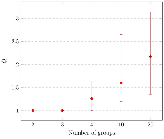
Figure 13. Dependence of $\widehat{Q}$ on the number of groups for 10 train runs.

Table 12. Dependence of $\widehat{Q}$ on $\eta$ for different $TR=10$.

$\mathit{\eta }$	${\widehat{\mathit{Q}}}_{\mathit{avg}}$	${\widehat{\mathit{Q}}}_{\mathit{min}}$	${\widehat{\mathit{Q}}}_{\mathit{max}}$
2	1	1	1
3	1	1	1
4	1.64	1	1.26
10	2.65	1.2	1.6
20	3.14	1.35	2.17

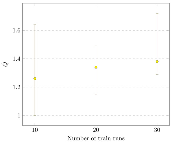
Figure 14. Dependence of $\widehat{Q}$ on the number of train runs for 4 groups.

Table 13. Dependence of $\widehat{Q}$ on $TR$ for different $\eta =4$.

$\mathit{TR}$	${\widehat{\mathit{Q}}}_{\mathit{avg}}$	${\widehat{\mathit{Q}}}_{\mathit{min}}$	${\widehat{\mathit{Q}}}_{\mathit{max}}$
10	1.64	1	1.26
20	1.49	1.15	1.34
30	1.72	1.29	1.38

The performance indexes $\widehat{Q}$ values are jointly compared with the computational time $\tilde{T}$ in Figure 15 and Table 14, while the performance index $\tilde{Q}$ are jointly compared with the computational time $\tilde{T}$ in Figure 16 and Table 15. The values of $\widehat{Q}$ are marked on the abscissa axis, and $\tilde{Q}$ values are represented by dots, in Figure 15. The opposite presentation is used in Figure 16, where values of $\tilde{Q}$ are represented on the logarithmic abscissa axis, while $\widehat{Q}$ are marked by dots. Both figures present the comparison for different values of $TR$ and $\eta$. As it can be observed there, the impact of the number of groups $\eta$ on the computation time is slight, unlike the solution quality $\tilde{Q}$. So, it is not recommended to decompose the problem into many sub-problems, as it deteriorates inadmissibly the quality.

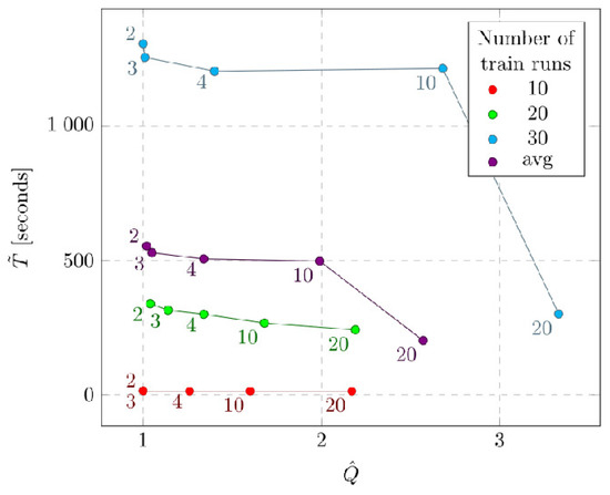
Figure 15. Relation between $\widehat{Q}$ and $\tilde{T}$ (seconds) for selected numbers of train runs and groups (at stations).

Table 14. Dependence of $\widehat{Q}$ and $\tilde{T}$ for selected $TR$ and $\eta$.

$\mathit{\eta }$	$\mathit{TR}=10$		$\mathit{TR}=20$		$\mathit{TR}=30$		$\mathit{avg}$
	${\widehat{\mathit{Q}}}_{\mathit{avg}}$	${\tilde{\mathit{T}}}_{\mathit{avg}}$	${\widehat{\mathit{Q}}}_{\mathit{avg}}$	${\tilde{\mathit{T}}}_{\mathit{avg}}$	${\widehat{\mathit{Q}}}_{\mathit{avg}}$	${\tilde{\mathit{T}}}_{\mathit{avg}}$	${\widehat{\mathit{Q}}}_{\mathit{avg}}$	${\tilde{\mathit{T}}}_{\mathit{avg}}$
2	1	15	1.05	339	1	1308	1.02	554
3	1	14	1.15	315	1.01	1257	1.05	529
4	1.27	13	1.34	300	1.4	1206	1.34	506
10	1.6	13	1.69	267	2.68	1216	1.99	499
20	2.17	13	2.2	242	3.33	301	2.56	202

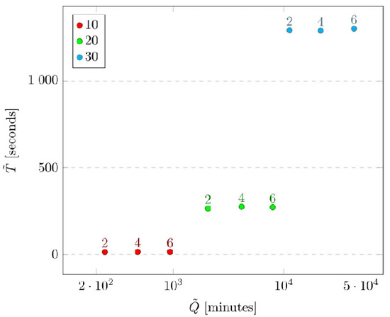
Figure 16. Relation between $\widehat{Q}$ and $\tilde{T}$ (seconds) for selected closure durations for 10, 20, 30 train runs and for 3 groups.

Table 15. Dependence of Q and $\tilde{T}$ for $T_n\in \{2,4,6\}$, $TR\in \{10,20,30\}$, and $\eta =3$.

${\mathit{T}}_{\mathit{n}}$	$\mathit{TR}=10$		$\mathit{TR}=20$		$\mathit{TR}=30$
	${\mathit{Q}}_{\mathit{avg}}$	${\tilde{\mathit{T}}}_{\mathit{avg}}$	${\mathit{Q}}_{\mathit{avg}}$	${\tilde{\mathit{T}}}_{\mathit{avg}}$	${\mathit{Q}}_{\mathit{avg}}$	${\tilde{\mathit{T}}}_{\mathit{avg}}$
2	239	13	2052	264	11231	1292
4	474	14	4123	274	21452	1290
6	931	14	7905	271	43041	1301

However, it is worth noting that the main challenge consists of answering the question if there is any feasible solution, and it is necessary to obtain the answer in the limited time. So, the most important issue is to obtain any solution in such time. On the other hand, the decision-maker has to be aware that the decreasing of computational time by applying bigger values of $\eta$ can result in the lack of any solution. Even though the feasible solution of the considered problem may exist, the algorithm can fail to find it. Such a situation can be observed in Table 16, where the algorithm for $\eta \ge 20$ did not find any solution in 20% of all examined cases.

Table 16. Number of cases with feasible solutions found for selected $TR$ and $\eta$.

$\mathit{TR}$	$\mathit{\eta }=2$	$\mathit{\eta }=3$	$\mathit{\eta }=4$	$\mathit{\eta }=10$	$\mathit{\eta }=20$	$\mathit{\eta }=25$
10	10	10	10	10	10	10
20	10	10	10	10	10	10
30	10	10	10	10	8	8

7. Final Remarks

The selected management problem on railway transportation under anticipated track closures is considered. Taking into account the planned closures, caused mainly by the maintenance of tracks and stations, requires the elaboration of a new timetable for trains. In consequence, the problems of track closure planning and train rescheduling are jointly considered in the paper as the strongly multivariable and nonlinear mixed integer optimization problem. A novel approach based on the decomposition is applied, which results in the heuristic solution algorithm. The conducted simulation experiments confirmed the usefulness of the algorithm regarding both the performance index applied and the computational time. In particular, the experiments performed on single tracks have shown that the results generated by the heuristic algorithm are quite close to the optimal ones. Such experiments involving optimal solutions are impossible for greater instances of the problem. Hence, the profound simulation experiments were performed for the real-world example including 95 train runs. The results confirmed the effectiveness of the algorithm for a wide range of the algorithm’s parameters, first of all for the different number of groups (railway sub-networks) being the result of the applied decomposition. The computational time did not exceed a half an hour for the real-world instance considered. So, it is possible to effectively launch the algorithm for substantially big problem instances. The proposed solution algorithm with the number of railway sub-networks $\eta$ as the algorithm’s parameter also allows for fast checking of the existence of any feasible solution neglecting the optimization of the criterion. Such property of the algorithm seems to be very important for real-world applications.

The verification of the current model is now considered for the case when a substitutive transport with resulted additional costs is possible. Planned further works will consist mainly of the generalization of the model proposed in Section 3, by taking into account additional facets important for railway networks management as different categories of trains and priorities in their running, as well as additional constraints on station capacities and track forks.

References

- Arenas, D.; Chevrier, R.; Rodriguez, J.; Dhaenens, C.; Hanafi, S. Application of a co-evolutionary genetic algorithm to solve the periodic railway timetabling problem. In Proceedings of the 2013 IEEE International Conference on Industrial Engineering and Systems Management (IESM), Agdal, Morocco, 28–30 October 2013. [Google Scholar]
- Goverde, R.M.; Besinovic, N.; Binder, A.; Cacchiani, V.; Quaglietta, E.; Roberti, R.; Toth, P. A three-level framework for performance-based railway timetabling. In Proceedings of the 6th International conference on Railway Operations Modelling and Analysis, RailTokyo 2015, Narashimo, Japan, 23–26 March 2015. [Google Scholar]
- Niu, H.; Zhou, X. Optimizing urban rail timetable under time-dependent demand and oversaturated conditions. Transp. Res. Part C Emerg. Technol. 2013, 36, 212–230. [Google Scholar] [CrossRef]
- Barrena, E.; Canca, D.; Coelho, L.C.; Laporte, G. Exact formulations and algorithm for the train timetabling problem with dynamic demand. Comput. Oper. Res. 2014, 44, 66–74. [Google Scholar] [CrossRef]
- Filcek, G.; Gąsior, D.; Hojda, M.; Józefczyk, J. Joint Train Rescheduling and Track Closures Planning: Model and Solution Algorithm. In Information Systems Architecture and Technology: Proceedings of 36th International Conference on Information Systems Architecture and Technology—ISAT 2015–Part I; Springer International Publishing: Berlin/Heidelberg, Germany, 2016; pp. 215–225. [Google Scholar]
- Hojda, M.; Filcek, G. A Joint Problem of Track Closure Planning and Train Run Rescheduling with Detours. In Advances in Intelligent Systems and Computing—Advances in Systems Science 539; Springer International Publishing: Berlin/Heidelberg, Germany, 2017; pp. 285–294. [Google Scholar]
- Bach, L.; Dollevoet, T.; Huisman, D. Integrating timetabling and crew scheduling at a freight railway operator. Transp. Sci. 2016, 50, 878–891. [Google Scholar] [CrossRef]
- Zhang, Y.; D’Ariano, A.; He, B.; Peng, Q. Microscopic optimization model and algorithm for integrating train timetabling and track maintenance task scheduling. Transp. Res. Part B Methodol. 2019, 127, 237–278. [Google Scholar] [CrossRef]
- Zhang, C.; Gao, Y.; Yang, L.; Gao, Z.; Qi, J. Joint optimization of train scheduling and maintenance planning in a railway network: A heuristic algorithm using Lagrangian relaxation. Transp. Res. Part B Methodol. 2020, 134, 64–92. [Google Scholar] [CrossRef]
- Corman, F.; Meng, L. A Review of Online Dynamic Models and Algorithms for Railway Traffic Management. IEEE Trans. Intell. Transp. Syst. 2015, 16, 1274–1284. [Google Scholar] [CrossRef]
- Schobel, A. A model for the delay management problem based on Mixed Integer Programming. Electron. Notes Theor. Comput. Sci. 2001, 50, 1–10. [Google Scholar] [CrossRef]
- Schobel, A. Capacity constraints in delay management. J. Public Transp. 2009, 1, 135–154. [Google Scholar] [CrossRef]
- Brännlund, U.; Lindberg, P.O.; Nõu, A.; Nilsson, J.-E. Railway timetabling using Lagrangian relaxation. Transp. Sci. 1998, 32, 358–369. [Google Scholar] [CrossRef]
- Petersen, E.; Taylor, A. Line block prevention in rail line dispatch and simulation models. Inf. Syst. Oper. Res. 1983, 21, 46–51. [Google Scholar] [CrossRef]
- Ping, L.; Axin, N.; Limin, J.; Fuzhang, W. Study on intelligent train dispatching. In Proceedings of the IEEE Intelligent Transportation Systems Conference Proceedings, Oakland, CA, USA, 25–29 August 2001. [Google Scholar]
- Zhang, Z.; Zhu, C.; Ma, W. Discrete Optimization on Train Rescheduling on Single-Track Railway: Clustering Hierarchy and Heuristic Search. J. Adv. Transp. 2020, 2020. [Google Scholar] [CrossRef]
- Tornquist, J.; Persson, J. N-tracked railway traffic rescheduling during disturbances. Transp. Res. Part B 2007, 41, 342–362. [Google Scholar] [CrossRef]
- Dessouky, M.M.; Lu, Q.; Zhao, J.; Leachman, R.C. An exact solution procedure to determine the optimal dispatching times for complex rail networks. IIE Trans. 2006, 38, 141–152. [Google Scholar] [CrossRef]
- Acuna-Agost, R.; Michelon, P.; Feillet, D.; Guaye, S. Constraint Programming and Mixed Integer Linear Programming for Rescheduling Trains under Disrupted Operations A Comparative Analysis of Models, Solution Methods, and Their Integration. Springer Lect. Notes Comput. Sci. 2009, 5547/2009, 312–313. [Google Scholar]
- Cacchiani, V.; Huisman, D.; Kidd, M.; Kroon, L.; Toth, P.; Veelentruf, L.; Wagenaar, J. An overview of recovery models and algorithms for real-time railway rescheduling. Transp. Res. Part B Methodol. 2014, 63, 15–37. [Google Scholar] [CrossRef]
- Mascis, A.; Pacciarelli, D. Job shop scheduling with blocking and no-wait constraints. Eur. J. Oper. Res. 2002, 143, 498–517. [Google Scholar] [CrossRef]
- Sama, M.; Pellegrini, P.; D’Ariano, A.; Rodriguez, J.; Pacciarelli, D. The potential of the routing selection problem in real-time railway traffic management. In Proceedings of the 7th International Conference on Railway Operations Modelling and Analysis, Lille, France, 4–7 April 2017. [Google Scholar]
- Harrod, S. Modeling network transition constraints with hypergraphs. Transp. Sci. 2011, 45, 81–97. [Google Scholar] [CrossRef]
- He, B.; Song, R.; He, S.; Xu, Y. High-Speed Rail Train Timetabling Problem: A Time-Space Network Based Method with an Improved Branch-and-Price Algorithm. Math. Probl. Eng. 2014, 2014, 15. [Google Scholar] [CrossRef]
- Acuna-Agost, R. Mathematical Modeling and Methods for Rescheduling Trains under Disrupted Operations; Universitéd’Avignon et des Pays de Vaucluse: Avignon, France, 2010. [Google Scholar]
- Tornquist, J.; Persson, J.A. Train traffic deviation handling using Tabu Search and Simulated Annealing. In Proceedings of the 38th Hawaii International Conference on System Sciences (HICSS38), Big Island, HI, USA, 3–6 January 2005. [Google Scholar]
- Veelenturf, L.P.; Kidd, M.P.; Cacchiani, V.; Kroon, L.G.; Toth, P. A railway timetable rescheduling approach for handling large-scale disruptions. Transp. Sci. 2015, 50, 841–862. [Google Scholar] [CrossRef]
- Andersson, E.; Peterson, A.; Törnquist Krasemann, J. Improved Railway Timetable Robustness for Reduced Traffic Delays–a MILP approach. In Proceedings of the 6th International conference on Railway Operations Modelling and Analysis, RailTokyo 2015, Narashimo, Japan, 23–26 March 2015. [Google Scholar]
- Heydar, M.; Petering, M.E.; Bergmann, D.R. Mixed integer programming for minimizing the period of a cyclic railway timetable for a single track with two train types. Comput. Ind. Eng. 2013, 66, 171–185. [Google Scholar] [CrossRef]
- Louwerse, I.; Huisman, D. Adjusting a railway timetable in case of partial or complete blockades. Eur. J. Oper. Res. 2014, 235, 583–593. [Google Scholar] [CrossRef]
- Wang, Y.; Wei, Y.; Zhang, Q.; Shi, H.; Pang, P. Scheduling overnight trains for improving both last and first train services in an urban subway network. Adv. Mech. Eng. 2019, 11, 1–19. [Google Scholar] [CrossRef]
- Altazin, E.; Dauzère-Pérès, S.; Ramond, F.; Tréfond, S. A multi-objective optimization-simulation approach for real time rescheduling in dense railway systems. Eur. J. Oper. Res. 2020, 286, 662–672. [Google Scholar] [CrossRef]
- Zhong, Q.; Zhang, Y.; Wang, D.; Zhong, Q.; Wen, C.; Peng, Q. A Mixed Integer Linear Programming Model for Rolling Stock Deadhead Routing before the Operation Period in an Urban Rail Transit Line. J. Adv. Transp. 2020, 1–18. [Google Scholar] [CrossRef]
- Dekker, R. Applications of maintenance optimization models: A review and analysis. Reliab. Eng. Syst. Saf. 1996, 51, 229–240. [Google Scholar] [CrossRef]
- Higgins, A.; Ferreira, L.; Lake, M. Scheduling rail track maintenance to minimise overall delays. In Proceedings of the 14th International Symposium on Transportation and Traffic Theory, Jerusalem, Israel, 20–23 July 1999. [Google Scholar]
- Budai, G.; Huisman, D.; Dekker, R. Scheduling preventive railway main- tenance activities. J. Oper. Res. Soc. 2006, 57, 1035–1044. [Google Scholar] [CrossRef]
- Higgins, A. Scheduling of railway track maintenance activities and crews. J. Oper. Res. Soc. 1998, 49, 1026–1033. [Google Scholar] [CrossRef]
- Khalouli, S.; Benmansour, R.; Hanafi, S. An ant colony algorithm based on opportunities for scheduling the preventive railway maintenance. In Proceedings of the Control, Decision and Information Technologies (CoDIT), Saint Julian’s, Malta, 6–8 April 2016. [Google Scholar]
- Lidén, T.; Joborn, M. Dimensioning windows for railway infrastructure maintenance: Cost efficiency versus traffic impact. J. Rail Transp. Plan. Manag. 2016, 6, 32–47. [Google Scholar] [CrossRef]
- Lidén, T. Railway infrastructure maintenance-a survey of planning problems and conducted research. Transp. Res. Procedia 2015, 10, 574–583. [Google Scholar] [CrossRef]
- Lidén, T. Survey of Railway Maintenance Activities from a Planning Perspective and Literature Review Concerning the Use of Mathematical Algorithms for Solving Such Planning and Scheduling Problems; Technical Report; Department of Science and Technology, Linköping University: Linköping, Sweden, 2014. [Google Scholar]
- Kiefer, A.; Schilde, M.; Doerner, K. Scheduling of maintenance work of a large-scale tramway network. Eur. J. Oper. Res. 2018, 270, 1158–1170. [Google Scholar] [CrossRef]
- Jovanovic, D.; Harker, P.T. Tactical scheduling of rail operations: The SCAN I system. Transp. Sci. 1991, 25, 46–64. [Google Scholar] [CrossRef]
- Kraay, D.R.; Harker, P.T. Real-time scheduling of freight railroads. Transp. Res. Part B 1995, 29, 213–229. [Google Scholar] [CrossRef]
- Van Zante-de Fokkert, J.I.; den Hertog, D.; van den Berg, F.J.; Verhoeven, J.H.M. The Netherlands schedules track maintenance to improve track workers’ safety. Interfaces 2007, 37, 133–142. [Google Scholar] [CrossRef]
- Albrecht, A.R.; Panton, D.M.; Lee, D.H. Rescheduling rail networks with maintenance disruptions using problem space search. Comput. Oper. Res. 2013, 40, 703–712. [Google Scholar] [CrossRef]
- Albrecht, A. Integrating Railway Track Maintenance and Train Timetables. Ph.D. Thesis, University of South Australia, Adelaide, Australia, 2009. [Google Scholar]
- Forsgren, M.; Aronsson, M.; and Gestrelius, S. Maintaining tracks and traffic flow at the same time. J. Rail Transp. Plan. Manag. 2013, 3, 111–123. [Google Scholar] [CrossRef]
- Lidén, T.; Joborn, M. An optimization model for integrated planning of railway traffic and network maintenance. Transp. Res. Part C Emerg. Technol. 2017, 74, 327–347. [Google Scholar] [CrossRef]
- Lidén, T. Reformulations for Integrated Planning of Railway Traffic and Network Maintenance. In Proceedings of the 18th Workshop on Algorithmic Approaches for Transp. Modelling, Optimization, and Systems, Helsinki, Finland, 23–24 August 2018; Borndörfer, R., Storandt, S., Eds.; Schloss Dagstuhl–Leibniz-Zentrum fuer Informatik: Dagstuhl, Germany, 2018; pp. 1:1–1:10. [Google Scholar]
- Lidén, T.; Kalinowski, T.; Waterer, H. Resource considerations for integrated planning of railway traffic and maintenance windows. J. Rail Transp. Plan. Manag. 2018, 8, 1–15. [Google Scholar] [CrossRef]
- Luan, X.; Miao, J.; Meng, L.; Corman, F.; Lodewijks, G. Integrated optimization on train scheduling and preventive maintenance time slots planning. Transp. Res. Part C Emerg. Technol. 2017, 80, 329–359. [Google Scholar] [CrossRef]
- Aken, S.V.; Bešinović, N.; Goverde, R.M.P. Designing alternative railway timetables under infrastructure maintenance possessions. Transp. Res. Part B Methodol 2017, 98, 224–238. [Google Scholar] [CrossRef]
- Arenas, D.; Pellegrini, P.; Hanafi, S.; Rodriguez, J. Timetable rearrangement to cope with railway maintenance activities. Comput. Oper. Res. 2018, 95, 123–138. [Google Scholar] [CrossRef]
- Zhang, C.; Gao, Y.; Yang, L.; Kumar, U.; Gao, Z. Integrated optimization of train scheduling and maintenance planning on high-speed railway corridors. Omega 2019, 87, 86–104. [Google Scholar] [CrossRef]
- Cavone, G.; Blenkers, T.; van den Boom, T.; Dotoli, M.; Seatzu, C.; De Schutter, B. Railway disruption: A bi-level rescheduling algorithm. In Proceedings of the 6th International Conference on Control, Decision and Information Technologies (CoDIT’19), Paris, France, 23–26 April 2019; pp. 54–59. [Google Scholar]
- Cavone, G.; van den Boom, T.; Blenkers, L.; Dotoli, M.; Seatzu, C.; De Schutter, B. An MPC-Based Rescheduling Algorithm for Disruptions and Disturbances in Large-Scale Railway Networks. IEEE Trans. Autom. Sci. Eng. 2020; in print. [Google Scholar]
- Luan, X.; Wang, Y.; De Schutter, B.; Meng, L.; Lodewijks, G.; Corman, F. Integration of real-time traffic management and train control for rail networks—Part 1: Optimization problems and solution approaches. Transp. Res. Part B 2018, 115, 41-–71. [Google Scholar] [CrossRef]
- Yin, J.; Tang, T.; Yang, L.; Xun, J.; Huang, Y.; Gao, Z. Research and development of automatic train operation for railway transportation systems: A survey. Transp. Res. Part C 2017, 85, 548––572. [Google Scholar] [CrossRef]
- Zasady Organizacji i Udzielania Zamknięć Torowych Ir-19. 2015. Available online: http://www.plk-sa.pl/files/public/user_upload/pdf/Akty_prawne_i_przepisy/Instrukcje/Wydruk/Ir-19.pdf (accessed on 30 August 2016).
- Zasady Organizacji i Udzielania Zamknięć Torowych Ir-19. 2018. Available online: https://www.plk-sa.pl/files/public/user_upload/pdf/Akty_prawne_i_przepisy/Instrukcje/Wydruk/Instrukcja_Ir-19.pdf (accessed on 7 September 2020).
- Hoogeveen, J.; van de Velde, S. Scheduling around a small common due date. Eur. J. Oper. Res. 1991, 55, 237–242. [Google Scholar] [CrossRef][Green Version]
- lp_solve Reference Guide. Available online: http://lpsolve.sourceforge.net/5.5/ (accessed on 30 October 2016).
- Filcek, G.; Gasior, D.; Hojda, M.; Jozefczyk, J. An Algorithm for Rescheduling of Trains under Planned Track Closures—Auxiliary Problem Formulations; ResearchGate: Berlin, Germany, 2017. [Google Scholar] [CrossRef]
- Gonzaga, C. On the Complexity of Linear Programming. Resenhas IME-USP 1995, 2, 197–207. [Google Scholar]
Publisher’s Note: MDPI stays neutral with regard to jurisdictional claims in published maps and institutional affiliations. |
© 2021 by the authors. Licensee MDPI, Basel, Switzerland. This article is an open access article distributed under the terms and conditions of the Creative Commons Attribution (CC BY) license (http://creativecommons.org/licenses/by/4.0/).