Semantic Segmentation Network for Surface Defect Detection of Automobile Wheel Hub Fusing High-Resolution Feature and Multi-Scale Feature

Abstract

Surface defect detection of an automobile wheel hub is important to the automobile industry because these defects directly affect the safety and appearance of automobiles. At present, surface defect detection networks based on convolutional neural network use many pooling layers when extracting features, reducing the spatial resolution of features and preventing the accurate detection of the boundary of defects. On the basis of DeepLab v3+, we propose a semantic segmentation network for the surface defect detection of an automobile wheel hub. To solve the gridding effect of atrous convolution, the high-resolution network (HRNet) is used as the backbone network to extract high-resolution features, and the multi-scale features extracted by the Atrous Spatial Pyramid Pooling (ASPP) of DeepLab v3+ are superimposed. On the basis of the optical flow, we decouple the body and edge features of the defects to accurately detect the boundary of defects. Furthermore, in the upsampling process, a decoder can accurately obtain detection results by fusing the body, edge, and multi-scale features. We use supervised training to optimize these features. Experimental results on four defect datasets (i.e., wheels, magnetic tiles, fabrics, and welds) show that the proposed network has better F1 score, average precision, and intersection over union than SegNet, Unet, and DeepLab v3+, proving that the proposed network is effective for different defect detection scenarios.

1. Introduction

Common defects of automobile wheel hub include fray, hole, nick, and spot. These defects seriously affect the safety and appearance of automobiles [1]. Thus, ineffective and inaccurate manual detection greatly restricts the production level of the wheel manufacturing industry. At present, the surface defect detection of automobile wheel hubs is manual. Therefore, an intelligent surface defect detection method for automobile wheel hubs must be urgently designed for the wheel manufacturing industry. According to the input image, the intelligent surface defect detection method aims to predict defects and their locations.

Extensive research has been conducted on surface defect detection methods based on machine vision. Some methods detect region segment defects from the image based on low-level features. These methods include thresholding segmentation and template matching. Jiang et al. [2] designed a surface defect detection method for shaft parts based on thresholding segmentation. The image of the shaft part is segmented into binary images by thresholding segmentation, and then the boundary of defect is extracted according to the aspect ratio and the area. Template matching [3] compares the regions of an image with a template using a sliding window to obtain the matching degree of different regions. The region with a matching degree that is greater than the threshold is regarded as a defect. Han et al. [4] used the weighted least-squares model to detect button defects. From the images of the training dataset, the model adaptively generates a template image, which does not contain any defect, and then obtains the segmentation result by comparing the button image with the template image. The advantage of thresholding segmentation and template matching is their accurate detection of simple defects using few training images. However, these methods cannot detect complex defects accurately and are difficult to apply in some defect detection scenarios.

Following the trend of deep learning, some surface defect detection methods based on convolutional neural network (CNN) were proposed and exhibit outstanding performance [5,6]. Ren et al. [7] proposed a general surface defect detection method based on CNN, which was tested on four defect datasets of steel strips, welds, woods, and fan blades. The results show that the methods based on CNN exhibit good performance on different defect detection scenarios.

For the surface defect detection task, an image classification method can obtain image-level semantic information; an object detection method can obtain the location and coarse shape information; and a semantic segmentation method can obtain detailed pixel-level semantic information of the surface defect. Currently, surface defect detection methods based on CNN mainly include object detection and semantic segmentation. Han et al. [8] used Faster-RCNN with ResNet-101 [9] as the object detection algorithm to detect the scratches and points on the wheel hub in an image with a complicated background. He et al. [10] used Focal Loss function to improve the classification loss of Region Proposal Networks module to solve the dataset category imbalance problem. Tellaeche et al. [11] proposed a solution that combines two machine learning based approaches, convolutional autoencoders, and one class support vector machines, so that when analyzing defect image training, samples are labeled for support vector machines in an automatic way and it does not require the intervention. This solution offers very good performance in unknown defect detection, real time performance, and processing of different textures automatically.

Compared with image classification and object detection, semantic segmentation can realize defect classification, location, and segmentation. The semantic segmentation network classifies and locates each pixel in an image, so as to accurately locate the object of interest rather than the rough boundary box [12]. In addition, semantic segmentation can obtain defects from an image at the pixel level and realize defect classification, location, and segmentation, which is conducive to the repair of industrial automation equipment. Because automobile wheel hub defects often have no fixed shape or position, the image classification and object detection methods cannot obtain sufficient accurate defect information from images, such as defect length and shape. However, this information is important for further quantitative analysis of defect data [13]. Therefore, the application of the semantic segmentation method to automobile wheel hub surface defect detection is worth studying.

Fully CNN (FCN) [14] is the foundation of semantic segmentation. According to the network structure, the semantic segmentation network can be divided into four types, namely, FCN, SegNet [15], Unet [16], and DeepLab [17]. The direct application of these networks to surface defect detection for automobile wheel hub has the following problems. On the one hand, although FCNs perform well in many of the major semantic segmentation benchmarks, they are still subject to the following limitations [18]. Deep CNN uses many pooling layers, which reduces the spatial resolution of features and loses lower-level features such as lines, shapes, and boundaries. In addition, the receptive field (RF) of FCNs grows slowly (only linearly) with the increase of network depth, so the limited receptive field cannot completely simulate the long-distance relationship between pixels in the image [19,20]. On the other hand, the visual appearance of the defect and normal areas in the images of automobile wheel hubs will be very similar in the neighboring area, which will lead to the low accuracy of segmentation on the boundary.

To address the above problems, we design a semantic segmentation network for the surface defect detection of automobile wheel hubs. The main contributions of this article are as follows.

1.

The high-resolution network (HRNet) [21] is used as the backbone network for extracting high-resolution features and superimposing the multi-scale feature extracted by Atrous Spatial Pyramid Pooling (ASPP) [17] in DeepLab v3+ to solve the gridding effect of atrous convolution.

2.

A decoupling method of the body and edge of the defect based on optical flow method is designed to extract body and edge features from multi-scale features. Then, edge feature and shallow layer feature are fused to improve the detection rate of defect edge.

3.

A decoder is designed to fuse multiple features in the upsampling process. The final feature can be obtained by fusing the body, edge, and multi-scale features. Conducting supervised training on the body, edge, and final features can improve the accuracy of defect detection.

The rest of this article is organized as follows. In Section 2, related works on semantic segmentation network and surface defect detection are introduced. In Section 3, the network for automobile wheel hub defect detection is presented. Section 4 discusses the experimental results. Section 5 concludes this article.

2. Related Works

Some general semantic segmentation networks are applied in surface defect detection, including FCN, SegNet, Unet, and DeepLab.

Long et al. [14] designed a classic semantic segmentation network, that is FCN. Yu et al. [22] proposed a two-stage surface defect segmentation network based on FCN. The first stage uses a lightweight FCN to quickly obtain rough defect areas, and then the output of the first stage is used as the input to the second stage to refine the defect segmentation results. The network achieved an average pixel accuracy of 95.9934% on the public dataset named DAGM 2007. Dung and Anh [23] used a FCN based on VGG16 to segment the surface cracks of concrete and achieved an average pixel accuracy of 90%.

The SegNet proposed by Badrinarayanan et al. [15] applies the pooling position of the pooling layer from the encoding process to the decoding process. In the decoding process, a sparse feature map is generated by upsampling according to the pooling position then, the convolution layer is used to restore the dense feature map; finally, an accurate pixel location is obtained by multiple upsampling and convolution. However, FCN directly uses the deconvolution to obtain the upsampled feature map and then adds it to the feature map in the encoding process, so the structure of SegNet is smaller than that of FCN. Dong et al. [24] proposed FL-SegNet, combining SegNet with focal loss, and applied it in detecting various defects in the lining of highway tunnels. Roberts et al. [25] designed a network based on SegNet to detect nanometer-scale crystallographic defects in electron micrographs and obtained results with pixel accuracies across all three types of steel defects, namely, 91.60 ± 1.77% on dislocation, 93.39 ± 1.00% on precipitates, and 98.85 ± 0.56% on voids. Zou et al. [26] built DeepCrack based on the encoder–decoder architecture of SegNet for crack detection. In this network, the multi-scale deep features learned in the hierarchical convolution stage are fused together to detect fine cracks. DeepCrack achieved F-measure values over 87% on three challenging datasets.

The Unet proposed by Badrinarayanan et al. [15] has the classic and standard encoder–decoder structure. Unet is characterized by the introduction of feature channels, which combines the feature maps of the decoding and encoding stages and helps restore segmentation details. This network has achieved good results in semantic segmentation tasks and has been integrated into many industrial inspection systems because it is lightweight. Huang et al. [27] proposed the MCuePush Unet based on Unet to detect the surface defects of magnetic tiles. The input of the network is generated from the three-channel images of the MCue module, namely, a saliency image and two original images. The MCuePush Unet achieved good results on the Magnetic Tiles dataset. Li et al. [28] proposed a surface defect detection network for concrete based on improved Unet. The Dense Block module is used in the encoder of the network, and the feature channels add features pixel by pixel but do not concatenate features. This network achieved an average pixel accuracy of 91.59% and an average intersection over union (IoU) of 84.53% on a concrete database with 2750 images (with 504 × 376 pixels) and four types of defects. In [29], a segmentation network based on Unet and the ResNet [9] module was proposed by Liu for the detection of conductive particles in the TFT-LCD manufacturing process.

The DeepLab [17] series of networks are some of the most successful semantic segmentation networks. DeepLab has proposed unique solutions for some problems, such as extracting semantic and multi-scale features. The latest network named DeepLab v3+ uses ResNet-101 to extract features, and the ASPP is used to sample features by hole convolutions with different dilation rates. ASPP can extract the multi-scale features of images. To automatically detect the surface defects of different steels, Nie et al. [30] conducted experiments based on DeepLab v3+ with different backbone networks, including ResNet, DenseNet, and EfficientNet. Randomly weighted enhancement was applied to the network to balance the different types of defects in the training set. The experimental results show that ResNet-101 or EfficientNet as the backbone network could achieve the best IoU on the test set, that is, approximately 0.57, whereas the IoU was 0.325 when DenseNet was used as the backbone network. Similarly, DeepLab v3+ achieved the least training time when ResNet-101 was used as the backbone network.

In summary, surface defect detection networks based on semantic segmentation are still developing. At present, surface defect detection networks based on FCN, SegNet, Unet, or DeepLab face some problems, such as loss of high-resolution features and low accuracy detection of defect boundary.

Sun et al. [21] proposed a new high-resolution feature extraction network named High-Resolution Net (HRNet) for human pose estimation. First, HRNet uses a high-resolution subnetwork to extract features and then inputs the feature into high-to-low resolution subnetworks. Meanwhile, different subnetworks with different resolutions are connected. In feature extraction, HRNet extracts high-resolution features by repeatedly fusing features between subnetworks.

The existing semantic segmentation networks solve the defect boundary detection problem only by increasing the feature resolution and do not consider the relationship between the body and edge parts of objects in images. Li et al. [18] modeled the body and edge of objects in images and mapped the body and edge to the low- and high-frequency parts of images. After learning the optical flow field, the image feature is warped to make the body consistent, thereby obtaining the body feature. The edge feature is obtained by subtracting the body feature from the image feature. Through the supervised learning of body and edge features, the accuracy of detecting the defect boundary is enhanced.

To design the surface defect detection network for automobile wheel hub based on DeepLab v3+, the following problems must be improved. The spatial resolution of features must be maintained during feature extraction to accurately predict the location and boundary of the defect area. The multi-scale features extracted by ASPP must be processed due to the gridding effect of the atrous convolution in the ASPP of DeepLab v3+, which causes local information loss and other problems. The boundary of the defect is similar to the normal area, resulting in low accuracy. During feature extraction and resolution restoration, high-resolution and multi-scale features must be fused.

3. Surface Defect Detection Network for Automobile Wheel Hub

The proposed surface defect detection network for automobile wheel hub is shown in Figure 1. The network includes a high-resolution feature extraction module, a multi-scale feature extraction module, a body and edge decoupling module, and a decoder module.

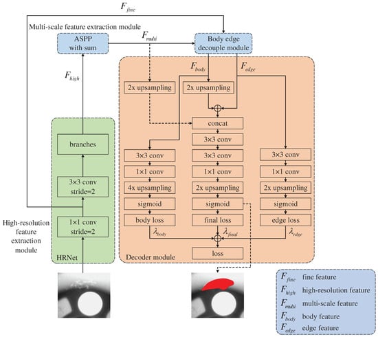
Figure 1. Surface defect detection network for automobile wheel hub.

3.1. High-Resolution Feature Extraction Module

In CNN, the commonly used backbone networks include VGGNet and ResNet. These backbone networks use many pooling layers, which help classify defects, but loses low-level spatial information, which is not conducive to the pixel detection in defect areas. HRNet can maintain a high-resolution feature with accurate spatial information and fuse the semantic information in the low-resolution feature, exhibiting a good defect segmentation effect. The resolution of the final feature map output from ResNet-101 is 1/32 of the original image, while that of the final feature map output from HRNet is 1/4 of the original image, which is nearer the original image resolution. When the feature map is restored to the original resolution, HRNet only needs four upsampling iterations, while ResNet-101 requires 32 upsampling iterations, indicating that HRNet as the backbone network can obtain a more accurate segmentation map than ResNet-101 [9].

HRNet is used on the image as the high-resolution feature extraction module. The structure of HRNet is shown in Figure 2.

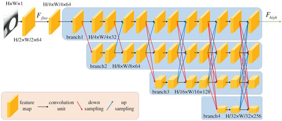
Figure 2. Structure of HRNet.

First, HRNet uses a convolution with a stride of 2 on the input image to obtain low-level feature $F_{fine}$, which contains fine image spatial information. Then, a convolution with a stride of 2 is used to extract a feature map whose resolution is 1/4 that of the original image. Next, this feature map is input into branch1, whose resolution is the highest among all the subnetworks. Finally, according to the order of resolution from high to low, the features are gradually input into the subnetworks for further feature extraction. After the repeat fusion of features with different resolutions in the four subnetworks, the feature maps from three other subnetworks are fused into branch1 to obtain the feature ($F_{high}$) to be output. $F_{high}$ has both high-resolution spatial and deep semantic classification information.

3.2. Multi-Scale Feature Extraction Module

DeepLab v3+ uses ASPP to detect defects of different sizes. ASPP uses atrous convolutions with different dilation rates, resulting in the gridding effect, which could cause local information loss and affect the classification results.

To address the gridding effect of atrous convolution based on the ASPP in DeepLab v3+, the article superimposes the features from ASPP to extract multi-scale features. The structure of the extraction module is shown in Figure 3.

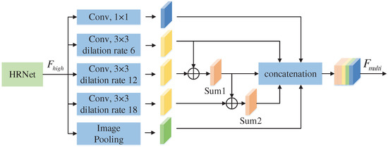
Figure 3. Multi-scale feature extraction module.

The specific steps are as follows:

1.

A 1 × 1 convolution, 3 × 3 atrous convolutions with dilation rates of 6, 12, and 18, and image pooling are used to extract different feature maps from high-resolution feature.

2.

The feature map (Sum1) is obtained by adding the two feature maps extracted by the 3 × 3 atrous convolutions with dilation rates of 6 and 12.

3.

The feature map extracted by atrous convolution with a dilation rate of 18 is added to feature map Sum1 to obtain feature map Sum2. In this way, feature maps Sum1 and Sum2 can obtain the features of different receptive fields to solve the gridding effect caused by atrous convolution.

4.

Finally, these five feature maps are concatenated, namely, Sum1, Sum2, and the feature maps from the 1 × 1 convolution and 3 × 3 atrous convolutions with dilation rates of 6 and image pooling. The final output ($F_{multi}$) contains information on the multi-scale and multiple receptive fields. Meanwhile, image pooling introduces global context information into $F_{multi}$, which improves the accuracy of defect segmentation.

3.3. Body and Edge Decoupling Module

The multi-scale feature of an image can be decoupled into two parts: the body and edge features of the low- and high-frequency parts, respectively, [31]. The body feature represents the internal association of objects in the image, and the edge feature represents the boundary difference between objects. Among these features, the multi-scale, body, and edge features meet the addition rule.

$$F_{multi}=F_{body}+F_{edge}$$

(1)

$F_{multi}$, $F_{body}$, and $F_{edge}$ represent the multi-scale, body, and edge features, respectively.

The optical flow can learn the positional relationship of each pixel in the same object between two frames, and a mutual relationship also exists between the feature points in the body feature of the defect image. Therefore, the body feature can be learned through the optical flow. The positional relationship can be found between the central and peripheral feature points of the same object, which is the optical flow field. To represent the body feature consistently and accurately, the central feature points are mapped to the positions of the corresponding peripheral feature points.

To generate optical flow field $\delta$, as shown in Figure 4, two 3 × 3 convolutions with a stride of 2 are used for downsampling. Using two consecutive convolutions can minimize the high-frequency information and enhance the body information representation of low-resolution features.

Figure 4. Generate optical flow field.

After downsampling $F_{multi}$, the feature map must be upsampled four times to obtain low-resolution feature $F_{flow}$ because its resolution is 1/4 that of $F_{multi}$. Similar to the input module of the optical flow network named FlowNet-Simple [32], a 3 × 3 convolution is used to extract the optical flow field after concatenating $F_{multi}$ and $F_{flow}$. Given that optical flow field $\delta$ is extracted based on $F_{multi}$, $\delta$ already contains a multi-scale feature, and a 3 × 3 convolution is sufficient to extract the feature between long-distance pixels.

After generating $\delta$, $F_{multi}$ is warped to obtain $F_{body}$.

$$F_{body}(x_2,y_2)=F_{body}(x_1+u_x,y_1+u_y)=F_{multi}(x_1,y_1)$$

(2)

As shown in Figure 5, $(x_1,y_1)$ represents the coordinate of the feature point in $F_{multi}$, and $(x_2,y_2)$ represents the coordinate of the feature point in $F_{body}$ warped from $F_{multi}$. $(u_x,u_y)$ represents the positional relationship of the feature points between $F_{multi}$ and $F_{body}$. According to the brightness constancy constraint, $F_{multi}(x_1,y_1)$ can be mapped to $F_{body}(x_2,y_2)$.

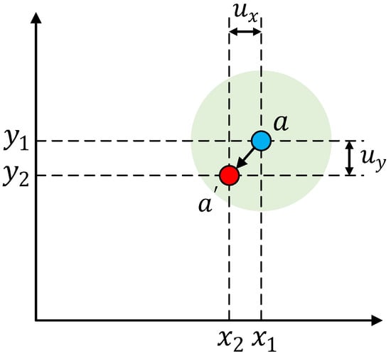
Figure 5. Warped multi-scale feature.

Given that $(x_1,y_1)$ is floating, $F_{multi}(x_1,y_1)$ is calculated by bilinear sampling.

$$F_{multi}\left(x_1,y_1\right)=\sum _{p\in N}{\omega }_p{F}_{multi}\left(p\right)$$

(3)

N represents the set of four feature points near $(x_1,y_1)$ in $F_{multi}$, p represents one of the points, and ${\omega }_p$ represents the bilinear kernel weight of p.

$F_{multi}$ is a deep feature and lacks boundary information in the low-level feature. If $F_{multi}$ is subtracted from $F_{body}$ to obtain $F_{edge}$ directly, $F_{edge}$ will also lack in boundary information, which will result in low accuracy in the boundary area.

After obtaining $F_{edge}$ by subtraction, the low-level feature ($F_{fine}$) extracted by the first convolution in HRNet is introduced into $F_{edge}$, which can introduce the missing boundary information to improve the accuracy in the boundary area. The process of extracting $F_{edge}$ can be formulated as Equation (4), and the network is shown in Figure 6.

$$F_{edge}=\gamma \left(concat(F_{multi}-F_{body}),\gamma \left(F_{fine}\right)\right)$$

(4)

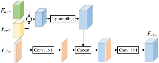
Figure 6. Network of extracting edge feature.

$\gamma$ represents convolution, and concat represents concatenation.

3.4. Decoder Module

As shown in Figure 7, the decoder module contains three branches, namely, the body feature optimization, edge feature optimization, and final feature merging branches.

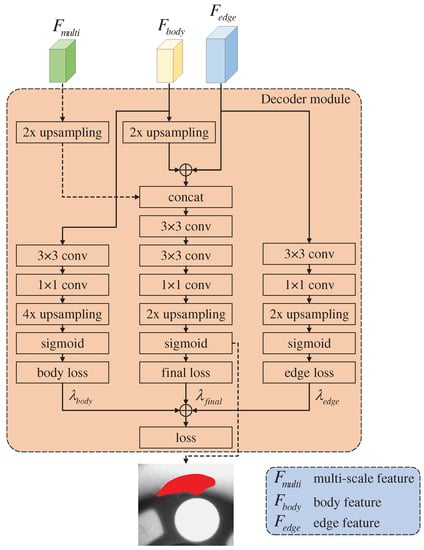
Figure 7. Decoder module.

3.4.1. Body Feature Optimization Branch

A 3 × 3 convolution and a 1 × 1 convolution are used to extract global information from $F_{body}$ and reduce the number of channels to two. Then, the obtained feature is upsampled (bilinear interpolation) four times and calculated using sigmoid to obtain the body segmentation map ($s_{body}$). According to $s_{body}$ and label $\widehat{s}$, weighted cross entropy loss is used to calculate the loss ($L_{body}$) of $F_{body}$.

$$L_{body}=-\frac{1}{N}\sum _{i=1}^N{\omega }_c·\left(y_{body,i}log{(p}_{body,i})+(1-y_{body,i})log(1-p_{body,i})\right)$$

(5)

$p_{body,i}$ is the probability that the pixel in $s_{body}$ is predicted to one class, and $y_{body,i}$ indicates whether the predicted class is consistent with the label. If the predicted class is consistent with the label, then $y_{body,i}$ is 1; otherwise, $y_{body,i}$ is 0. ${\omega }_c$ refers to the weight of the class for solving the imbalance from having fewer defect pixels than normal pixels. ${\omega }_c$ can be calculated using Equation (6).

$${\omega }_c=\frac{N-N_c}{N}$$

(6)

N indicates the number of all pixels, c indicates the class of pixel i, and $N_c$ indicates the number of all pixels belonging to c.

3.4.2. Edge Feature Optimization Branch

The setting of convolution in this branch is the same as that in the body feature optimization branch. Given that the resolution of $F_{edge}$ is 1/2 that of the original image, only double upsampling is required. Similar to Equation (5), weighted cross entropy loss is used to calculate the loss ($L_{edge}$) of $F_{edge}$ according to the edge segmentation map ($s_{edge}$) and label $\widehat{s}$:

$$L_{edge}=-\frac{1}{N}\sum _{i=1}^N{\omega }_c·\left(y_{edge,i}log{(p}_{edge,i})+(1-y_{edge,i})log(1-p_{edge,i})\right)$$

(7)

Through the body and edge feature optimization branches, supervision loss can be calculated so that the network can more accurately learn $F_{body}$ and $F_{edge}$ and improve the accuracy of defect edge detection.

3.4.3. Final Feature Merging Branch

First, the final feature merging branch adds $F_{body}$ and $F_{edge}$ to obtain the context feature, which contains body and edge information. Then, the context feature is concatenated with $F_{multi}$, which can introduce the correlation between $F_{body}$ and $F_{edge}$ lost when decoupling and effectively aggregate $F_{body}$ and $F_{edge}$. Next, two 3 × 3 convolutions are used for feature extraction to obtain the final feature ($F_{final}$). A 1 × 1 convolution is used to extract global information and reduce the number of channels to two. Finally, double upsampling and sigmoid are used to obtain the final segmentation map ($s_{final}$). Similar to Equation (5), weighted cross entropy loss is used to calculate the loss ($L_{final}$) of $F_{final}$ according to $s_{final}$ and label $\widehat{s}$:

$$\begin{array}{c}\hfill L_{final}=-\frac{1}{N}\sum _{i=1}^N{\omega }_c·\left(y_{final,i}log{(p}_{final,i})+(1-y_{final,i})log(1-p_{final,i})\right)\end{array}$$

(8)

To supervise $F_{final}$, $F_{body}$, and $F_{edge}$ simultaneously, the losses from the body feature optimization, edge feature optimization, and final feature merging branches are combined as the total loss (L) of the entire network. L can be formulated as Equation (9).

$$L={\lambda }_{final}{L}_{final}+{\lambda }_{body}{L}_{body}+{\lambda }_{edge}{L}_{edge}$$

(9)

$\lambda$ refers to the weight of each loss, which is set to 1 by default.

4. Experiments and Result Analyses

4.1. Datasets

In this study, we build a dataset of automobile wheel hub defect images to evaluate the performance of the proposed network. In addition, to verify whether the network can accurately detect defects from different products, three other public datasets are also used, namely, the magnetic tile [27], fabric [33], and weld defect datasets [31]. In order to make the network converge faster, the images of the input data set are cropped, denoised and normalized before the network training, so that the images have the same gray scale and resolution.

4.1.1. Automobile Wheel Hub Defect Dataset

The wheel hub images in this dataset are from the GDXray Casting dataset [31], and the wheels are aluminum. The original wheel defects in the GDXray Casting dataset are labeled with a bounding box and suitable for object detection, but not for semantic segmentation. We mark automobile wheel hub defects pixel-by-pixel to obtain labels that can be used for semantic segmentation.

The automobile wheel hub defect dataset includes 348 images, which cover four typical defects, namely, fray, hole, nick, and spot, as shown in Figure 8.

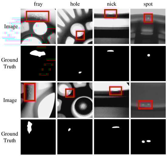
Figure 8. Images and ground truth of automobile wheel hub defect dataset.

4.1.2. Magnetic Tile Defect Dataset

Huang et al. [27] produced the magnetic tile defect dataset, including 1344 magnetic tile images cropped according to the ROI with defects. The defects of this dataset were divided into six categories, namely, blowhole, crack, break, fray, uneven, and free, as shown in Figure 9.

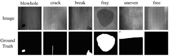
Figure 9. Images and the ground truth of magnetic tile defect dataset.

4.1.3. Fabric Defect Dataset

The fabric defect dataset is from the DAGM 2007 dataset [33]. We selected 2099 images from DAGM 2007, which includes 10 defect categories, as shown in Figure 10.

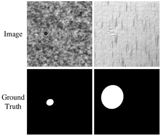
Figure 10. Images and the ground truth of fabric defect dataset.

4.1.4. Weld Defect Dataset

The weld defect dataset is from the GDXray dataset [31]. The dataset has 10 large X-ray images of metal pipes. Given that the width of the original image is much greater than the height, it is not suitable for direct input to the network, so the image must be cropped. After cropping, 192 images of welds were obtained, as shown in Figure 11.

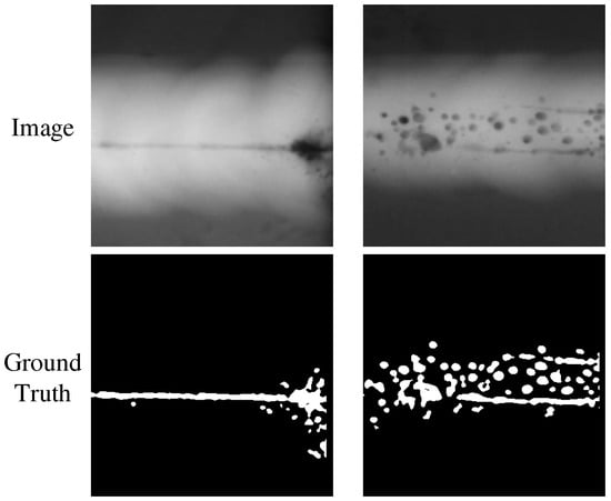
Figure 11. Images and the ground truth of weld defect dataset.

4.2. Evaluation Metrics

For each image, Precision and Recall can be calculated by comparing the detected defects with the ground truth. Then, the F1 score can be computed as an overall metric for performance evaluation.

$$Precision=\frac{TP+TN}{TP+TN+FP+FN}$$

(10)

$$Recall=\frac{TP}{TP+FN}$$

(11)

$$\mathrm{F}1=\frac{2\times Precision\times Recall}{Precision+Recall}$$

(12)

where TP (true positive) is correctly predicted positive examples; FP (false positive) is wrongly predicted negative examples; TN(true negative) is correctly predicted negative examples; FN(false negative) is wrongly predicted positive examples.

With precision as the vertical axis and recall as the horizontal axis, the precision–recall (PR) curve of the network can be obtained by changing the threshold for predicting a pixel as a defect. By calculating the area under the PR curve, the average precision (AP) of the network can also be obtained.

The IoU of the defect area is one of the evaluation metrics of semantic segmentation. IoU calculates the ratio of the intersection and union between the defect and normal areas. IoU can be formulated as Equation (13).

$$\mathrm{IoU}=\frac{TP}{TP+FN+FP}$$

(13)

4.3. Implementation Details

We use the PyTorch [34] framework to carry out the following experiments. The backbone network used is HRNet-W32, where 32 represents the channel factor of the branch in HRNet. For HRNet-W32, the channel numbers of the four branches are 32, 64, 128, and 256. When training the network, SGD is used to update the network parameters, with a weight decay of 0.0001, a momentum of 0.9, an epoch of 160, and an initial learning rate of 0.01 and using the poly learning rate strategy. The resolution of the input image is 512 × 512. All the experiments were performed on a single Nvidia GeForce GTX 2080Ti.

4.4. Experimental Results

4.4.1. Overall Performance

In Figure 12, the first column is the wheel image, the second to fifth columns are the detect maps of SegNet, Unet, DeepLab v3+, and the proposed network, and the sixth column is the ground truth. The detect maps of SegNet and DeepLab v3+, have some white dots outside marked by white boxes, indicating that SegNet and DeepLab v3+ are overfitting and some normal pixels are detected as defect pixels. In the detect maps of Unet and the proposed network, such white dots are gradually reduced. Furthermore, the area of defects detected in the proposed network is gradually reduced compared with that in Unet, indicating that the proposed network can effectively reduce the false detection rate of defects.

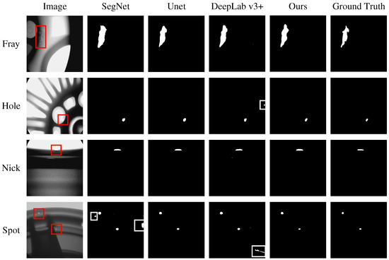
Figure 12. Wheel hub defect maps detected by different networks. White boxes are the mistakes.

As shown in Figure 13, the proposed network also has better detect effects on the three defect datasets (tile, fabric, and weld) than the other networks, indicating that it is suitable for different detection scenarios.

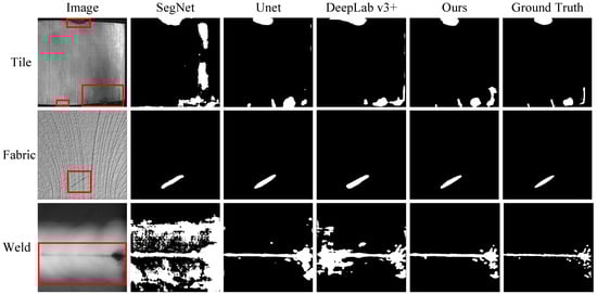
Figure 13. Defect maps detected by different networks on three defect datasets of tile, fabric, and weld.

Figure 14 shows the PR curves of SegNet, Unet, DeepLab v3+, and the proposed network on the four defect datasets. On the three defect datasets (tile, fabric, and weld), the PR curves of the proposed network are significantly better than those of the other networks. On the weld defect dataset, when the recall is small, the PR curve of the proposed network is near the PR curves of Unet and DeepLab v3+, but when the recall is large, the PR curve of the proposed network is better than those of Unet and DeepLab v3+, and the AP of the proposed network is greater than those of Unet and DeepLab v3+, indicating that the proposed network is also better than the other networks on the weld defect dataset.

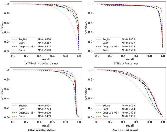
Figure 14. Comparison of PR curves and AP on four defect datasets.

As shown in Table 1, the proposed network achieved better results (i.e., F1 score, AP, and IoU) on the four defect datasets (wheel, tile, fabric, and weld) than SegNet, Unet, and DeepLab v3+. On the wheel defect dataset, the proposed network improved the F1 score, AP, and IoU of DeepLab v3+ by 6.2%, 2.1%, and 8.4%, respectively, indicating that using HRNet as the backbone network, introducing ASPP with sum (superimposing features), and using a body and edge decoupling module and a decoder can help the network extract high-resolution, multi-scale, and edge features. These modules can improve the accuracy of detecting automobile wheel hub defects.

Table 1. F1 score, AP, and IoU (%) of different networks on four defect datasets.

Methods	Wheel Hub			Tile			Fabric			Weld
	F1	AP	IoU	F1	AP	IoU	F1	AP	IoU	F1	AP	IoU
SegNet	0.748	0.863	60.6	0.643	0.935	51.8	0.762	0.906	64.7	0.426	0.675	27.1
Unet	0.757	0.936	61.6	0.772	0.943	64.6	0.847	0.924	73.7	0.591	0.761	41.9
DeepLab v3+	0.783	0.942	64.8	0.709	0.942	57.9	0.807	0.908	69.0	0.564	0.752	39.2
Ours	0.845	0.963	73.2	0.844	0.954	73.9	0.858	0.944	75.3	0.729	0.783	57.3

On the challenging weld defect dataset, the proposed network improves the F1 score, AP, and IoU of DeepLab v3+ by 16.5%, 3.1%, and 18.1%, respectively. The obvious improvement proves the accuracy of the proposed network on other defect detection scenarios.

4.4.2. Performance Improvement by Each Module

Figure 15 shows that after introducing each module based on DeepLab v3+, the detected boundaries are nearer the boundaries in the ground truth than before the modules were applied, indicating that each module successfully improved the detect accuracy.

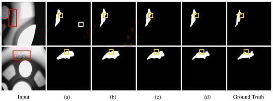
Figure 15. On the wheel hub defect dataset, performance improvement by each module on the basis of DeepLab v3+. (a) defect maps of DeepLab v3+; (b) detect maps after using HRNet; (c) detect maps after using ASPP with sum; and (d) detect maps after using body and edge decoupling module and decoder module. The red boxes are the defect positions, the white boxes are the mistake positions, and the yellow boxes are the boundary positions of the defect.

Table 2 shows that after importing each module in turn, F1 score and IoU improved greatly compared with those using DeepLab v3+.

Table 2. Improvement of F1 score and IoU by each module.

(a) Improvement of F1 Score
Method	Wheel hub		Tile		Fabric		Weld
	F1	$\Delta$(%)	F1	$\Delta$(%)	F1	$\Delta$(%)	F1	$\Delta$(%)
DeepLab v3+	0.783	-	0.709	-	0.807	-	0.564	-
+HRNet	0.8	1.7↑	0.782	7.3↑	0.847	4.0↑	0.689	12.5↑
+ASPP with sum	0.805	0.5↑	0.816	3.4↑	0.852	0.5↑	0.726	3.7↑
+Decouple and Decoder	0.845	4.0↑	0.844	2.8↑	0.858	0.6↑	0.729	0.3↑
(b) Improvement of IoU
Method	Wheel hub		Tile		Fabric		Weld
	IoU(%)	$\Delta$(%)	IoU(%)	$\Delta$(%)	IoU(%)	$\Delta$(%)	IoU(%)	$\Delta$(%)
DeepLab v3+	64.8	-	57.9	-	69	-	39.2	-
+HRNet	66.4	1.6↑	65.1	7.2↑	73.8	4.8↑	52.6	13.4↑
+ASPP with sum	67.6	1.2↑	70.2	5.1↑	74.7	0.9↑	57	4.4↑
+Decouple and Decoder	73.2	5.6↑	73.9	3.7↑	75.3	0.6↑	57.3	0.3↑

The defects of the tile and weld defect datasets have a more irregular appearance and larger scale changes than those of the other datasets. Using HRNet and introducing ASPP with sum greatly improved F1 score and IoU, verifying that HRNet can improve the feature resolution and ASPP with sum helps extract multi-scale features and solve the gridding effect.

In the wheel and tile defect datasets, the appearance of the defect boundary is more similar to the normal area than the other datasets. After using the body and edge decoupling module and decoder, F1 score and IoU improved significantly, proving that the body and edge decoupling module can accurately extract edge features and improve the detection accuracy in the boundary area, and the decoder can effectively merge the body, edge, and multi-scale features to restore an accurate segmentation map. Notably, the appearance of defects in the weld defect dataset is simpler than that in other datasets, and the detection effect of the body and edge decoupling module cannot greatly improve the detection effect on the weld dataset.

As shown in Figure 16, after introducing each module, the PR curve became nearer the upper right corner, and the AP continued to increase, indicating that the various proposed modules have an improved effect on defect detection.

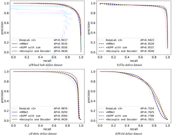
Figure 16. Improvement of PR curve and AP by each module.

4.4.3. Performance Improvement by Each Module

The total loss of the proposed network consists of three parts: final feature loss $L_{final}$, body feature loss $L_{body}$, and edge feature loss $L_{edge}$. Different weight settings for each loss will affect the performance of the network differently. The experiments indicate that $L_{edge}$ is much higher than $L_{final}$ and $L_{body}$, which results in an extremely large proportion of $L_{edge}$ in the total loss, causing the network to fail to learn the final and body features well. Therefore, the weight (${\lambda }_{edge}$) of $L_{edge}$ must be small, but an extremely small weight will also cause the network to fail to learn the edge feature well. Experiments were conducted to explore the impact of different loss weight settings on network performance and find an ideal setting. Given that $L_{final}$ is near $L_{body}$, the final feature loss weight (${\lambda }_{final}$) and the body feature loss weight (${\lambda }_{body}$) can be fixed to 1. For ${\lambda }_{edge}$, several representative weights were selected: 0.01, 0.05, 0.1, 0.5, and 1. Experiments were conducted on the wheel defect dataset, and the results are shown in Table 3.

Table 3. Influence of different loss weight settings on F1 score and IoU on the wheel defect dataset.

{${\mathit{\lambda }}_{\mathit{final}}$, ${\mathit{\lambda }}_{\mathit{body}}$, ${\mathit{\lambda }}_{\mathit{edge}}$}	F1	IoU (%)
{1, 1, 1}	0.833	71.5
{1, 1, 0.5}	0.841	72.6
{1, 1, 0.1}	0.845	73.2
{1, 1, 0.05}	0.826	70.5
{1, 1, 0.01}	0.823	70

In Table 3, when ${\lambda }_{edge}$ gradually decreases from 1 to 0.1, F1 score and IoU will gradually increase; when ${\lambda }_{edge}$ gradually decreases from 0.1 to 0.01, F1 score and IoU will gradually decrease. The experimental result shows that ${\lambda }_{edge}$ needs to be set to a smaller value than ${\lambda }_{final}$ and ${\lambda }_{body}$. When ${\lambda }_{edge}$ is set to 0.1, the defect detection effect is better than other settings.

4.4.4. Comparison of Different Sample Sizes

The original automobile wheel hub defect dataset contains 348 image samples, and convolutional neural network often requires a large sample size. To explore the influence of different sample sizes on the performance of the defect detection network, this section increases sample size by data enhancement, such as rotating, flipping and cropping. After data enhancement, sample sizes are expanded to 3 times, 6 times and 9 times. Then, experiments were conducted on the wheel defect datasets with sample sizes of 348, 1044, 2088, and 3132.

As shown in Figure 17, when sample size increased from 348 to 3132, F1 score increased by 2.54% and IoU increased by 3.9%, indicating that the increase in sample size can improve the detection performance of the defect detection network. Furthermore, when sample size is small, the defect detection network still has a high F1 score and IoU, indicating that the defect detection network still has accurate detection performance in the small sample size.

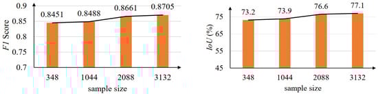
Figure 17. Influence of different sample sizes on F1 score and IoU on the wheel defect dataset.

When sample size increased from 2088 to 3132, the improvement of detection performance was small, but the training time was greatly increased because sample size was increased. When sample size was 2088, a balance between detection performance and training time was achieved.

5. Conclusions

In this paper, we proposed semantic segmentation network for the surface defect detection of automobile wheel hub. ASPP based on feature superposition design avoids the gridding effect of atrous convolution. The body and edge decoupling module can extract edge features for accurate boundary detection. In addition, the improved decoder module combines the body, edge and multi-scale features. The comprehensive experimental results have demonstrated that the proposed semantic segmentation network could effectively extract high-resolution and multi-scale features in defect images and it is also suitable for defect detection tasks of different industrial products.

The actual defects detection of automobile wheel hub often has higher requirements on the detection speed and anti-interference ability of the semantic segmentation network. In order to be able to deploy it in actual defect detection scenarios, we will continue to conduct in-depth research on weakly supervised learning, improving real-time performance, and improving the robustness of the semantic segmentation network.

References

- Sun, X.; Gu, J.; Huang, R.; Zou, R.; Giron Palomares, G. Surface Defects Recognition of Wheel Hub Based on Improved Faster R-CNN. Electronics 2019, 8, 481. [Google Scholar] [CrossRef] [Green Version]
- Jiang, L.; Sun, K.; Zhao, F.; Hao, X. Automatic Detection System of Shaft Part Surface Defect Based on Machine Vision. In Conference on Automated Visual Inspection and Machine Vision; International Society for Optics and Photonics: Bellingham, WA, USA, 2015; Volume 9530, p. 9530G. [Google Scholar]
- Chauhan, A.P.S.; Bhardwaj, S.C. Detection of Bare PCB Defects by Image Subtraction Method using Machine Vision. Lect. Notes Eng. Comput. Sci. 2011, 2, 6–8. [Google Scholar]
- Han, Y.; Wu, Y.; Cao, D.; Yun, P. Defect detection on button surfaces with the weighted least-squares model. Front. Optoelectron. 2017, 10, 151–159. [Google Scholar] [CrossRef]
- Çelik, H.İ.; Dülger, L.C.; Topalbekiroğlu, M. Development of a machine vision system: Real-time fabric defect detection and classification with neural networks. J. Text. Inst. 2014, 105, 575–585. [Google Scholar] [CrossRef]
- Yi, L.; Li, G.; Jiang, M. An End-to-End Steel Strip Surface Defects Recognition System Based on Convolutional Neural Networks. Steel Res. Int. 2017, 88, 1600068. [Google Scholar] [CrossRef]
- Ren, R.; Hung, T.; Tan, K.C. A Generic Deep-Learning-Based Approach for Automated Surface Inspection. IEEE Trans. Cybern. 2018, 48, 929–940. [Google Scholar] [CrossRef] [PubMed]
- Han, K.; Sun, M.; Zhou, X.; Zhang, G.; Dang, H.; Liu, Z. A new method in wheel hub surface defect detection: Object detection algorithm based on deep learning. In Proceedings of the 2017 International Conference on Advanced Mechatronic Systems (ICAMechS), Xiamen, China, 6–9 December 2017; pp. 335–338. [Google Scholar]
- He, K.; Zhang, X.; Ren, S.; Sun, J. Deep Residual Learning for Image Recognition. In Proceedings of the IEEE Conference on Computer Vision and Pattern Recognition (CVPR), Las Vegas, NV, USA, 27–30 June 2016. [Google Scholar]
- He, Y.; Song, K.; Meng, Q.; Yan, Y. An End-to-End Steel Surface Defect Detection Approach via Fusing Multiple Hierarchical Features. IEEE Trans. Instrum. Meas. 2020, 69, 493–1504. [Google Scholar] [CrossRef]
- Tellaeche Iglesias, A.; Campos Anaya, M.Á.; Pajares Martinsanz, G.; Pastor-López, I. On Combining Convolutional Autoencoders and Support Vector Machines for Fault Detection in Industrial Textures. Sensors 2021, 21, 3339. [Google Scholar] [CrossRef] [PubMed]
- Jaffari, R.; Hashmani, M.A.; Reyes-Aldasoro, C.C.; Aziz, N.; Rizvi, S.S.H. Deep Learning Object Detection Techniques for Thin Objects in Computer Vision: An Experimental Investigation. In Proceedings of the 2021 7th International Conference on Control, Automation and Robotics (ICCAR), Singapore, 23–26 April 2021; pp. 295–302. [Google Scholar]
- Dong, Z.; Wang, J.; Cui, B.; Wang, D.; Wang, X. Patch-based weakly supervised semantic segmentation network for crack detection. Constr. Build. Mater. 2020, 258, 120291. [Google Scholar] [CrossRef]
- Long, J.; Shelhamer, E.; Darrell, T. Fully Convolutional Networks for Semantic Segmentation. IEEE Trans. Pattern Anal. Mach. Intell. 2014, 39, 640–651. [Google Scholar]
- Badrinarayanan, V.; Kendall, A.; Cipolla, R. SegNet: A Deep Convolutional Encoder-Decoder Architecture for Scene Segmentation. IEEE Trans. Pattern Anal. Mach. Intell. 2017, 12, 2481–2495. [Google Scholar] [CrossRef] [PubMed]
- Ronneberger, O.; Fischer, P.; Brox, T. U-Net: Convolutional Networks for Biomedical Image Segmentation. In Medical Image Computing and Computer-Assisted Intervention; Springer: Cham, Switzerland, 2015; pp. 234–241. [Google Scholar]
- Chen, L.C.; Zhu, Y.; Papandreou, G.; Schroff, F.; Adam, H. Encoder-Decoder with Atrous Separable Convolution for Semantic Image Segmentation. In Proceedings of the IEEE Conference on Computer Vision and Pattern Recognition, Munich, Germany, 8–14 September 2018; pp. 801–818. [Google Scholar]
- Li, X.; Zhang, L.; Li, X.; Cheng, G.; Shi, J.; Lin, Z.; Tan, S.; Tong, Y. Improving Semantic Segmentation via Decoupled Body and Edge Supervision. In Proceedings of the European Conference on Computer Vision, Glasgow, UK, 23–28 August 2020; pp. 435–452. [Google Scholar]
- Zhou, B.; Khosla, A.; Lapedriza, A.; Oliva, A.; Torralba, A. Object detectors emerge in deep scene cnns. arXiv 2014, arXiv:1412.6856. [Google Scholar]
- Luo, W.; Li, Y.; Urtasun, R.; Zemel, R. Understanding the effective receptive fieldin deep convolutional neural networks. In Proceedings of the 30th International Conference on Neural Information Processing Systems, Barcelona, Spain, 5–10 December 2016. [Google Scholar]
- Sun, K.; Xiao, B.; Liu, D.; Wang, J. Deep High-Resolution Representation Learning for Human Pose Estimation. In Proceedings of the IEEE/CVF Conference on Computer Vision and Pattern Recognition (CVPR), Long Beach, CA, USA, 16–20 June 2019; pp. 5693–5703. [Google Scholar]
- Yu, Z.; Wu, X.; Gu, X. Fully Convolutional Networks for Surface Defect Inspection in Industrial Environment. In International Conference on Computer Vision Systems; Springer: Cham, Switzerland, 2017; pp. 417–426. [Google Scholar]
- Dung, C.V. Autonomous concrete crack detection using deep fully convolutional neural network. Autom. Constr. 2019, 99, 52–58. [Google Scholar] [CrossRef]
- Dong, Y.; Wang, J.; Wang, Z.; Zhang, X.; Gao, Y.; Sui, Q.; Jiang, P. A Deep-Learning Based Multiple Defect Detection Method for Tunnel Lining Damages. IEEE Access 2019, 7, 182643–182657. [Google Scholar] [CrossRef]
- Roberts, G.; Haile, S.Y.; Sainju, R.; Edwards, D.J.; Hutchinson, B.; Zhu, Y. Deep Learning for Semantic Segmentation of Defects in Advanced STEM Images of Steels. Sci. Rep. 2019, 9, 1–12. [Google Scholar] [CrossRef] [PubMed] [Green Version]
- Zou, Q.; Zhang, Z.; Li, Q.; Qi, X.; Wang, Q.; Wang, S. DeepCrack: Learning Hierarchical Convolutional Features for Crack Detection. IEEE Trans. Image Process. 2018, 28, 1498–1512. [Google Scholar] [CrossRef] [PubMed]
- Huang, Y.; Qiu, C.; Yuan, K.; Wang, X.; Yuan, K. Surface Defect Saliency of Magnetic Tile. In Proceedings of the International Conference on Automation Science and Engineering, Munich, Germany, 20–24 August 2018; pp. 612–617. [Google Scholar]
- Li, S.; Zhao, X.; Zhou, G. Automatic pixel-level multiple damage detection of concrete structure using fully convolutional network. Comput.-Aided Civ. Infrastruct. Eng. 2019, 34, 616–634. [Google Scholar] [CrossRef]
- Liu, E.; Chen, K.; Xiang, Z.; Zhang, J. Conductive particle detection via deep learning for ACF bonding in TFT-LCD manufacturing. J. Intell. Manuf. 2020, 31, 1037–1049. [Google Scholar] [CrossRef]
- Nie, Z.; Xu, J.; Zhang, S. Analysis on DeepLabV3+ Performance for Automatic Steel Defects Detection. arXiv 2020, arXiv:2004.04822. [Google Scholar]
- Mery, D.; Riffo, V.; Zscherpel, U.; Mondragón, G.; Lillo, I.; Zuccar, I.; Lobel, H.; Carrasco, M. GDXray: The database of X-ray images for nondestructive testing. J. Nondestruct. Eval. 2015, 34, 1–12. [Google Scholar] [CrossRef]
- Dosovitskiy, A.; Fischer, P.; Ilg, E.; Hazırbaş, C.; Golkov, V.; Smagt, P.; Cremers, D.; Brox, T. FlowNet: Learning Optical Flow with Convolutional Networks. In Proceedings of the IEEE International Conference on Computer Vision (ICCV), Santiago, Chile, 7–13 December 2015; pp. 2758–2766. [Google Scholar]
- Perwass, C. DAGM 2007 Symposium. 2007. Available online: http://www.address_of_you_wannar_cite/ (accessed on 25 December 2019).
- Paszke, A.; Gross, S.; Chintala, S.; Chanan, G. Automatic differentiation in PyTorch. In Proceedings of the Conference on Neural Information Processing Systems, Long Beach, CA, USA, 4–9 December 2017; pp. 1–4. [Google Scholar]
Publisher’s Note: MDPI stays neutral with regard to jurisdictional claims in published maps and institutional affiliations. |
© 2021 by the authors. Licensee MDPI, Basel, Switzerland. This article is an open access article distributed under the terms and conditions of the Creative Commons Attribution (CC BY) license (https://creativecommons.org/licenses/by/4.0/).