Stability of Traveling Waves Based upon the Evans Function and Legendre Polynomials

Abstract

One of the tools and techniques concerned with the stability of nonlinear waves is the Evans function which is an analytic function whose zeros give the eigenvalues of the linearized operator. Here, in this paper, we propose a direct approach, which is based essentially upon constructing the eigenfunction solution of the perturbed equation based upon the topological invariance in conjunction with usage of the Legendre polynomials, which have presumably not considered in the literature thus far. The associated Legendre eigenvalue problem arising from the stability analysis of traveling waves solutions is systematically studied here. The present work is of considerable interest in the engineering sciences as well as the mathematical and physical sciences. For example, in chemical industry, the objective is to achieve a great yield of a given product. This can be controlled by depicting the initial concentration of the reactant, which is determined by its value at the bifurcation point. This analysis leads to the point separating stable and unstable solutions. As far as chemical reactions are described by reaction-diffusion equations, this specific concentration can be found mathematically. On the other hand, the study of stability analysis of solutions may depict whether or not a soliton pulse is well-propagated in fiber optics. This can, and should, be carried out by finding the solutions of the coupled nonlinear Schrödinger equations and by analyzing the stability of these solutions.

1. Introduction

In what follows, we distinguish between stationary waves (pulses) and wave fronts. A traveling wave $Q\left(z\right)$$(z=x-ct)$ is a front if it travels at speed $c\ne 0$ and

$$\underset{z\to \pm \in }{lim}Q\left(z\right)=Q_{\pm }.$$

On the other hand, for a stationary pulse (with $c=0$) and

$$\underset{z\to \pm \in }{lim}Q\left(z\right)=Q_0.$$

In order to determine the stability of the solutions of a given partial differential equation, we linearize it about the wave solution. Then, with a view to recognizing the stability, it suffices to determine that the spectrum in the left-half plane ($\Re \left(\alpha \right)<0$) corresponds to stable places and that the spectrum in the right-half plane ($\Re \left(\alpha \right)>0$) corresponds to unstable places. There are many applications of the Legendre polynomials as they arise in mathematical models of the heat conduction and fluid flow problems in spherical coordinates. The novelty of the proposed method via the finding of the eigenvalues exactly is shown in Section 4. This is the advantage of our proposed method over a previous method (see, for details [1]).

This paper is constructed as follows. It is devoted to a systematic study of the stability of traveling waves through the use of the exponential dichotomies and the Evans function. In Section 2, we will discuss the stability of pulses. In Section 3, we illustrate the results by considering two examples. In Section 4, we will introduce the direct approach for analyzing the stability of traveling wave solutions and compute the eigenvalues for the associated Legendre equation arising from the stability analysis of traveling waves after making a convenient transformation. Finally, conclusions will be presented in Section 4.

We first introduce the stability analysis of these waves by using exponential dichotomies.

1.1. Exponential Dichotomies

First of all, we consider the following set of first-order ordinary differential equations:

$$\frac{d\overrightarrow{u}}{dz}=A\left(\alpha \right)\overrightarrow{u}(\overrightarrow{u}={(u_1,u_2,\cdots ,u_n)}^T),$$

(1)

where

$$A={(a_{ij}(\alpha ))}_{n\times n},$$

$$\overrightarrow{u}\in {ℝ}^n\mathrm{or}\overrightarrow{u}\in {ℂ}^n$$

and

$$A\in {ℝ}^{n\times n}\mathrm{or}A\in {ℂ}^{n\times n}.$$

If the eigenvalues of the matrix A have nonzero real parts, then the space ${ℝ}^n$ or ${ℂ}^n$ is split into two stable or unstable eigenspaces according to whether the real parts of the eigenvalues are negative or positive, respectively. Equation (1) has an exponential dichotomy on a subspace of $ℝ$ with the following evaluation:

$$\varphi (z,z_0)=e^{A\left(\alpha \right)(z-z_0)},$$

where

$$u\left(z\right)=\varphi (z,z_0)u(z_0).$$

Now, for the Equation (1), we have

$$\frac{d\overrightarrow{u}}{dz}=A\left(z\right)\overrightarrow{u}\mathrm{and}A\in {ℂ}^0(I,{ℂ}^{n\times n}),$$

(2)

where

$$I={ℝ}^{+}(\mathrm{or}{ℝ}^{-}\mathrm{or}ℝ).$$

A fundamental set of solutions of the Equation (2) is a set of n linearly independent vectors ${\overrightarrow{u}}_1\left(z\right),{\overrightarrow{u}}_2\left(z\right),\cdots ,{\overrightarrow{u}}_n\left(z\right)$. The square matrix $K\left(z\right)$, which is constructed with columns consisting of the vectors ${\overrightarrow{u}}_1\left(z\right),{\overrightarrow{u}}_2\left(z\right),\cdots ,{\overrightarrow{u}}_n\left(z\right),$ is the fundamental matrix of the differential Equation (2). We then have the following representation (see [2]):

$$\overrightarrow{u}\left(z\right)=K(z){[K(z_0)]}^{-1}\overrightarrow{u_0}$$

(3)

and

$$\det K\left(z\right)=\det K(z_0)e^{{\int }_{z_0}^z\mathrm{Tr}A\left(Z\right)dZ},$$

(4)

where

$$\overrightarrow{u_0}=\overrightarrow{u}(z_0).$$

Equation (4) for the determinant of the fundamental matrix may serve as an introductory definition of the Evans function.

1.2. Evans Function

The Evans function is an important tool for studying and investigating the stability of nonlinear waves (see, for example, [3,4]). The Evans function is an analytic function whose zeros correspond exactly, in location and multiplicity, to the eigenvalues of the linearized operator. The Evans function was first formulated by Evans for a specific class of systems and is a generalization which is suited for systems of partial differential equations of the transmission coefficient from quantum mechanics (see, for details, [5,6,7]). Evans paid remarkable attention toward studying the stability of nerve impulses, which he then classified as the category of nerve impulse equations. This class has an important property that leads naturally to the formulation of blue the Evans function in a clear and straightforward manner. The $D\left(\alpha \right)$ notation was used by Evans to refer to the determinant which, in fact, played the same role as the determinant of an eigenvalue matrix in problems of finite dimensions. Jones in [8] applied the stability of the traveling pulse (nerve impulse) of the Fitzhugh-Nagumo system by following Evans’ idea. In fact, Jones gave the name “Evans function" as well as the notation $E\left(\alpha \right)$ which is now in common usage. The authors in [9] presented the first general definition of the Evans function $E\left(\alpha \right)$, which is based upon the idea of Evans, with its placement in a new conceptual form to clearly give a general definition.

We consider the following eigenvalue problem:

$$\frac{d\overrightarrow{u}}{dz}=A(z;\alpha )\overrightarrow{u}(\overrightarrow{u}\in {ℝ}^n(\mathrm{or}{ℂ}^n);-\in <z<\in )$$

(5)

and assume that (5) is rewritten in the form given by

$$\frac{d\overrightarrow{u}}{dz}=(A_0\left(\alpha \right)+A_1\left(z\right))\overrightarrow{u}.$$

(6)

Firstly, we consider the following equation:

$$\frac{d\overrightarrow{u}}{dz}=A_0\left(\alpha \right)\overrightarrow{u}\left(\alpha \in ℝ(\mathrm{or}ℂ)\right)$$

(7)

and assume that the eigenvalues of $A_0\left(\alpha \right)$ are ${\beta }_1\left(\alpha \right),{\beta }_2\left(\alpha \right),\cdots ,{\beta }_n\left(\alpha \right)$ and that the corresponding eigenvectors are ${\gamma }_1\left(\alpha \right),{\gamma }_2\left(\alpha \right),\cdots ,{\gamma }_n\left(\alpha \right).$ Whenever $\Re ({\beta }_j)\ne 0$ and the ${\beta }_j$ are distinct for $j=1,\cdots ,n,$ the space ${ℂ}^n$ is represented as follows:

$${ℂ}^n=E^s\oplus E^u.$$

We assume that

$$\Re ({\beta }_j)<0(j=1,\cdots ,k)$$

and that

$$\Re ({\beta }_j)>0(j=k+1,\cdots ,n),$$

while

$$E^s=\{{\overrightarrow{u}}_j\left(\alpha \right)\mathrm{and}\Re ({\beta }_j\left(\alpha \right))<0(j=1,\cdots ,k)\}$$

and

$$E^u=\{{\overrightarrow{u}}_j\left(\alpha \right)\mathrm{and}\Re ({\beta }_j\left(\alpha \right))>0(j=k+1,\cdots ,n)\}.$$

Solutions belonging to $E^s$ are bounded as $z\to \in$, while the solutions belonging to $E^u$ are bounded as $z\to -\in .$ We may then label these solutions as $u_j^{+}\left(\alpha \right)$ or $u_j^{-}\left(\alpha \right)$, according to whether they are bounded as $z\to \in$ or $z\to -\in .$ Also, these solutions satisfy the following limit relationship:

$$\underset{z\to \pm \in }{lim}{\overrightarrow{u}}_j^{\pm }(z,\alpha )e^{{\beta }^{\mp }\left(\alpha \right)z}={\gamma }^{\mp }.$$

(8)

We mention that there exist a set of values ${\alpha }_0$ and a common subspace of $E^s$ and $E^u$ such that

$$\underset{z\to \pm \in }{lim}\overrightarrow{u}(z,{\alpha }_0)=0.$$

We now give the following definition.

Definition 1.

$\alpha ={\alpha }_0\in ℂ$is an eigenvalue of (5) if the following condition holds true:

$$\underset{z\to \pm \in }{lim}{\overrightarrow{u}}_j^{\pm }(z,{\alpha }_0)=0.$$

(9)

We mention here that the values of $\alpha ,$ which satisfy the equation $\Re ({\beta }_j\left(\alpha \right))=0$ determines the essential spectrum of the Equation (5).

The spectrum of the Equation (5) generally consists of the pure point spectrum, isolated eigenvalues of finite multiplicity, and the essential spectrum. The essential spectrum is contained within the parabolic curves of the continuous spectrum (see [10]). In many cases, the essential spectrum can be shown to be contained in the left-half complex plane and hence does not contribute to linear instability. Now, we search for solutions of the Equation (5), namely

$$\frac{d{\overrightarrow{u}}_i^{\pm }}{dz}=A(z,\alpha ){\overrightarrow{u}}^{\pm },$$

(10)

together with the boundary conditions given by

$$\underset{z\to \pm \in }{lim}u(z,{\alpha }_0)=0.$$

The Evans function is defined after the solutions of (11) as follows:

$$E\left(\alpha \right)=e^{-{\int }_0^z\mathrm{Tr}A(Z,\alpha )dZ}\det (u_{\ell }^{+}(\alpha ,z),u_j^{-}(\alpha ,z)),$$

(11)

where $\ell =1,\cdots ,k$ and $j=k+1,\cdots ,n.$ As a consequence of Abel’s formula, the Evans function $E\left(\alpha \right)$ given by (11) is independent of z and $E\left(0\right)=0.$ By fixing the orientation of the orthonormal basis of the subspaces $E^s$ and $E^u$, the Evans function can be made unique and the following theorem holds true (see [2,6,9,11]).

Theorem 1.

The Evans function$E\left(\alpha \right)$is analytic on$\{\Re (\alpha )\geqq 0\}$and satisfies the following properties:

(i) 

$E\left(\alpha \right)\in ℝ$whenever$\alpha \in \{\Re (\alpha )\geqq 0\}.$

(ii) 

$E\left(\alpha \right)=0$if and only if α is an eigenvalue of (5)

(iii) 

The order of${\alpha }_{*}$as a zero of the Evans function$E\left(\alpha \right)$is equal to the algebraic multiplicity of${\alpha }_{*}$as an eigenvalue of (5)

In applications, one finds that $\mathrm{Tr}A(z,\alpha )=0,$ so that the Evans function $E\left(\alpha \right)$ reduces to

$$E\left(\alpha \right)=\det \left({\overrightarrow{u}}^{-}(z,\alpha ),{\overrightarrow{u}}^{+}(z,\alpha )\right).$$

The importance of the manner in which the Evans function $E\left(\alpha \right)$ is constructed is seen by the following argument. Suppose that $E\left({\alpha }_0\right)=0$ for some ${\alpha }_0$. It is then clear that

$${\overrightarrow{u}}^{-}({\alpha }_0,x)=\gamma {\overrightarrow{u}}^{+}({\alpha }_0,x)$$

for some $\gamma \in ℂ$. Hence, clearly, there is a localized solution of the Equation (10) when $\alpha ={\alpha }_0$, such that ${\alpha }_0$ is an eigenvalue. Similarly, if ${\alpha }_0$ is an eigenvalue, then it is not difficult to convince oneself that $E({\alpha }_0)=0.$ In general, the Equation (11) is not explicitly given as a function of $\alpha .$ It is then necessary to evaluate the Evans function numerically (see, for details, [1,12,13,14,15,16]). In this case, the boundary conditions for the Equation (10) are approximately used at infinity by approximating the boundary conditions (see [17]). An alternative approximation is to set the Equation (10) on a bounded domain, namely, on $L_{-\in }\leqq z\leqq 0$ and $0\leqq z\leqq L_{\in }$, and then impose the exact asymptotic boundary conditions for boundedness of the solution of the Equation (10) at these finite end-points. The use of approximate boundary conditions usually has a dramatic impact on the essential (continuous) spectrum (see [18]). One of the most useful numerical techniques is the exterior numerical computations of discrete eigenvalues of the Equation (10), which has no effect on the essential spectrum (see [18]). In this case, the exact boundary conditions are applied at finite values $L_{\pm \in },$ which are taken to be sufficiently large (see [19]). In the extended space of exterior products, the Equation (11) becomes

$$\frac{d{\overrightarrow{U}}^{\pm }}{dz}=A^{\left(k\right)}(z,\alpha ){\overrightarrow{U}}^{\pm }\mathrm{and}{U}^{\pm }{(z,\alpha )|}_{z\to L_{\pm \in }}=b\left(\alpha \right)\in {\wedge }^k({ℂ}^n),$$

(12)

where

$$A^{\left(k\right)}U=\sum _{j=1}^k{u}_1\wedge \cdots \wedge A{u}_1\wedge \cdots \wedge u_k$$

(13)

and

$$({\overrightarrow{u}}_1\wedge {\overrightarrow{u}}_2)=\det ({\overrightarrow{u}}_1,{\overrightarrow{u}}_2).$$

(14)

The Evans function $E\left(\alpha \right)$ is defined here as follows:

$$E\left(\alpha \right)=e^{-{\int }_0^z\left(\mathrm{Tr}{A}^{\left(2\right)}\left(Z,\alpha \right)\right)dZ}({\overrightarrow{U}}^{+}\wedge {\overrightarrow{U}}^{-}).$$

(15)

After the above fundamental theorem on the Evans function $E\left(\alpha \right)$, we give the following definition.

Definition 2.

A traveling wave is said to be linearly unstable (or spectrally unstable) if, for some${\alpha }_0\in ℂ$with$\Re ({\alpha }_0)>0,$there exits a solution of (5) which satisfies the following limit relationship:

$$\underset{z\to \pm \in }{lim}u(z,{\alpha }_0)=0.$$

2. Stability of Stationary Traveling Waves (Pulses)

Consider the following reaction-diffusion equation:

$$u_t=u_{xx}+f\left(u\right).$$

(16)

For the steady-state solution, we have

$$u_t=0\mathrm{or}u:=u_0\left(x\right),$$

which satisfies the following condition:

$$u_0^{{}^{″}}+f(u_0)=0.$$

(17)

We assume that

$$f(u_0)=au+f_0\left(u\right),$$

where $f_0\left(u\right)$ is a polynomial at least of degree 2 in $u.$ Exact solutions of the Equation (17) are given in terms of Jacobi elliptic functions if $f\left(u\right)$ is a polynomial of degree up 6 in u. In general, if the terms of pulse solutions, this Equation (17) admits a solution of the following form:

$$u_0=\sum _{j=0}^{\frac{2}{n-1}}{\alpha }_j{[tanh\left(kx\right)]}^j\mathrm{or}{u}_0=\sum _{j=0}^{\frac{2}{n-1}}{\beta }_j{\left[\mathrm{sech}\left(kx\right)\right]}^j,$$

(18)

where $2/(n-1)$ is assumed to be a positive integer and n is the degree of $f_0\left(u\right)$. Specially, if $f_0\left(u\right)=b{u}^n$, where b is a constant, then (16) and (17) become

$$u_t=u_{xx}+au+b{u}^n\mathrm{and}{u}_0^{{}^{″}}+a{u}_0+b{u}_0^n=0.$$

(19)

We mention that, if in the first equation in (19), we confine ourselves to solutions $u\geqq 0$, then the results of this section show that the necessary condition for traveling wave generation is $a>0$ and $b<0$ or $a<0$ and $b>0$. In the case when $a<0$ and $b>0$, the second equation in (19) admits the solution

$$u_0\left(x\right)=\alpha {\left[\mathrm{sech}\left(kx\right)\right]}^{\frac{2}{n-1}}(n>1),$$

(20)

where

$$k^2=-\frac{a{(n-1)}^2}{4}\mathrm{and}\alpha ={(\frac{2k^2(n+1)}{b{(n-1)}^2})}^{\frac{1}{n-1}}.$$

But, if $a>0$ and $b<0$, then (19) has the solution given by

$$u_0\left(x\right)={[a_0+b_0{tanh}^2\left(kx\right)]}^{\frac{1}{n-1}},n>1,$$

(21)

where $a_0$, $b_0$ and k satisfy an over determined set of algebraic equations.

When solving these equations, we find that solutions in the form (21) exist only when $n=2$ or $n=3$ and are given by

$$u_0\left(x\right)=\frac{a}{\left|b\right|}\left(-\frac{1}{2}+\frac{3}{2}tanh\left(\frac{x\sqrt{a}}{2}\right)\right)(n=2)$$

(22)

and

$$u_0\left(x\right)=\sqrt{\frac{a}{\left|b\right|}}{\left(-\frac{2}{3}+2tanh\left(\sqrt{a}x\right)\right)}^{\frac{1}{2}}(n=3).$$

(23)

We now introduce a perturbation around the solution $u_0\left(x\right)$ as follows:

$$u(x,t)=u_0\left(x\right)+\epsilon U(x)e^{\alpha t}+O({ϵ}^2),$$

(24)

with $\left|ϵ\right|\ll 1$. Upon substituting from (24) into (16), we find, up to first order in $ϵ$, that

$$U^{{}^{″}}-(\alpha -a)U+\frac{\partial f_0(u_0)}{\partial u_0}U=0.$$

(25)

We remark that

$$\underset{x\to \pm \in }{lim}\frac{\partial f_0\left(u_0\right)}{\partial u_0}=0.$$

Equation (25) is a Sturm-Liouville eigenvalue problem. Our aim now is to find ${\alpha }_0$, where

$$\underset{x\to \pm \in }{lim}U(x,{\alpha }_0)=0.$$

We note that $\alpha =0$ is an eigenvalue of (25), because, if we differentiate the second equation of (19) with respect to x, it becomes

$$u_0^{{}^{‴}}+a{u}_0^{{}^{\prime }}+n{u}_0^{n-1}{u}_0^{{}^{\prime }}.$$

(26)

We then find that (26) satisfies (25) with $U=u_0^{{}^{\prime }}$ and $\alpha =0.$ This is a result of the fact that (20) is translationally invariant (see [20]). We assume that $U^{{}^{\prime }}=V$ and construct the system of equations given by

$$\frac{d\overrightarrow{u}}{dx}=A_0\left(\alpha \right)\overrightarrow{u}+A_1\left(x\right)\overrightarrow{u},$$

(27)

where

$$\overrightarrow{u}={(U,V)}^T,$$

$$A_0\left(\alpha \right)=\left(\begin{array}{cc}0& 1\\ \alpha -a& 0\end{array}\right)$$

and

$$A\left(x\right)=\left(\begin{array}{cc}0& 0\\ -\frac{\partial f_0\left(u_0\right)}{\partial u_0}& 0\end{array}\right).$$

An important remark is that

$$\mathrm{trace}\left(A_0\left(\alpha \right)+A_1\left(x\right)\right)=0,$$

which is independent of x and $\alpha$. To continue our investigation, we distinguish two cases: $a<0$ or $a>0$. Firstly, we assume that $a<0$$(a=-a_0$, $a_0>0)$ and in (27) and that $\alpha +a_0>0.$ If $\alpha +a_0<0$ or $\alpha <-a_0,$ then the solution is stable.

3. A Set of Examples

If, in (19), we set $a=-1$, $b=2$ and $n=3$, then the Equation (19) becomes

$$u_t=u_{xx}-u+2u^3\mathrm{and}{U}_0^{{}^{″}}-u_0+2u_0^3=0$$

(28)

and the Equation (25) becomes

$$U_0^{{}^{″}}-(\alpha +1)U+6u_0^{2}U=0.$$

(29)

The stability of the stationary pulse is determined by the spectrum of the following operator:

$${\partial }_{xx}-1+6{\left[u_0\left(x\right)\right]}^2.$$

This spectrum consists of a point spectrum of isolated eigenvalues and an essential spectrum (see, for details, [21,22]). Because, for the stationary solution $u_0\left(x\right)\to 0$ as $x\to \pm \in$, the location of the essential spectrum on the spectral plane follows from considering the limits of the operator ${\partial }_{xx}-1.$ On looking for modal solutions $exp(\alpha t+i\omega x)$, it follows that the essential spectrum is given by

$$\{\alpha :\alpha \in ℂ\mathrm{and}\alpha =-w^2-1\mathrm{for}\mathrm{some}\omega \in ℝ\}.$$

Upon solving for $\omega$, we obtain

$${\omega }_{\pm }=\pm \sqrt{-1-\alpha },$$

which shows how the spatial wave-numbers ${\omega }_{\pm }$ depend on the temporal growth rate $\alpha$. The absolute spectrum given by

$$\{\alpha :\alpha \in ℂ\mathrm{and}\Re ({\omega }_{+})=\Re \left({\omega }_{-}\right)\}=\{\alpha :\alpha \in ℝ\mathrm{and}\alpha \leqq -1\}$$

consists of all points $\alpha$ for which the corresponding spatial wave-numbers ${\omega }_{+}$ and ${\omega }_{-}$ have the same real part. The transition to instability occurs when a discrete eigenvalue moves from the left-half plane to the right-half plane.

A stationary pulse solution of the Equation (28) corresponds to a so-called “localized” solution $u_0\left(x\right)$ of the Equation (19) and it is (20). Thus, clearly, the Equation (20) reduces to

$$u_0\left(x\right)=\mathrm{sech}\left(x\right).$$

Consequently, $A_0\left(\alpha \right)$ and $A_1\left(x\right)$ become

$$A_0\left(\alpha \right)=\left(\begin{array}{cc}0& 1\\ \alpha +1& 0\end{array}\right)\mathrm{and}{A}_1\left(x\right)=\left(\begin{array}{cc}0& 0\\ -6{\mathrm{sech}}^2\left(x\right)& 0\end{array}\right),$$

(30)

respectively.

We now show how the Evans function $E\left(\alpha \right)$ can be used in order to deduce the same conclusion.

It is important to note here that

$$\underset{x\to \pm \in }{lim}{A}_1\left(x\right)=0$$

and that the decay is exponentially fast. For the rest of this discussion, it will be assumed that

$$\Re \left(\alpha \right)\geqq -1.$$

The eigenvalues of $A_0\left(\alpha \right)$ are given by

$${\beta }^{\pm }\left(\alpha \right)=\pm \sqrt{1+\alpha },$$

(31)

and the associated eigenvectors are as follows:

$${\gamma }^{\pm }\left(\alpha \right)={(1,{\beta }^{\pm }\left(\alpha \right))}^T.$$

(32)

One can construct solutions $\overrightarrow{u}(\alpha ,x)$ of the Equations (27) and (30), which satisfy the following limit relationship:

$$\underset{x\to \pm \in }{lim}{\overrightarrow{u}}^{\pm }(\alpha ,x)e^{-{\beta }^{\mp }\left(\alpha \right)x}={\gamma }^{\mp }\left(\alpha \right).$$

(33)

It is noted that the construction implies that

$$\underset{x\to \pm \in }{lim}\left|\overrightarrow{u}(\alpha ,x)\right|=0.$$

The Evans function $E\left(\alpha \right)$ is given by

$$E\left(\alpha \right)=\det ({\overrightarrow{u}}^{-},{\overrightarrow{u}}^{+})(\alpha ,x)$$

(34)

and, by Abel’s formula, it is independent of x, namely, the Wronskian of ${\overrightarrow{u}}^{-}$ or ${\overrightarrow{u}}^{+}$ is given by

$$W(U^{\pm },V^{\pm })=c,$$

where c constant and

$${\overrightarrow{u}}^{\pm }=(U^{\pm },V^{\pm }).$$

Now, the bases of the stable and unstable subspaces can be determined numerically in the following manner. We calculate the eigenvalues of $A_0\left(\alpha \right)$ with negative real part and their corresponding eigenvectors. Then, by choosing a sufficiently large number L, we solve the following homogeneous equation:

$$\frac{d{\overrightarrow{u}}^{+}}{dx}=(A_0\left(\alpha \right)+A_1\left(x\right)){\overrightarrow{u}}^{+}$$

in $[0,L]$ starting from the right-end point with the initial condition given by

$$\overrightarrow{u}\left(L\right)={\gamma }_j{e}^{{\beta }_{j}L}(j=1,\cdots ,k).$$

Hence, we obtain linearly independent (approximate) solutions of the differential equation. Therefore, their values at $x=0$ give a basis for $E^s$. Similarly, by solving the differential equation in $[-L,0],$ we obtain a basis of $E^u$ and the determinant defining the Evans function can be computed. The Evans function for the Equation (28) is shown in Figure 1, where we find that the Evans function has two discrete eigenvalues at $\alpha =0$ and $\alpha =3.$ Thus, the spectrum is given as mentioned above.

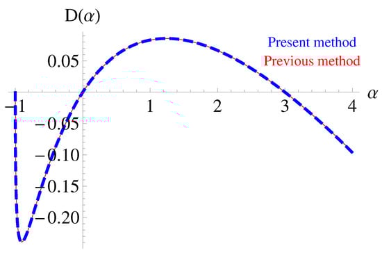
Figure 1. Numerical evaluation of the Evans function $E\left(\alpha \right)$ for the Equation (28).

We now consider $a=-1,$$b=+1$ and $n=2$ in (19), so that

$$u_t=u_{xx}-u+u^2,u_0^{{}^{″}}-u_0+u_0^2=0$$

(35)

and

$$u_0\left(x\right)=\frac{3}{2}{\mathrm{sech}}^2\left(\frac{x}{2}\right).$$

Consequently, $A_0\left(\alpha \right)$ and $A_1\left(x\right)$ become

$$A_0\left(\alpha \right)=\left(\begin{array}{cc}0& 1\\ \alpha +1& 0\end{array}\right)\mathrm{and}{A}_1\left(x\right)=\left(\begin{array}{cc}0& 0\\ -3{\mathrm{sech}}^2\left(\frac{x}{2}\right)& 0\end{array}\right),$$

(36)

respectively.

The Evans function $E\left(\alpha \right)$ is computed numerically for the Equation (35) and is shown in Figure 2. We find from Figure 2 that the Evans function $E\left(\alpha \right)$ has three discrete eigenvalues at $\alpha =-\frac{3}{4}$, $\alpha =0$ and $\alpha =\frac{5}{4}$. Since there exists a positive eigenvalue for the Evans function $E\left(\alpha \right)$ of the linearized stability problem for a pulse solution of (24), therefore, this pulse solution is unstable. It is also appropriate to compare our analytical and numerical results with the results in [1]. We can thereby see an excellent agreement between the results developed in this article and the earlier results in [1].

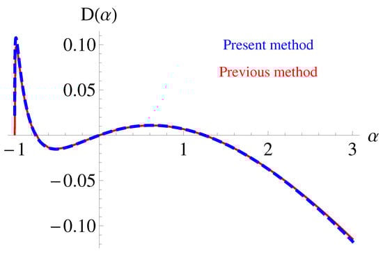
Figure 2. Numerical evaluation of the Evans function $E\left(\alpha \right)$ for the Equation (35).

4. A Direct Approach for Analyzing the Stability of Traveling Wave Solutions

Here, in this section, we present an approach for solving the Sturm-Liouville problem arising from a stability analysis for traveling waves. The idea behind this approach is inspired by some results for the Legendre functions and the Legendre polynomials (see also the recent investigations [23,24] involving applications of the substantially more general Jacobi polynomials).

The Legendre operator is given by

$$\widehat{\mathcal{L}}=\frac{d}{dx}(1-x^2)\frac{d}{dx}=(1-x^2)\frac{d^2}{d{x}^2}-2x\frac{d}{dx}.$$

We consider the following eigenvalue problem:

$$\widehat{\mathcal{L}}u=\alpha u$$

(37)

or, equivalently,

$$(1-x^2)u^{{}^{″}}-2x{u}^{{}^{\prime }}=\alpha u.$$

(38)

This equation has regular singular points at $x=\pm 1.$ However, if

$$\alpha =-n(n+1)(n=0,1,\cdots ),$$

then the solution of the Equation (37) or (38) is finite as $x\to \pm 1.$ In this case, the solution of (32) is known as a Legendre polynomial $P_n\left(x\right).$ We also note that $\alpha =0$ is an eigenvalue of the problem (38).

We now consider the associated Legendre operator

$${\widehat{\mathcal{L}}}_a=(1-x^2)\frac{d}{dx}(1-x^2)\frac{d}{dx}$$

and consider the following eigenvalue problem:

$${\widehat{\mathcal{L}}}_{a}u=\alpha u.$$

(39)

We note that $x=\pm 1$ are regular singular points of (39). The solution of (39) is finite as $x\to \pm 1$ if $\alpha =0,$ so that $\alpha =0$ is an eigenvalue of (39). In order to find the relationship between the stability analysis and the results for the Legendre functions, we consider the general example given by the Equation (19). Thus, for instance, we assume that $a<0$ and $b>0$, so that the solution $u_0\left(x\right)$ of the second equation in (19) is given by

$$u_0\left(x\right)=\alpha {\left[\mathrm{sech}\left(kx\right)\right]}^{\frac{2}{n-1}}(n>1),$$

(40)

where

$$k^2=-\frac{a{(n-1)}^2}{4}\mathrm{and}\alpha ={\left(\frac{2k^2(n+1)}{b{(n-1)}^2}\right)}^{\frac{1}{n-1}}.$$

Now, the perturbed equation for (19) is given by

$$U^{{}^{″}}-(\alpha +|a\left|\right)U+\frac{\left|a\right|n(n+1)}{2}{\mathrm{sech}}^2\left(kx\right)U=0.$$

(41)

By using the transformation $\xi =tanh\left(kx\right)$, (41) becomes

$$(1-{\xi }^2)((1-{\xi }^2)\dot{U}\dot{)}-\frac{4(\alpha +|a\left|\right)}{{\left|a\right|(n-1)}^2}U+\frac{2n(n+1)}{{(n-1)}^2}(1-{\xi }^2)U=0$$

(42)

$$\left(\dot{U}=\frac{dU}{d\xi };-1<\xi <1\right).$$

Equation (42) has two regular singular points at $\xi =\pm 1.$ In the original variable x, they correspond to $x\to \pm \in$ and are regular singular points of (19). Indeed, (42) can be written in the form:

$$(1-{\xi }^2)\ddot{U}-2\xi \dot{U}-\frac{4(\alpha +|a\left|\right)}{{\left|a\right|(n-1)}^2(1-{\xi }^2)}U+\frac{2n(n+1)}{{(n-1)}^2}U=0.$$

(43)

Equation (43) has the solution given by

$$U(\xi ,\alpha )=a_0{P}_{\beta }^{\pm \delta }\left(\xi \right),\beta =-\frac{1}{2}\pm \frac{3n+1}{2(n-1)},\delta =\frac{2}{n-1}\sqrt{\frac{\alpha +\left|a\right|}{\left|a\right|}}$$

(44)

In the Equation (44), the finite solutions require that $\beta =\frac{n+1}{n-1}$ and $\delta$ are positive integers. We search now for solutions of (44) which satisfy the following limit relationship:

$$\underset{\xi \to \pm 1}{lim}U(\xi ,\alpha )=0.$$

This condition determines the solution of the eigenvalue problem (41). We remark that this solution does not depend on the coefficient of the nonlinear term in (19), namely, b.

If $\beta =\frac{n+1}{n-1}$ is a positive integer, then we find from the properties of associated Legendre polynomials that

$$P_{\beta }^{\delta }\left(\xi \right)=0(\delta >\beta )$$

or

$$\alpha >\left|a\right|\frac{(n+3)(n-1)}{4}.$$

The finite solutions of (42) as $\xi \to \pm 1$ (or $x\to \pm \in$) are given by

$$U=a_0{P}_{\beta }^{\delta }(\delta \leqq \beta ),$$

where $\delta$ and $\beta$ are integers and $a_0$ is a constant. The required values of $\alpha$ are determined by the following equation:

$$\frac{2}{n-1}\sqrt{\frac{\alpha +\left|a\right|}{\left|a\right|}}=\delta =0,1,2,\cdots ,\frac{n+1}{n-1}.$$

(45)

Among the values of $\alpha$ which satisfy (45), we select the values which satisfy the eigenvalue condition. To make these results clear, we consider the following special cases:

(I)

If $n=3$, $a=-1$ and $b=2$, the first equation in (19) becomes the Newell-Whitehead equation. Then, from (45), we obtain $\alpha =-1,0,3$. The corresponding eigensolutions are given, respectively, by

$$U_1=a_0(3{\xi }^2-1),$$

$$U_2=a_0\xi \sqrt{1-{\xi }^2}$$

and

$$U_3=a_0(1-{\xi }^2).$$

We remark that the above results for $\alpha$ are exactly the zeros of the Evans function $E\left(\alpha \right)$ which we have found numerically (see Figure 1). But $\alpha =-1$ is not an eigenvalue as the corresponding solution

$$U_1=a_0(3{\xi }^2-1)$$

does not satisfy the eigenvalue condition. Thus, clearly, the only eigenvalues are $\alpha =0$ and $\alpha =3$, so that the solution is unstable. To examine the effects of varying the parameter a, we take $a=-4$, $n=3$ and $b=2$. We find that the values of $\alpha$ such that finite solutions as $x\to \pm \in$ exist are $\alpha =-4$ or $\alpha =9$, besides $\alpha =0$, with eigensolutions given by

$$U_1=a_0(1-3{\xi }^2),$$

$$U_2=a_0(1-{\xi }^2)$$

and

$$U_3=a_0\xi {(1-{\xi }^2)}^{\frac{1}{2}}.$$

We find again that $\alpha =-4$ is not an eigenvalue. Thus, the effect of increasing $\left|a\right|$ is that the positive eigenvalue shifts to the right on the $\alpha$-axis.

(II)

If $n=2$, $a=-1$ and $b=1$, then (19) becomes the Fisher equation.

From (45), we find that $\alpha =-1$, $-3/4$, 0, $5/4$. The corresponding eigensolutions are

$$U_1=a_0\xi (5{\xi }^2-3),$$

$$U_2=a_0{(1-{\xi }^2)}^{\frac{1}{2}}(5{\xi }^2-1),$$

$$U_3=a_0\xi (1-{\xi }^2)$$

and

$$U_4={(1-{\xi }^2)}^{\frac{3}{2}}.$$

Here, $\alpha =-1$ is again not an eigenvalue, while $\alpha =-\frac{3}{4}$, 0, $\frac{5}{4}$ are eigenvalues and they are exactly the zeros of the Evans function $E\left(\alpha \right)$ (see Figure 2). We remark that the solution of the Sturm-Liouville eigenvalue problem for (19) is too simple, because it is directly related to the associated Legendre polynomials.

We summarize these results in the following table. We fix the value $a=-1$ and b is any arbitrary positive real number.

From Table 1, we remark that the number of real eigenvalues for the Equation (41) is $(n+1)/(n-1)$. We now present an approach which may enable us to treat general problems. It is based mainly on polynomial solutions of differential equations (or truncation of the series solution).

Table 1. Special cases for the non-eigenvalue and eigenvalue which satisfied the eigenvalue condition and then it is the zeros of the Evans function $E\left(\alpha \right)$.

The Case	Values of $\mathit{\alpha }$ Where ${lim}_{\mathit{\xi }\to \pm \in }\mathit{U}(\mathit{\xi },\mathit{\alpha })$ Exists	Eigensolutions	Eigenvalues Where ${lim}_{\mathit{\xi }\to \pm \in }\mathit{U}(\mathit{\xi },\mathit{\alpha })=0$
n = 3	$-1$	$U_1=a_0{P}_2^0$	-
	0	$U_2=a_0{P}_2^1$	0
	3	$U_3=a_0{P}_2^2$	3
n = 2	$-1$	$U_1=a_0{P}_3^0$	-
	$-3/4$	$U_2=a_0{P}_3^1$	$-3/4$
	0	$U_3=a_0{P}_3^2$	0
	$5/4$	$U_4=a_0{P}_3^3$	$5/4$
n = 3/2	$-1$	$U_1=a_0{P}_5^0$	-
	$-15/16$	$U_2=a_0{P}_5^1$	$-15/16$
	$-3/4$	$U_3=a_0{P}_5^2$	$-3/4$
	$-7/10$	$U_4=a_0{P}_5^3$	-
	0	$U_5=a_0{P}_5^4$	0
	$9/16$	$U_6=a_0{P}_5^5$	$9/16$

We should remark that, in order to obtain the solution of (43) in the form of the associated Legendre polynomials, the solution expansion is taken near the regular point $\xi =0$. In what follows, the solution expansions are taken near a regular singular point at either plus or minus infinity ($x=\pm \in$). In the Equation (40), we assume that $\mathrm{sech}\left(kx\right)=\gamma$, so that it becomes

$${\gamma }^2(1-{\gamma }^2)\ddot{U}+\gamma (1-2{\gamma }^2)\dot{U}-\frac{4(\alpha +|a\left|\right)}{{\left|a\right|(n-1)}^2}U+\frac{2n(n+1)}{{(n-2)}^2}{\gamma }^{2}U=0(0<\gamma <1).$$

(46)

In connection with the Equation (46), we remark that $\gamma =0,\pm 1$ are regular singular points and $\gamma =0$ corresponds to $x\to \pm \in$, which are regular singular points. We search for solutions of (46) in the form of

$$U=\sum _{m=0}^{\in }{a}_n{\gamma }^{m+d}.$$

The indicial equation gives rise to

$$d=\pm \frac{2}{n-1}\sqrt{\frac{\alpha +\left|a\right|}{\left|a\right|}}.$$

Here $a_0$ is arbitrary, while $a_1=0$. In order to obtain finite solutions, we take the upper sign in the last equation for d. The general recursion formula is given by

$$\begin{array}{cc}\hfill & \left[{(m+d)}^2-\frac{4(\alpha +|a\left|\right)}{{\left|a\right|(n-1)}^2}\right]a_m\hfill \\ \hfill & -\left[(m+d-1)(m+d-2)-\frac{2n(n+1)}{{(n-1)}^2}\right]a_{m-2}=0(m\geqq 2),\hfill \end{array}$$

(47)

where

$$d=\frac{2}{(n-1)}\sqrt{\frac{\alpha +\left|a\right|}{\left|a\right|}}(\alpha >-|a\left|\right).$$

Equation (47) admits a polynomial solution if there exists an integer $m\geqq 2$ and $d>0$ such that the coefficient of $a_{m-2}$ vanishes. This holds true for

$$d+m=\frac{3n-1}{n-1}.$$

(48)

Certainly, when analyzing the Equation (47) by taking

$$m=2,4,\cdots \mathrm{and}2k<\frac{3n-1}{n-1},$$

we find the same results as before. So, instead, we can find results from (47) and (48).

In view of (47), we have a lower bound for $\alpha$ and from (47) we obtain the least upper bound for $\alpha$ (or the dominant value of $\alpha$), namely, ${\alpha }_0$ when $m=2$. This is true because, for $m>2$, the values of d decrease, and then $\alpha$ decreases. In fact, when $m=2$, we obtain

$${\alpha }_0=\left|a\right|\frac{(n+3)(n-1)}{4}$$

and the following result holds true:

$$-\left|a\right|<\alpha \leqq \left|a\right|\frac{(n+3)(n-1)}{4}.$$

(49)

The last result suggests the introduction of the following general localization concepts of eigenvalues of the Sturm-Liouville problem.

We now define what is meant by a dominant eigenvalue and a dominant solution. A dominant eigenvalue ${\alpha }_0$ is the least upper bound of the eigenvalues $\alpha \leqq {\alpha }_0$. A dominant solution is a solution which corresponds to a dominant eigenvalue ${\alpha }_0$. In the solution expansion near a regular singular point, we conjecture that a dominant solution is obtained at the lowest-order truncation of the series, namely, at $m=2$. Consequently, the dominant eigenvalue is determined by the solution of the recursion formulas for $m\geqq 2$. We return to (47) in order to check that we get the same results found previously. To this end, we reconsider the same examples.

For $n=3$, $a=-1$ and $b=2$, we find that (48) gives

$$m=4-\sqrt{1+\alpha }\geqq 2.$$

For $m=2$ and $m=4,$ we have $\alpha =3$ and $\alpha =-1$, respectively. For $n=2$, $a=-1$ and $b=1$, (48) gives rise to

$$m=5-2\sqrt{1+\alpha }\geqq 2.$$

Thus, we obtain $\alpha =-\frac{3}{4}$, $\frac{5}{4}$ for $m=2,4$, respectively. The corresponding eigensolution can be obtained as well.

We remark that we have obtained the same results as above. On the other hand, polynomial solutions found through an expansion near a regular singular point gives rise to values of $\alpha \ne 0$. We mention that, when analyzing the stability of pulse solutions of the first equation in (19) when $a>0$ and $b<0$, we find that the eigenvalues are non-positive. These solutions are then stable.

5. Conclusions

In our present investigation, we have studied the stability analyses of traveling wave solutions (pulses) for a single reaction-diffusion equation. This stability has been studied here by using the Evans function $E\left(\alpha \right)$ and a direct approach. We have successfully recovered the results which are known in the literature on the stability of solutions of a single reaction-diffusion equation. The numerical results presented in this article have been computed with the aid of Mathematica.

In view of the recent investigations on traveling waves, using fractional-order derivatives (see, for example, [25,26,27]), which have successfully accomplished important advancements on the subject, it is believed that these interesting situations can be treated adequately by the approach presented in this article. Thus, remarkably, this work is capable of further motivating and advancing researches on the subject dealt with in our present investigation. Moreover, in several other fields involving wide-spread applications of various families of fractional-order derivatives in the study of the reaction-diffusion and other important equations of the mathematical and physical sciences, this article may lead to the modeling and analysis of such interesting phenomena as the distributed time-delay, the behavior of solutions in transition states, and so on. All such developments are significantly meritorious and potentially useful in the engineering sciences as well (see also the related recent works [28,29,30]).

References

- Saad, K.M.; El-Shrae, A.M. Numerical methods for computing the Evans function. ANZIAM J. 2011, 77, E76–E99. [Google Scholar] [CrossRef]
- Pego, R.L.; Weinstein, M.I. Eigenvalues and instabilities of solitary waves. Philos. Trans. R. Soc. Lond. Ser. A Math. Phys. Engrg. Sci. 1992, 340, 47–94. [Google Scholar]
- Kapitula, T. Stability analysis of pulses via the Evans function: Dissipative systems. In Dissipative Solitons; Akhmediev, N., Ankiewicz, A., Eds.; Lecture Notes in Physics; Springer: Berlin/Heidelberg, Germany; New York, NY, USA, 2005; Volume 661, pp. 407–428. [Google Scholar]
- Kapitula, T.; Sandstede, B. Stability of bright solitary wave solutions to perturbed nonlinear Schrödinger equations. Phys. D Nonlinear Phinomen. 1998, 124, 58–103. [Google Scholar] [CrossRef]
- Evans, J.W. Nerve Axon equations. I: Linear approximations. Indiana Univ. Math. J. 1972, 21, 877–955. [Google Scholar] [CrossRef]
- Evans, J.W. Nerve Axon equations. III: Stability of the nerve impulses. Indiana Univ. Math. J. 1972, 22, 577–594. [Google Scholar] [CrossRef]
- Evans, J.W. Nerve Axon equations. IV: The stable and unstable impulse. Indiana Univ. Math. J. 1975, 24, 1169–1190. [Google Scholar] [CrossRef]
- Jones, C.K.R.T. Stability of the travelling wave solutions of the Fitzhugh-Nagumo system. Trans. Am. Math. Soc. 1984, 286, 431–469. [Google Scholar] [CrossRef]
- Alexander, J.C.; Gardner, R.A.; Jones, C.K.R.T. A topological invariant arising in the stability analysis of travelling waves. J. Reine Angew. Math. 1990, 410, 167–212. [Google Scholar]
- Henry, D. Geometric Theory of Semilinear Parabolic Equations; Springer: Berlin/Heidelberg, Germany; New York, NY, USA, 1981. [Google Scholar]
- Gardner, R.A.; Jones, C.K.R.T. Traveling waves of a perturbed diffusion equation arising in a phase field model. Indiana Univ. Math. J. 1990, 39, 1197–1222. [Google Scholar] [CrossRef]
- Aparicio, N.D.; Malham, S.J.A.; Oliver, M. Numerical evaluation of the Evans function by Magnus integration. BIT Numer. Math. 2005, 45, 219–258. [Google Scholar] [CrossRef]
- Gubernov, V.; Mercer, G.N.; Sidhu, H.S.; Weber, R.O. Evans function stability of combustion waves. SIAM J. Appl. Math. 2003, 63, 1259–1275. [Google Scholar]
- Gubernov, V.; Mercer, G.N.; Sidhu, H.S.; Weber, R.O. Numerical methods for the travelling wave solutions in reaction-diffusion equations. ANZIAM J. 2002, 44, 271–289. [Google Scholar] [CrossRef][Green Version]
- Malham, S.; Niesen, J. Evaluating the Evans function: Order reduction in numerical methods. Math. Comput. 2008, 77, 159–179. [Google Scholar] [CrossRef]
- Simon, P.L. On the structure of spectra of travelling waves electron. J. Qual. Theory Differ. Equ. 2003, 15, 1–19. [Google Scholar]
- Bridges, T.J. The Orr-Sommerfeld equation on a manifold. Proc. R. Soc. Lond. A Math. Phys. Engrg. Sci. 1999, 455, 3019–3040. [Google Scholar] [CrossRef]
- Afendikov, A.L.; Bridges, T.J. Instability of the Hocking-Stewartson pulse and its implications for three-dimentional Poiseuille flow. Proc. R. Soc. Lond. A Math. Phys. Engrg. Sci. 2000, 457, 3019–3040. [Google Scholar]
- Allen, L.; Bridges, T.J. Numerical exterior algebra and the compound matrix method. Numer. Math. 2002, 92, 197–232. [Google Scholar] [CrossRef]
- Sattinger, D.H. On the stability of waves of nonlinear parabolic systems. Adv. Math. 1976, 22, 312–355. [Google Scholar] [CrossRef]
- Fiedler, B.; Scheel, A. Spatio-temporal dynamics of reaction-diffusion patterns. In Trends in Nonlinear Analysis; Kirkilionis, M., Krömker, S., Rannacher, R., Tomi, F., Eds.; Springer: Berlin/Heidelberg, Germany; New York, NY, USA, 2003; pp. 23–152. [Google Scholar]
- Sandstede, B.; Scheel, A. On the structure of spectra of modulated travelling waves. Math. Nachr. 2001, 232, 39–93. [Google Scholar] [CrossRef]
- Singh, H.; Pandey, R.K.; Srivastava, H.M. Jacobi collocation method for the approximate solution of some fractional-order Riccati differential equations with variable coefficients. Phys. A Statist. Mech. Appl. 2019, 523, 1130–1149. [Google Scholar] [CrossRef]
- Singh, H.; Pandey, R.K.; Srivastava, H.M. Solving non-linear fractional variational problems using Jacobi polynomials. Mathematics 2019, 7, 224. [Google Scholar] [CrossRef]
- Gao, F.; Yang, X.-J.; Srivastava, H.M. Exact travelling-wave solutions for linear and non-linear heat transfer equations. Therm. Sci. 2017, 21, 2307–2311. [Google Scholar] [CrossRef]
- Yang, X.-J.; Gao, F.; Srivastava, H.M. Exact travelling wave equations for the local fractional two-dimensional. Burgers-type equations. Comput. Math. Appl. 2017, 73, 203–210. [Google Scholar] [CrossRef]
- Srivastava, H.M.; Günerhan, H.; Ghanbari, B. Exact traveling wave solutions for resonance nonlinear Schrödinger equation with intermodal dispersions and the Kerr law nonlinearity. Math. Methods Appl. Sci. 2019, 42, 7210–7221. [Google Scholar] [CrossRef]
- Srivastava, H.M.; Saad, K.M. Some new models of the time-fractional gas dynamics equation. Adv. Math. Models Appl. 2018, 3, 5–17. [Google Scholar]
- Srivastava, H.M.; Saad, K.M. New approximate solution of the time-fractional Nagumo equation involving fractional integrals without singular kernel. Appl. Math. Inf. Sci. 2020, 14, 1–8. [Google Scholar]
- Srivastava, H.M.; Saad, K.M.; Al-Sharif, E.H.F. New analysis of the time-fractional and space-time fractional-order Nagumo equation. J. Inf. Math. Sci. 2018, 10, 545–561. [Google Scholar]
© 2020 by the authors. Licensee MDPI, Basel, Switzerland. This article is an open access article distributed under the terms and conditions of the Creative Commons Attribution (CC BY) license (http://creativecommons.org/licenses/by/4.0/).