Abstract
Due to the lack of reliable methods, manual fish counting is popular on farms. However, this approach is time and labor intensive. Using an echosounder and the echo-integration technique could be a better alternative. The echo-integration method has been widely used in fish abundance estimation in waterbodies because of its simplicity. However, most of the research is concentrated on the open ocean, whereas fish count estimation in farming cages has not been explored much. Using the echo-integration method in a cage offers its own unique sets of problems. Firstly, the echo signal reflected from the cage boundaries should also be taken into account. Secondly, the fish inside a cage behave differently with time, as their mobility pattern is highly dependent on sunlight and water current. In this paper, fish behavior inside an offshore cage over time was extensively studied, and based on that a real-time fish counter system using a commercial echosounder was developed. The experiments demonstrate that our method is simple, user-friendly, and has an estimation error of less than 10%. Since our method accurately estimated fish abundance, the method should be reliable when making fish management decisions.
1. Introduction
In fish farming, knowing the exact amount of fish in a cage is of paramount importance, as it helps to provide the best conditions for the fish under cultivation, thereby guaranteeing the health and growth of the species [1,2,3,4]. As the fish food and other resources are expensive, the knowledge of the fish individuals is necessary for the optimum utilization of these [3,4]. However, there is no easy and reliable method to keep track of the exact number of fish in a cage, and hence the farmer has to use an intelligent guess out of experience or do manual counting for fish management. Furthermore, no practical solution is available that can be used by third-party companies, such as insurance companies, to verify the fish count claimed by farmers [5]. Therefore, a portable device or a method that gives an accurate estimation of fish count in a cage is highly desirable.
Over the years, various techniques and methods have been widely used and proposed for the fish counting problem. For instance, the acoustics echo-sounding method, the machine vision-based method, the environmental DNA-based method, and the resistivity counter-based method are some popular methods that have been used in fish counting [6]. Among these, the acoustic echo-sounding method is one of the most popular methods to estimate fish abundance because of simplicity and noninvasive nature [7]. In this technique, echosounder sends an acoustic ping and the reflected echoes from fish are analyzed to estimate fish abundance. The key idea relies on the detection of reflected energy produced by the target as the amount of energy is proportional to the number of targets. The scientific use of acoustics for counting fish has been widespread over the last three decades [8,9,10,11,12,13,14,15,16,17,18,19,20,21]. Modern echosounder and echo processing software implement the echo-integration technique to study fish and their behavior [12,13,14,15,16,17]. Even though echo-integration has been widely used in the open sea, when used in a cage, it offers a unique set of challenges [18,19,20,21]. For instance, the reverberation in the cage due to the echoes of the acoustical signal from the boundaries needs to be taken into account when performing echo integration [19,22]. Therefore, some techniques should be used to remove the cage-boundary signal from the received signal, as discussed in [5]. Another issue that must be taken into account is the behavior of fish in a cage [23]. The accuracy of echo-integration is dependent on the transducer’s ability to capture the fish distribution in a cage. Thus, the knowledge of how fish behave and move in a cage at a particular time is salient for accurate estimation. Another problem in fish-abundance estimation by acoustics is the shadowing effect, which can seriously affect the fish count results when dense aggregations of fish are encountered. Compensation for the attenuation of the echo strength due to the shadowing effect is necessary [24]. However, in the case of low fish density and random movement, the shadowing effect is minimum [24].
The main objective of this research is to investigate the possibility of using a commercial echosounder for fish counting in real time. The aim is to develop a practical, portable, and reliable system to estimate fish numbers in offshore farming cages. For that, firstly, we studied the behavior of fish in a net cage by monitoring continuously for two months using an echosounder and an underwater camera. Based on the observation and analysis, an algorithm and the manual for experimentation were developed. The experimental results verify that when fish counting is performed under the defined guidelines, the estimation accuracy of the proposed algorithm is high. The finding of this research could be beneficial to the researchers and the professionals working in fish management, especially in offshore fish farming.
2. Proposed Fish Counting Algorithm
This section details the fish count algorithm used in the paper. The algorithm employs the echo-integration technique to count fish in a cage. The algorithm was designed under the assumption that the cage under investigation contains fish of the same species only, but potentially of variable length, which is generally the case in fish farming cages. The basic idea of the algorithm is to estimate the fish count based on the population density (per m) of a cage, which is calculated by scaling (measured by echosounder) with the average target strength (TS) (measured by sampling) of fish in the cage. Therefore, the more fish are uniformly distributed in a cage, the higher the accuracy of the algorithm. The algorithm assumes low fish density and sufficiently random distribution; thus, the shadowing effect is not considered.
2.1. Theoretical Background
The fundamental principle that is used in the algorithm is explained here.
2.1.1. Target Strength
Target strength (TS) is a measure of the proportion of the incident energy which is backscattered by the target. TS is used as a scaling factor in biomass estimation [11,25]. TS is expressed in decibels and is given by
where is acoustic backscattering cross-section reflected by a target.
2.1.2. Backscattering Coefficient
When the individual targets are very small and there are many in the sampled volume, their echoes combine to form a integrated received signal. However, the echo intensity is still a measure of the biomass in the water column. The basic acoustic measurement is the volume backscattering coefficient, , given by
where V is the sampled volume occupied by a scattering medium or multiple discrete targets. Similarly, area backscattering coefficient, , is a measure of the energy returned from a layer between two depths and in the water column. It is defined as the integral of with respect to depth through the layer and is given by
2.1.3. Fish Count Estimation
Theoretically, fish density is obtained by diving by . However, there can be multiple targets of different sizes and spices in a water body. Therefore, the mean acoustic backscattering cross section of targets denoted by is used. The target density, , expressed as the number of fish per unit surface area is given by
Finally, the fish count, N, within an area of A can be calculated as,
Note that N is the estimation for a layer or a water column only. To estimate fish for a depth range, a summation of estimation of all the layers between the range is required.
2.2. Algorithm
This section explains how the above theory is used in the algorithm. For each echo ping sent, a typical echosounder provides data measured at each water column (layer) of z m height between the sampled range interval m and m measured from the top, where is closer to the surface. The algorithm assumes that is larger than the cage bottom. The algorithm takes data as an input. Additionally, the algorithm requires length frequency key and cage backscattering strength as inputs, which are explained below.
2.2.1. Length Frequency Key
The average TS of fish in a cage can be estimated by sampling some fish. To calculate <TS> from the sampled fish, the algorithm takes length frequency key (LFK) as an input. LFK is a table of two columns that records the number of fish of particular length, as shown in Table 1. Note that the length in the table is the total length of fish round up to a nearest cm.

Table 1.
Length frequency key of fish samples from Cage1.
2.2.2. Cage Backscattering Strength
The echosounder data collected from a cage also contain the signal reflected from the cage. A method needs to be devised to remove the net signal from the received signal. Here, we simply subtract the expected cage signal from the received signal. For that, data need to be measured under an empty cage condition (cage without a fish). Given the empty cage data, the accumulated back-scattering coefficient of the empty net, , for a ping, is calculated as follows:
where is of the empty net at r m. Note that the value of must be larger than the cage bottom such that the overall net bottom signal is fully considered.
2.2.3. Fish Counting
Along with data, the algorithm takes , , fish species, (mean ), and LFK as inputs and returns the fish count as the output. At first, based on the LFK table provided, the algorithm calculates . The TS of a fish is well defined in the form as follows:
where A and B are the standard coefficients for a fish species and L is the length of the fish. The TS of commonly farmed fish in Korea is shown in Table 2, which is maintained as a lookup table by the algorithm. Assuming n denotes the number of rows in LFK table, denotes the number of fish with length L, is calculated as follows:
where,
Table 2.
Target strength (TS) at 200 KHz of some common fish farmed in Korea.
The next step of the algorithm is to sum all the values of a ping between and . The algorithm reads data of a ping at a time, and calculates accumulated back-scattering coefficient, , as follows,
The is the accumulated back-scattering coefficient over the sampled range; therefore, it contains the information about fish abundance in the entire range. However, it also contains the signal from the cage. Assuming no echo from the sidewalls, one possible way to remove the net signal is to select just above the net bottom. However, there are two problems with this approach: (i) the net bottom level changes with sea current; therefore, using a fixed value is not suitable and (ii) even if the net bottom is stationary, some signal from the fish exactly at the net bottom will be discarded because of the range resolution of the echosounder. In this study, an alternative approach is employed. The average net signal is subtracted from the total signal using the following equation:
Finally, the amount of fish () per ping is estimated as follows:
where A is the surface area of the net. Since by is the number of fish per m, multiplying it with the surface area gives the total number of fish in the cage. The process continues to the next ping and the average fish count over pings is calculated by taking the moving average of . We note that the algorithm assumes the uniform distribution of fish in the cage in the form of a parallelepiped.
2.3. Fishcounter Software
The final Fishcounter software that implements the above algorithm which acquired data from the Simrad echosounder was developed using C++ Builder [29]. All the necessary input parameters required for the algorithm are provided via the graphical user interface. The software is designed to read raw data directly from the echosounder in real time; therefore, it should operate simultaneously on the same PC running EK15 software. The software has provision to record by performing echo reading over an empty cage. At the end of the reading, pressing the “Empty Cage” button saves under the supplied variable name. During operation, EK15 software reads data from the echosounder and simultaneously writes on the defined port number. Fishcounter reads data from the port, processes it, and displays the result. A screenshot of Fishcounter software displaying the fish count result from an experiment performed in Cage1 is shown in Figure 1. Along with the estimated fish count, the software also displays standard deviation (SD), the minimum count, and the maximum possible count in the cage. With the help of the software, the fish count in a cage can be estimated in real time.
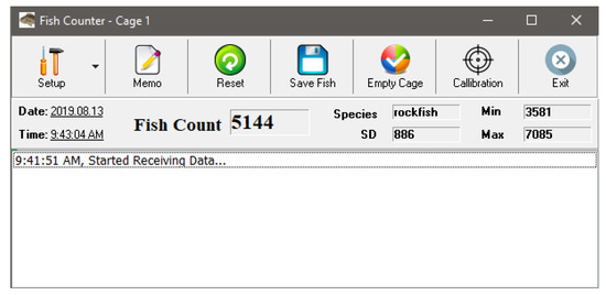
Figure 1.
Screenshot of Fishcounter software displaying results from one of the experiments in Cage1.
3. Materials and Methods
3.1. Study Area
The experiments were performed on a commercial offshore fish farm located in Wando, Korea. The farm consists of more than 50 individual cages made on a floating grid each nylon net cage having dimensions of 7 × 7 × 7 m with an 11 mm square mesh. Note that even though the actual cage height is 7 m, about 0.5 m of the cage is above the water surface, as can be seen in Figure 2. Three cages (named Cage1, Cage2, and Cage3 for ease of referencing) were found to be suitable for our experimental purposes based on their accessibility, the target length, and fish count, and their details are listed in Table 3. Cage1 and Cage3 consist of Roshfish, whereas Cage3 consists of black porgy. A total of 35 fish were sampled from each cage and recorded in their respective LFK tables. The maximum and minimum sampled fish length (total length) and the total fish count for each cage are illustrated in Table 3. At the time of the experiment, the fish in all three cages were two years old. The total count shown in the table was obtained from the farm’s records.
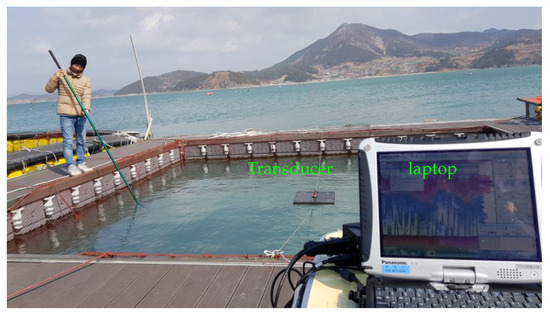
Figure 2.
An experiment performed on a cage using Simrad EK15.
Table 3.
Details of all the three fish cages used in the experiments.
3.2. Data Acquisition
In all the experiments, Simrad EK15 echosounder and a single down-looking transducer were used [30]. The echosounder comes with a transducer, a processing unit, and PC software. The echosounder operates at 200 KHz with a 26 beam width. The transducer was mounted on a floating panel; therefore, is not free from turbulence due to water current. The transducer was always placed at the center of a cage, as illustrated in Figure 2. The transducer sends a ping at regular interval and the received echo is recorded by Simard EK15 software in a “.raw” file. Note that Simrad EK15 records the at each water column in a dB scale, as illustrated by the following equation:
In the proposed algorithm, denotes the implicit conversion of read from the echosounder. Simard EK15 software can also be configured to simultaneously write recorded on a certain Ethernet port. This feature was used to develop our fish counting software.
3.3. Experiments Performed
Mainly four types of experiments were carried out: (i) empty net analysis, (ii) long-term experiments, (iii) net bottom analysis, and (iv) short experiments. In all the experiments, = 1 m and = 7 m were used.
The empty net analysis was performed to estimate . Using the settings from Table 4, in total, 5 sets of the experiment were performed over an empty net cage, each lasting for more than 30 min. The mean was then calculated. We note that the experiment was performed on a separate cage but had the same age and material as Cage1, Cage2, and Cage3. The same was used for net subtraction by the fish counting algorithm for all experiments.
Table 4.
Echosounder parameters used during data collection of short experiments.
The long-term experiments were performed between the period of 6th September 2019 and 25th October 2019 to study the behavior of fish in the cage over time. A total of four sets of long-term experiments were performed on Cage1, each lasting for 4 or 5 days. The echosounder was operated using the setting from Table 5. To minimize the turbulence, experiments were performed starting from a day with minimal current and the echosounder data were collected continuously for the next 3–4 days; the tidal information was obtained from [31]. The data collection on the remote computer at the experimental site was closely monitored and managed regularly from the lab using remote access software (Chrome Remote Desktop [32]). To illustrate the observation from the long-term experiments, an analysis conducted from a representative experiment of 4 days (92 h to be exact) was demonstrated. We note that the experiment was chosen randomly for the purpose of demonstration only, but the pattern was found to be similar for all the experiments.
Table 5.
Echosounder parameters used during data collection of long-term experiments.
The results from the long-term experiments suggest that fish count is affected by the position of the net bottom. Therefore, the net bottom analysis was performed to confirm it. The settings from Table 4 were used. Two experiments were performed: one on 2019.08.08 on a low current day and the other on 2019.08.14 on a high current day. Additionally, during the experiment on the low-current day, the cage was intentionally pulled up two times to see how it affected the fish count.
The experimental results suggested that the accuracy of the proposed algorithm is the highest during dark hours of the lowest current day at the slack water time. To confirm it, a total of 15 short experiments were performed, satisfying the fore-mentioned conditions on all the three cages listed in Table 3. The experiments were performed from the lowest current day 2019.09.07 to 2019.09.09, for three days, in the evening during slack water [31]. The device settings are shown in Table 4. To save device setting time, each day a total of 5 sets of experiments, each of 5–10 min were repeated on a single cage only.
3.4. Data Analysis
The raw files were analyzed using Echoview 10 [33], Octave script (Octave 5.1.0), and our home-brew echogram viewer software. Echoview and home-brew software were used to visualize the echogram and analyze the TS and SV values. Echogram along with the captured videos were used to study fish behavior and movement over time.
In the case of long term data, fish counting was performed using Octave [34]. The fish counting algorithm was implemented in Octave that takes a “.raw” file as the input and returns the fish count per ping in a from of a row matrix. The running average of the matrix was calculated to see how the fish count changes over time.
Similarly, in the case of short experiments, Fishcounter software (from Figure 1) was used for counting fish. At the end of an experiment, the fish count displayed by the software was recorded.
4. Experimental Results and Discussion
The echogram of the representative long-term experiment of 92 h is shown in Figure 3. In the figure, the region above the black horizontal line is from the cage, while the bottom half is from the sea bed. The color map is displayed at the right of the figure. The red pixel represents a strong signal from a target such as fish or the sea bed. For the ease of referencing, the first four cycles of days and nights are labeled in the figure. The red sinusoidal graph in the figure represents the change in water level over time. The maximum and the minimum water level measured were 10.6 and 7.5 m, respectively. One interesting pattern that can be observed in the echogram is that the fish tend to stay at the bottom of the net during the day and start to move upward in the evening. Similarly, after sunrise, the fish again move to the bottom. The echogram suggests minimum fish activity during the day, evidenced by the cluster of red pixels at the bottom and mostly blue and white pixels above 3 m. However, at night, the entire cage is full of red pixels, representing high fish activity. Similar mobility patterns for rockfish and other fish species have been reported [35,36,37,38].
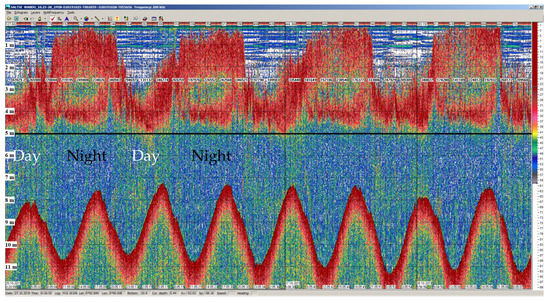
Figure 3.
Echogram for the duration of 92 h performed in Cage1.
The results of fish count performed on the above long-term experiment are demonstrated in Figure 4 and Figure 5. Since there is a clear difference in the echogram during days and at nights, the fish counts are separately shown. The data from 6 am to 6 pm are considered as the day time and the rest as the night. An echogram and its corresponding fish count result are stacked on top of each other, and their x-axes are aligned to time. The window size of 30 min (30 pings) was used to calculate the moving average of the fish count and is shown in the blue graphs. Similarly, the true fish count is shown by the dashed red lines.
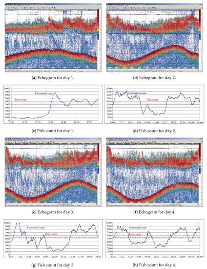
Figure 4.
Echogram and fish estimation during day time from the 92 h experiment performed in Cage1.
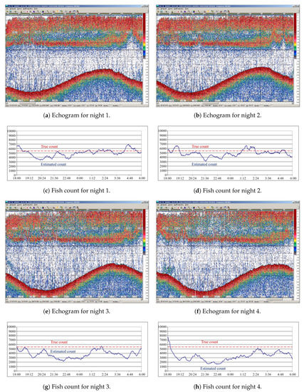
Figure 5.
Echogram and fish estimation at night time from the 92 h experiment performed in Cage1.
Figure 4 demonstrates echograms and fish counts for day times. As can be seen from the figures, the fish count varies sharply over time. The volatility of data is related to the spatiotemporal variability of the distribution of fish in the cage at different times of the day. However, some pattern in fish count was observed related to the level of illumination and tidal phenomena. The fish count results illustrate that during slack tides (at high or low tides), which correspond to peaks and valleys of the sea bed in the echograms, the estimation is significantly high, whereas at other times the count is significantly low. The reason that fish count sharply decreases during high water current is because the fish move away from the transducer beam region toward the side of the cage wall blown out by the current, which is evidenced by the echogram, as the thickness of the red pixels in the cage is notably thin compared to slack tides. Since the center of fish concentration is shifted from the center of the cage to sides, the estimation is low. Similarly, the reason for relatively high estimation of fish count during slack tides is because during these periods the current inside the cage is low and fish tend to move toward the center of the cage, forming a school, as reported in [35,36,38]. Since all or part of the school is under the transducer beam, the estimation is high.
On the other hand, the fish counts at nights are different from those during the day. As can be seen in Figure 5, at night, the estimated fish count tends to stay near to the true value and the fluctuation was significantly lower compared to that in day time. Even though the fish count gradually decreases as we move from night 1 to night 4, the estimation was consistent for a particular night. We note that a similar pattern was observed in other long term experiments also. The reason for the consistent result is that during the dark hours, due to lack of visibility, the fish move on their own without forming any school. This behavior results in uniform distribution of fish inside the cage, thereby giving consistent and stable estimation. One interesting pattern observed is that the fish count is the most accurate during slack water. The reason for relatively high accuracy is because at the slack tide the walls of the cage are relatively even, and the fish are uniformly distributed in the cage. Another noticeable observation of fish count variability between nights is that the average estimation decreases slightly as we move from the first night to the last night. Since the data collection started from the lowest current day, as time progressed, the water current increased day by day, resulting in higher turbulence on the floating transducer. This is the main reason for the decrease in the fish estimation, as evidenced by the decrease in the received signal strength.
The result from the net bottom analysis experiment is shown in Figure 6. The echograms and their corresponding fish counts are stacked over each other, and their x-axes are aligned. In Figure 6c,d, the pink graph represents fish count per ping and the red dash line denotes the true count. On the left echogram, it can be seen that the cage bottom is flat, which corresponds to absence or weak current. The echogram showed that the net bottom was stable at 6.5 m. The corresponding fish count results are also comparatively stable. The two spikes in the fish count are the result of cage pulling. The times of spikes exactly match with the times of the cage pulling. Figure 6b illustrates a high movement of cage bottom during high water current. The cage bottom fluctuated between 4.5 and 5.5 m most of the time and in only some instances attended its true depth at 6.5 m. The cage wall was also observed to be deformed washed toward the direction of current, resembling a parallelogram (side view). The sharp changes in fish counts verify that the fish count is affected by the position of the cage bottom. The highly volatile fish count graph suggests that fish counting is not suitable during a high current.
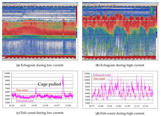
Figure 6.
Echogram and fish estimation from the net bottom analysis experiment.
The fish count result from the short experiments is shown in Table 6. The table shows that the fish count estimation of the algorithm has a maximum error of ±9.5%. Even though the number of experiments performed was limited, the results matched well with our established findings. Accuracy of echo-integration can be affected by TS estimates, TS used for scaling, fish behavior, spatial sampling error, and analysis techniques and parameters used among other factors [23]. However, the results suggest that the proposed algorithm estimates fish abundance in an offshore cage with high accuracy if experiments are performed at night during slack water on the lowest current day.
Table 6.
Estimated fish count and the error (%) of all the three cages calculated from the performed short experiments.
5. Future Work
There are still some research questions and possible future directions. Firstly, since a floating panel was used to mount the transducer, the feasibility and efficacy of using gimbals are worth investigating. Secondly, since in all the experiments a single transducer was used for the cage size of 7 × 7 × 7 m, the maximum coverage area by a single transducer could be another research direction. Thirdly, since the experiments were performed on rockfish and black porgy only, more experiments could be carried out with different fish species.
Furthermore, working on techniques to improve accuracy for day time is another future direction. For instance, covering the cage with the black curtain from all possible directions could be a way to improve accuracy. The degree of efficiency of using the black curtain during the day is required to be clarified by experiments with a controlled level of illumination in the cage. Another approach to improve accuracy is to consider the school shape in the algorithm. Since the fish move in a school during the day and when the school is directly under the transducer, the algorithm overestimates the number because the algorithm assumes the shape of a cage as a parallelepiped. The estimates can be improved if an elliptical shape is used in the calculation. This could be another future topic.
6. Conclusions
This work proposes a method to estimates fish abundance in offshore fish farming cages using an off-the-shelf echosounder. Long-term monitoring of fish in a farming cage was performed using an echosounder and the echograms were extensively analyzed. Based on the observation and the interpretation, a fish counting algorithm along with a manual was proposed. The experimental results demonstrate that the proposed method can achieve an estimation accuracy of more than 90%. Our method could be used to take fish management decisions on farms.
Author Contributions
Conceptualization, P.S., and K.K.; methodology, P.S., and M.K.; software, P.S.; validation, P.S., and M.K.; formal analysis, P.S., and K.K.; investigation, P.S., and M.K.; resources, P.S., and M.K.; data curation, P.S., and M.K.; writing—original draft preparation, P.S.; writing—review and editing, P.S.; visualization, P.S.; supervision, K.K.; project administration, K.K.; funding acquisition, K.K. All authors have read and agreed to the published version of the manuscript.
Funding
This research was a part of the project titled “Development of Automatic Identification Monitoring System for Fishing Gears”, funded by the Ministry of Oceans and Fisheries, Korea.
Conflicts of Interest
The authors declare no conflict of interest.
References
- Hernández-Ontiveros, J.M.; Inzunza-González, E.; García-Guerrero, E.E.; López-Bonilla, O.R.; Infante-Prieto, S.O.; Cárdenas-Valdez, J.R.; Tlelo-Cuautle, E. Development and implementation of a fish counter by using an embedded system. Comput. Miscs Agric. 2018, 145, 53–62. [Google Scholar] [CrossRef]
- Zheng, X.; Zhang, Y. A fish population counting method using fuzzy artificial neural network. In 2010 IEEE International Conference on Progress in Informatics and Computing; IEEE: Shanghai, China, 2010; Volume 1, pp. 225–228. [Google Scholar]
- Bacher, K.; Gordoa, A.; Sagué, O. Feeding activity strongly affects the variability of wild fish aggregations within fish farms: A sea bream farm as a case study. Aquac. Res. 2015, 46, 552–564. [Google Scholar] [CrossRef]
- Zhou, C.; Xu, D.; Lin, K.; Sun, C.; Yang, X. Intelligent feeding control methods in aquaculture with an emphasis on fish: A review. Rev. Aquac. 2018, 10, 975–993. [Google Scholar] [CrossRef]
- Sthapit, P.; Teekaraman, Y.; MinSeok, K.; Kim, K. Algorithm to Estimation Fish Population using Echosounder in Fish Farming Net. In Proceedings of the 2019 International Conference on Information and Communication Technology Convergence (ICTC), Jeju Island, Korea, 16–18 October 2019; pp. 587–590. [Google Scholar]
- Li, D.; Hao, Y.; Duan, Y. Nonintrusive methods for biomass estimation in aquaculture with emphasis on fish: A review. Rev. Aquac. 2019. [Google Scholar] [CrossRef]
- Mitson, R.B. Fisheries Sonar; Fishing News Books Ltd.: Farnham, UK, 1983. [Google Scholar]
- Thorne, R.E. An empirical evaluation of the duration-in-beam technique for hydroacoustic estimation. Can. J. Fish. Aquat. Sci. 1988, 45, 1244–1248. [Google Scholar] [CrossRef]
- Ricker, W.E. Linear regressions in fishery research. J. Fish. Board Can. 1973, 30, 409–434. [Google Scholar] [CrossRef]
- Sawada, K.; Furusawa, M.; Williamson, N.J. Conditions for the precise measurement of fish target strength in situ. J. Mar. Acoust. Soc. Jpn. 1993, 20, 73–79. [Google Scholar] [CrossRef]
- Simmonds, J.; MacLennan, D. Fisheries Acoustics: Theory and Practice, Second Edition; Blackwell Publishing Ltd.: Oxford, UK, 2005. [Google Scholar]
- Thorne, R.E. Investigations into the relation between integrated echo voltage and fish density. J. Fish. Board Can. 1971, 28, 1269–1273. [Google Scholar] [CrossRef]
- Røttingen, I. On the relation between echo intensity and fish density. Fisk. Havforskningsinstitutt. 1976, 9, 301–314. [Google Scholar]
- Misund, O.A.; Aglen, A.; Frønæs, E. Mapping the shape, size, and density of fish schools by echo integration and a high-resolution sonar. ICES J. Mar. Sci. 1995, 52, 11–20. [Google Scholar] [CrossRef]
- Lubis, M.Z.; Manik, H.M. Acoustic systems (split beam echo sounder) to determine abundance of fish in marine fisheries. J. Geosci. Eng. Environ. Technol. 2017, 2, 76–83. [Google Scholar]
- Kang, M.; Furusawa, M.; Miyashita, K. Effective and accurate use of difference in mean volume backscattering strength to identify fish and plankton. ICES J. Mar. Sci. 2002, 59, 794–804. [Google Scholar]
- Orúe, B.; Lopez, J.; Moreno, G.; Santiago, J.; Boyra, G.; Soto, M.; Murua, H. Using fishers’ echo-sounder buoys to estimate biomass of fish species associated with drifting fish aggregating devices in the Indian Ocean. Rev. Investig. Mar. 2019, 26, 1–12. [Google Scholar]
- Espinosa, V.; Soliveres, E.; Estruch, V.D.; Redondo, J.; Ardid, M.; Alba, J.; Escuder, E.; Bou, M. Acoustical monitoring of open mediterranean sea fish farms: Problems and strategies. In EAA European Symposium On Hidroacoustics; FAO: Gandia, Spain, 1994; Volume 337, pp. 1–75. [Google Scholar]
- Conti, S.G.; Roux, P.; Fauvel, C.; Maurer, B.D.; Demer, D.A. Acoustical monitoring of fish density, behavior, and growth rate in a tank. Aquaculture 2006, 251, 314–323. [Google Scholar]
- Buyukates, Y.; Celikkol, B.; Yigit, M.; DeCew, J.; Bulut, M. Environmental monitoring around an offshore fish farm with copper alloy mesh pens in the Northern Aegean Sea. Am. J. Environ. Prot. 2017, 6, 50. [Google Scholar] [CrossRef]
- Knudsen, F.; Fosseidengen, J.; Oppedal, F.; Karlsen, Ø.; Ona, E. Hydroacoustic monitoring of fish in sea cages: Target strength (TS) measurements on Atlantic salmon (Salmo salar). Fish. Res. 2004, 69, 205–209. [Google Scholar] [CrossRef]
- Conti, S.G.; Maurer, B.D.; Roux, P.; Fauvel, C.; Demer, D.A.; Waters, K.R. Acoustical monitoring of fish behavior in a tank. J. Acoust. Soc. Am. 2004, 116, 2489. [Google Scholar] [CrossRef]
- Johnson, G.R.; Shoup, D.E.; Boswell, K.M. Accuracy and precision of hydroacoustic estimates of Gizzard Shad abundance using horizontal beaming. Fish. Res. 2019, 212, 81–86. [Google Scholar]
- Zhao, X.; Ona, E. Estimation and compensation models for the shadowing effect in dense fish aggregations. ICES J. Mar. Sci. 2003, 60, 155–163. [Google Scholar] [CrossRef]
- Love, R.H. Target strength of an individual fish at any aspect. J. Acoust. Soc. Am. 1977, 62, 1397–1403. [Google Scholar]
- Kang, D.; Hwang, D. Ex situ target strength of rockfish (Sebastes schlegeli) and red sea bream (Pagrus major) in the Northwest Pacific. ICES J. Mar. Sci. 2003, 60, 538–543. [Google Scholar] [CrossRef]
- Choi, J.H.; Oh, W.S.; Yoon, E.; Im, Y.J.; Lee, K. Target Strength According to Tilt Angle and Length of Black Seabream Acanthopagrus schlegeli at 200 kHz-frequency. Korean J. Fish. Aquat. Sci. 2018, 51, 566–570. [Google Scholar]
- Kim, H.; Kang, D.; Cho, S.; Kim, M.; Park, J.; Kim, K. Acoustic target strength measurements for biomass estimation of aquaculture fish, redlip mullet (chelon haematocheilus). Appl. Sci. 2018, 8, 1536. [Google Scholar] [CrossRef]
- C++ Builder. Available online: https://https://www.embarcadero.com/ (accessed on 6 December 2019).
- Simrad EK15 Echosounder. Available online: https://www.simrad.com/ek15 (accessed on 6 December 2019).
- Tidal Information Website. Available online: https://www.badatime.com (accessed on 6 December 2019).
- Chrome Remote Desktop. Available online: https://en.wikipedia.org/wiki/Chrome_Remote_Desktop (accessed on 5 May 2020).
- Echoview. Available online: https://www.echoview.com/ (accessed on 6 March 2020).
- GNU Octave. Available online: https://www.gnu.org/software/octave/ (accessed on 6 December 2019).
- Hart, T.D.; Clemons, J.E.; Wakefield, W.W.; Heppell, S.S. Day and night abundance, distribution, and activity patterns of demersal fishes on Heceta Bank, Oregon. Fish. Bull. 2010, 108, 466–477. [Google Scholar]
- Parker, S.; Olson, J.; Rankin, P.; Malvitch, J. Patterns in vertical movements of black rockfish Sebastes melanops. Aquat. Biol. 2008, 2, 57–65. [Google Scholar]
- Green, K.M.; Starr, R.M. Movements of small adult black rockfish: Implications for the design of MPAs. Mar. Ecol. Prog. Ser. 2011, 436, 219–230. [Google Scholar]
- Ye, S.; Lian, Y.; Godlewska, M.; Liu, J.; Li, Z. Day-night differences in hydroacoustic estimates of fish abundance and distribution in Lake L aojianghe, China. J. Appl. Ichthyol. 2013, 29, 1423–1429. [Google Scholar] [CrossRef]
© 2020 by the authors. Licensee MDPI, Basel, Switzerland. This article is an open access article distributed under the terms and conditions of the Creative Commons Attribution (CC BY) license (http://creativecommons.org/licenses/by/4.0/).