Vehicle–Bridge Interaction Characteristics for a Beam–Arch Composite Continuous Rigid-Frame Bridge

Abstract

This study investigates the influence of key parameters—vehicle speed, weight, loading lane, and pavement roughness—on the Dynamic Amplification Factor (DAF) and ride comfort of a beam–arch composite continuous rigid-frame bridge under vehicle–bridge coupling. A six-span bridge is analyzed using a spatial beam-element model in ANSYS and a typical three-axle vehicle model is adopted to conduct the coupled dynamic response analysis. Based on the modal and structural characteristics of this bridge, key response indices are selected, including vertical displacement and bending moment at midspan, longitudinal displacement and bending moment at pier top, arch crown displacement, and tensile force in the long hanger. Control sections are identified in Span 4 (midspan, arch crown, long hanger) and at the top of Pier 16. The results demonstrate that pavement roughness significantly influences ride comfort, with the root mean square (RMS) value varying up to 107%, whereas the loading lane shows a negligible effect. Vehicle speed effects are divided into two distinct regimes: at 60 km/h and within 70–90 km/h, with dynamic responses in the higher speed range approximately 22% greater. Increasing vehicle weight raises the peak dynamic response by up to 77.68%, but does not lead to a proportional increase in DAF. Transverse loading eccentricity has a more pronounced impact on vertical bridge responses (>20% change) than on longitudinal responses (<10% change). Deterioration in pavement roughness elevates both dynamic response and DAF, with maximum increases reaching 27.97% and 28%, respectively.

1. Introduction

The beam–arch composite continuous rigid-frame bridge is an emerging and highly promising bridge system. In this structural configuration, the rigid frame is rigidly connected to the arch rib to form a composite load-resisting system, which integrates the advantages of both structural forms and thus achieves high stiffness, excellent seismic performance and superior load-bearing capacity. With the advancement of modern bridge construction technologies, this novel system has gained increasing competitiveness in engineering scheme selections. However, the accelerated application of this bridge type and the continuous growth of traffic volumes have exacerbated vehicle-induced bridge vibrations; in turn, the bridge vibrations excite vehicle body vibrations, which may compromise ride comfort and driving safety. This mutual dynamic interaction between vehicles and the bridge is defined as the vehicle–bridge coupling vibration effect.

Extensive research has been conducted to investigate the vehicle–bridge coupling vibration effect. Gao et al. [1] analyzed the dynamic load allowance of composite girder bridges using vehicle–bridge coupling models, revealing that DLA is significantly influenced by vehicle speed, pavement roughness, and the frequency ratio between bridge and vehicle. Sun et al. [2] developed a high-efficiency flexibility-based method for vehicle–bridge interaction analysis, and found that pavement roughness greatly affects the dynamic load coefficient, while the Chinese code may underestimate it for bridges near 4 Hz. Hou et al. [3] analyzed the effects of bearing elevation differences, bearing stiffness and expansion joint gap widths on the coupled vibration responses of bridge structures. Liu et al. [4] adopted truck models specified in three different design codes to conduct finite element analysis on continuous girder bridges, and the results indicated that structural dynamic responses are highly sensitive to the number of tandem trucks and gross vehicle weight, yet less sensitive to vehicle speed. Wang et al. [5] established a vehicle–bridge coupling model in ANSYS and quantified the impacts of vehicle speed, pavement roughness, lateral vehicle position and operational state on structural displacement and acceleration responses. González et al. [6] evaluated the influence of moving load variations on the accuracy of response decoupling techniques, revealing that heavier loads at higher speeds would aggravate decoupling errors. Erduran et al. [7] investigated vehicle–bridge coupling vibrations in railway bridges using a coupled finite element approach, demonstrating that bearing stiffness significantly influences acceleration amplitude and location on the deck. Wan [8] developed vehicle, bridge and train models simultaneously in ANSYS and compiled a coupling program in MATLAB to assess the coupled vibration effects of a continuous steel truss bridge under the passage of vehicles and trains under different conditions. Wu et al. [9] developed a framework for vehicle–bridge coupling vibration analysis under combined ice and wind loads, finding that ice load affects bridge lateral response while wind load dominates vehicle dynamics. Zhang et al. [10] designed a forced guidance device (FGD) for mid-mounted suspension (MVMS) maglev vehicles to mitigate the vehicle–bridge coupled vibration of curved tracks and improve the curve-passing speed, and further analyzed the coupled vibration responses of MVMS maglev vehicles on curved tracks. Cui et al. [11] investigated the effect of rail pad viscoelasticity on vehicle-track-bridge coupled vibration, and solved the dynamic responses using a cross-iteration algorithm with a relaxation factor; the results demonstrated that considering rail pad viscoelasticity is indispensable for accurate prediction of track structural vibrations. Yin et al. [12] explored the combined effects of waves and traffic flow on the vibrations of long-span bridges, developed a vibration response model accounting for wave–vehicle–bridge coupling, and proposed a simplified analytical method based on the Coupled Euler–Lagrange (CEL) method that incorporates the influence of water flow.

Despite the aforementioned research progress, most studies on vehicle–bridge coupling vibration have focused on conventional girder or arch bridges, while relevant investigations on continuous beam–arch composite highway bridges remain scarce [13,14]. In particular, the differences in dynamic response characteristics among various structural components and the multiple response effects within a single component of such composite bridges have not been sufficiently studied. To ensure the structural safety and operational reliability of beam–arch composite continuous rigid-frame bridges, it is therefore essential to investigate their dynamic responses and ride comfort under the variation in key influencing parameters. Motivated by this research gap, this study takes a six-span beam–arch composite continuous rigid-frame bridge as the case study, and establishes its spatial finite element model in ANSYS (v2019). Combined with a vehicle–bridge coupled vibration response analysis system, this study quantitatively evaluates the impacts of vehicle speed, gross vehicle weight, loading lane position and deck pavement roughness on the structural dynamic responses, DAF and ride comfort of different components of the beam–arch composite system.

2. Theoretical Background

2.1. Vehicle–Bridge Interaction Equation

Common algorithms for vehicle–bridge coupling fall into two primary categories: uncoupled approaches based on modal superposition, and coupled approaches implemented via time integration. The coupled algorithms are further classified into direct integration, where vehicle loads are directly applied to the bridge, and partitioned integration, which handles vehicle and bridge interactions separately and enforces constraint conditions through relative displacement compatibility [6]. For short- and medium-span bridges, the modal superposition method is straightforward and efficient. Nevertheless, it yields considerable errors for long-span nonlinear structures due to the neglect of inherent vehicle–bridge dynamic interaction. The bridge investigated in this case study is a long-span composite structure with a complex configuration and intricate load transfer paths, making the derivation of the coupled vehicle–bridge dynamic equations of motion rather complicated. Therefore, a partitioned iterative scheme is adopted herein, in which the vehicle and bridge are regarded as two separate subsystems, constrained into a unified dynamic system via displacement compatibility and force equilibrium, and then solved iteratively to accurately characterize the coupling behavior.

Based on the finite element theory and d’Alembert’s principle, the equations of motion for the bridge and the vehicle are established. The following assumptions are adopted: (1) both the bridge and the vehicle are linear elastic systems with small deformations; (2) perfect contact is assumed between the wheels and the bridge deck; (3) Rayleigh damping is used for the bridge, expressed as $[C_b]=\alpha [M_b]+\beta [K_b]$, in which α and β are determined from the first two natural frequencies and a damping ratio of $\xi =0.05$; and (4) vehicle damping is proportional damping based on suspension parameters. The governing equations are expressed as

$$\left[M_b\right]\left\{{\ddot{Z}}_b\right\}+\left[C_b\right]\left\{{\dot{Z}}_b\right\}+\left[K_b\right]\left\{Z_b\right\}=\left\{F_b\right\}$$

(1)

$$\left[M_v\right]\left\{{\ddot{Z}}_v\right\}+\left[C_v\right]\left\{{\dot{Z}}_v\right\}+\left[K_v\right]\left\{Z_v\right\}=\left\{F_v\right\}$$

(2)

where the subscripts b and v denote the bridge and the vehicle, respectively; $\left[M\right]$, $\left[C\right]$, $\left[K\right]$ are the mass, damping, and stiffness matrices;$\left\{Z\right\}$, $\left\{\dot{Z}\right\}$, $\left\{\ddot{Z}\right\}$ are the displacement, velocity, and acceleration vectors; and $\left\{F\right\}$ is the external force vector.

2.2. Mechanism of Beam–Arch Transmission

In a beam–arch composite bridge, both the main girder and arch rib act as primary load-bearing components. Thus, during vehicle–bridge coupling analysis, the displacement function vectors of the girder and arch are calculated separately and assembled into a composite displacement function vector for the beam–arch system to facilitate iterative solution.

The solution procedure for the composite displacement function vector of the beam–arch system is outlined below. First, establish the mechanical model of the beam–arch composite bridge with the following prescribed boundary conditions. The leftmost and rightmost arch springings are fully fixed. Intermediate arch springing bearings are idealized as fixed pin supports. The main girder is continuous, with both ends pinned and intermediate supports simulated as link-rod supports. The arch rib and main girder are coupled solely at hanger locations. For model simplification, the axial force in the main girder is neglected. Since the lateral stiffness of hangers is considerably lower than their axial stiffness and the lateral stiffnesses of the arch and girder, each hanger is modeled as a massless spring with only axial stiffness retained. The global dynamic model is depicted in Figure 1.

By employing the separation of variables method combined with force equilibrium conditions and constitutive relations linking internal forces to deformations, the radial displacement function of the arch rib and vertical displacement function of the main girder are derived, and presented in matrix form as follows [15]:

$$Z_{b1}=\left[\begin{array}{l}{U}_{b1}\\ V_{b1}\\ {\theta }_{b1}\\ M_{b1}\\ Q_{b1}\\ N_{b1}\end{array}\right]=\left[\begin{array}{cccccc}{T}_{1,1}& T_{1,2}& T_{1,3}& T_{1,4}& T_{1,5}& T_{1,6}\\ T_{2,1}& T_{2,2}& T_{2,3}& T_{2,4}& T_{2,5}& T_{2,6}\\ T_{3,1}& T_{3,2}& T_{3,3}& T_{3,4}& T_{3,5}& T_{3,6}\\ T_{4,1}& T_{4,2}& T_{4,3}& T_{4,4}& T_{4,5}& T_{4,6}\\ T_{5,1}& T_{5,2}& T_{5,3}& T_{5,4}& T_{5,5}& T_{5,6}\\ T_{6,1}& T_{6,2}& T_{6,3}& T_{6,4}& T_{6,5}& T_{6,6}\end{array}\right]\left[\begin{array}{c}{C}_1\\ C_2\\ C_3\\ C_4\\ C_5\\ C_6\end{array}\right]$$

(3)

$$Z_{b2}=\left[\begin{array}{c}{V}_{b2}\\ {\theta }_{b2}\\ M_{b2}\\ Q_{b2}\end{array}\right]=\left[\begin{array}{cccc}{T}_{7,7}& T_{7,8}& T_{7,9}& T_{7,10}\\ T_{8,7}& T_{8,8}& T_{8,9}& T_{8,10}\\ T_{9,7}& T_{9,8}& T_{9,9}& T_{9,10}\\ T_{10,7}& T_{10,8}& T_{10,9}& T_{10,10}\end{array}\right]\left[\begin{array}{c}{C}_7\\ C_8\\ C_9\\ C_{10}\end{array}\right]$$

(4)

where $Z_{b1}$ represents the radial displacement function of the arch rib; $Z_{b2}$ represents the vertical displacement function of the main girder; $U_{b1}$, $V_{b1}$ and ${\theta }_{b1}$ are the tangential, radial and rotation displacements of the arch; $V_{b2}$ and ${\theta }_{b2}$ are the vertical and rotation displacements of the girder; $M_{b1}$, $Q_{b1}$ and $N_{b1}$ denote the bending moment, shear force and axial force of the arch; $M_{b2}$ and $Q_{b2}$ represent the girder bending moment and shear force of the girder; and $T_{1,1\sim 6,6}$ and $T_{7,7\sim 10,10}$ denote the displacement function vectors of the arch and girder, respectively. The corresponding internal-force function coefficients are parameterized by position.

Because the beam and arch are coupled through the hangers, Equations (3) and (4) can be combined into an overall matrix equation, as:

$$Z_b=TC$$

(5)

where $Z_b$ is the state vector at an arbitrary section of a beam–arch segment, $C$ is the vector of integration constants, and $T$ is the overall coefficient matrix of the segment.

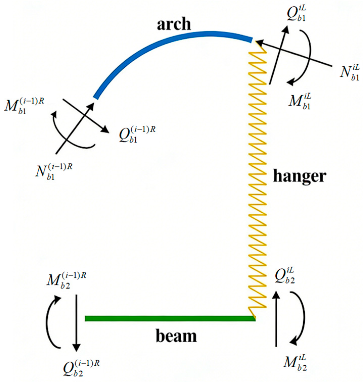
Considering a single beam–arch segment within an arbitrary span, specifically the j-th load-transfer segment located between the i-th and (i + 1)-th hangers, the load-transfer mechanism is illustrated in Figure 2.

In Equation (5), for the left-end section of an arbitrary beam–arch segment—i.e., when the arch segment corresponds to central angle $\theta =0$ and the girder segment to length $x=0$—we have:

$$Z_b^{(i-1)R}=T^{0}C$$

(6)

$$Z_b^{iL}=U^i{Z}_b^{(i-1)R}$$

(7)

where $U^i$ is the segment transmission matrix within the j-th beam–arch segment, representing the displacement–force transmission relation within that segment, and $Z_b^{(i-1)R}$ and $Z_b^{iL}$ are the initial and final positions of the j-th segment, whose state vectors are:

$$Z_b^{(i-1)R}=\left[U_{b1}^{(i-1)R},V_{b1}^{(i-1)R},{\theta }_{b1}^{(i-1)R},M_{b1}^{(i-1)R},Q_{b1}^{(i-1)R},N_{b1}^{(i-1)R},V_{b2}^{(i-1)R},{\theta }_{b2}^{(i-1)R},M_{b2}^{(i-1)R},Q_{b2}^{(i-1)R}\right]$$

(8)

$$Z_b^{iL}=\left[U_{b1}^{iL},V_{b1}^{iL},{\theta }_{b1}^{iL},M_{b1}^{iL},Q_{b1}^{iL},N_{b1}^{iL},V_{b2}^{iL},{\theta }_{b2}^{iL},M_{b2}^{iL},Q_{b2}^{iL}\right]$$

(9)

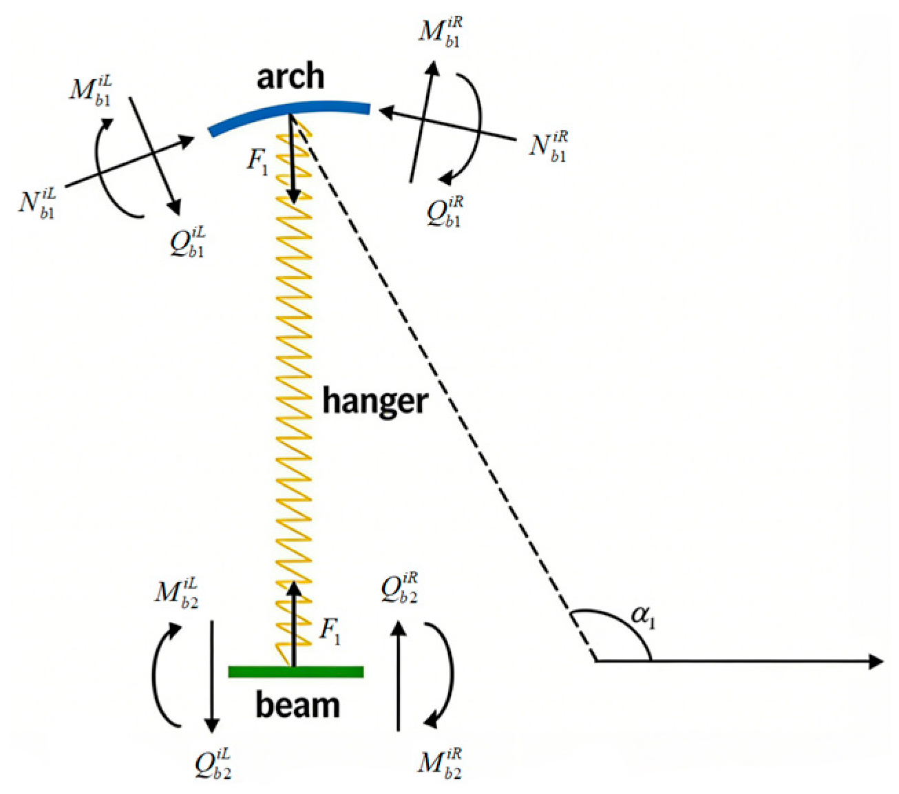
Next, related forces and displacements on both sides of each node will be introduced. Selecting the local node at the i-th hanger for force analysis (as shown in Figure 3), the equilibrium equation at the local node of the i-th hanger can be written as

$$Z_b^{iR}=K^i{Z}_b^{iL}$$

(10)

where $K^i$ is the point transmission matrix at the i-th hanger, expressing the transmission relation of nodal displacement and force and $Z_b^{iR}$ is the state vector at the right end of the beam–arch segment adjacent to the i-th hanger, expressed as

$$Z_b^{iR}=\left[U_{b1}^{iR},V_{b1}^{iR},{\theta }_{b1}^{iR},M_{b1}^{iR},Q_{b1}^{iR},N_{b1}^{iR},V_{b2}^{iR},{\theta }_{b2}^{iR},M_{b2}^{iR},Q_{b2}^{iR}\right]$$

(11)

Based on the field and point matrices, combining Equations (10) and (11) yields:

$$Z_b^{iR}=T^i{Z}_b^{(i-1)R}$$

(12)

where $T^i=K^i{U}^i$ denotes the element transfer matrix of the j-th beam–arch segment corresponding to transmission from the right-end section at the i-th hanger to the right-end section at the (i + 1)-th hanger.

Using the transfer-matrix method, the global bridge model is conceptually divided span by span and reconnected through rigid coupling constraints. Accordingly, the multi-span beam–arch composite system is decomposed into a series of single-span subsystems, with the full transfer matrix of each span derived and subsequently assembled. Ultimately, combining the natural boundary conditions at both ends of the bridge and the inter-segment coupling boundary conditions, the global eigenvalue equation is formulated. The overall transfer matrix of a single-span beam–arch bridge is obtained by sequentially multiplying the element transfer matrices of the serially connected beam–arch segments, expressed as

$$T={\displaystyle \prod _{i=1}{T}^i}$$

(13)

Finally, imposing displacement compatibility and reciprocal contact force equilibrium as interfacial joint constraints, the coupled governing equations are solved iteratively via the Newmark-β method, with convergence monitored and controlled based on interface displacement:

$${\displaystyle \frac{\left|Z_{t+\Delta t}-Z_t\right|}{\left|Z_t\right|}}⩽\xi$$

(14)

where $Z_{t+\Delta t}$ and $Z_t$ are the displacements of the bridge–vehicle contact point at times t and t + Δt, respectively, and $\xi$ is the convergence tolerance, taken as 0.01.

3. Characteristics Indexes

3.1. Dynamic Amplification Factor (DAF)

In addition to calculating the dynamic responses of the vehicle and bridge subsystems, the DAF is commonly introduced to quantify the amplification of structural mechanical effects induced by moving vehicles in vehicle–bridge coupled vibration analysis. DAF serves as a critical theoretical basis for bridge engineering design and operational condition assessment.

Extensive research on DAF has been carried out through field measurements, numerical simulations, and hybrid analytical methods [16]. Field testing can generate the most credible DAF data, yet it entails substantial resource consumption and high costs. In contrast, numerical simulation features significantly lower economic costs, and with the rapid progress of computational technology and the maturity of finite element theory, it has gained growing popularity among researchers and engineering practitioners. Thus, the numerical simulation is used herein to investigate the vehicle–bridge interaction characteristics for the beam–arch composite continuous rigid-frame bridge.

Various definitions of DAF have been proposed in the existing literature [17]. This study adopts a widely accepted DAF definition, as presented in Equation (15), expressed as

$$\mathrm{DAF}=1+\mu ={\displaystyle \frac{Y_{\mathrm{d} \max }}{Y_{j\max }}}$$

(15)

where DAF is the Dynamic Amplification Factor; $Y_{\mathrm{d} \max }$ is the peak dynamic effect and $Y_{j\max }$ is the corresponding peak static effect under the same vehicle(s); and $\mu$ is the impact factor.

3.2. Ride Comfort Index

During vehicle operation, the ride comfort of drivers and passengers fluctuates with vibration intensity. Acceleration measured at key body contact points is conventionally adopted as the evaluation metric for human vibration exposure, and a discomfort indicator—namely the ride comfort index—is accordingly defined. Loprecipe et al. [18] demonstrated that the ISO 2631 [19] methodology is applicable for assessing ride comfort under low-speed conditions. Given that the vehicle speed range considered in this study is 60–90 km/h (relatively low), the ISO 2631 standard is employed herein. This standard evaluates ride comfort via the total weighted root mean square (RMS) acceleration, by establishing body-axis coordinate systems corresponding to 12 vibration transmission directions through components including the seat back, seat pan, and footrest. The RMS accelerations along each axis are weighted and integrated to derive the total weighted RMS acceleration, which quantifies the overall ride comfort level. The corresponding expression is

$$a_v={\left[{(k_1{a}_{\omega 1})}^2+{(k_2{a}_{\omega 2})}^2+{(k_3{a}_{\omega 3})}^2\right]}^{1/2}$$

(16)

where $k_i$ denotes the weighting factors per ISO 2631 for each directional axis; $k_1$, $k_2$ and $k_3$ are the weighting coefficients for vertical, pitch, and lateral accelerations, respectively; and $a_{\omega i}$ signifies the RMS acceleration in the i-th degree of freedom (DOF) across the entire analysis duration. Based on the total weighted RMS acceleration, ride comfort is classified into six levels. The threshold values of human comfort level classifications in a vibration environment are specified in

Table 1. Human comfort level classification in vibration environment [20].

RMS (m/s2)	Human Comfort Level
<0.315	comfortable
0.315–0.63	slightly uncomfortable
0.5–1.0	rather uncomfortable
0.8–1.6	uncomfortable
1.25–2.5	fairly uncomfortable
>2.0	very uncomfortable

.

4. Vehicle–Bridge Coupled Analysis Model

4.1. Bridge and Vehicle Parameters Adopted

The reference bridge has a total length of 860 m, with a span arrangement of 90 m + 170 m × 4 + 90 m. The main superstructure adopts a prestressed concrete variable-depth split single-cell box girder, with an overall deck width of 41.6 m. The single-box single-cell cross-section features a girder depth of 9.5 m at the pier root and 3.8 m at midspan. The bottom slab thickness ranges from 35 cm at midspan to 90 cm at the pier root. The theoretical centroidal axis of the arch rib follows a sinusoidal curve, with a rise of 27 m and a rise-to-span ratio of approximately 1/6.296. Each main span is equipped with 11 pairs of hangers, amounting to 44 pairs across the entire bridge; the standard longitudinal hanger spacing is 8 m, reduced to 7.5 m at midspan, while the transverse spacing is set at 29.5 m.

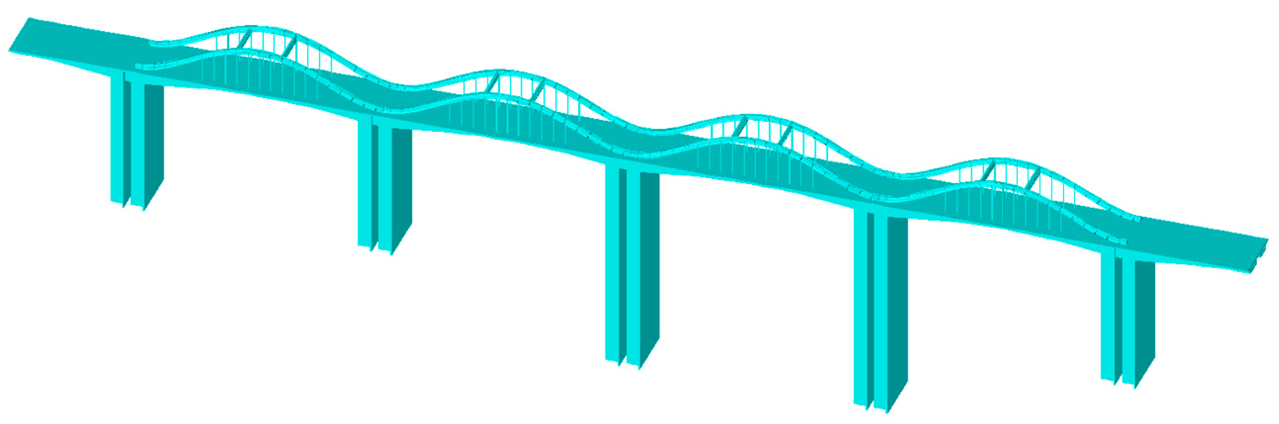
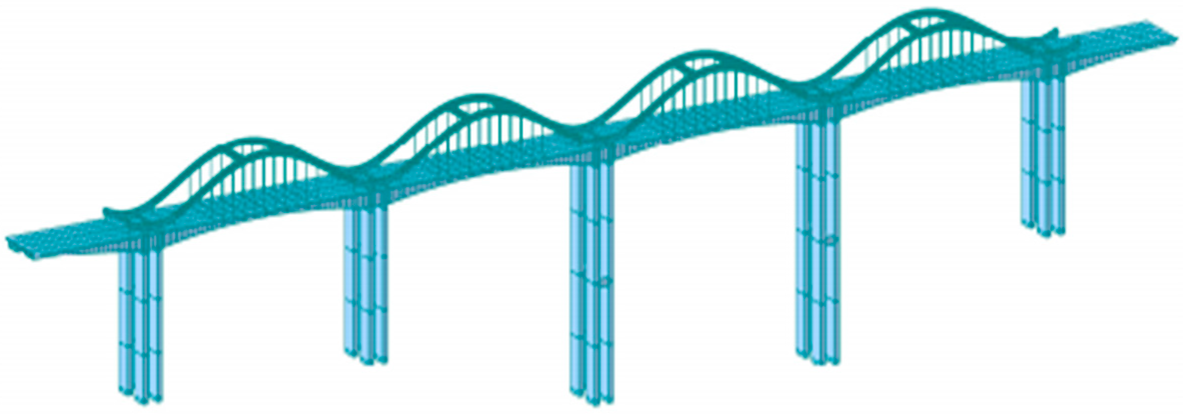
A finite element (FE) model of the bridge was established using ANSYS software, as illustrated in Figure 4. In this numerical model, both the main girder and arch ribs are simulated using BEAM188 elements, hangers are modeled via LINK10 elements, and second-stage dead loads are represented by MASS21 elements. The main girder is constructed of C50 grade concrete, the steel arch ribs are made of Q345q structural steel, and the hangers are fabricated from 1860 MPa steel strands. The material properties for this bridge are summarized in

Table 2. Material properties.

Material	Density (kg/m3)	Elastic Modulus (GPa)	Poisson’s Ratio
C50 Concrete	2450	35	0.2
Q345q Steel	7850	206	0.3
1860 MPa Steel Strand	7850	195	0.3

. Rigid connections are defined between the main girder and piers, while the coupling between hangers and the girder/arch ribs is implemented through node coupling via the CP command. Full fixity is applied at the pier bottoms for considering the boundary conditions. For each hanger, independent parameter arrays and real constants are defined to enable convenient adjustment of initial prestress and subsequent post-processing data extraction. To confirm the optimum length of mesh size for the FEM model, three sizes, 0.5, 1, and 2 m, are employed for the mesh sensitivity analysis. From the results, the differences in the computed results were within 1% across all three cases. To balance computational cost and the need for adequate model resolution, the mesh size of 1m is selected for the remainder studies.

To ensure the accuracy and reliability of the ANSYS bridge model, a MIDAS-based finite element model was established as well. The Midas model was established by the design institute and has undergone rigorous review during the design approval process, providing a reliable benchmark for numerical verification. In the MIDAS model, the main girder and main arch are simulated by using beam elements, while the hangers are modeled as tension-only cable elements. The material properties, section types, and boundary conditions adopted in the MIDAS model were kept consistent with those adopted in the ANSYS model. The established MIDAS finite element model was shown in Figure 5, and the comparison diagram of point positions for the two models was plotted in Figure 6.

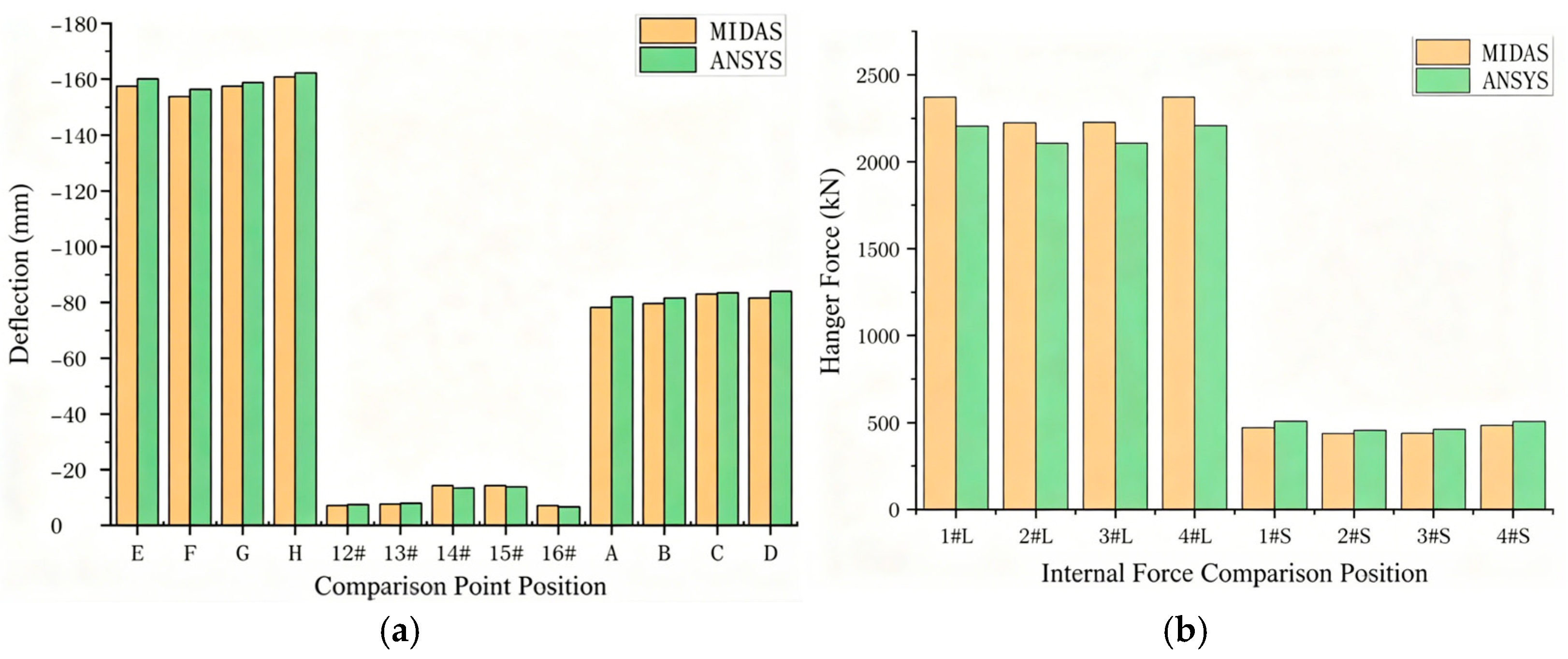
The comparisons results between the MIDAS and ANSYS models for the deflection and hanger forces are presented in Figure 7a and Figure 7b, respectively. With the two models, the maximum difference in the deflection at the arch crown and midspan of the main girder is 3.8%, and the maximum difference in hanger forces is 4.9%. The discrepancies at all control nodes are within 5%. The cross-platform consistency demonstrates that: (1) the geometric modeling, material properties, and boundary conditions in the ANSYS model are correctly implemented; (2) the structural stiffness and mass distribution are accurately represented; and (3) the fundamental static and dynamic characteristics of the bridge are reliably captured. Thus, the verified structural parameters form a solid foundation for the subsequent vehicle–bridge interaction analysis.

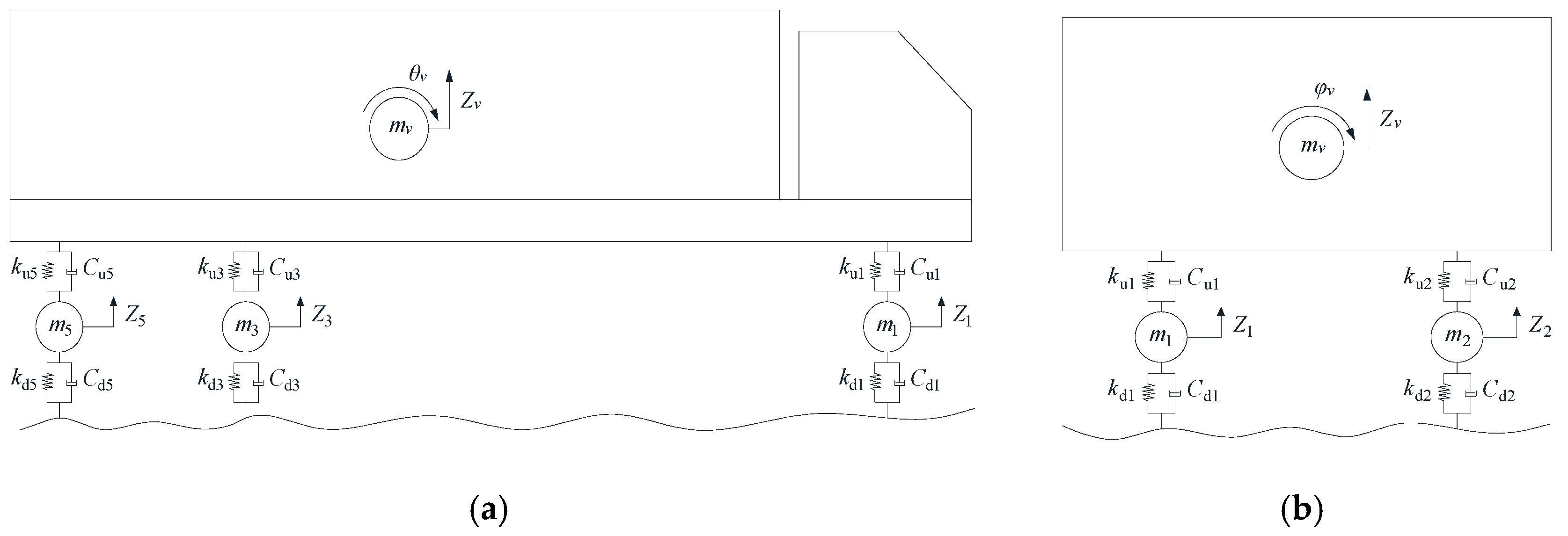
Highway vehicles are classified based on axle number, axle spacing, gross vehicle weight, and other key parameters. When simplified as mass–spring–damper dynamic systems, different vehicle types correspond to distinct parameter sets, including vehicle masses, inter-axle distances, spring stiffness values, and damping coefficients, all of which exert significant impacts on vehicle–bridge coupled vibration responses. In this study, a 3-axle spatial vehicle model is employed for the coupled dynamic analysis [21], with the computational vehicle model schematic depicted in Figure 8.

In the schematic, the symbols are defined as follows: m₁–m₆ represent the wheel masses (incorporating suspension components); ku₁–ku₆ denote the upper spring stiffnesses for each wheel; kd₁–kd₆ refer to the lower spring stiffnesses for each wheel; Cu₁–Cu₆ are the damping coefficients of the upper springs; Cd₁–Cd₆ represent the damping coefficients of the lower springs; Z₁–Z₆ signify the vertical displacements at wheel–bridge contact points; m_v denotes the vehicle body sprung mass; Z_v is the vertical displacement of the vehicle body; θ_v represents the pitch rotation of the vehicle body; and φ_v refers to the roll rotation of the vehicle body. The parameter values for the vehicle model are listed in

Table 3. Parameter values for the vehicle model.

Parameters	Value	Unit	Parameters	Value	Unit
m1–m2	297	kg	Cu1–Cu2	2730	N·s/m
m3–m4	466	kg	Cu3–Cu4	3800	N·s/m
m5–m6	466	kg	Cu5–Cu6	3800	N·s/m
mc	30,542	kg	Cd1–Cd2	2300	N·s/m
Ic1	55,259	kg·m2	Cd3–Cd4	2300	N·s/m
Ic2	6893	kg·m2	Cd5–Cd6	2300	N·s/m
ku1–ku2	630,000	N/m	kd1–kd2	2,800,000	N/m
ku3–ku4	790,000	N/m	kd3–kd4	2,800,000	N/m
ku5–ku6	790,000	N/m	kd5–kd6	2,800,000	N/m
md1–md2	65	kg	md3–md6	75	kg

.

4.2. Bridge Modal Analysis

Prior to the coupled dynamic analysis, modal analysis is performed on the reference bridge to identify its structural stiffness and dynamic characteristics. Owing to the complexity of the bridge structure, high-order mode shapes present diverse coupling modes. Thus, the first ten modes are extracted and analyzed in this study. The natural frequencies and qualitative descriptions of the corresponding mode shapes are summarized in

Table 4. First ten natural frequencies and their mode descriptions.

Mode No.	Frequency (Hz)	Mode Description
1	0.23786	Global longitudinal sway
2	0.30936	In-plane lateral sway of main girder
3	0.41370	Anti-symmetric lateral bending of arches in spans #2 and #4
4	0.43907	Lateral bending of arch in span #1
5	0.44674	Global anti-symmetric lateral bending of arches
6	0.46699	Lateral bending of arch in span #3
7	0.49639	Anti-symmetric lateral bending of arches in spans #2 and #4
8	0.61501	Symmetric lateral bending of arch and girder in span #1
9	0.64493	Lateral bending of main girder
10	0.77034	Vertical bending in span #3

.

To facilitate straightforward comparative analysis under varying parametric conditions, this study adopts the code-specified impact factor to define the reference DAF. In accordance with the General Specifications for Design of Highway Bridges and Culverts (JTG D60-2015), the impact factor is correlated with the bridge’s natural vibration properties, and the codified formula is presented in Equation (17):

$$\mu =\left\{\begin{array}{ll}0.05,& f\le 1.5\mathrm{Hz}\\ 0.1767\ln f-0.0157,& 1.5\mathrm{Hz}\le f\le 14\mathrm{Hz}\\ 0.45,& f\ge 14\mathrm{Hz}\end{array}\right.,$$

(17)

Combining Table 4 with Equation (17), all the first ten natural frequencies are below 1.5 Hz. Accordingly, the code-specified impact factor is taken as φ = 0.05. Substituting yields a reference DAF of 1.05, which is adopted as the benchmark for comparative analyses in subsequent sections.

4.3. Comfirming Evaluation Sections

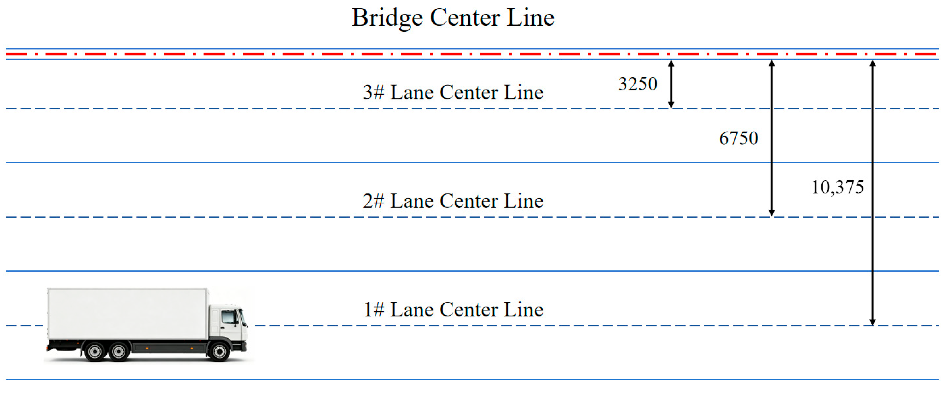
Within a vehicle–bridge coupled vibration system, the vehicle serves as the primary excitation source, while the bridge acts as the load-bearing structure. Fluctuations in both vehicle and bridge parameters can substantially alter the coupled dynamic responses. Existing research demonstrates that the impact factor reaches its maximum under single-vehicle loading conditions [22]. Accordingly, this chapter takes a single 3-axle truck as the research object, investigating the effects of diverse vehicle and bridge parameters on the DAF of girder–arch composite bridge components. The lane loading layout is illustrated in Figure 9.

During vehicle passage, vibrations occur in the main girder, arch ribs, hangers and piers of the beam–arch composite bridge, which directly govern the coupled dynamic responses. The main girder and arch ribs serve as primary load-bearing members, featuring intricate stress states and significant vibration responses. Hangers act as critical force-transmission components between the girder and arch, with complex axial force conditions and represent key safety control members. For the studied bridge, the tall main piers possess relatively low longitudinal stiffness and exhibit remarkable longitudinal displacements, necessitating targeted investigation.

Therefore, the parametric vehicle–bridge coupling analysis focuses on the following critical sections and key mechanical indicators: vertical displacements at the midspan of each girder segment and arch crown sections, longitudinal displacements at the tops of main piers, and axial tensile forces of midspan hangers in main spans. The locations of these control sections are depicted in Figure 10, with the corresponding section labels and calculated mechanical indicators tabulated in

Table 5. Evaluation sections.

Member	Section	Label	Quantity
Main girder	Midspan of span #2	G2-2	Vertical displacement
	Midspan of span #3	G3-3
	Midspan of span #4	G4-4
	Midspan of span #5	G5-5
Pier top	Pier #12 top	P1-1	Longitudinal displacement
	Pier #13 top	P2-2
	Pier #14 top	P3-3
	Pier #15 top	P4-4
	Pier #16 top	P5-5
Main arch	Arch crown of span #2	A1-1	Vertical displacement
	Arch crown of span #3	A2-2
	Arch crown of span #4	A3-3
	Arch crown of span #5	A4-4
Hanger	Midspan hanger of span #2	Red	Axial tensile force
	Midspan hanger of span #3	Yellow
	Midspan hanger of span #4	Green
	Midspan hanger of span #5	Blue

.

Given that the bridge is located on an expressway with a minimum speed limit of 60 km/h and heavy trucks typically operate at moderate speeds, 80 km/h is selected as the representative vehicle speed for analysis. Existing studies indicate that vertical displacements and impact factors rise significantly with increasing deck roughness severity [23]. Moreover, the likelihood of vehicle jumping surges sharply when deck roughness is inferior to Class B [24]. As vehicle jumping is prohibited on expressways, Class B deck roughness is adopted in this analysis. The truck weight is set to 33 t in accordance with Section 2.2, and the baseline analytical conditions are summarized in

Table 6. Typical condition.

Vehicle Type	Speed	Gross Mass	Deck Class	Lane
Three-axle truck	80 km/h	33.0 t	Class B	1#

.

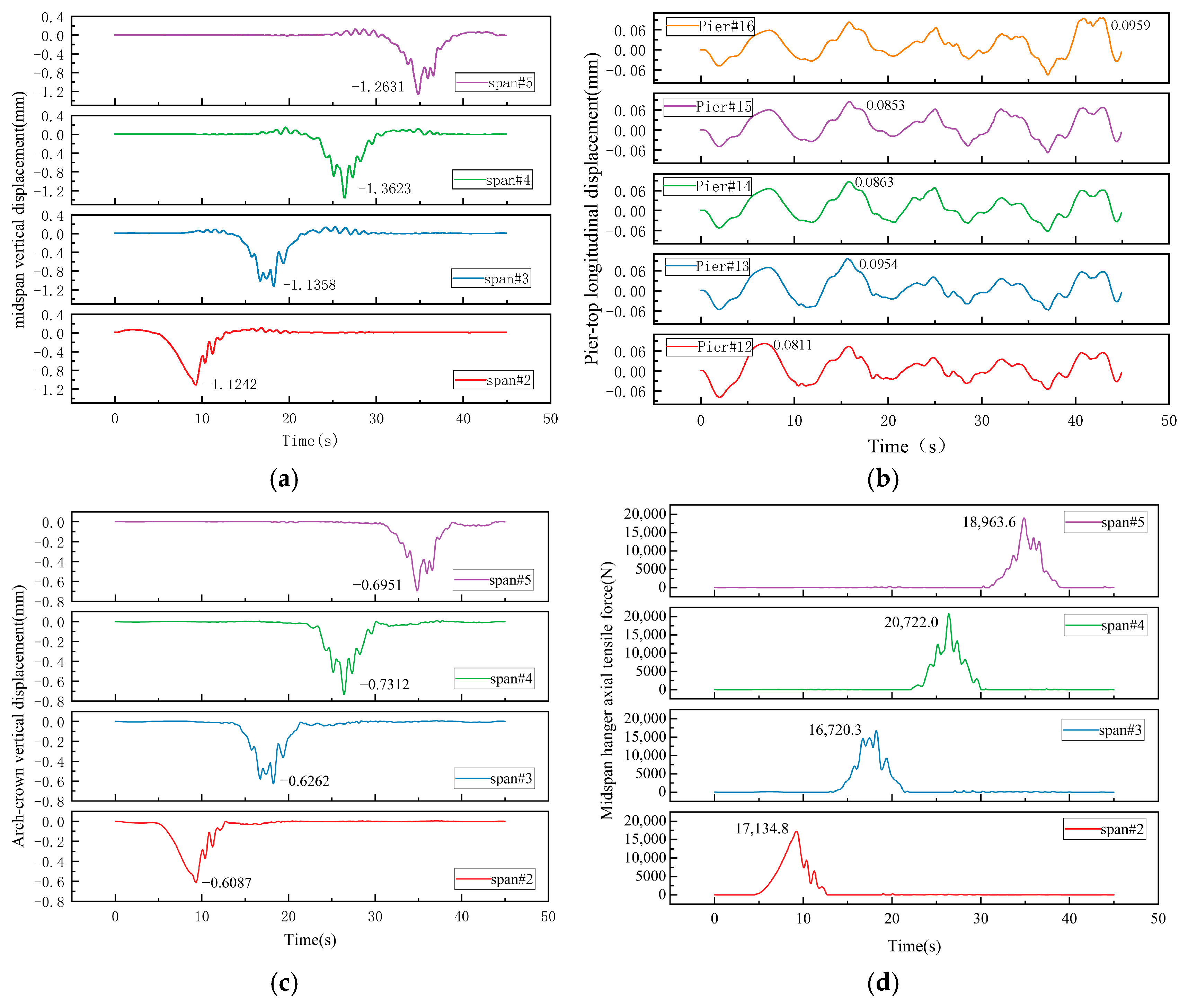
Under this typical working condition, the coupled dynamic solver is adopted to calculate the dynamic responses at all control sections, and the time histories of the corresponding responses are presented in Figure 11. In these figures, the vertical axis represents the target response variable, while the horizontal axis denotes time corresponding to the constant-speed movement of the vehicle.

Figure 11 reveals that the response time histories share similar qualitative variation trends, yet differ in peak occurrence times and amplitude magnitudes. Accordingly, for each category of dynamic response, the section with the maximum absolute peak value is selected as the critical control section. Specifically, Span #4 presents distinctly larger peak values for midspan vertical displacement, arch-crown vertical displacement and midspan hanger axial force compared with other spans, while Pier #16 registers the largest peak value for pier-top longitudinal displacement.

Consequently, the critical control sections for each key response indicator are determined as follows: the midspan of Span #4 for main girder midspan vertical displacement; the arch crown of Span #4 for arch-crown vertical displacement; the midspan hanger of Span #4 for midspan hanger axial force; and the top of Pier #16 for pier-top longitudinal displacement.

For brevity, only the peak dynamic responses and corresponding DAFs at the above-defined control sections are extracted for statistical analysis and comparative assessment. Herein, peak values are defined as the maximum absolute magnitudes extracted from each response time-history curve.

5. VBI Characteristics Under Various Parameters

5.1. Effect of Vehicle Speed

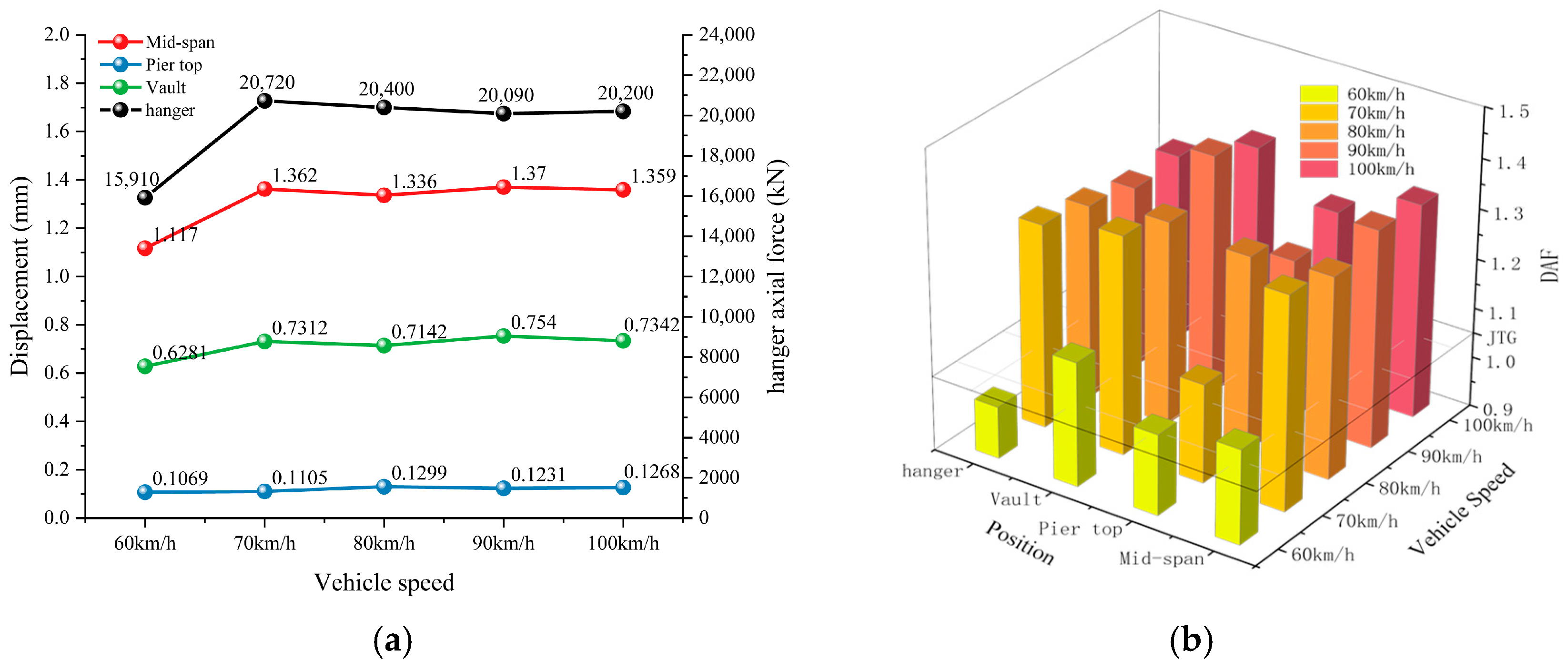
As a moving vehicle traverses the bridge, varying travel speeds induce distinct degrees of dynamic impact. For expressways, the operating speed of trucks is typically no less than 60 km/h, and 3-axle heavy trucks generally run at moderate velocities owing to their large gross mass. To investigate the effects of vehicle speed on the coupled dynamic responses and DAFs, five constant speeds—60, 70, 80, 90, and 100 km/h—are selected for parametric analysis. The analysis adopts a fixed gross truck mass of 33.0 t and Class B deck roughness, with the 3-axle truck traveling steadily in Lane #1 at the aforementioned speeds. The corresponding peak dynamic responses, DAF values, and ride comfort indices are plotted in Figure 12 and tabulated in

Table 7. Ride comfort indexes for various vehicle speeds.

Vehicle Speed	60 km/h	70 km/h	80 km/h	90 km/h	100 km/h
Ride comfort index	0.79	1.14	1.16	1.33	1.42

.

From Figure 12, the midspan vertical dynamic responses under variable vehicle speeds can be divided into two distinct phases. The first phase corresponds to a speed of 60 km/h, where both the peak dynamic response and DAF reach their minimum values. The phenomenon can be attributed to the interaction between vehicle excitation frequency and structural dynamic characteristics. At 60 km/h, the excitation frequency generated by the vehicle axle passages coincides with an anti-resonance condition of the vehicle suspension system, which minimizes the dynamic wheel load transmitted to the bridge deck. The second phase covers the speed range of 70–100 km/h. Within this interval, the dynamic responses vary by merely 2% but are approximately 22% greater than those in the first phase. This relatively stable response plateau occurs because the bridge’s fundamental vertical frequency (0.77 Hz) is substantially lower than the dominant excitation frequencies at these speeds, placing the system in a sub-resonant regime where the structural response is insensitive to further speed increases. Similar two-phase response patterns have been reported by Wang et al. [25] and Li et al. [26] for bridges with comparable dynamic characteristics. Analogous variation trends are also observed in arch crown vertical displacement and hanger axial force. For pier-top longitudinal displacement, both the peak dynamic response and DAF first increase sharply between 70 and 80 km/h, and then decline from 80 to 90 km/h. Below about 70 km/h, the longitudinal forces are too weak to excite the bridge’s longitudinal vibration modes. Above this threshold, the excitation intensity and frequency effectively trigger the longitudinal dynamic response, causing an abrupt rise. This fluctuation is especially prominent in the DAF, implying that the static component of this response is negligible, thus amplifying the dynamic characteristics reflected in the DAF.

As presented in Table 7, the ride comfort index attains its minimum at 60 km/h, signifying the optimal riding comfort. With escalating speed, the ride comfort deteriorates gradually, and the index peaks at 100 km/h, corresponding to the worst comfort condition.

In summary, the variation trends of peak dynamic responses and DAFs are highly consistent across different vehicle speeds, both exhibiting an overall upward tendency with increasing speed. The 60 km/h scenario constitutes the safest operating condition. Nevertheless, a sharp surge in structural dynamic responses and corresponding DAFs occurs when the speed rises from 60 to 70 km/h. Beyond 70 km/h, the DAFs for all monitored indicators stabilize with negligible further fluctuations. Additionally, the vehicle acceleration RMS value increases monotonically with speed, verifying that elevated speeds impair ride comfort. Accordingly, a conservative amplification of the dynamic impact factor is recommended for heavy vehicle crossing assessments, especially for speeds exceeding 60 km/h.

5.2. Effect of Vehicle Weight

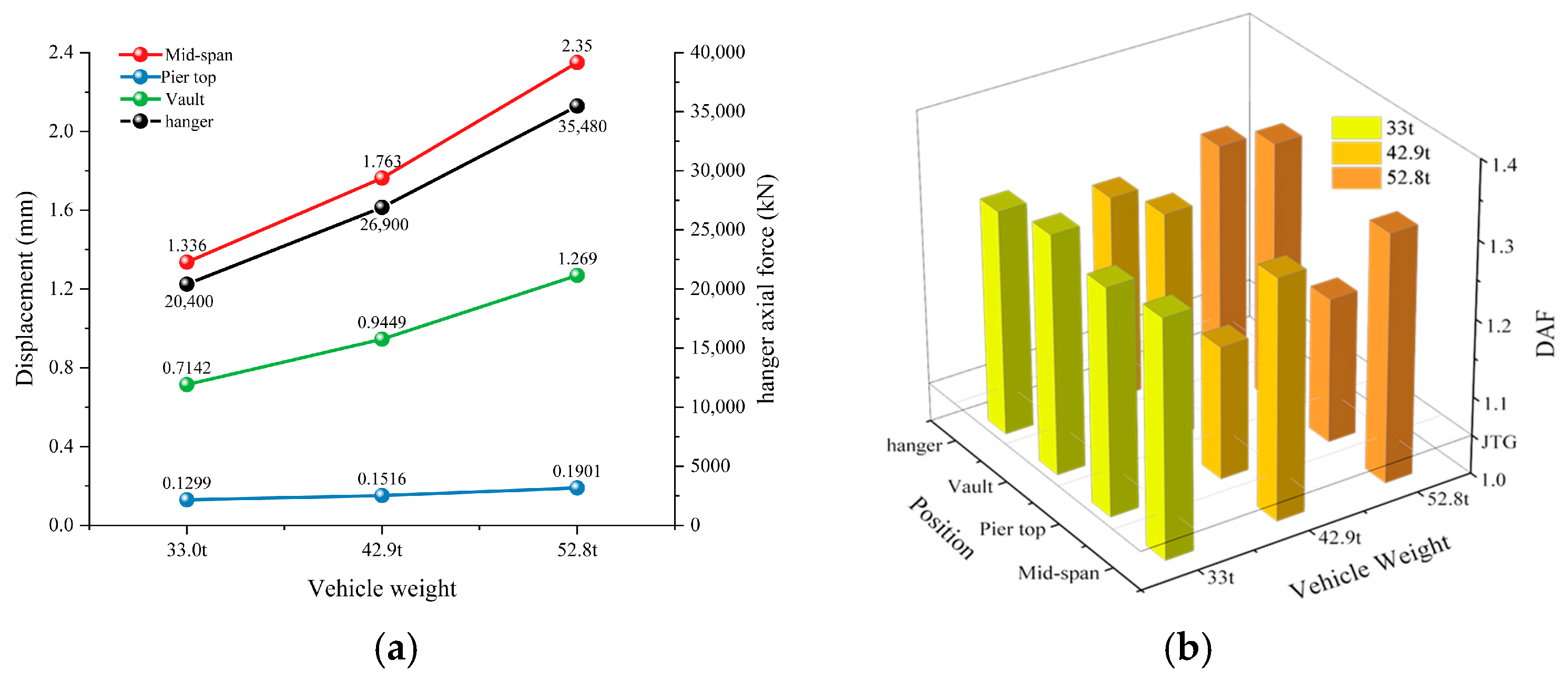
With the expansion of highway freight transportation, trucks are characterized by increasingly higher operating speeds and heavier loading capacities, imposing stricter performance requirements on bridge design. Heavier vehicles generate greater static load effects, and their high-speed movement can further induce amplified dynamic responses in bridge structures. To quantify the effects of overweight trucks on structural dynamic responses and DAFs, three gross vehicle weights are selected for parametric analysis: the baseline weight of 33.0 t, a 30% increase (42.9 t), and a 60% increase (52.8 t). The running speed of the vehicle is set to 80 km/h. All other analytical parameters remain consistent with those specified in Section 5.1. Based on these parameters, the peak dynamic responses and DAF values are presented in Figure 13, with the ride comfort indices tabulated in

Table 8. Ride comfort indexes for various vehicle weights.

Vehicle Weight	33 t	42.9 t	52.8 t
Ride comfort index	1.16	1.28	1.31

.

As depicted in Figure 13a, the influence of vehicle weight on the DAF differs distinctly from its effect on structural dynamic responses. As the vehicle weight increases from the baseline value to 1.6 times the base weight, the peak dynamic responses of all monitored indicators rise substantially: midspan vertical displacement increases by 75.90%, pier-top longitudinal displacement by 46.34%, arch-crown vertical displacement by 77.68%, and hanger axial force by 73.92%. These results verify that vehicle weight exerts a remarkable impact on the bridge’s dynamic responses.

From Figure 13b, the variation patterns of DAF for all structural effects diverge sharply from those of peak dynamic responses. At the pier-top section, a pronounced negative correlation between DAF and vehicle weight is observed, where the DAF exhibits a reduction of approximately 9% with vehicle weight increasing. This behavior can be explained by the inertial damping effect, implying that heavier vehicles possess greater inertia to resist high-frequency vibrations, and the dynamic component of the bridge response can be effectively suppressed. Thus, while both static and dynamic responses increase with vehicle weight, the static component grows at a faster rate, leading to a decreased DAF ratio. A similar phenomenon has also been observed in the studies by Deng [22] and Kalin et al. [27].

Table 8 shows that when the vehicle weight increases from 33 t to 52.8 t (a 60% rise), the ride comfort index only elevates by 12.9%, implying a slight degradation in ride comfort with the growth of vehicle weight.

In summary, the increase in vehicle weight imposes a minimal impact on ride comfort, yet it significantly amplifies the bridge’s dynamic responses without exerting an obvious effect on the DAF. This phenomenon occurs because heavier vehicles induce larger static and dynamic responses; under identical vehicle speed conditions, the movement of heavier vehicles may restrain the bridge’s dynamic responses via mechanisms such as inertial damping. Accordingly, as vehicle weight increases, the growth rate of dynamic responses is lower than that of static responses in DAF calculation. Nevertheless, the rise in vehicle weight leads to enhanced bridge dynamic responses, which may threaten structural safety even with slight variations in the DAF.

5.3. Effect of Lane Eccentricity

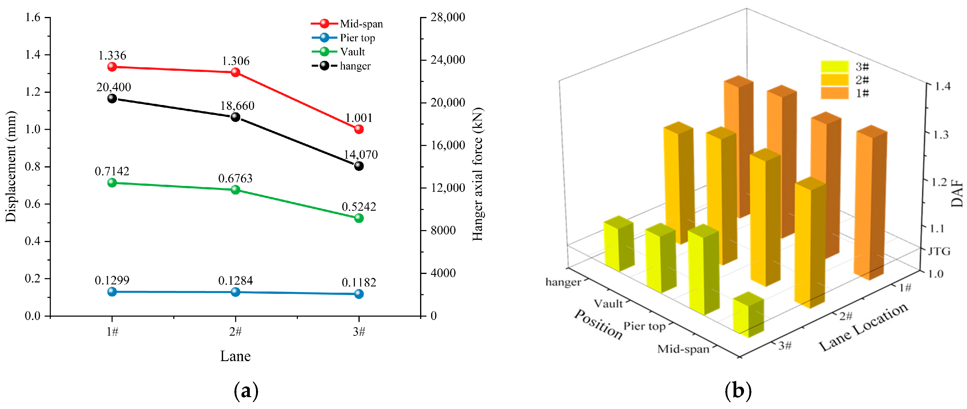
Based on the bridge drawings and design parameters, three loading lanes are defined in this analysis. The distances from the centerline of each lane to the cross-sectional centroid of the main girder are as follows: 10.375 m for Lane #1, 6.75 m for Lane #2, and 3.25 m for Lane #3. The vehicle travel speed is set to 80 km/h with a gross mass of 33.0 t, and all other analytical parameters remain consistent with those specified in Section 5.1. The corresponding peak dynamic responses and DAFs for various lane eccentricities are presented in Figure 14, respectively, with the ride comfort indices tabulated in

Table 9. Ride comfort indexes for various lane eccentricities.

Lane Location	1#	2#	3#
Ride Comfort Index	1.16	1.18	1.19

.

As depicted in Figure 14a, the peak dynamic responses of all monitored indicators decrease gradually as the vehicle traverses laterally from Lane #1 to Lane #3. Notably, the magnitude of response reduction from Lane #2 to Lane #3 is far more pronounced than that from Lane #1 to Lane #2. Specifically, the peak midspan vertical displacement drops by 25.07%, pier-top longitudinal displacement decreases by 9%, and peak arch-crown vertical displacement and hanger axial force decline by 26.60% and 31.03%, respectively.

Figure 14b illustrates that the variation trend of the Dynamic Amplification Factor (DAF) with lateral loading position aligns closely with that of peak dynamic responses. When the vehicle shifts from Lane #1 to Lane #2, the DAF values for all indicators decrease slightly, with the impact factor reducing from six times the code-specified value to five times. A further lateral movement to Lane #3 triggers a more substantial DAF decline, lowering the impact factor to approximately two to three times the codified threshold. These findings demonstrate that the lane eccentricity exerts differential impacts on diverse structural responses. Specifically, vertical responses are highly sensitive, with reductions exceeding 20%, while longitudinal responses only undergo minor fluctuations (less than 10%). The differential sensitivity arises from the distinct load transfer mechanisms. For the box girder cross-section, the vertical responses are directly coupled with the torsional behavior. For this, the vertical responses are amplified under the eccentric loads. In contrast, longitudinal pier-top displacements are governed by the overall longitudinal stiffness of the rigid-frame system, which is largely independent of transverse load position.

As presented in Table 9, the ride comfort index varies by less than 2.6% across all three lanes, indicating that the vehicle’s lateral lane position has no significant effect on riding comfort.

In summary, the correlations between lateral offset and both peak dynamic responses and DAF values are nonlinear: as the vehicle moves toward the bridge centerline (i.e., eccentricity diminishes), the decay rate of dynamic responses accelerates. Conversely, transverse vehicle positioning exerts negligible influence on ride comfort. Vehicles traveling in the outermost lane, with the largest offset from the bridge centerline, induce the most severe vertical structural responses. Since elevated DAF values correspond to a reduced structural safety margin and heightened risks of excessive vibration or cracking, strict management of vehicle travel trajectories is required in bridge operation. In particular, the simultaneous passage of multiple heavy vehicles in the edge lanes should be prohibited to safeguard structural safety during service.

5.4. Effect of Pavement Roughness Level

The pavement roughness is modeled as a zero-mean, stationary Gaussian random process. Using the inverse Fourier transform method, the continuous roughness profile $r_i(x)$ can be simulated as in Equation (18):

$$\left|r_i(x)\right|=\sqrt{{\displaystyle \frac{N}{2\Delta l}}{G}_x(n_i)}\hspace{1em}(i=0,1,2,\dots ,{\displaystyle \frac{N}{2}}),$$

(18)

where $\left|r_i(x)\right|$ is the amplitude of the i-th frequency component; $N$ is the number of sampled frequency bands; $G_x(n_i)$ is the discrete form of the power spectral density function, with $n_i=i\Delta n$, $\Delta n={\displaystyle \frac{1}{L}}$; $\Delta l$ is the spatial sampling interval, set as $\Delta l\le 0.025$ m (25 mm) to satisfy the sampling theorem; $\Delta n$ is the spatial frequency resolution; and $L$ is the bridge (or simulated deck) length.

After removing any absolute-value sign tied to complex amplitude handling and invoking the discrete Fourier transform, the discrete roughness sequence $r(x)$ is generated via the inverse discrete Fourier transform, as in Equations (19) and (20):

$$r(x)={\displaystyle \frac{1}{N}}{\displaystyle \sum _{i=0}^{N-1}{X}_i{e}^{\frac{2\pi ikm}{N}}} (m=0,1,2,\dots ,N-1),$$

(19)

$$X_i=\left|X_i\right|e^{k{\phi }_i} (i=0,1,2,\dots ,{\displaystyle \frac{N}{2}}),$$

(20)

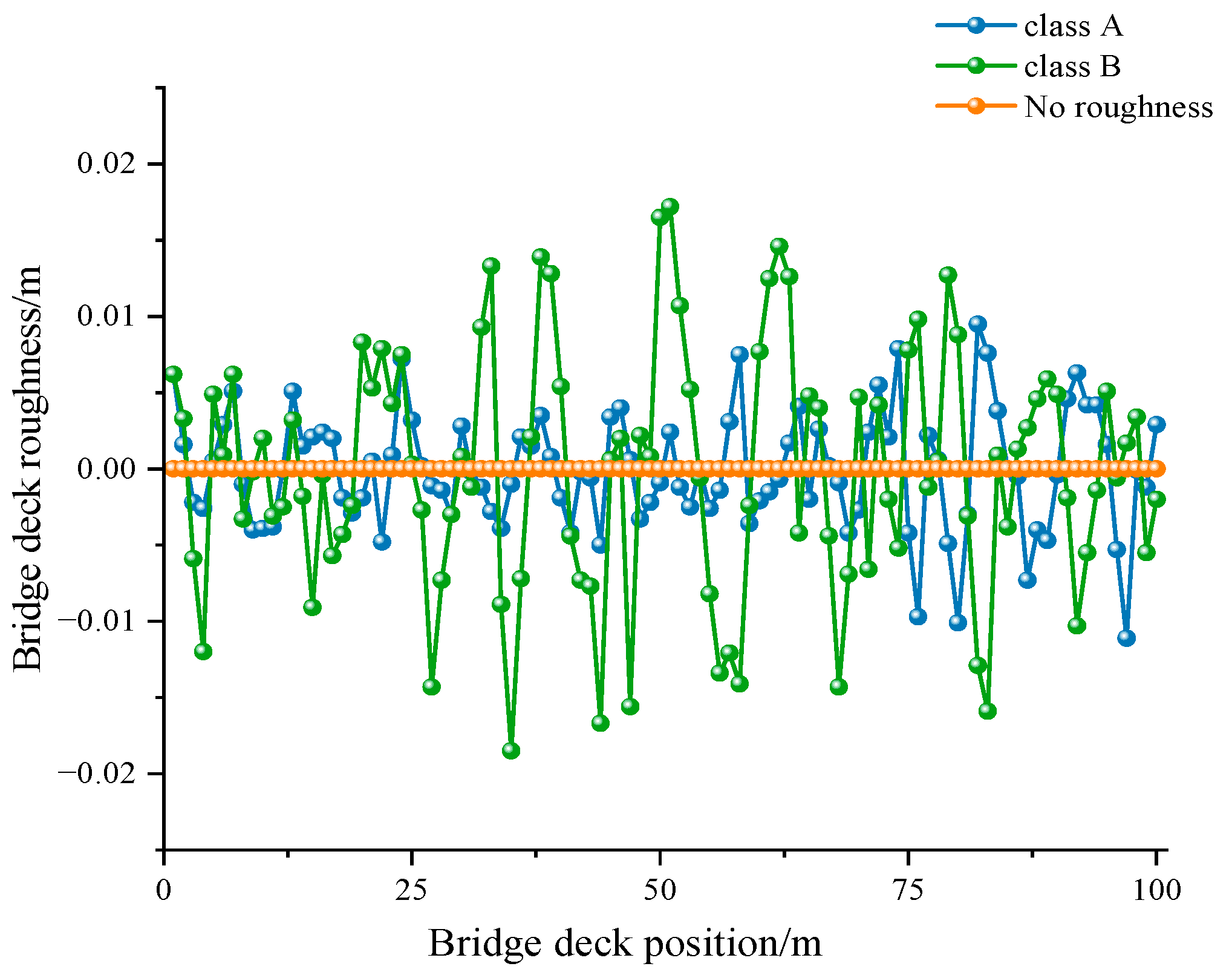
where $r(x)$ is the discrete roughness sequence; ${\phi }_i$ is a random sequence with ${\phi }_i$ independently drawn within $\left[\begin{array}{cc}0& 2\pi \end{array}\right]$. Based on the vehicle’s primary vibration frequency range (0.5–50 Hz) and typical speed range (2.5–50 m/s), the effective spatial frequency range can be determined, yielding the lower and upper bounds $n_d=0.01$ m⁻¹ and $n_u=20$ m⁻¹. The reference spatial frequency $n_0=0.1$ m⁻¹ and the roughness coefficients for different roughness levels were listed in

Table 10. Roughness coefficients for different roughness levels (10⁻⁶ m³).

Pave Roughness Level	No Roughness	Class A	Class B
$G_x(n)$	0	16	64

. The pavement roughness samples for grades A, B, and the case without roughness are shown in Figure 15.

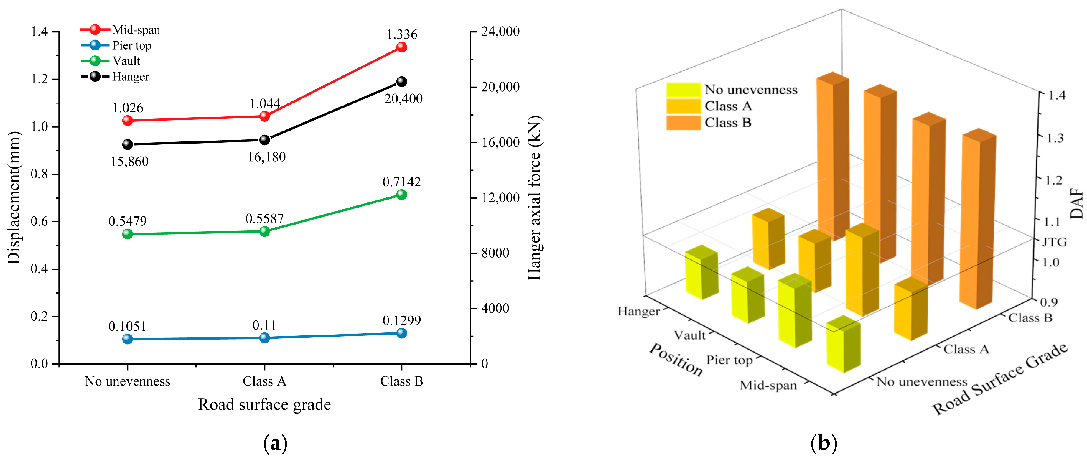
As the primary excitation source in the vehicle–bridge coupled system, vehicle vibration is strongly governed by pavement roughness. With prolonged bridge service, deck surface conditions tend to deteriorate; increased roughness amplifies vehicle vibration, which further intensifies bridge vibration and potentially compromises structural safety. For expressways, the minimum permissible roughness grade is Class B. Accordingly, this section investigates three scenarios: smooth deck (no roughness), Class A roughness, and Class B roughness. A lane eccentricity of 10.375 m (Lane #1) is adopted, with all other analytical parameters consistent with the foregoing settings. The corresponding peak dynamic responses and DAFs under varying pavement roughness levels are presented in Figure 16a and Figure 16b, respectively, and the associated ride comfort indices are tabulated in

Table 11. Ride comfort indexes for various pavement roughness levels.

Pave Roughness Level	No Roughness	Class A	Class B
Ride comfort index	0.56	0.85	1.16

.

As illustrated in Figure 16a, the peak dynamic responses of all monitored indicators exhibit a monotonically increasing trend as the deck surface condition deteriorates from the ideal smooth state to Grade A and further to Grade B. The results are mainly attributed to the fact that a pavement roughness of class A generates disturbances primarily in the low-frequency range, which are effectively filtered by the vehicle suspension system before being transmitted to the bridge. For class B, however, the road samples contain higher energy in the mid-frequency range (typically 1–10 Hz), which overlaps with the primary vibration frequencies of the vehicle body. The mid-frequency excitations pass through the suspension with minimal attenuation and are directly transmitted to the bridge deck as amplified dynamic wheel loads. This frequency-dependent filtering mechanism explains why the transition from class A to class B produces different effects.

As depicted in Figure 16b, the variation trends of DAFs for all indicators align consistently with the deterioration of deck roughness. Under ideal smooth conditions, the DAFs for all vertical response indicators equal 1, indicating no vertical dynamic amplification during vehicle traversal. When the roughness degrades to Grade A, DAFs increase marginally, with pier-top longitudinal displacement registering the maximum increment of approximately 3.8%; although most DAF values remain within the permissible range, the pier-top longitudinal displacement DAF slightly exceeds the code-specified limit. Further deterioration to Grade B roughness leads to a dramatic rise in DAFs, especially for midspan vertical displacement and arch-crown vertical displacement, with increments reaching up to 28.43%.

Table 11 reveals remarkable fluctuations in the ride comfort index across varying deck conditions. Under Grade B roughness, the ride comfort index peaks at 2.07 times that under ideal conditions, highlighting the severe detrimental effect of poor deck surface quality on riding comfort.

In conclusion, the sensitivity of structural dynamic responses to deck roughness intensifies with the degradation of surface conditions. Structural responses are nearly insensitive to Grade A roughness variations, but their sensitivity surges sharply under Grade B conditions, where minor surface deterioration can trigger substantial growth in peak dynamic responses and DAFs. Therefore, strengthening bridge deck maintenance and management is crucial to mitigate the dynamic impacts of moving vehicles, thus preserving the structural integrity and operational safety of bridges

6. Discussion

To further assess the reliability of the computed dynamic responses, the DAF values obtained herein are compared with provisions from different bridge design codes (

Table 12. Values of DAF specified in each code.

Code	Method	DAF
JTG D60-2015 (China) [28]	μ = 0.05 (f < 1.5 Hz)	1.05
AASHTO LRFD (USA) [29]	IM = 33%	1.33
BS 5400 (UK) [30]	IF = 0.25	1.25
Eurocode 1 (Europe) [31]	Included in load model	/
SIA 261 (Switzerland) [32]	Included in load model	/
Present	VBI analysis	1.03–1.34

) and with published studies on analogous bridge types (

Table 13. Comparison of DAF values with published studies on analogous bridge types.

Reference	Bridge Type	Main Span (m)	Fundamental Frequency (Hz)	DAF Range
Zhou et al. [33]	Continuous rigid-frame	206	0.78	1.03–1.09
Gou et al. [34]	Continuous rigid-frame	108	1.56	1.05–1.2
Han et al. [35]	Rigid-frame arch bridge	40	6.02	1.0–1.2
Qin et al. [36]	Concrete arch bridge	180	0.59	1.10–1.4
Present	Deck-arch composite	170	0.77	1.03–1.08

), using the structural parameters of the investigated bridge (fundamental frequency 0.77 Hz, main span 170 m).

As can be seen, the Chinese code JTG D60-2015 specifies an impact factor of 0.05 for bridges with fundamental frequency below 1.5 Hz, corresponding to DAF = 1.05. US AASHTO LRFD gives 1.33, and UK BS 5400 gives 1.25. European EN 1991-2 and Swiss SIA 261 cannot provide explicit DAF values because dynamic effects are embedded in the load models. For the present study, the computed DAF range (1.03–1.34) agrees well with the explicit code values. In addition, the DAF values presented fall within the overlapping range reported for both continuous rigid-frame bridges and arch bridges with similar dynamic characteristics. Therefore, the consistency between numerical results and code-specified values provides additional confidence in validating the vehicle–bridge interaction analysis conducted in this study.

7. Conclusions

This study quantitatively investigates the vehicle–bridge interaction (VBI) characteristics of a six-span beam–arch composite continuous rigid-frame bridge via the ANSYS spatial beam-element model and a three-axle spatial vehicle model, focusing on the effects of vehicle speed, gross weight, loading lane eccentricity, and pavement roughness on structural dynamic responses, dynamic amplification factor (DAF), and ride comfort. Key control sections are identified as the midspan, arch crown and midspan hanger of Span 4, and the top of Pier 16, where the peak dynamic responses of the bridge system concentrate. The main conclusions of the research are as follows:

(1)

Vehicle speed exerts a two-stage nonlinear effect on the bridge’s dynamic responses and DAF. The dynamic responses and DAF reach their minimum at 60 km/h, while a significant 22% increase in dynamic responses is observed in the 70–90 km/h range, with DAF values stabilizing at a high level beyond 70 km/h. Ride comfort degrades monotonically with increasing speed, with the ride comfort index rising continuously as speed increases from 60 km/h to 100 km/h.

(2)

Vehicle gross weight significantly amplifies the peak dynamic responses of the bridge structure but has a negligible impact on DAF and a mild effect on ride comfort. A 60% increase in vehicle weight (from 33.0 t to 52.8 t) leads to a maximum 77.68% rise in structural peak dynamic responses, while the DAF of key control sections varies by no more than 9%, and the ride comfort index only increases by 12.9%. The growth rate of dynamic responses is lower than that of static responses, resulting in the stability of DAF with increasing vehicle weight.

(3)

Transverse loading eccentricity induced by different loading lanes causes asymmetric structural dynamic responses, with a more pronounced impact on vertical responses than longitudinal ones. As the vehicle moves from the outermost Lane 1 to the innermost Lane 3 (toward the bridge centerline), the vertical dynamic responses of the main girder, arch rib and hanger decrease by more than 20%, while the longitudinal displacement of the pier top only decreases by 9%. DAF shows a consistent nonlinear decay trend with dynamic responses, and the lane position has an insignificant effect on ride comfort (variation < 2.6%).

(4)

Pavement roughness is the most critical factor affecting both structural dynamic performance and ride comfort, with the impact intensifying sharply with the deterioration of pavement conditions. Compared with the ideal smooth pavement, Class B roughness leads to a maximum 27.97% increase in peak dynamic responses and a 28% rise in DAF of key sections. The ride comfort index under Class B roughness is 2.07 times that of the smooth state, with the root mean square (RMS) value of ride comfort varying by up to 107%, while Class A roughness only causes a slight increase in structural dynamic responses.

In summary, the beam–arch composite continuous rigid-frame bridge exhibits distinct VBI characteristics under the influence of key vehicle and pavement parameters, with pavement roughness, vehicle speed and loading lane eccentricity being the primary factors governing structural dynamic safety, and pavement roughness dominating ride comfort. The research findings provide a theoretical basis and technical reference for the dynamic design, operational management and maintenance of beam–arch composite continuous rigid-frame bridges. However, this study is primarily a theoretical and numerical investigation; since the experimental condition is limited, field validation will be the focus of our future work.

References

1. Gao, Q.F.; Zhang, K.; Wang, T.; Peng, W.K.; Liu, C.Q. Numerical investigation of the dynamic responses of steel-concrete girder bridges subjected to moving vehicular loads. Meas. Control 2021, 54, 465–484. [Google Scholar] [CrossRef] [Scilit]
2. Sun, L.; Zhao, X.Z. Coupled dynamics of vehicle-bridge interaction system using high efficiency method. Adv. Civ. Eng. 2021, 2021, 1964200. [Google Scholar] [CrossRef] [Scilit]
3. Hou, J.L.; Wang, J.; Xu, W.B.; Chen, Y.J.; Wang, B.; Liu, J.Y.; Shen, B.T.; Li, Y.; Sun, H. An analysis method of vehicle–bridge coupling vibration considering effects of expansion joint parameters and its application. Struct. Control Health Monit. 2022, 29, e3065. [Google Scholar] [CrossRef] [Scilit]
4. Liu, L.; Yang, X.T.; Yan, B.Q.; Miao, S.Y. Dynamic responses of RC girder bridge under heavy truck and seismic loads combined. Sustainability 2022, 14, 9263. [Google Scholar] [CrossRef] [Scilit]
5. Wang, B.T.; Jia, Y.D.; Zhao, H.J.; Wang, S.M.; Jin, Z.C.; Yang, J.F. Research on the dynamic response of a continuous steel box girder bridge based on the ANSYS platform. Sustainability 2022, 14, 10638. [Google Scholar] [CrossRef] [Scilit]
6. González, A.; Covián, E.; Casero, M. Verifying the suitability of uncoupled numerical methods for solving vehicle-bridge interaction problems. Struct. Infrastruct. Eng. 2022, 19, 1407–1424. [Google Scholar] [CrossRef] [Scilit]
7. Erduran, E.; Nordli, C.; Gonen, S. Effect of elastomeric bearing stiffness on the dynamic response of railway bridges considering vehicle-bridge interaction. Appl. Sci. 2022, 12, 11952. [Google Scholar] [CrossRef] [Scilit]
8. Wan, P.; Lei, X.Y.; Wu, W.B.; Hu, Q.Q.; Wan, L.; Li, G.L. Simulation analysis of coupled structural vibration of highway railway combined bridge induced by overlapping action of vehicle and train. Geofluids 2022, 2022, 1986593. [Google Scholar] [CrossRef] [Scilit]
9. Wu, T.Y.; Qiu, W.L.; Wu, H.; Yao, G.W.; Guo, Z.W. Coupled vibration analysis of ice-wind-vehicle-bridge interaction system. J. Mar. Sci. Eng. 2023, 11, 535. [Google Scholar] [CrossRef] [Scilit]
10. Zhang, M.; Liu, J.; Cao, Y.; Ma, W.H. Reducing vehicle-bridge coupled vibration of a new-type maglev vehicle with mid-mounted suspension on curve via forced guidance device. Veh. Syst. Dyn. 2024, 62, 1780–1801. [Google Scholar] [CrossRef] [Scilit]
11. Cui, W.T.; Gao, L.; Xiao, H.; Miao, S.J.; Niu, Z.Y.; Xiao, Y.X. Iterative solution and numerical analysis of vehicle-track-bridge nonlinear coupled vibration considering viscoelasticity of rail pads. J. Cent. South Univ. 2025, 32, 2750–2765. [Google Scholar] [CrossRef] [Scilit]
12. Yin, X.F.; Zuo, L.; Quan, Y.; Wu, L.S.; Tuerdi, K.; Huang, Z. Simplified method of the wave–vehicle–bridge coupled vibration in considering the fluid–structure interaction. J. Civ. Struct. Health Monit. 2025, 15, 3975–3993. [Google Scholar] [CrossRef] [Scilit]
13. Ma, Y.P.; Liu, Y.J.; Wang, H.Y.; Qin, F.J.; Liu, J.P.; Jiang, L.; Liu, J. Flexural stiffness of CFST Warren trusses with consideration of joint deformation. J. Constr. Steel Res. 2026, 236, 110006. [Google Scholar] [CrossRef] [Scilit]
14. Li, Z.; Li, Z.D.; Zhang, Y.S.; Chen, D.H.; Xu, S.Z.; Zhang, Y. Theoretical analysis and experimental study of vehicle-bridge coupled vibration for highway bridges. Arch. Appl. Mech. 2024, 94, 21–37. [Google Scholar] [CrossRef] [Scilit]
15. Su, X.Y.; Kang, H.; Guo, T.D.; Cong, Y.Y. Modeling and parametric analysis of in-plane free vibration of a floating cable-stayed bridge with transfer matrix method. Int. J. Struct. Stab. Dyn. 2020, 20, 2050004. [Google Scholar] [CrossRef] [Scilit]
16. Ma, L.; Zhang, W.; Han, W.S.; Liu, J.X. Determining the dynamic amplification factor of multi-span continuous box girder bridges in highways using vehicle-bridge interaction analyses. Eng. Struct. 2019, 181, 47–59. [Google Scholar] [CrossRef] [Scilit]
17. Deng, L.; He, W.; Yu, Y.; Wang, W. Advances in theory and application of vehicle-bridge coupled vibration for highway structures. China J. Highw. Transp. 2018, 31, 38–54. [Google Scholar]
18. Loprencipe, G.; Zoccali, P.; Cantisani, G. Effects of vehicular speed on the assessment of pavement road roughness. Appl. Sci. 2019, 9, 1783. [Google Scholar] [CrossRef] [Scilit]
19. ISO 2631-1:1997; Mechanical Vibration and Shock—Evaluation of Human Exposure to Whole-Body Vibration—Part 1: General Requirements. International Organization for Standardization: Geneva, Switzerland, 1997.
20. Lei, W.; Wang, L.; Shu, H.; Liu, X.; Liu, Y.; Chen, K. Analysis of vehicle–bridge coupled vibration and driving comfort of a PC beam–steel box arch composite system for autonomous vehicles. Buildings 2025, 15, 1385. [Google Scholar] [CrossRef] [Scilit]
21. Zhang, C.; Hao, H.; Bi, K.M.; Yan, X.Y. Dynamic amplification factors for a system with multiple-degrees-of-freedom. J. Earthquake engineering and engineering vibration. Earthq. Eng. Eng. Vib. 2020, 19, 363–375. [Google Scholar]
22. Deng, L.; Cai, C.S. Development of dynamic impact factor for performance evaluation of existing multi-girder concrete bridges. Eng. Struct. 2010, 32, 21–31. [Google Scholar] [CrossRef] [Scilit]
23. Han, F.; Dan, D.H.; Wang, H. A study on dynamic amplification factor and structure parameter of bridge deck pavement based on bridge deck pavement roughness. Adv. Civ. Eng. 2018, 2018, 9810461. [Google Scholar] [CrossRef] [Scilit]
24. Piryonesi, S.M.; El-Diraby, T.E. Examining the relationship between two road performance indicators: Pavement condition index and international roughness index. Transp. Geotech. 2021, 26, 100441. [Google Scholar] [CrossRef] [Scilit]
25. Wang, Y.; Zhou, Y.; Zhao, Y.; Zhao, Y.; Xue, Y.; Feng, W. Comparison of dynamic amplification factor of deflection and bending moment of highway continuous box-girder bridges by mode superposition. Materials 2024, 17, 1041. [Google Scholar] [CrossRef] [Scilit] [PubMed]
26. Li, J.; Li, T.; Cao, L.; Li, C. Non-equidistant moving load amplitude spectrum for studying resonance and cancelation phenomena of simply supported bridges under train loads. Railw. Eng. Sci. 2026, 1–20. [Google Scholar] [CrossRef] [Scilit]
27. Kalin, J.; Žnidarič, A.; Anžlin, A.; Kreslin, M. Measurements of bridge dynamic amplification factor using bridge weigh-in-motion data. Struct. Infrastruct. Eng. 2022, 18, 1164–1176. [Google Scholar] [CrossRef] [Scilit]
28. JTGD60-2015; General Code for Design of Highway Bridges and Culverts. Ministry of Transport of the People’s Republic of China: Beijing, China, 2015.
29. American Association of State Highway and Transportation Officials (AASHTO). Bridge Design Specifications, 10th ed.; American Association of State Highway and Transportation Officials (AASHTO): Washington, DC, USA, 2024. [Google Scholar]
30. BS 5400-2:2006; Steel, Concrete and Composite Bridges—Specification for Loads. British Standards Institution: London, UK, 2006.
31. BS EN 1991-2:2023; Eurocode 1: Actions on Structures—Part 2: Traffic Loads on Bridges and Other Civil Engineering Works. British Standards Institution: London, UK, 2023.
32. SIA 261:2020; Actions on Structures. Swiss Society of Engineers and Architects: Zurich, Switzerland, 2020.
33. Zhou, J.; Tan, Z.; Wei, B.; Zhang, J.; Deng, J. Extrapolating specification-level dynamic load factors for bridge performance analysis using deflection measurements during ambient traffic excitations. Measurement 2024, 227, 114245. [Google Scholar] [CrossRef] [Scilit]
34. Gou, H.; Zhou, W.; Bao, Y.; Li, X.; Pu, Q. Experimental study on dynamic effects of a long-span railway continuous beam bridge. Appl. Sci. 2018, 8, 669. [Google Scholar] [CrossRef] [Scilit]
35. Han, W.S.; Yuan, S.J.; Wang, B. Analysis on vehicle-bridge coupled vibration of a rigid-frame arch bridge based on measured road roughness. Adv. Mater. Res. 2011, 255, 1775–1780. [Google Scholar] [CrossRef] [Scilit]
36. Qin, S.; Feng, J.; Zhou, Y.L.; Li, C.; Huo, X.; Figueiredo, E.; Yang, F. Investigation on the dynamic impact factor of a concrete filled steel tube butterfly arch bridge. Eng. Struct. 2022, 252, 113614. [Google Scholar] [CrossRef] [Scilit]
Figure 1. Mechanical model of the beam–arch composite bridge.
Buildings 16 01611 g001
Figure 2. Transmission along a beam–arch segment.
Buildings 16 01611 g002
Figure 3. Nodal force analysis for the i-th hanger.
Buildings 16 01611 g003
Figure 4. Finite element model of the bridge in ANSYS.
Buildings 16 01611 g004
Figure 5. Finite element model of the bridge in MIDAS (v2019).
Buildings 16 01611 g005
Figure 6. Comparison diagram of point positions for the two models.
Buildings 16 01611 g006
Figure 7. Comparison of calculation results between the two models for the (a) deflection; (b) hanger forces.
Buildings 16 01611 g007
Figure 8. Three-axle spatial vehicle model: (a) front view; (b) side view.
Buildings 16 01611 g008
Figure 9. Lane loading schematic (unit: mm).
Buildings 16 01611 g009
Figure 10. Schematic of evaluation sections.
Buildings 16 01611 g010
Figure 11. (a) Midspan vertical displacement; (b) pier-top longitudinal displacement; (c) arch-crown vertical displacement; (d) midspan hanger axial tensile force.
Buildings 16 01611 g011
Figure 12. (a) Peak dynamic responses for various vehicle speeds; (b) DAFs for various vehicle speeds.
Buildings 16 01611 g012
Figure 13. (a) Peak dynamic responses for various vehicle weights; (b) DAFs for various vehicle weights.
Buildings 16 01611 g013
Figure 14. (a) Peak dynamic responses for various lane eccentricities; (b) DAFs for various lane eccentricities.
Buildings 16 01611 g014
Figure 15. Pavement roughness samples for grades A, B, and no roughness.
Buildings 16 01611 g015
Figure 16. (a) Peak dynamic responses for various pavement roughness levels; (b) DAFs for various pavement roughness levels.
Buildings 16 01611 g016