Article

Intelligent Predictive Analysis of Lateral Torsional Buckling in Pre-Stressed Thin-Walled Steel Beams with Un-Bonded Deviators Under Non-Uniform Bending


1
School of Civil and Architectural Engineering, Sungkyunkwan University, 2066, Seobu-ro, Jangan-gu, Suwon-si 16419, Republic of Korea
2
College of Civil and Transportation Engineering, Shenzhen University, Shenzhen 518060, China
3
ENVICO Co., Ltd., Misa-daero, Hanam-si 12912, Republic of Korea
*
Author to whom correspondence should be addressed.
Buildings 2026, 16(6), 1153; https://doi.org/10.3390/buildings16061153
Submission received: 27 December 2025 / Revised: 20 February 2026 / Accepted: 6 March 2026 / Published: 14 March 2026
(This article belongs to the Section Building Structures)

Abstract

This study presents a newly conducted comprehensive investigation into the lateral torsional buckling (LTB) behavior of un-bonded pre-stressed (PS) thin-walled steel I-beams subjected to non-uniform bending moments, combining a numerical study with a machine learning (ML) approach and experimental validation. Despite extensive prior work, no exact analytical solution exists particularly for non-uniform bending or can be extremely complicated, as the resulting differential equations contain variable coefficients particularly under non-uniform bending due to the complexity of the PS system. To overcome this limitation, a numerical study using finite element (FE) analysis is first conducted with emphasis on the key geometric and pre-stressing parameters, including unbraced beam length, tendon eccentricity, deviators configurations, and pre-stressing force, to evaluate the LTB behavior. The FE modeling was then validated against experimental testing to ensure the accuracy and reliability of the FE solutions. Subsequently, a comprehensive dataset is generated using FE simulations to train the ML models aimed at predicting the LTB resistance of the PS system. This study presents three ML approaches, including support vector regression (SVR), random forest (RF) and least-square boosting (LSBoost), and their optimal hyperparameters are determined using Bayesian optimization (BO) to enhance the prediction performance. The results indicate that the LTB capacity predicted by the Bayesian-optimized ML models achieve high predictive accuracy and are in close agreement with numerical FE simulations, thereby highlighting their potential in capturing the complex, underlying non-linear interactions influencing the buckling behavior of the PS structural system. Accordingly, the proposed framework offers a robust and effective predictive tool for evaluating LTB resistance, particularly under non-uniform bending where exact analytical solutions are not available, and for supporting the design and assessment of PS steel structures.

1. Introduction

External pre-stressing has emerged as an effective method not only for constructing new long-span structures but also for strengthening and rehabilitating existing structures [1]. In externally PS steel beam systems, rectilinear tendons (steel bars or strands) are tensioned between end anchorages and guided by intermediate deviators; interaction with the beam occurs only at anchorages and deviators under bonded or un-bonded conditions. This configuration offers several advantages, including enhanced elastic response at higher loads, improved ultimate strength, reduced service deflections, and potential reductions in structural weight, while also allowing straightforward inspection and replacement of tendons [2,3]. However, PS beams in the absence of deviators, especially as span length increases, are vulnerable to premature flexural or lateral torsional buckling (LTB), which has limited the application of externally PS steel systems in long-span bridges. As a result, incorporating multiple deviators significantly enhances LTB resistance by introducing stabilizing effects along the span [4].
To date, only a limited number of studies have explored the buckling behavior of externally PS steel beams. Belenya [5] proposed a method to evaluate critical buckling loads in PS metal structures, while Wadee et al. [6] demonstrated stability enhancement of steel truss compression elements using externally anchored tendons. Research study performed by Gosaye et al. [7] and Hadjipantelis et al. [8] investigated the effects of both internal and external pre-stressing on compression members. In addition, the buckling behavior of stayed columns structural members supported by cross arms and stay cables has been extensively studied both analytically and experimentally [9,10,11].
Experimental and numerical investigations have further advanced the understanding of PS systems. Park et al. [2] assessed the flexural capacity of steel I-beams with a centrally placed un-bonded tendon and a single deviator. Belletti et al. [12] conducted non-linear FE modeling to examine the failure behavior of long-span PS girders, while Ghafoori et al. [13] evaluated the LTB performance of CFRP-strengthened steel beams under increasing pre-stress levels. Kambal and Jia [14] developed FEM models, which were validated by experiments, to study PS steel box girders with multiple deviators. Additional theoretical and FEM-based studies have addressed flexural and buckling behaviors of PS beams and stayed columns [3,15,16,17,18]. Among the notable contributions, Kim et al. [4,19] provided analytical formulations to quantify the stabilizing role of deviators in thin-walled PS steel beams with symmetric and mono-symmetric cross-sections. These works demonstrated that buckling strength is highly sensitive to tendon tension and deviator configuration. Zhang [20] applied beam and plate models to derive symmetric and antisymmetric LTB solutions under uniform bending. Further analytical advancements by Kim et al. [21,22,23] include large-displacement and spatial stability solutions for PS beams with various boundary conditions, considering both bonded and un-bonded tendon-deviator systems. In addition, Kim et al. [24] also proposed a simplified FEM to model spatial LTB of bi-symmetric PS beams under uniform bending.
Despite the depth of existing research, two key gaps remain largely unaddressed: (1) the exact closed-form solution for LTB behavior of the PS steel beams under non-uniform bending and (2) the adoption of ML techniques as predictive tools for evaluating the LTB capacity in such systems. For centrally loaded beams, approximate analytical solutions can be derived using methods such as the Rayleigh–Ritz technique. However, even for this case, obtaining an accurate solution requires three- to five-term expansions, which result in highly complex equations that are impractical for routine design use. In contrast, for PS steel beams subjected to two-point vertical loadings, which is commonly encountered in practice [25], no closed-form analytical solution currently exists due to non-uniform moment distribution and pre-stressing interactions. Therefore, the present study focuses on one- and two-point loading conditions to address the highlighted research gap and to investigate the fundamental mechanics of LTB behavior in PS steel beams under complex non-uniform moment distribution and pre-stressing interaction effects. Furthermore, in recent years, the ML techniques have been increasingly studied in structural engineering to predict complex structural responses [26,27]. This growing interest can be attributed to their ability to effectively simulate the inherent non-linear behavior of the structural systems, while providing a computationally efficient alternative to traditional and cumbersome numerical FE modeling. In this context, recent ML-based studies have demonstrated strong potential across a range of structural applications, including the prediction of shear capacity in hollow-core reinforced concrete bridge piers using interpretable ensemble models [28], the rapid generation of closed-form seismic fragility relationships for bridge piers via symbolic regression [29], and the development of data-driven digital twins for steel bridges through ML-assisted model updating for structural health monitoring [30]. In addition, several prior related studies have explored the application of ML models to predict the buckling behavior in various structural systems [31,32,33,34,35,36,37]. However, to the best of authors’ knowledge, the development of ML-based predictive models for evaluating the LTB capacity of the PS steel beams under non-uniform bending remains unexplored.
Given the highlighted research gaps, particularly the absence of exact closed-form analytical solutions, this study proposes a data-driven ML approach to predict the LTB capacity of un-bonded PS thin-walled steel I-beams. Although the FE models are capable of capturing the complex structural behavior with sufficient accuracy, they are computationally expensive and require extensive expert calibration, often necessitating thousands of simulations. To address this limitation, an approximate analytical solution for one-point (central) loading is first established using the Rayleigh–Ritz method and employed to verify the FE solution. Experimental validation is then presented to confirm the accuracy of the FE models for practical two-point loading conditions, thereby further enhancing the reliability of the numerical simulations. Following this two-step validation strategy, FE models incorporating key influencing parameters such as unbraced span length, tendon eccentricity, deviator configurations, and pre-stressing force are developed in ABAQUS [35] to generate a comprehensive dataset covering a wide range of practical PS beam configurations under both one- and two-point loadings. Leveraging this dataset, three Bayesian-optimized ML models, support vector regression (BO-SVR), random forest (BO-RF), and least-square boosting (BO-LSBoost) are trained to effectively evaluate the prediction performance of the LTB resistance. Unlike FE simulations, the trained BO-ML models provide computationally efficient predictions while preserving sensitivity to geometric and pre-stressing interaction effects. Overall, the proposed BO-ML framework demonstrates strong potential to improve design efficiency, making it highly suitable for preliminary design and optimization applications, as well as for integration into performance-based design and safety assessment of PS steel beams in both building and bridge structures.

2. A Pre-Stressed Bi-Symmetric Thin-Walled Beam with Deviators

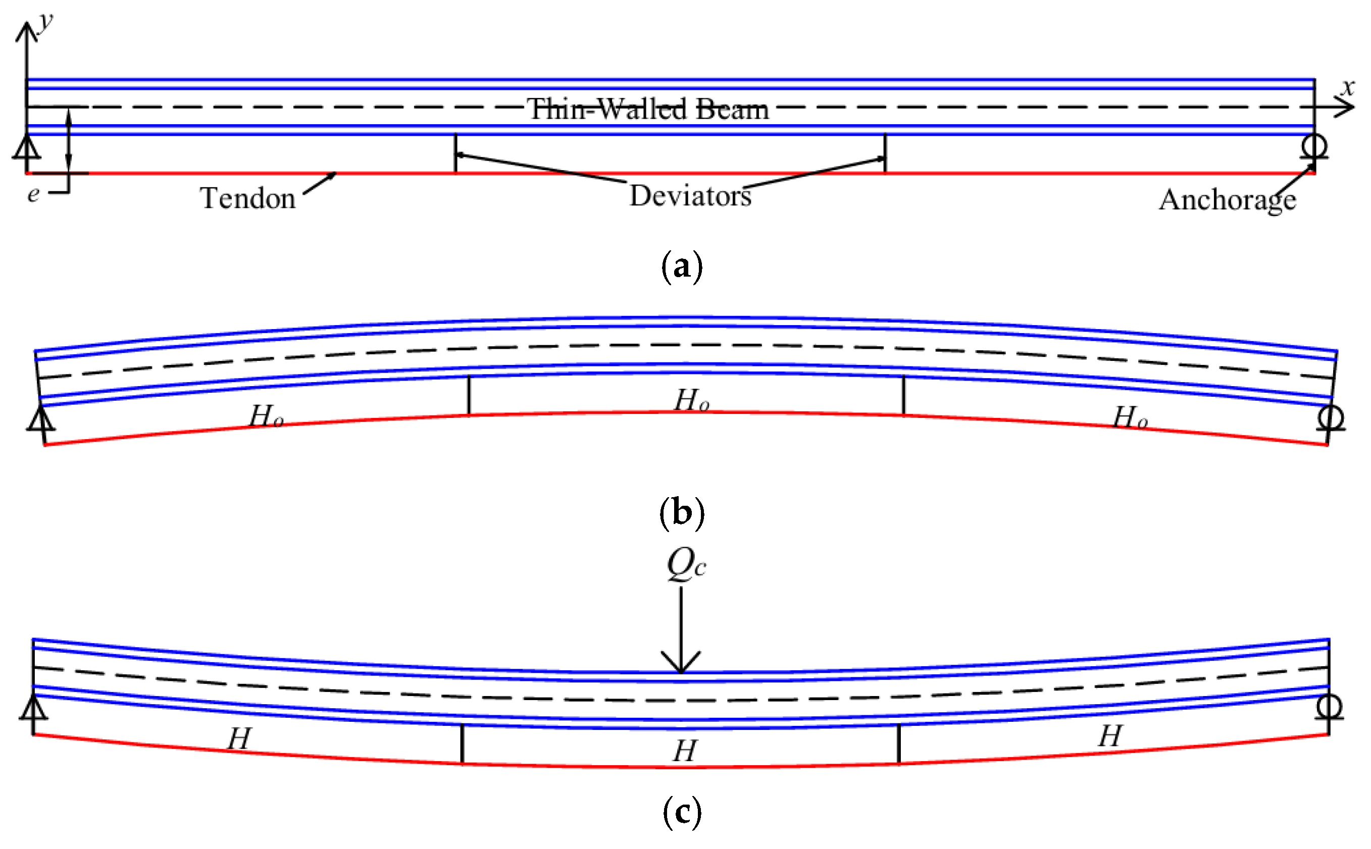
A bi-symmetric beam PS by a rectilinear tendon cable with discretely attached deviators are shown in Figure 1. It is assumed that the deviators are rigidly connected to the beam and encase the tendon under an un-bonded (i.e., allowing axially relative sliding) condition. Figure 1a exhibits a steel beam with two deviators and straight tendons prior to pre-stressing. Figure 1b depicts the deformed shape of the PS system under an initial pre-stressing force, Ho. Additionally, Figure 1c shows a PS beam possessing un-bonded deviators which have been subjected to a centrally lateral load, Qc.
To establish the stability theory of the PS system, the following assumptions were made: (i) all materials are linearly elastic and steel beam sections are bi-symmetric; (ii) since the deviators are rigidly fixed to the beam, the lateral movement of the tendons is entirely governed by the beam’s deformation at the contact points; (iii) at the initial stage of pre-stressing, the tendon force is uniformly distributed along the entire beam length; (iv) The deviator conditions are un-bonded, and discrete deviators are considered; (v) and lastly, in-plane flexural stiffness of the PS system is so large that in-plane member forces can be determined by linear elastic analysis due to external loads, and the effects of pre-buckling deformations are neglected.
Particularly, Figure 1a is considered to be the baseline configuration for the analysis. Using the compatibility condition illustrated in Figure 1b, a relationship between the unstrained tendon length, lc, and the initial pre-stress force, Ho, can be established [4]. The in-plane displacement components, u, and, v, account for the combined effects of initial pre-tension and external loading, while the out-of-plane displacements, w, and rotational deformation, θ, arise in the buckling state. Moreover, as illustrated in Figure 1c, a lateral load, Qc, applied either at the midpoint of simply supported beams or at two points, was used to capture the three-dimensional buckling behavior of PS systems subjected to non-uniform moment distributions. Note that the cable tension of H in Figure 1c remains unchanged along the tendon length, under the un-bonded condition. Designating the displacement components, u ,   v ,   w   , and twisting angle,   θ , along the centroidal axis of the beam, the geometrical boundary conditions of the simply supported beams can be given as:
u o = 0 = v o = w o = θ o   ;     v l = 0 = w l = θ l
where the prime = derivative with respect to x; u o = u ( 0 ) ;   v o = v ( 0 ) ;   θ l = θ ( l ) .

2.1. The Potential Energy of the PS Beam

The bi-symmetric thin-walled beams pre-stressed through a single tendon and subjected to the in-plane load, Qc, are taken into account where the axial force, F 1 A τ 11 d A , shear force, F 2 A τ 12 d A , and the bending moment, M 3 A y τ 11 d A , in the beams and tendon force, H, are generated due to Qc. Defining all of the displacement parameters, u ,   v ,   w   ,   θ , at the centroid, a potential energy expression of the thin-walled beams under lateral load Qc can be expressed as follows [38]:
Π B e a m = 1 2 0 l E A u 2 + E I 2 w 2 + E I 3 v 2 + G J θ 2 + E I ϕ θ 2 + F 1 v 2 + w 2 + β 1 θ 2 + F 2 w θ + M 3 w θ w θ d x + Q c v ( l / 2 )
where EA, EI2, EI3, GJ, EIφ represents the axial, flexural, torsional, warping rigidities of the beam and β 1 = I 2 + I 3 / A respectively; note that the M 3 should be understood as a semi-tangential moment.
Referring to [23], the potential energy of the straight tendon with discretely attached m-1 un-bonded deviators are expressed as:
Π T e n d o n = E A c 2 l c l l c + u l u o + v l v o e 2 + H e 2 θ l w l θ o w o + H 2 i = 1 m v i q v i p 2 l i   + w i q θ i q e w i p + θ i p e 2 l i    
where m is the total number of tendon segments; l ,   l c ,   l i represents the beam length and unstrained tendon length of tendon and ith tendon segment length, respectively;   v i p , v i q and θ i p , θ i q correspond to the vertical displacements and twisting angles at left and right ends of the i t h tendon segment. The total potential energies of the PS beams by summing Equations (2) and (3), possessing discreet un-bonded deviators, can be expressed as follows (Mehdi et al. [39]):
Π P S = Π B e a m + Π T e n d o n Π P S = 1 2 0 l E A u 2 + E I 3 v 2 + E I 2 w 2 + E I ϕ θ 2 + G J θ 2   + F 1 v 2 + w 2 + β 1 θ 2 + 2 F 2 w θ 2 M 3 w θ d x + E A c 2 l c l l c + u m q u 1 p + v m q v 1 p e 2 + H 2 i = 1 m 1 l i v i q v i p 2 + w i q θ i q e w i p + θ i p e 2 + Q v ( l / 2 )
The total potential energies of Equation (4) can be separated into in-plane and out-of-plane energy terms as follows:
Π P S I n = 1 2 0 l E A u 2 + E I 3 v 2 + F 1 v 2 d x + Q v ( l / 2 )                             + E A c 2 l c l l c + u m q u 1 p + v m q v 1 p e 2 + H 2 i = 1 m 1 l i v i q v i p 2 Π P S O u t = 1 2 0 l E I 2 w 2 + E I ϕ θ 2 + G J θ 2   + F 1 w 2 + β 1 θ 2 + 2 F 2 w θ 2 M 3 w θ d x                               + H 2 i = 1 m 1 l i w i q θ i q e w i p + θ i p e 2

2.2. Approximate Solution of PS Beams Using Rayleigh–Ritz Method

In the case of the spatial buckling problem for PS beams with one deviator under uniform bending, the exact solutions have been presented in a closed form by Kim et al. [21]. However, it is clear that the exact solutions become extremely complicated with the increase in deviators. So, approximate solutions using Rayleigh–Ritz method are provided in this section.
When obtaining the generalized out-of-plane buckling solution for a PS beam with multiple deviators, as shown in Figure 2, the beam was modeled with m 1 deviators positioned at regular intervals along its span. These deviators divide the beam into equal segments, resulting in a segmented tendon length as Δ l = l / m . Equation (6) is presented from Equation (5), which describes the out-of-plane buckling behavior of a PS beam with m 1 deviators as follows:
Π P S O u t = 1 2 i = 1 m 0 l i E I 2 w i 2 + E I ϕ θ i 2 + G J θ i 2 + F 1 w i 2 + β 1 θ i 2 + 2 F 2 w i θ 2 M 3 w i θ i d x + H 2 i = 1 m 1 l i w i q θ i q e w i p + θ i p e 2
Especially in this study, only PS beams subjected to lateral load, Qc, were considered. The internal forces in the beams under un-bonded conditions reported by Mehdi et al. [39] can be expressed as follows:
F 1 = H ,   M 3   =   e H + Q c M Q ,   F 2 = Q c M Q ,   H = H o + C Q Q c where               C Q = e l 8 E A c + H o E I 3 + E A c e 2 + I 3 / A
Now, the Ritz process of solving the LTB problems of the PS beams based on Equation (6) can be given as follows:
Step 1: Introduce the harmonic functions as the admissible functions of w, θ.
w = k = 1 5 A k sin k π x l   ,   θ = k = 1 5 B k sin k π x l
Step 2: Substitute the admissible functions defined in Equation (8) into the energy expressions from Equation (6), and then integrate them.
Step 3: Obtain the out-of-plane equilibrium equations by invoking the stationary principle:
Π P S O u t A k = 0   ,   Π P S O u t B k = 0   for   k = 1 , 2 , 5
Step 4: Obtain a stability equation by taking the determinant of the linear equations and determine the critical buckling loads or critical moments of simple PS beams depending on the number of deviators.
A symbolic calculation has been extensively used in the integration of Equation (6), calculating the linear equilibrium equations and determining the critical loads by setting a determinant of them equal to zero. Generally, more accurate solutions can be expected by including as many terms as possible in Equation (8). To evaluate the first critical load, buckling equations have been derived by considering one term only k = 1 , and the resulting quadratic equations in terms of Qc are expressed as:
det 8 E I 2 π 4 8 l 2 H π 2 G l 2 8 e H π 2 l Q c 4 + π 2 + e G l 2 8 e H π 2 l Q c 4 + π 2 + e G 8 π 2 E I w π 2 + l 2 G J β 1 H e 2 G = 0                   G = 16 H l 2 1 + m 2 cos π 1 + m 1
Notably, the analytical solution for two or three terms becomes more complex to be provided, so only one-term solution is presented in Equation (10). The numerical solution of one, two and five terms are given in Table 2.

3. FE Modeling of PS Beams

The purpose of conducting detailed numerical simulations using FE analysis software ABAQUS [40] is to investigate the LTB behavior of externally PS thin-walled steel beams under one-point and two-point vertical loadings. These simulations are essential due to the lack of design code provisions, and the analytical approach to obtain the exact solutions for such systems is either not available or can be extremely complicated [21,23], as the resulting differential equations contain variable coefficients particularly under non-uniform bending. Although an approximate analytical solution based on one-term Rayleigh–Ritz method is introduced in Section 2 for centrally loaded beams, it does not adequately predict LTB loads. Therefore, FE models are first developed to verify the approximate analytical solution against the one-point (central) loading case. Once validated, the developed FE models are subsequently employed for two-point loading case and compared with the experimental results. Accordingly, this adopted step-by-step validation strategy ensures consistency between the analytical, FE-based numerical and experimental investigations to serve as a reliable basis for performing parametric studies and generating a comprehensive dataset under varied geometric and pre-stressing conditions. The detailed modeling procedures, assumptions, and validations are presented in Section 3.1, Section 3.2 and Section 3.3, while a parametric study is conducted in Section 3.4 to examine the influence of key geometric and pre-stressing variables on the LTB capacity of externally PS steel beams.

3.1. Development of FE Models

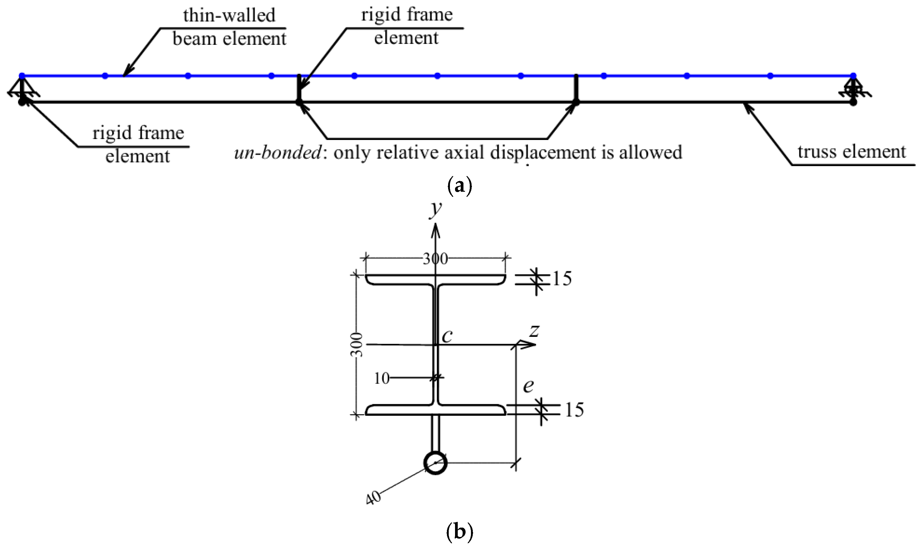
The geometry of the PS I-beam system investigated is defined using a bi-symmetric thin-walled I-section. The tendon includes rectilinear cables placed eccentrically from the centroid and guided through deviators located along the beam span. Figure 3b shows the bi-symmetric cross sections, and Table 1 lists their material and geometric properties which have been calculated based on the centroid formulation [38]. The thin-walled I-beam is modeled using B32OS elements in ABAQUS [40], which possess seven degrees of freedom per node and can capture flexural, torsional, and warping deformations critical for LTB behavior. The tendon elements are defined as truss elements (T3D2) capable of carrying axial force only and are un-bonded between deviators and anchorages. Very stiff frame elements (B32) are used to model deviators and anchorage points and are assigned high axial and flexural stiffness (2.589 × 10¹³ kN and 2.589 × 10¹³ kN·mm2, respectively) to act as rigid constraints without influencing the global behavior of the system.
The pre-stressing force, Ho, in the tendon is introduced using the thermal loading technique. The thermal loading is determined using l l c = α   T l c , where α is coefficient of thermal expansion, T is thermal load, and l c are the unstrained lengths of tendon segments, which have been analytically derived by Kim et al. [4]. Figure 3a shows a FE model of a pre-stressed beam system consisting of thin-walled beam elements for the steel beam, very stiff frame elements rigidly connected to the beam for the anchorage/deviators, and truss elements for the tendon segments. The un-bonded contact conditions between the deviator and cable are used for the modeling of tendon segments.
The stability analysis of the PS beam is carried out in two sequential steps. In the first step, Ho is introduced into the tendon system under a general linear analysis, producing the initial stress state and deformation pattern of the beam; this condition is shown in Figure 4, which illustrates the beam deformed only under the constant pre-stress force. In the second step, a buckling analysis is conducted on the PS system by applying a unit load to trigger LTB behavior; this is illustrated in Figure 5, where the beam is subjected to one-point (central) and two-point vertical loadings denoted as Qc and Qp = 1 kN. By keeping external load as a unit load, the FE model can extract buckling load factors, which are later scaled to represent real loads. Through this two-step procedure, the influence of pre-stressing on the LTB response can be appropriately captured.

3.2. Validation of FE Models

The developed FE models are validated against a series of approximate analytical solutions derived for centrally loaded PS steel beams. Since no closed-form analytical solution exists for two-point loading condition due to the complexity of moment distribution and pre-stressing interaction, the validation is limited to the one-point (central) load case. To this end, Ritz solutions using one-, two-, and five-term functions are computed to assess the convergence behavior and to provide reference values for model verification.
Table 2 presents a comparative summary of the LTB loads obtained from the analytical Ritz solutions and the FE simulations conducted in ABAQUS [40] under Ho = 400 kN and e = 220.0 mm. The one-term Ritz solution provides a simplified approximation of the buckling resistance and represents a conservative lower-bound estimate. As more terms are included in the Ritz expansion, the accuracy improves considerably, with the five-term result converging towards the FE solution. A close agreement between the ABAQUS simulations and the higher-order Ritz solutions confirms the validity of the FE modeling approach for simulating the LTB behavior of externally PS steel beams. Overall, the results demonstrated that the developed FE models are capable of reliably simulating the LTB response of PS steel beams under one-point (central) loading and can be extended to more complex configurations where there is a lack of analytical solutions and design codes.

3.3. Validation of FE Modeling via Experimental Testing

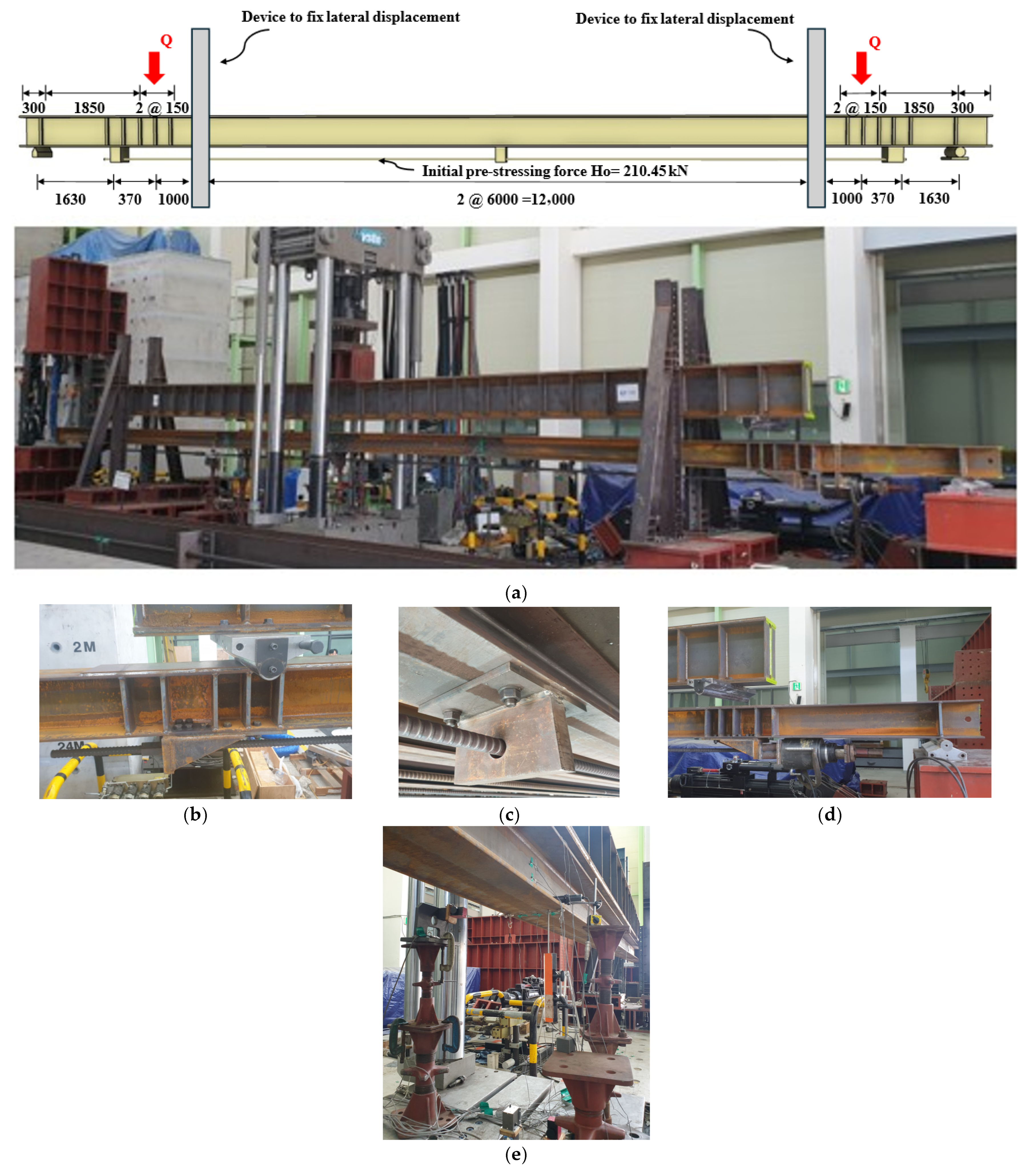
The experimental data reported by Kim et al. [25] are presented in this study to validate FE models. A hot-rolled steel beam (H-300 × 305 × 15 × 15) of SM355 grade, externally pre-stressed with a Dywidag thread bar (diameter = 40 mm), was selected for the tests. The experimental setup, featuring a simply supported pre-stressed (PS) steel beam under two-point loading, is shown in Figure 6a. This setup includes a steel H-beam, a device for constraining lateral displacement, and a tendon bar externally attached via rigid anchorage before pre-stressing. The eccentricity of the PS tendon bar is 280 mm from the centroid of the H-beam, and the tendon bar’s diameter is 40 mm. To prevent local buckling of the steel beam, vertical stiffeners (t = 20 mm) were welded at the tendon anchorage points and vertical loading points along the PS beam. A pre-stressing force of 210.45 kN was applied to the tendon bar using a 1000 kN hydraulic jack. The experiments were carried out at the Hybrid Structural Testing Center of Korea Construction Engineering Development. Special lateral bracing was implemented to ensure complete lateral support, preventing displacement and torsional rotation, as shown in Figure 6a. The schematic of the tendon bar’s fixed anchorage, un-bonded mid-span deviator at the bottom flange of the H-beam, and pre-stressing anchorage are depicted in Figure 6b–d. Notably, the experimental configuration shown in Figure 6 was employed to validate the accuracy of the proposed FE modeling approach in capturing the governing LTB mechanism of externally pre-stressed steel beam under non-uniform bending. Accordingly, the comparison between the experimental results and FE modeling was performed at the level of global instability behavior and load–displacement response rather than direct numerical equivalence. This provides a reliable basis for subsequent parametric studies and ML dataset generation.
The specimens were simply supported and loaded by two-point vertical loading via a very stiff loading beam subjected to a vertical load as shown in Figure 6a. The length of the loading beam was 15 m and the distance between the two vertical loads was 14 m. The cross-section of the loading beam was H-588 × 300 × 12 × 20, and two cover plates (L = 15 m, t = 20 mm) were welded at the top and bottom flanges. In addition, the vertical stiffeners (t = 20 mm) were welded at every 500 mm along the web. The lateral restraints shown in Figure 6a were employed to provide an intermediate unbraced length of 12 m. Importantly, these lateral restraints were not intended to suppress the lateral stability but rather to prevent premature global collapse and to ensure safe and controlled experimental execution. This is supported by the experimental results which showed that the steel beam still exhibited the global LTB deformation under non-uniform bending.
The load data were measured and automatically collected by the MTS loading system. LVDTs and strain gauges were used to measure the deflection and strain data of the specimens. The lateral displacement at the end of the lower flange and two vertical displacements at both sides of the lower flange were measured using the potentiometers installed at the mid-span of the beams, as shown in Figure 6e. The load data were measured and automatically recorded by the MTS loading system. LVDTs and strain gauges were used to measure the deflection and strain responses of the specimens. The lateral displacement at the end of the lower flange and the two vertical displacements at both sides of the lower flange were measured using potentiometers installed at the mid-span of the beams, also shown in Figure 6e.
The two rigid end anchorage supports were fixed to the lower flange using high-strength bolts, as shown in Figure 6b,d. The tendon bar was connected to both the fixed-end and loading-end anchorages, and a hydraulic jack was used to apply the pre-stressing tensile force, as illustrated in Figure 6d. After tensioning the tendon bar, the nuts of the connecting screws were fully tightened. During the tensioning process, the tensile strain of the tendon bar was monitored using strain gauges bonded directly onto the bar. Direct tensile tests were performed to verify the material properties of the steel H-beam and tendon bar. Three H-beam specimens and two tendon bar specimens were tested, using the same 40 mm-diameter tendon bar applied in the PS beam. The tendon bar exhibited an almost linear tensile stress–strain response. The mean yield stresses were 355 MPa for the H-beam and 1000 MPa for the tendon bar. These properties were subsequently used as input material parameters in the finite element model for comparison with the experimental results. Furthermore, based on these yield stress values, the plastic moment capacity of the experimental specimen is calculated as 837.7 kN·m using the analytical expression presented in Appendix A.
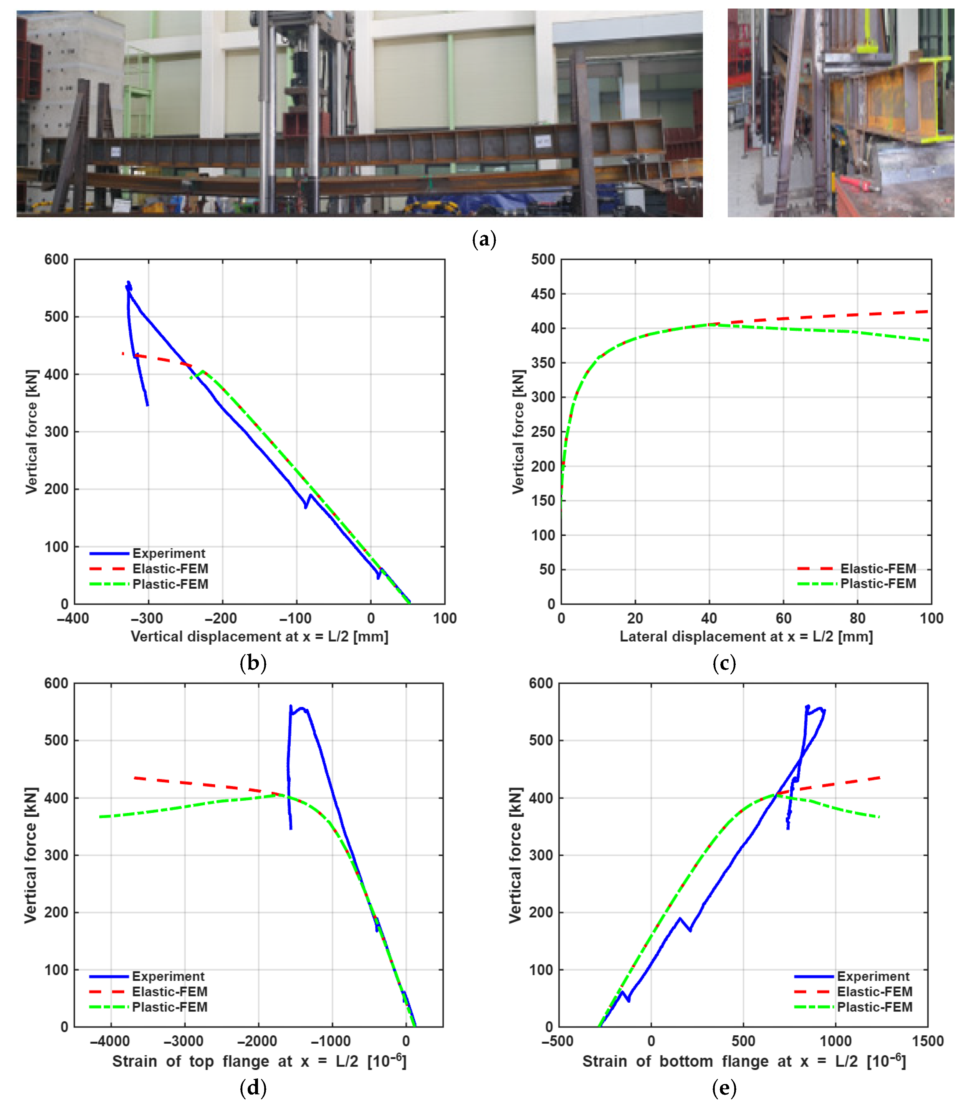
In the initial stage, a pre-stressing force of 210.45 kN was applied to the tendon bar, inducing an upward in-plane deflection of the PS beam. As vertical load was applied, the in-plane downward deflection increased linearly with the load. As the maximum load approached, the lateral displacement and torsional rotation gradually increased, leading to LTB, as shown in Figure 7a. Local buckling did not occur before reaching the maximum load. The experimental results were compared with numerical simulations using elastic and elastoplastic material models in ABAQUS, as shown in Figure 7. The non-linear FE modeling was conducted using two sequential analysis steps. First, an elastic eigenvalue buckling analysis was performed to identify the LTB mode shapes and corresponding elastic critical buckling loads. Notably, these elastic critical buckling loads are used to characterize the elastic LTB resistance and form the basis for subsequent parametric investigations and ML dataset generation. As such, they are intended to represent the elastic stability criteria rather than ultimate strength or post-buckling capacity. Second, a non-linear static analysis based on the Riks method was carried out to obtain the full load–displacement response, accounting for both geometric and material non-linearities. In this step, the LTB mode shape obtained from the elastic buckling analysis was introduced into the model as an initial geometric imperfection. In the experiment, the initial imperfection of the PS beam measured and presented by Kim et al. [25] was directly applied to the numerical model. The initial twist and local geometric defects were not measured and were therefore not included. Residual stresses were also neglected in the numerical simulations. The elastic material model was employed in the eigenvalue buckling analysis, while an elastoplastic material model without strain hardening was adopted in the non-linear Riks analysis.
Two numerical curves were obtained: one based on an elastoplastic material model (“Plastic-FEM”) and the other on an elastic material model (“Elastic-FEM”). The experimental results showed good agreement with both numerical approaches. Displacement and strain measurements from the experiments closely matched the numerical results.

3.4. Parametric Studies

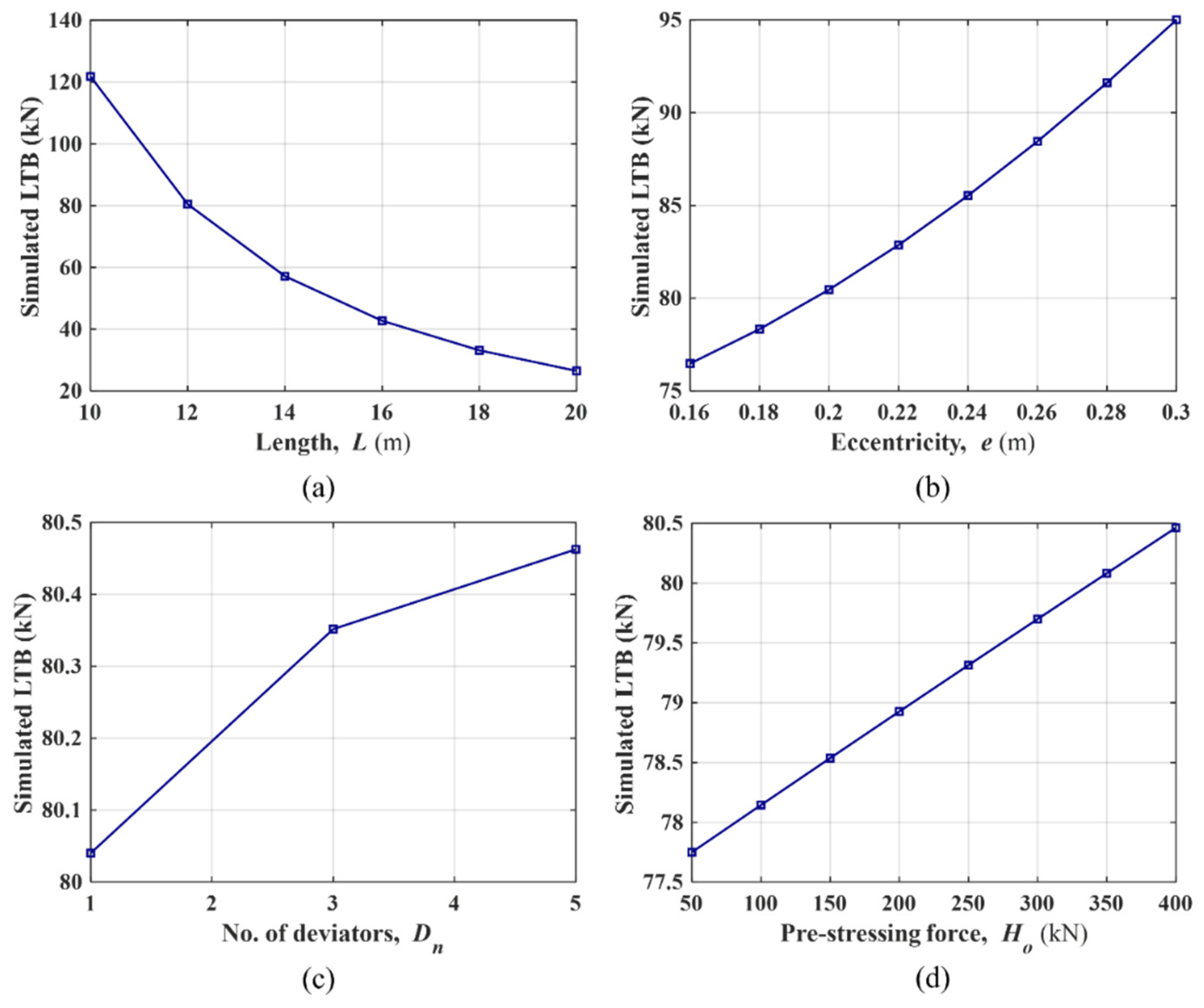
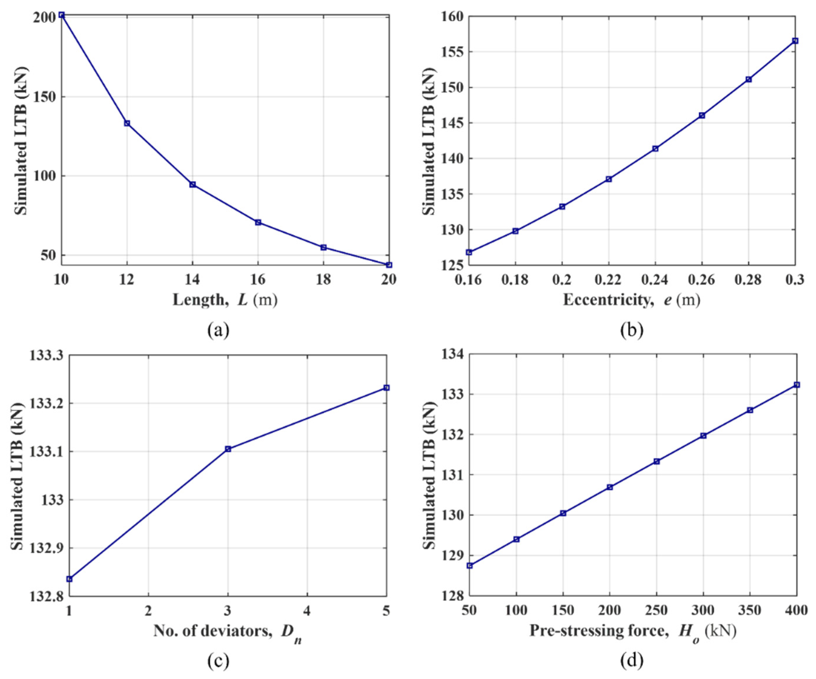
A parametric study is further conducted to examine the influence of key variables on the LTB capacity of externally PS steel beams. Four key parameters, including geometric and pre-stressing variables were considered: the unstrained span length L (10 m to 20 m) of the beam, the eccentricity e (0.16 to 0.3 m) of the tendon, the number of deviators Dn (1 to 5), and the applied pre-stressing force Ho (50 to 400 kN). These parameters were selected because they directly govern the pre-stressing-induced stiffness modification and the global stability behavior of the PS system. Notably, the influence of other parameters such as cross-sectional geometry and material properties on the LTB behavior has been extensively investigated and is well-captured by the classical beam stability theory and current design codes. Accordingly, these parameters were kept constant to isolate the combined effects of pre-stressing force, tendon eccentricity, and deviator configuration on the LTB resistance of PS steel beams under non-uniform bending, which remain insufficiently explored. To do so, one parameter in each case was varied, while the others were kept constant to show its effect on the buckling response. The results show that the LTB capacity decreases with increasing L, reflecting the higher slenderness associated with longer spans. In contrast, an increase in e, Dn, or Ho leads to a corresponding increase in LTB resistance, as these factors enhance the stabilizing influence of the pre-stressing system. The trends of these parametric variations for one-point (central) and two-point loadings are illustrated in Figure 8 and Figure 9, which clearly demonstrate the relative sensitivity of the LTB response to each parameter.

4. Machine Learning (ML) Approaches

The model-based numerical analysis techniques such as FE simulations considering complex PS structural systems are quite computationally intensive and time-consuming, requiring extensive expert calibration and often relying on expensive commercial software like ABAQUS [21,33,39,41]. As a result, their direct applications becomes impractical for large-scale parametric studies, optimization, and preliminary design stages requiring thousands of structural configurations. In contrast, data-driven ML approaches offer promise in overcoming the shortcomings of the model-based approaches by utilizing statistical data instead of FEM to effectively simulate the structural behavior [32,33,34]. These data-driven ML models efficiently capture the complex input–output relationships of the structural system without knowing the extensive prior knowledge of the structural behavior. In this study, ML is employed as a computationally efficient surrogate modeling framework trained on validated FE-based dataset, enabling reliable and fast prediction of LTB capacity across a wide range of practical PS beam configurations. Accordingly, several ML models are investigated by employing the key geometric and pre-stressing variables as critical influencing parameters to predict the LTB capacity of the externally PS steel beams. In particular, support vector regression (SVR), random forest (RF), and least-square boosting (LSBoost), representing prominent techniques from distinguished families of support vector machines and decision trees, as reported in the recent related studies [35,36,37,42,43], are employed as data-driven ML models. These models are widely recognized for their robustness, flexibility, and ability to efficiently capture complex non-linear relationships within datasets, making them well-suited for simulating and predicting structural behaviors such as LTB capacity of the PS steel beams. However, the optimal performance of the considered ML models necessitates careful tuning of their corresponding training parameters to enhance the generalizability and prediction accuracy [34,35,42,44]. To achieve this, ML models employed in this study are integrated with Bayesian optimization (BO), a powerful probabilistic algorithm for robust hyperparameter tuning [45,46,47]. The following sub-sections provide a concise overview of each data-driven ML model and implementation of BO for hyperparameter tuning considered in this study.

4.1. Support Vector Regression (SVR)

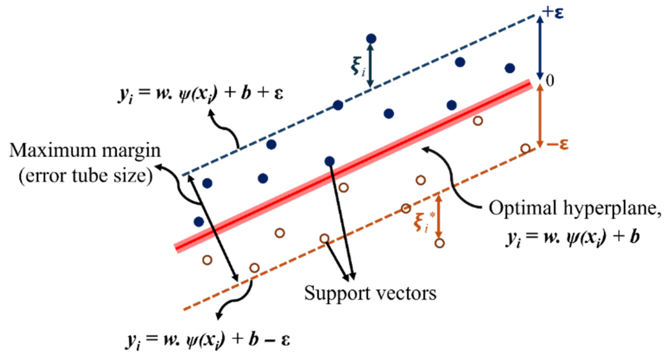
SVR is an extension of support vector machines, a robust and widely used supervised ML model for classification, regression, and pattern recognition tasks. Support vector machines was initially introduced by Vladimir Vapnik in the 1960s and later formalized by Boser in 1992 for classification with non-linear classifiers [48,49]. SVR extends the principles of support vector machines to regression problems, enabling the prediction of continuous target values [50]. It employs kernel functions, such as the radial basis function used in this study, to transform input data into a higher-dimensional feature space, where it constructs a hyperplane to minimize the loss function. Figure 10 illustrates the mechanism of the SVR. The process involves three main steps: (i) mapping the input space to a feature space using kernels; (ii) constructing a hyperplane in the feature space by solving an optimization problem; and (iii) modifying the loss function to quantify errors between predicted and actual outputs [36,37,51]. Note that the complexity and accuracy of the SVR model rely on the key data points called support vectors, which determine the optimal position and orientation of the hyperplane [35,50]. The effectiveness and adaptability of SVR, combined with its reliance on support vectors, make it particularly suitable for accurate modeling of complex non-linear relationships between the influencing parameters and structural behaviors.

4.2. Random Forest (RF)

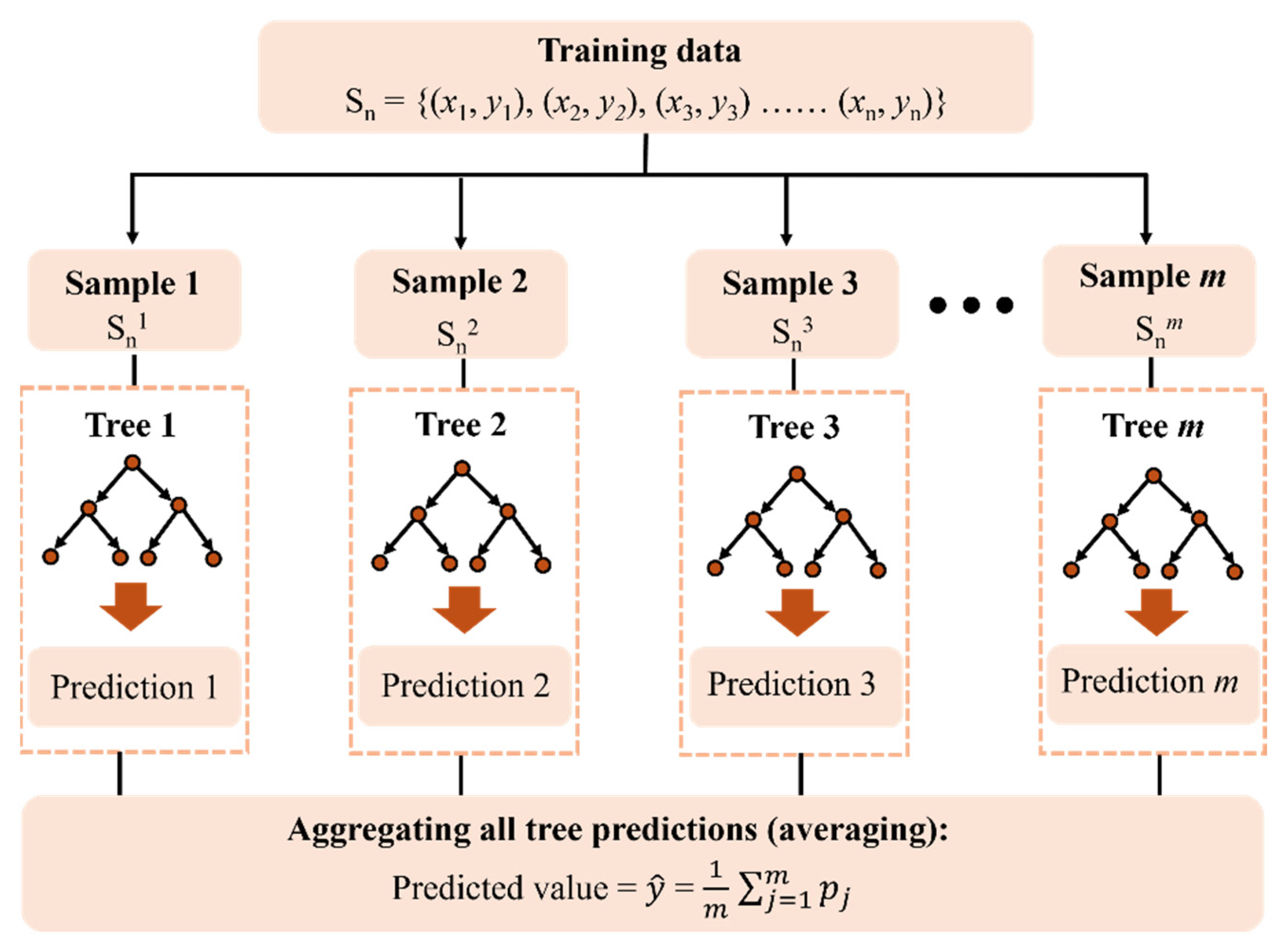
RF algorithm introduced by Breiman [52,53] is a popular ensemble learning technique that utilizes individual decision trees as weak learners for both classification and regression tasks, with the trees typically trained through bootstrap aggregating (bagging). In the context of regression tasks, as employed in this study, the decision trees in RF are constructed independently as an ensemble, and their predictions are aggregated through averaging, resulting in a more robust and accurate data-driven ML model. Additionally, RF is capable of handling both numerical and categorical data with minimal preprocessing and performs well on large datasets with numerous input variables [35]. Figure 11 depicts the schematic of the RF algorithm. The main steps of the RF algorithm include: (i) creating multiple bootstrap samples from the original dataset, where some data points may appear multiple times, while others may be excluded; (ii) training a decision tree on each bootstrap sample using a randomly selected subset of features at each split, which reduces correlation between the trees; and (iii) aggregating the predictions from all decision trees through averaging to produce the final output [36,37,42]. The inherent randomness in RF reduces the overfitting while enhancing generalizability, enabling the ensemble approach to improve the model performance in decision-making process.

4.3. Least-Square Boosting (LSBoost)

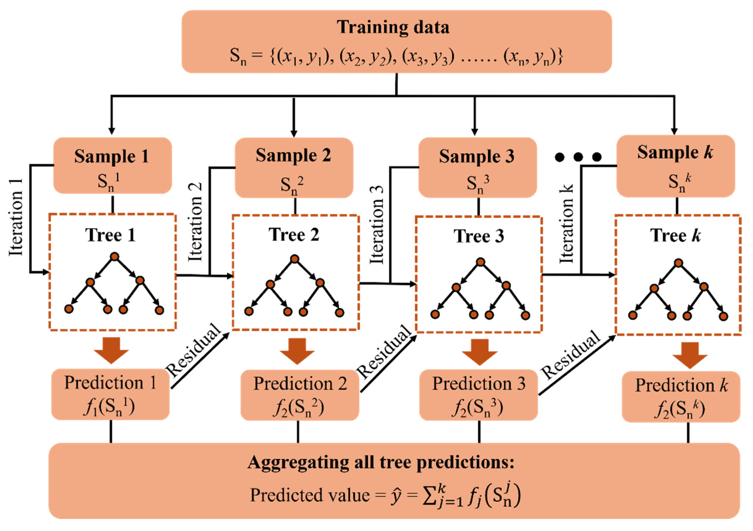
The LSBoost algorithm, introduced by Friedman [54], is a widely used gradient-boosting technique that builds an ensemble of weak learners, typically decision trees, to produce a strong learner for enhancing the predictive performance of a data-driven ML model [43]. LSBoost is well-suited for regression problems, with its capability to model complex non-linear relationships in datasets and effectively handle large datasets, as well as missing data. In LSBoost, weak learners are trained sequentially, with each subsequent learner minimizing the residual errors of previous learners using the least-squares loss function. This iterative process combines the boosting algorithm with gradient descent, an optimization algorithm that ensures that the model gradually converges to an optimal solution by reducing the prediction error at each step [43,54]. Figure 12 illustrates the schematic of the LSBoost algorithm. The primary steps of the LSBoost algorithm include: (i) initializing the model with a constant value, typically the mean of the target variable; (ii) iteratively fitting weak learners, where each learner models the residual errors of the previous model; (iii) updating the ensemble by adding the predictions of the new learner, scaled by a learning rate to control overfitting and improve generalizability; and (iv) aggregating the contributions of all learners to produce the final model [37,43,55]. The iterative refinement approach of the LSBoost algorithm ensures accurate and robust predictions, making it a reliable ML model in data-driven applications.

4.4. Hyperparameter Tuning of ML Models Using BO

The effectiveness and accuracy of the adopted ML models are significantly influenced by their parameters, commonly known as hyperparameters, which govern their training processes and avoid overfitting or underfitting. Consequently, improving the predictive performance (i.e., generalizability) of considered ML models requires the careful selection of their training hyperparameters [35,42,43]. Nonetheless, there is no consensus on the most effective approach for hyperparameter selection. A commonly used approach to fine-tune the ML hyperparameters is the trail-and-error, grid-, and random-search optimization methods [35,42,56], which involve examining various combinations of hyperparameters to identify the optimal parameter configuration. Despite their effectiveness, these methods are computationally intensive and time-consuming due to many ML hyperparameters having coupling effects within a vast search space [47,56]. Therefore, a more efficient and robust optimization method is necessary.
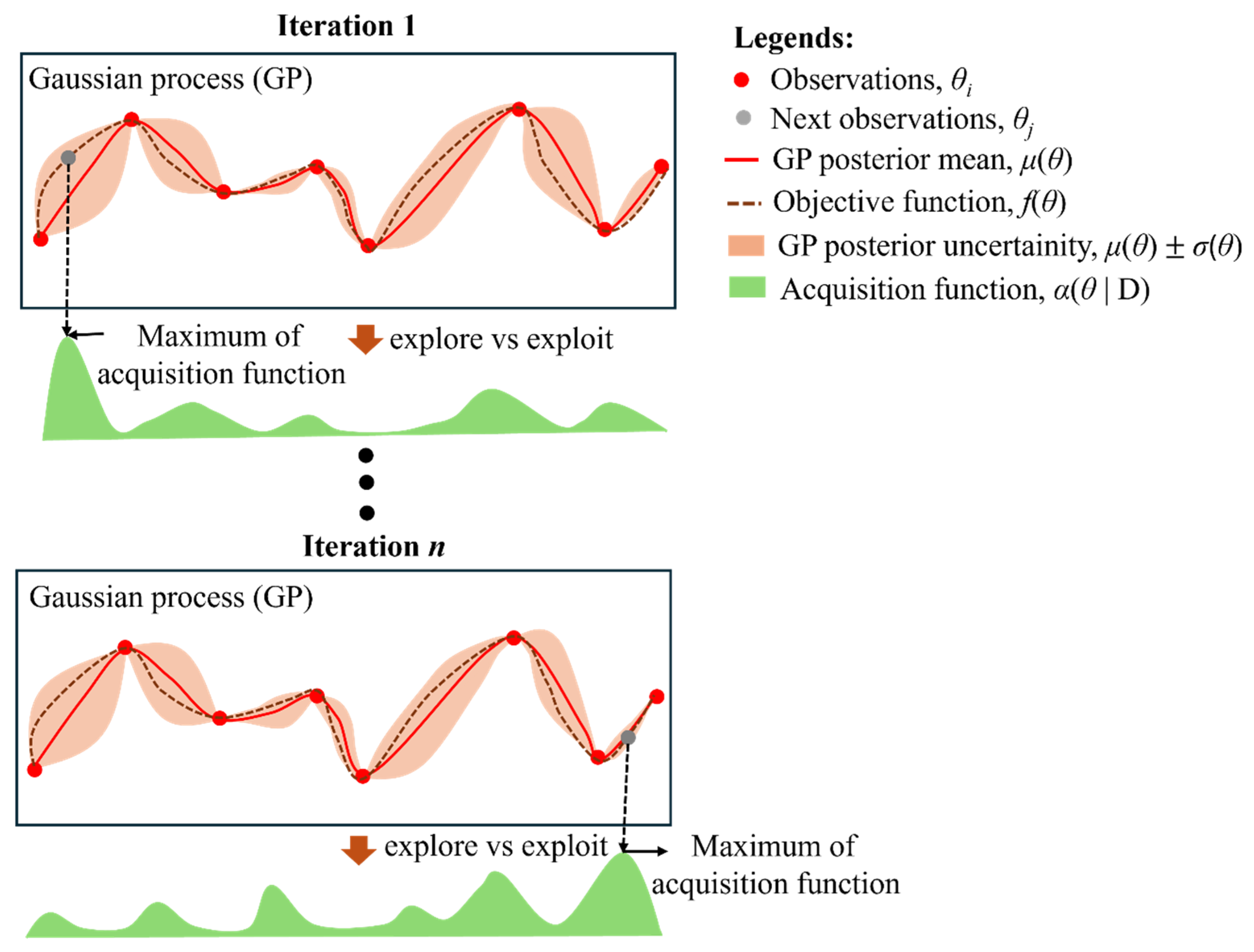
BO has emerged as a powerful technique for ML hyperparameter optimization, effectively overcoming the limitations of the conventional trial-and-error, grid-, and random-search methods [46,47,56]. BO employs an underlying Gaussian process model [45], as shown in Figure 13, making it particularly well-suited for the global optimization of black-box objective functions that are difficult to evaluate. By leveraging prior distributions and sample data, BO explores the posterior distribution of the objective function. In BO, the loss of the ML model is typically defined as the objective function of the hyperparameters, and BO systematically searches for its global minimum based on the Gaussian process prior. An acquisition function is then employed to guide the search process by iteratively determining the next set of hyperparameters to evaluate by maximizing acquisition function over the Gaussian process. Thus, the ability of BO to identify the promising regions by balancing the exploration of uncertain areas with exploitation of known high-performing region requires fewer iterations to determine the optimal parameter configurations, making BO more efficient and faster than conventional methods [47,56]. Therefore, ML approaches are integrated with BO in this study to build robust and accurate data-driven models incorporating the pre-stressing and geometric parameters for predicting the LTB capacity.

5. Application, Evaluation, and Interpretation of BO-ML Approaches

5.1. Dataset Preparation

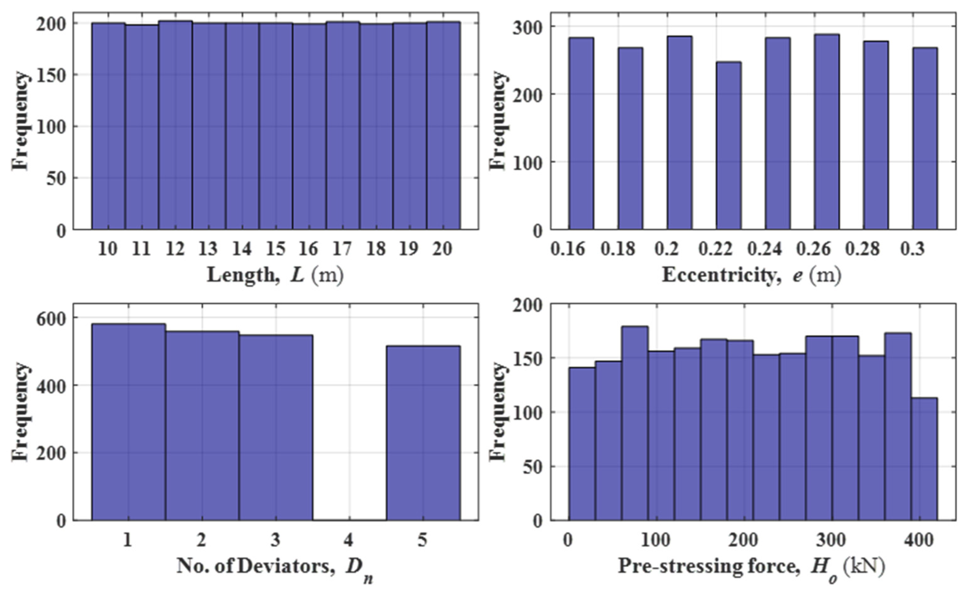
The proposed study investigates the performance of the aforementioned data-driven ML approaches in predicting the LTB capacity of the PS steel beams. To facilitate this, a comprehensive dataset was constructed based on the FE simulations, as discussed in Section 3, by compiling the input parameters that predominately govern the LTB behavior of the PS steel beams under non-uniform bending from one-point (central) and two-point loadings for bi-symmetric section. These parameters include the key geometric and pre-stressing variables, identified as critical influencing factors governing the LTB response. Figure 14 illustrates the range and distribution of the input parameters used for training the ML models. Herein, a total of 2200 input datapoints were utilized to simulate the LTB capacity of PS steel beams. Notably, this diverse range of input parameters was carefully selected to ensure the generalizability of the ML approaches across the practical PS steel beam configurations for predicting the LTB resistance under both central and two-point loading conditions.
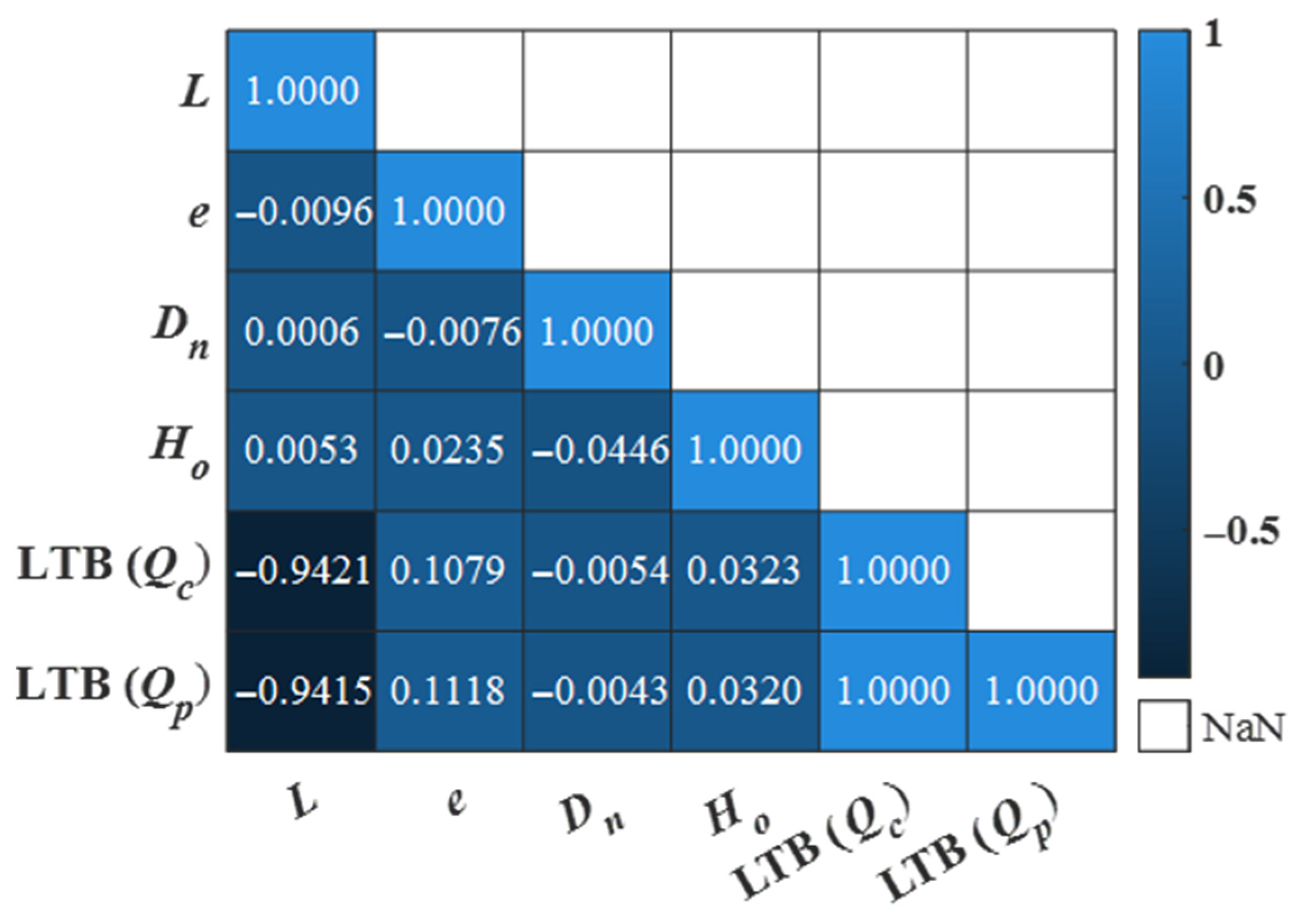
Feature engineering is one of the essential steps in dataset preparation to ensure the efficient performance of the data-driven ML approaches. It involves identifying and eliminating the redundant input parameters while retaining those that contribute meaningful information, resulting in ML models that are more accurate, robust, and interpretable [56,57]. In this study, multicollinearity was adopted as a criterion for feature selection, as its existence can impede the model’s capacity to capture meaningful information and thus affect the predictive accuracy. In this regard, it is recommended to eliminate the highly correlated input features to overcome the issues related to multicollinearity, as well as overfitting [57,58]. Therefore, the Pearson correlation analysis was employed to evaluate the multicollinearity of input features using correlation coefficient (R-value), as illustrated in Figure 15. The selected input parameters (i.e., L, e, Dn, Ho) exhibited collinearity values close to zero, indicating a very low degree of interdependence. Consequently, all the input parameters were retained to ensure their effectiveness in modeling the LTB capacity with ML approaches. Additionally, as depicted in Figure 15, the collinearity between the input parameters and target variables (i.e., LTB capacity under one point (central) and two-point loading conditions) was generally low, with most R-values for the pre-stressing parameters ranging from 0 to 0.15, except for span length L, which exhibited a strong correlation (R > 0.90). As such, this further justifies the selection of ML approaches capable of modeling non-linear relationships between the input and target variables.
Following the feature engineering, the dataset containing the input parameters and target variables was divided into training (80%) and testing (20%) subsets. The testing dataset was kept unseen during the training of the ML models to ensure an unbiased performance evaluation. To facilitate efficient training process, the training and testing datasets were normalized to a uniform scale [−1, 1] using the min–max normalization technique [47,56]. This normalization approach eliminates the dimensional effect of the input parameters on the target variables, thereby enhancing the convergence speed, stability, and accuracy of the ML models during the training process.

5.2. Implementation of BO for Hyperparameter Tuning

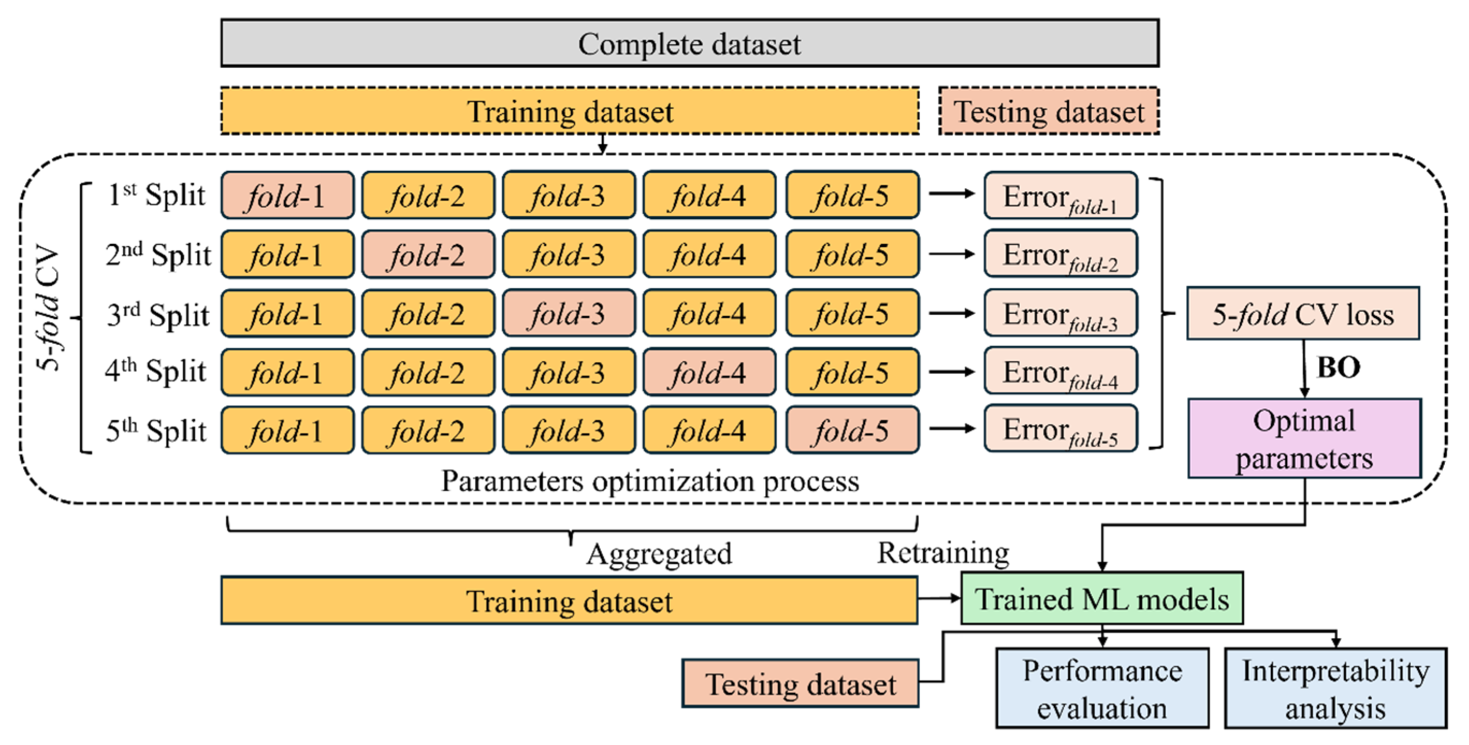
To optimize the parameters of the adopted ML approaches (i.e., SVR, RF, and LSBoost) via BO, the cross-validation technique was utilized to reliably evaluate the model performance during the hyperparameter tuning process. This technique helps to mitigate the bias associated with the random sampling of the training dataset and offers a more generalized estimate for determining optimal ML parameters [59]. In this study, a k-fold cross-validation technique was adopted, wherein the training dataset was partitioned into k mutually exclusive folds. The models were trained and validated k times, each time using k-1 folds for training and the remaining fold for validation, ensuring that every datapoint contributed to both training and validation exactly once. Figure 16 illustrates the overall framework utilized in this study for hyperparameter tuning of the SVR, RF, and LSBoost models using BO. Herein, the five-fold cross-validation loss [56], computed as the average root mean error (RMSE) shown in Equation (11), was used as an objective function, f(θ), in BO to determine the optimal parameters.
f θ = 1 5 f o l d = 1 f o l d = 5 R M S E f o l d
where RMSEfold represents the error calculated on the left-out validation fold using Equation (11). Notably, once the optimal parameters based on five-fold cross-validation loss were determined, the partitioned training dataset was recombined into a single dataset to retrain the adopted ML approaches with their respective optimal parameters, thereby enabling the evaluation of generalizability and predictive accuracy on the completely unseen testing dataset. The overall framework for integrating the ML models with BO for hyperparameter tuning was programmed in MATLAB R2025b on a PC equipped with an Intel Core i5 (12th Gen)-12450 processor and 16 GB of RAM.
Table 3 summarizes the optimal hyperparameters obtained for SVR, RF, and LSBoost within their respective tuning search spaces, using BO for LTB resistance as target variable under central one-point (Qc) and two-point (Qp) loading conditions. As shown in Table 3, the models exhibited distinct optimal configurations under different loading conditions, reflecting their adaptability to varying structural response complexities. For instance, the BO-SVR model yielded near-stable optimal values across both loading cases, with a slight increase in the regularization constant and a decrease in the kernel scale under the Qp condition, implying a modest increase in flexibility with a more localized kernel to better capture the inherent response complexity. Similarly, the BO-LSBoost model employed slightly more boosting iterations and a greater maximum tree depth, together with a higher learning rate (i.e., reduced shrinkage) under the Qp scenario, indicating a need for more intensive learning to effectively capture the enhanced response complexity.
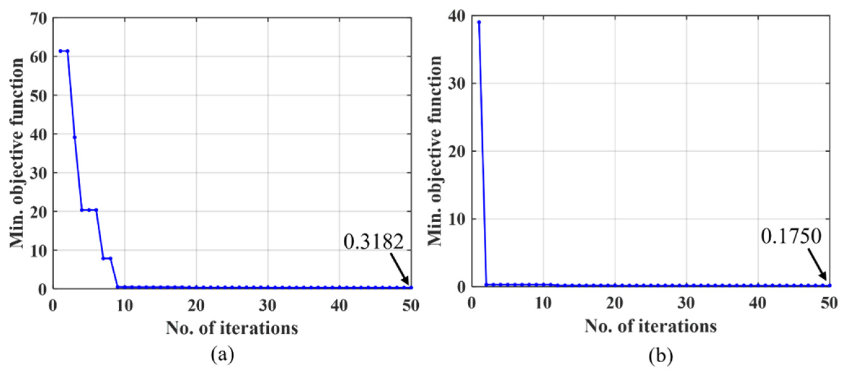
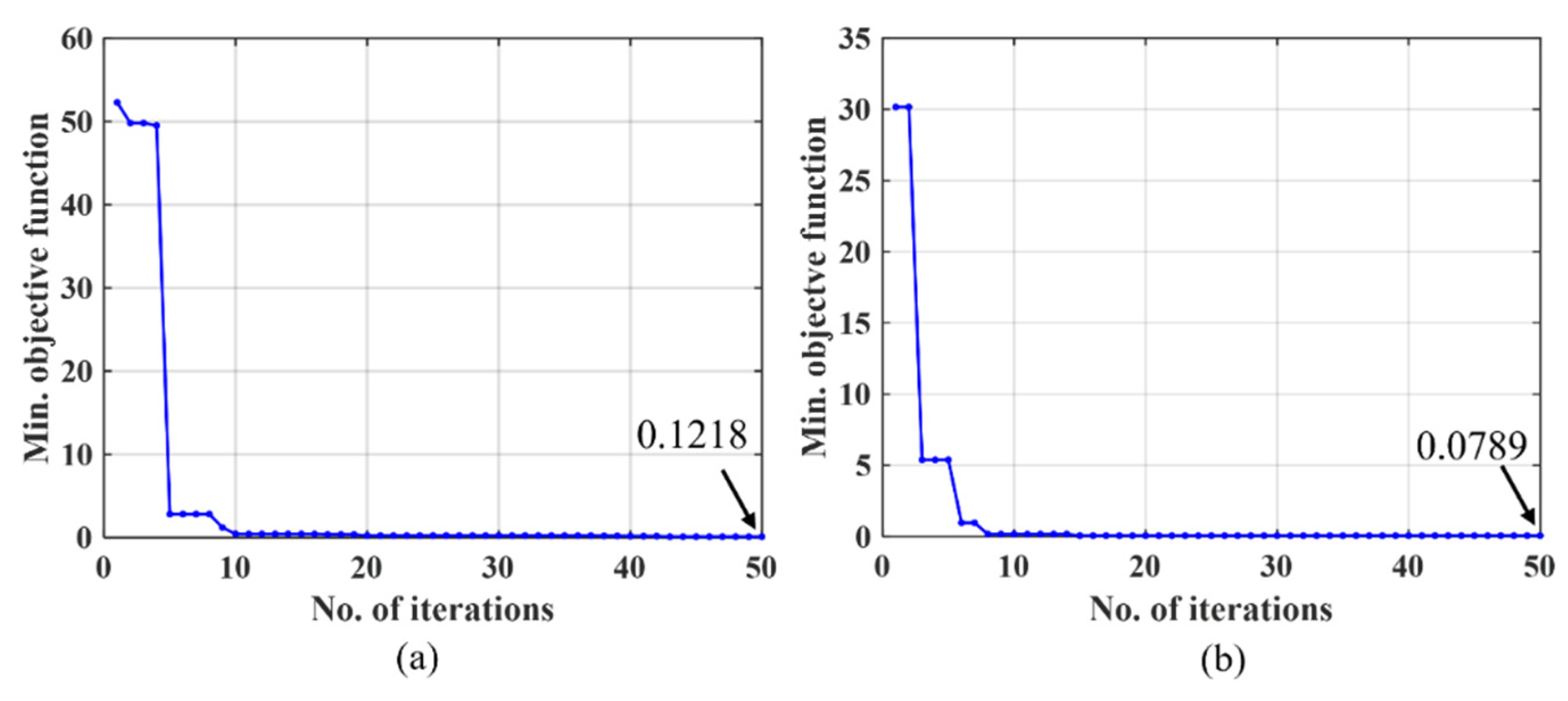
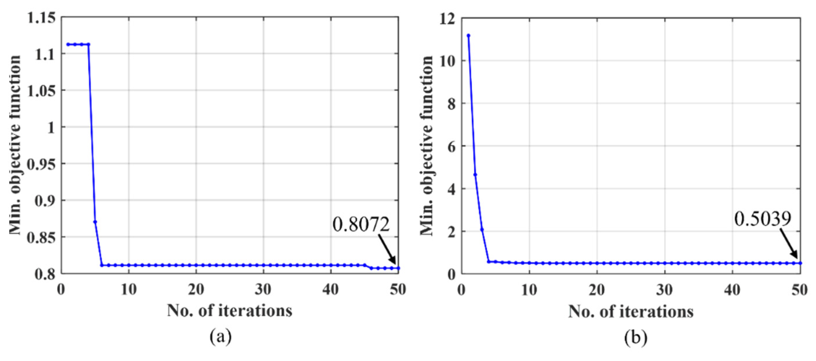
In contrast, the BO-RF model retained the same minimum leaf size and a nearly identical number of estimators, with a slightly deeper tree structure under the Qc condition, suggesting a stable learning process with moderate complexity adjustment to accommodate the different loading conditions. Moreover, the identified optimal parameters, namely, the regularization constant in the BO-SVR model, and the maximum tree depth and minimum leaf size in the BO-RF and BO-LSBoost models are crucial for mitigating the underfitting or overfitting while enhancing the generalizability performance of the models. Notably, the justification lies in the fact that excessively small or large values of the aforementioned parameters for a specific modeling problem can result in underfitting or overfitting [34,35,43], a challenge addressed in this study by carefully defining their search space to identify the optimal parameter. Herein, the tuning search space for maximum tree depth and minimum leaf size was determined based on the size of the training dataset utilized during BO. Additionally, the convergence curves of the average RMSE as objective function for BO are illustrated in Figure 17, Figure 18 and Figure 19, showing the well-stabilized convergence with no significant improvement observed beyond the employed 50 iterations. As a result, this confirms the efficiency and robustness of the BO in identifying the optimal hyperparameters of the adopted ML approaches.

5.3. Performance Evaluation of BO-SVR, BO-RF, and BO-LSBoost Models

To evaluate the performance of the BO-SVR, BO-RF, and BO-LSBoost models, each adopted ML approach was retrained with its respective optimal parameters on the aggregated training dataset. These trained models were aimed to evaluate the generalizability and prediction accuracy on the completely unseen testing dataset, as shown in Figure 16, using the assessment metrics. Herein, four commonly adopted assessment metrics for regression problems were employed: RMSE, mean absolute error (MAE), Akaike information criterion (AIC), and the coefficient of determination (R2), as defined in Equations (12)–(15). Specifically, the RMSE and MAE reflect the overall error distribution as model precision and accuracy, respectively; AIC represent the model robustness by considering the number of input variables while penalizing the most complex model; and R2 measures the good of fit between the actual and predicted target variables.
R M S E = 1 n i = 1 n y i y i ^ 2
M A E = 1 n i = 1 n y i y i ^
A I C = 1 n i = 1 n y i y i ^ 2 e 2 k n
R 2 = 1 i = 1 n y i y i ^ 2 i = 1 n y i y ¯ 2
where n represents the number of samples, k represents the number of input variables, and y i , y i ^ , and y ¯ represents the actual, predicted, and mean values, respectively.
Table 4 and Table 5 summarize the assessment metrics computed on the training and testing datasets for the BO-SVR, BO-RF, and BO-LSBoost models predicting the LTB capacity under one-point (central) and two-point loading conditions. Notably, the prediction performance was evaluated using ML models trained with their Bayesian-optimized parameters, thereby assisting in overcoming the overfitting or underfitting and improving generalizability. This is evident from the overall close agreement between the training and testing dataset errors (RMSE, MAE, and AIC) in Table 4 and Table 5, with neither excessive train–test discrepancy (overfitting) nor consistently high train–test errors (underfitting) under both loading conditions. Furthermore, as illustrated in Table 4 and Table 5, among the optimized ML models, BO-SVR consistently provided the most accurate, robust, and precise predictions across both loading cases, as indicated by their lower RMSE, MAE, and AIC values. In contrast, BO-LSBoost achieved competitive prediction accuracy but with modestly higher RMSE, MAE, and AIC values than BO-SVR, whereas BO-RF exhibited the greatest errors and the widest train–test differences under both loading scenarios. Specifically, as shown in Table 4 and Table 5, all optimized models showed lower average error metrics for predicting the LTB resistance under two-point than under one-point (central) loading: average RMSE, MAE, and AIC decreased by 35.40%, 36.95%, and 35.34% for BO-SVR; 38.44%, 37.71%, and 38.45% for BO-RF; and 58.33%, 61.10%, and 58.27% for BO-LSBoost, respectively. These improvements indicate that the optimized ML models adapt and generalize well to the underlying response complexity of two-point loading, with the greatest relative accuracy gains for BO-LSBoost and the consistently best absolute accuracy for BO-SVR. Moreover, the average R2 values were approximately equal to unity across both loading cases, indicating strong goodness of fit between the key influencing parameters and the LTB capacity of PS steel beams.
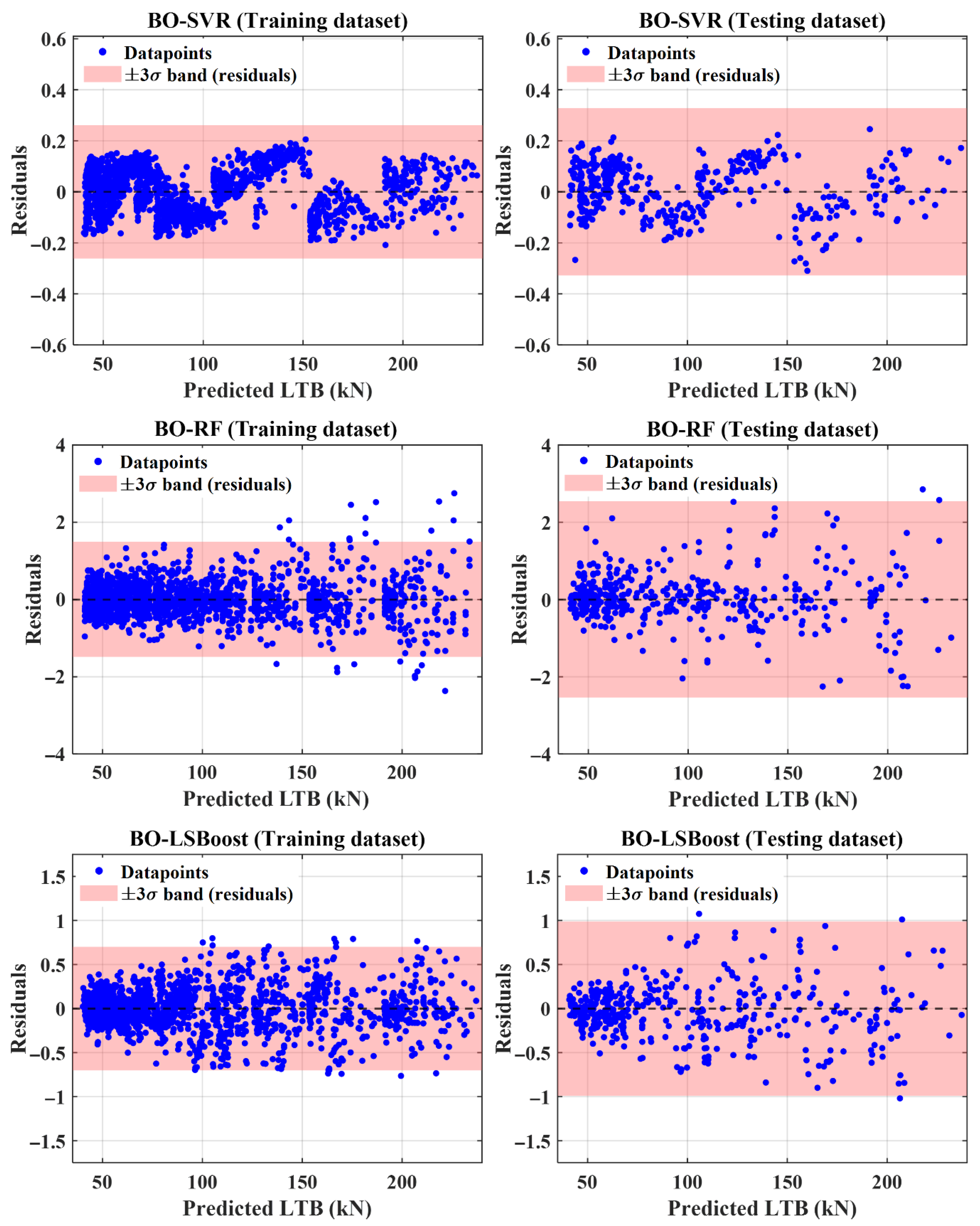
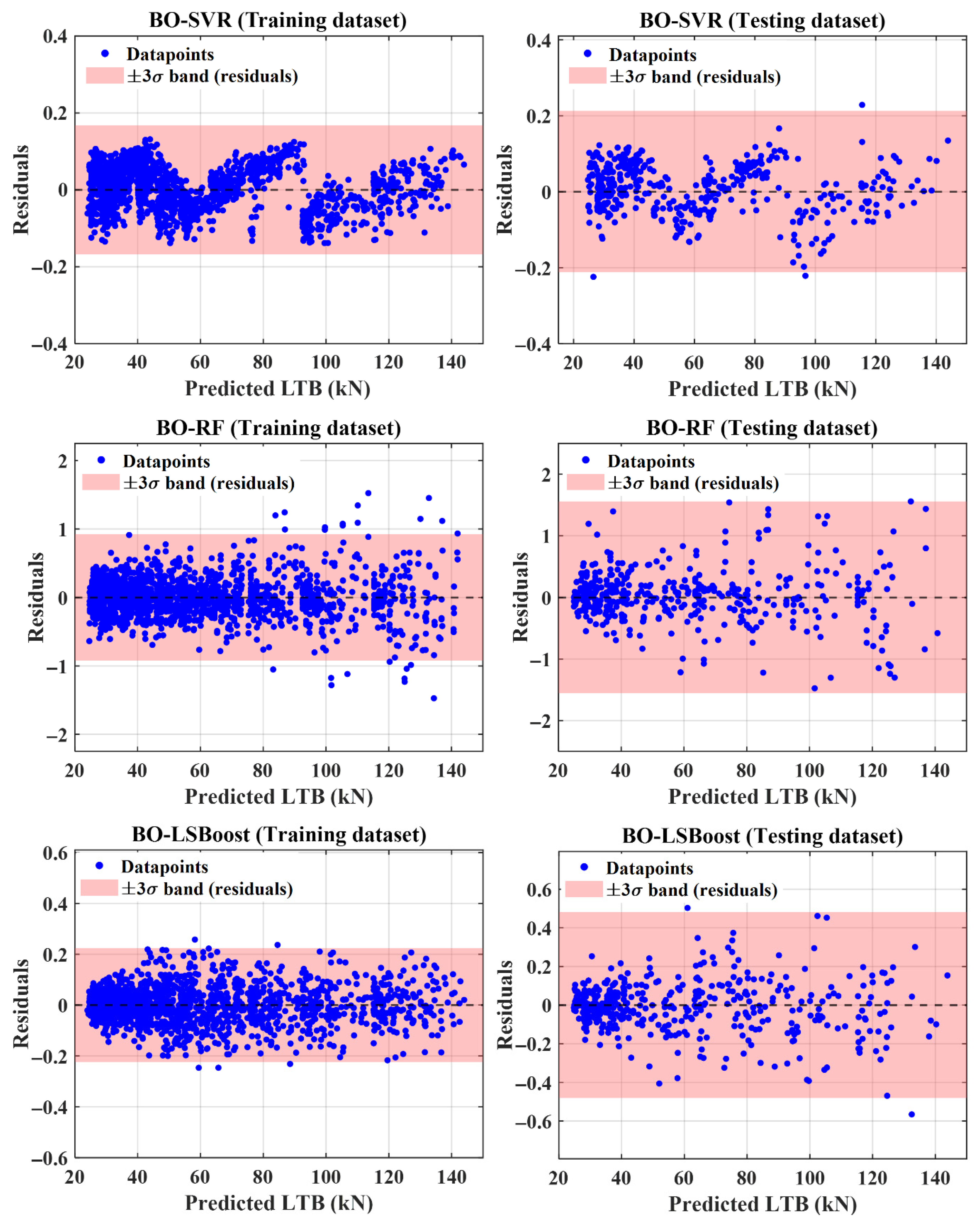
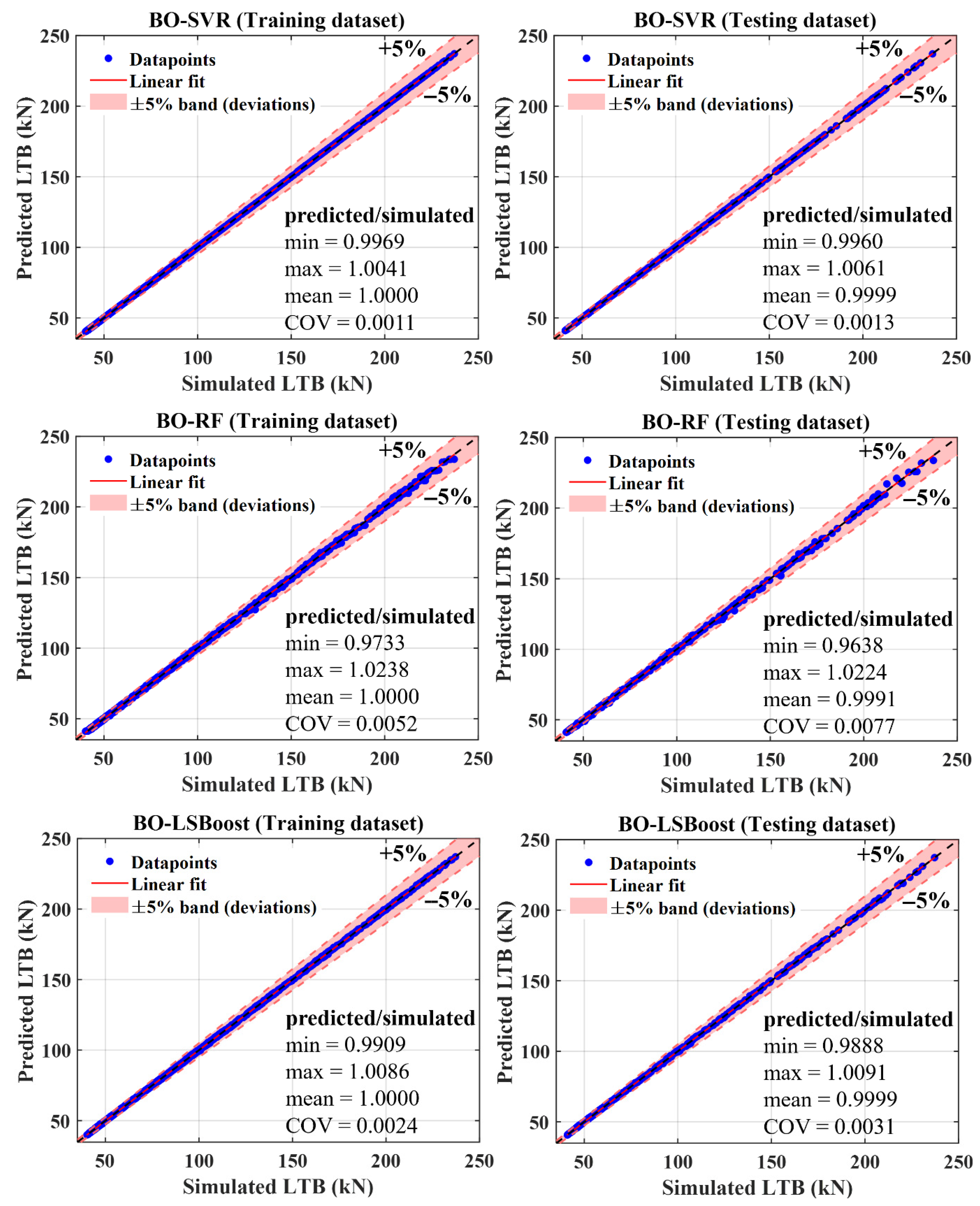
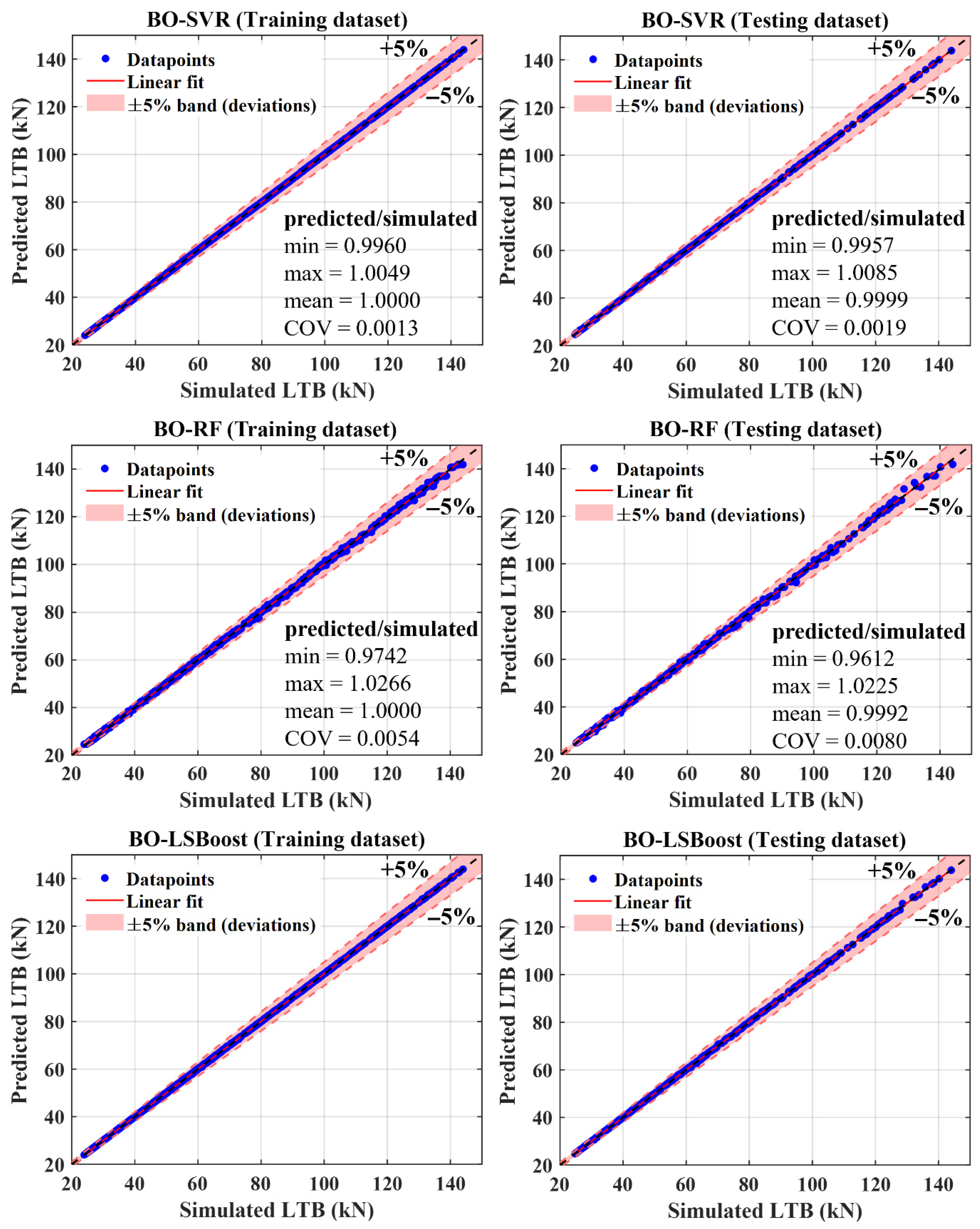
As an aspect of the result visualization, Figure 20 and Figure 21 illustrate the residual plots for the training and testing datasets under one-point (central) and two-point loading conditions. Residuals, defined as the difference between the simulated (FEM) and predicted LTB capacity, were centered around the zero line and were randomly dispersed without any obvious trend in variance across the prediction range. Notably, the vast majority of the datapoints lied within the ±3σ residual band with comparable train–test patterns, thereby indicating good generalization and well-fitted BO-ML models. Specifically, across both loading conditions, BO-SVR showed the tightest and symmetrical spread; BO-LSBoost exhibited a slightly broader yet largely pattern-free scatter and remained competitive with BO-SVR; and BO-RF demonstrated the widest spread with a few isolated outliers and mild increase in variance at mid-to-high predicted values. Overall, the residual spreads were marginally smaller under two-point loadings, consistent with the lower average errors and the comparative predictive performance, as reported in Table 4 and Table 5. Additionally, the regression analysis plots in Figure 22 and Figure 23 displayed symmetrical clustering of the datapoints around the 1:1 bisector line (45° black dashed line), with the fitted linear trend coinciding with the 45° bisector and majority of the datapoints lying within ±5% deviation band. This further confirms the better generalizability of the Bayesian-optimized ML models with negligible bias, strong goodness of fit, and high predictive accuracy for LTB capacity under both loading cases.
Table 6 compares the computational costs among the Bayesian-optimized ML models. As shown in Table 6, the BO stage dominated the overall runtime, whereas retraining the ML models with the acquired optimal parameters required only few seconds. Furthermore, under both loading cases, BO-SVR was computationally the most expensive, whereas the BO-LSBoost was the most efficient. Consequently, BO-LSBoost, given its comparative predictive performance and generalizability at lower computational cost than BO-SVR, can be adopted for accurate, precise, and robust predictions of LTB capacity under one-point (central) and two-point loadings in diverse practical applications.

5.4. Interpretability (Feature Importance) Analysis

ML approaches are often perceived as “black boxes” by structural engineers because their predictions can be difficult to explain and interpret. To overcome this limitation, several explainable ML techniques are available, which provide global (model-level) and local (instance-level) insights into trained ML models [60]. These techniques quantify and visualize how input parameters influence predictions and help assess whether the learned relationships are consistent with the established structural behavior knowledge. This section presents the interpretability analysis of the Bayesian-optimized ML models using permutation- and SHapley Additive exPlanations (SHAP)-based relative (global) feature importance methods.
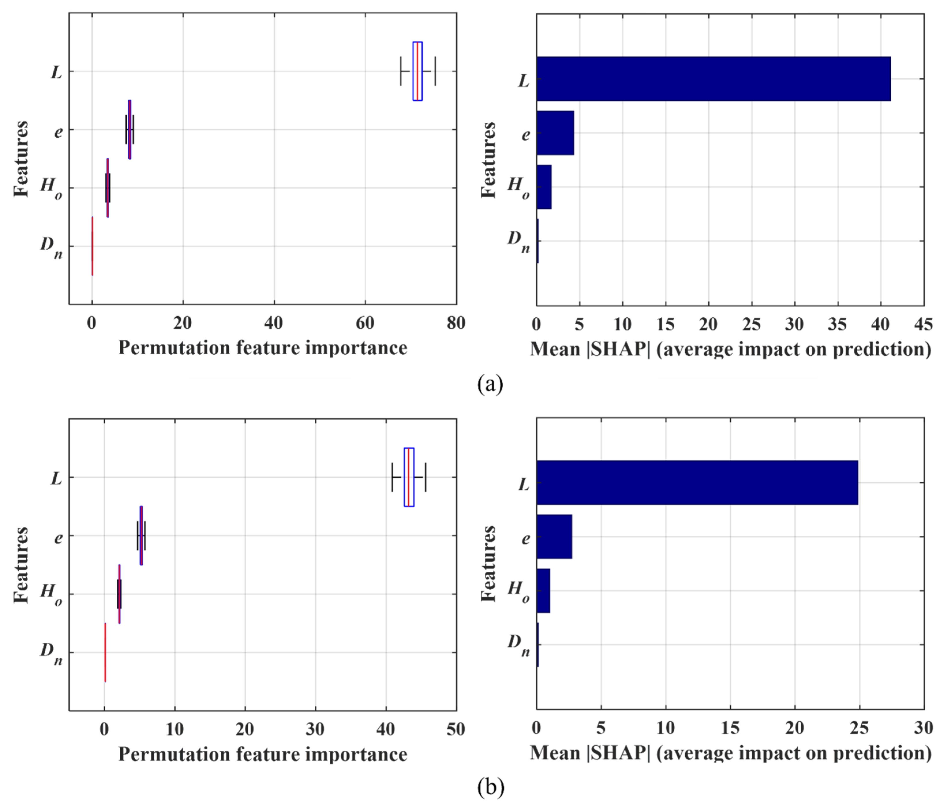
The permutation feature importance quantifies the decrease in model performance when the features values are randomly shuffled. A feature with a more significant decrease in performance is more important than other features. In this study, performance was evaluated using RMSE to ensure precision, and each feature was shuffled multiple times to estimate the mean and standard deviation of its importance score. In contrast, the SHAP method [61] explains the model predictions by assigning each feature a Shapley value determined using the coalition game theory [62]. Shapely values represents the average marginal contribution to the predictions, computed over all possible subsets (coalitions) of features with expectations taken over a background data distribution. SHAP adopts an additive feature attribution method, and the relative (global) feature importance is obtained using absolute average Shapley value across samples. Features with larger Shapley values are more important than others. Notably, the relative feature importance plots using permutation- and SHAP-based methods were similar for the optimized ML models under both considered loading conditions. Accordingly, because the BO-LSBoost models achieved comparatively accurate predictive performance and generalizability at lower computational cost than BO-SVR across both loading cases (as discussed in Section 5.3), we focus the subsequent discussion on their relative feature importance results.
Figure 24 illustrates the permutation- and SHAP-based relative feature importance plots for LTB capacity predictions under one (central)- and two-point loading conditions. Across both loading cases, the unbraced span length, L, over the entire dataset was identified as the dominant feature, significantly influencing the LTB predictions in both methods. This observation is consistent with the governing role of geometric slenderness in global buckling behavior. Subsequently, the eccentricity, e, and pre-stressing force, Ho, exhibited secondary but significant effects, whereas the number of deviators, Dn, contributed negligibly in predicting the LTB capacity in either loading case according to both methods. Notably, when the span length is fixed, the relative importance of e and Ho increases, highlighting the dominant role of pre-stressing parameters influencing the LTB resistance for a given span length. Moreover, the magnitude of SHAP-based feature attributions demonstrated that L, e, and Ho impacted LTB behavior more significantly under one-point (central) than under two-point loadings.
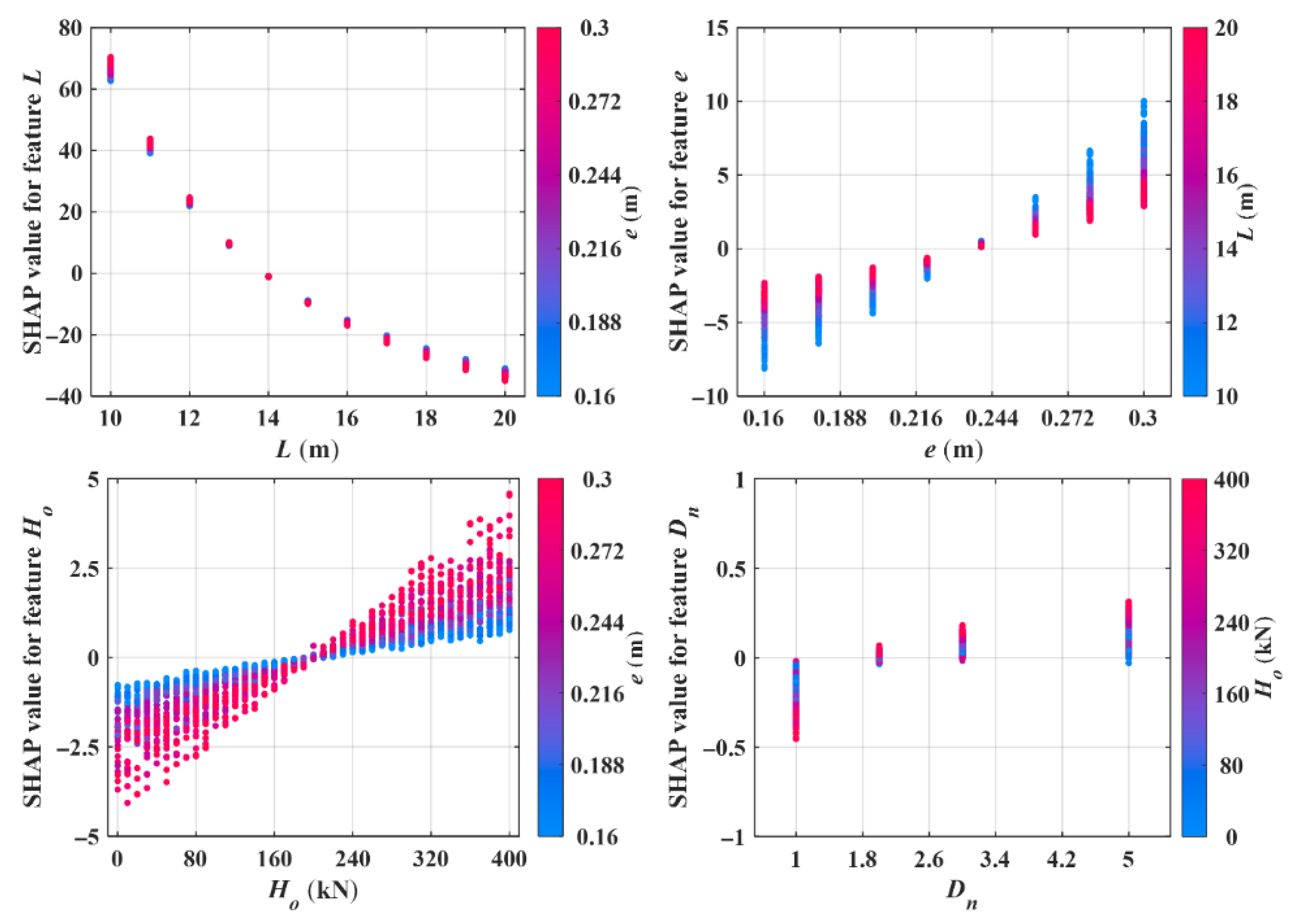
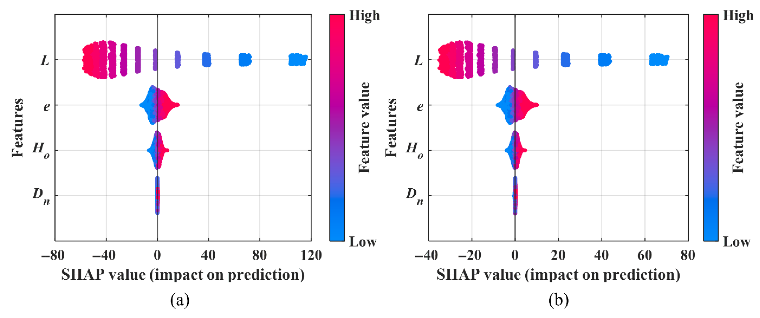
Beyond relative feature importance, the SHAP summary (beeswarm) plots shown in Figure 25 were analyzed for the BO-LSBoost models to provide local (instance-level) insights by combining feature values with feature effects. In these plots, each point represents a sample’s Shapley value for the feature: positive values indicate a positive effect in predicting LTB capacity, while negative values suggest a negative impact. The magnitude of the Shapley value reflects the strength of the effect on LTB capacity predictions, and the color encodes the feature value from low (blue) to high (red). Notably, as illustrated in Figure 25, the feature ordering (L, e, Ho, and Dn) was consistent across both loading scenarios and matched the global importance ranking shown in Figure 24. Furthermore, the beeswarm summary plots demonstrated that moderate-to-larger L values are predominately associated with negative Shapley values, i.e., increasing L reduces the predicted LTB capacity and vice versa for shorter spans. In contrast, higher values of e and Ho are mainly associated with positive SHAP values, implying an increased impact on the predicted LTB capacity as e and Ho increase. However, Dn remained tightly clustered around zero, indicating a negligible effect. These feature importance results aligned with the prior findings [21,39] and with the parametric studies and feature engineering analysis in Section 3.3 and Section 5.1, respectively, thereby confirming the effectiveness of the BO-LSBoost models in capturing the underlying mechanics of the PS structural systems under practical loading cases.
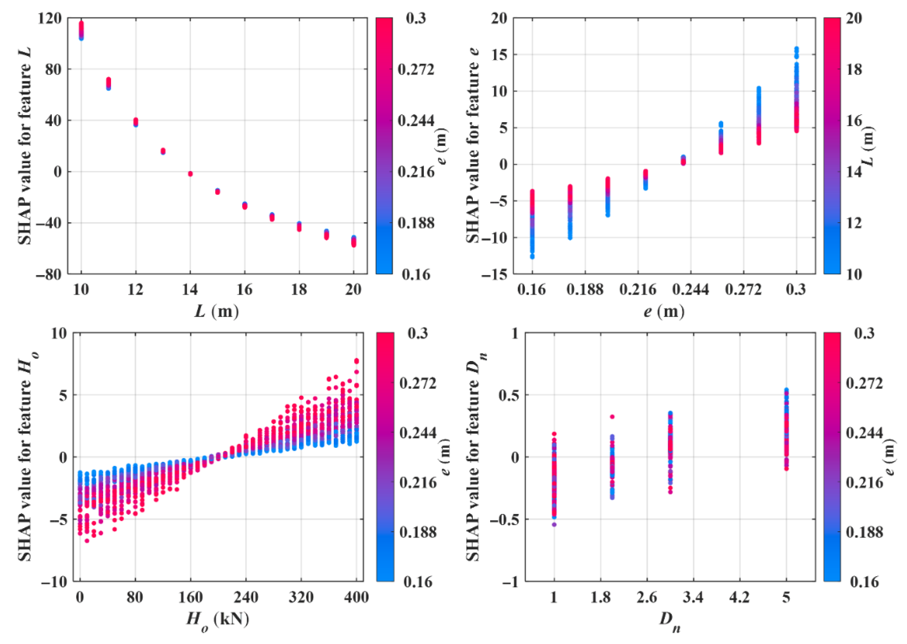
Figure 26 and Figure 27 illustrate the SHAP dependence plots, which represent the exact relationship between the BO-LSBoost predictions and the adopted critical features. In these plots, the feature’s (primary) sample values are shown on the x-axis, while the y-axis shows the corresponding SHAP values, i.e., the change in the predicted LTB capacity attributable to the primary feature for each sample. Moreover, the point color in Figure 20 and Figure 21 encodes a secondary feature that exhibited the strongest interaction with the considered primary (x-axis) feature. Interaction was defined by maximizing ( ρ s Z , ϕ X X ) over all candidate secondary features, Z , where ρ s is the partial Spearman rank correlation between Z and SHAP values, ϕ X , of the primary feature X , computed conditionally on X to mitigate collinearity and better capture interaction-driven variations in ϕ X . As illustrated in Figure 26 and Figure 27, L and Ho exhibited the strongest interaction with e, whereas e demonstrated strongest interaction with L across both loading cases. Specifically, an increase in L resulted in an exponential decrease in predicted LTB capacity, which was more significant for the PS beams with higher e. Conversely, increasing e increased the predicted LTB capacity, and the effect interacted with L being stronger for longer spans (slenderness-dominated) at low-to-moderate e but stronger for shorter spans at high e. Furthermore, as Ho increased, the predicted LTB capacity transitioned from a decrease at lower Ho to an increase at higher Ho, and the magnitude of this transition was amplified with e (stabilizing pre-bending moment, M p =   H o e ). Finally, under both loading scenarios, Dn showed a weak monotonic increase in predicted LTB capacity, with magnitudes that remained tightly clustered around zero and were largely insensitive to interactions with the secondary features e and Ho under one-point (central) and two-point loadings, respectively. These SHAP dependence results, while mostly consistent across both loading conditions and aligned with parametric studies in Section 3.3, effectively supported the interpretability of the BO-LSBoost models in capturing the complex, inherent behavior of the PS structural systems to reliably predict the LTB capacity.

6. Conclusions

This study proposed an integrated numerical, experimental, and ML framework for predicting the LTB capacity of un-bonded PS thin-walled steel I-beams subjected to non-uniform bending induced by one-point (central) and two-point vertical loadings. Specifically, despite extensive prior research, the exact analytical solutions of these systems are either not available or can be extremely complicated, as the resulting governing differential equations contain variable coefficients particularly under non-uniform bending and pre-stressing interactions. To address this limitation, a numerical investigation was first conducted by developing FE models in ABAQUS, incorporating the key influencing variables, including unbraced span length, tendon eccentricity, deviator configuration, and pre-stressing force. These FE models were then strategically validated through a two-step process against the approximate analytical solution and experimental results, enabling their reliability for use in a broad parametric study to generate a comprehensive dataset covering a wide range of practical PS beam configurations and loading conditions. Subsequently, Bayesian-optimized ML approaches, BO-SVR, BO-RF, and BO-LSBoost, were developed using the generated dataset to predict the LTB capacity under one-point (central) and two-point loading conditions. The implementation of these data-driven methods, in comparison to numerical model-based FE methods, significantly reduced the computational burden in simulating complex structural behavior while incorporating interaction effects of critical geometric and pre-stressing parameters. The main conclusions can be drawn as follows:
  • An approximate analytical solution using the Rayleigh–Ritz method for one-point loading was presented, while two- and five-term numerical solutions were presented in Table 2.
  • FE models for PS system under non-uniform bending from (central) one- and two-point vertical loadings were developed, which were in good agreement with five-term analytical solutions by the Ritz method and the experimental results, demonstrating that the FE approach can reliably reproduce the observed LTB behavior and ultimate capacity.
  • The adopted ML models trained with Bayesian-optimized parameters effectively addressed the overfitting or underfitting with improved generalizability based upon the close agreement between the training and testing dataset errors.
  • The LTB capacity predicted by the BO-ML models demonstrated negligible bias and strong goodness of fit (R2  1 ) with the simulated numerical data. Among the adopted BO-ML models, BO-SVR consistently achieved the best absolute accuracy (lowest RMSE, MAE, and AIC) across both loading cases, BO-LSBoost was competitive with the largest relative accuracy gains for two-point loading, and BO-RF showed the highest errors.
  • Among the developed BO-ML models, BO-LSBoost, due to its comparative predictive accuracy, strong generalizability, and computational efficiency over BO-SVR, can be employed to reliably and robustly predict the LTB capacity, particularly under practical loading conditions where conventional analytical approaches are infeasible.
  • Building upon the detailed interpretability analysis of the BO-ML models at a fixed unbraced span length, tendon eccentricity, e, and initial pre-stressing force, Ho, were identified as the dominant pre-stressing parameters influencing the prediction of LTB capacity, while the effect of the number of deviators, Dn, was found to be negligible. Moreover, the SHAP dependence analysis indicated that increases in e and Ho are associated with predominantly positive contributions to the predicted LTB capacity, reflecting their stabilizing interaction effects within the pre-stressed system. The interpretability results demonstrate that the BO-ML models are capable of effectively capturing the complex and physically meaningful influence of pre-stressing parameters on the inherent LTB behavior of PS steel structural systems from the training dataset. In practice, these insights can support informed engineering decision-making by allowing designers to prioritize influential parameters and thus improving structural design efficiency by reducing unnecessary conservatism.
Apparently, further studies may extend the proposed ML framework to include additional failure modes such as local global interaction and web distortion, enabling unified prediction across multiple buckling mechanisms.

Author Contributions

Conceptualization, A.T.A., M.-Y.K. and A.I.M.; methodology, A.T.A., M.-Y.K. and A.I.M.; software, A.T.A. and A.I.M.; validation, A.T.A. and A.I.M.; formal analysis, A.T.A. and A.I.M.; investigation, A.T.A. and A.I.M.; resources, A.T.A. and A.I.M.; data curation, A.T.A. and A.I.M.; writing—original draft preparation, A.T.A. and A.I.M.; writing—review and editing, A.T.A., M.-Y.K., I.U.K. and A.I.M.; visualization, A.T.A., I.U.K. and A.I.M.; supervision, A.I.M.; project administration, M.-Y.K. and A.I.M.; funding acquisition, M.-Y.K. All authors have read and agreed to the published version of the manuscript.

Funding

This work was supported by the National Research Foundation of Korea, which is funded by the Korean government grant number [NRF-2021R1A2C1009716].

Data Availability Statement

The data are available on request from the corresponding author.

Conflicts of Interest

Author Agha Intizar Mehdi is employed by the ENVICO Co., Ltd. The remaining authors declare that the research was conducted in the absence of any commercial or financial relationships that could be construed as a potential conflict of interest.

Abbreviations

The following abbreviations are used in this manuscript:
LTBlateral torsional buckling
PSpre-stressed
FEfinite element
MLmachine learning
SVRsupport vector regression
RFrandom forest
LSBoostleast-square boosting
BOBayesian optimization
BO-MLBayesian-optimized machine learning
BO-SVRBayesian-optimized support vector regression
BO-RFBayesian-optimized random forest
BO-LSBoostBayesian-optimized least-square boosting
SHAPSHapley Additive exPlanations

Appendix A

A steel I-section beam externally post-tensioned using straight tendon cables with a constant eccentricity, e , anchored through rigid deviators (see Figure A1), is considered. The structural response is evaluated in two distinct loading stages.
During the first stage, an initial prestressing force, H o , is applied to the tendon. This pre-stressing force induces a uniform axial stress across the beam section together with a bending stress caused by the eccentricity, e .
In the second stage, an externally applied bending moment produces downward deflection of the pre-stressed beam. This deformation results in an increase in tendon force, which is partially transferred back to the steel member. Consequently, an additional uniform bending moment is generated in the beam. According to Kim et al. [23], the total tendon force, H , and the corresponding internal axial force, F 1 , and bending moment, M 3 , in the beam can be expressed as:
H = H o + C M M ,   F 1 = H ,   M 3 = M H e C M = e E A c + H o E I 3 + E A c e 2 + I 3 / A
where A c denotes the tendon cross-sectional area.
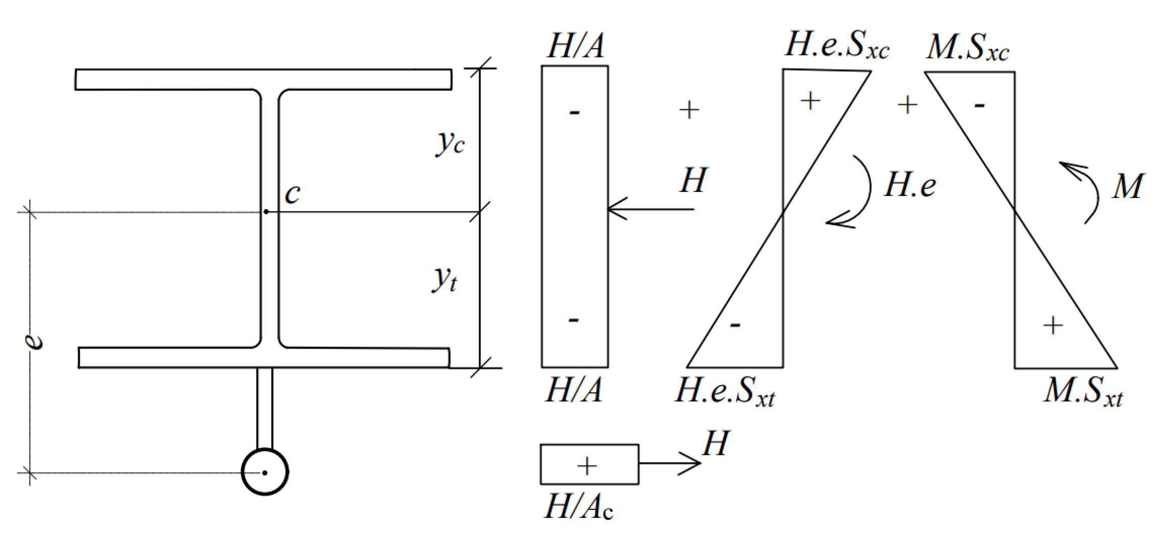
Figure A1. Stress distributions of the PS beam.
Buildings 16 01153 g0a1
Figure A1 illustrates the stress distribution within the pre-stressed beam section due to the initial tendon force, H o , and the applied bending moment, M . The combined effect of these actions produces resultant stresses at the top and bottom flanges, as well as in the tendon. As the external moment increases, three potential yielding conditions may occur in the pre-stressed section: yielding of the compression flange, yielding of the tension flange, and yielding of the tendon cable. Denoting F y and F y c as the yield stresses of the steel beam and tendon, respectively, the corresponding critical yielding moments can be determined as:
Compression   flange   yielding :   F y = H o + C M M y c e M y c S x c H o + C M M y c A Tension   flange   yielding :     F y = M y t H o + C M M y t e S x t H o + C M M y t A Tendon   cable   yielding :     F y c = H o + C M M y , c a b A c
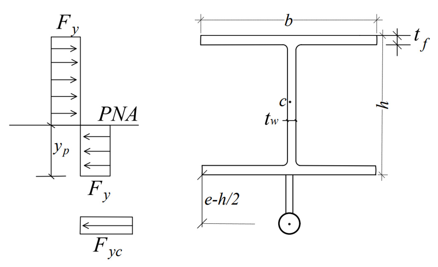
where M y t and M y c represent the bending moments causing yielding at the top and bottom flanges of the pre-stressed beam, and M y , c a b corresponds to tendon yielding. The yield capacity of the pre-stressed beam is taken as the minimum of these three values. The plastic moment capacity, M p , is obtained by enforcing equilibrium between the compressive, tensile, and tendon force resultants, as shown in Figure A2.
Figure A2. A fully plastic PS beam section.
Buildings 16 01153 g0a2
Considering that the plastic neutral axis lies within the web, the neutral axis position is first determined by solving Equation (A3). Subsequently, the plastic moment capacity of the pre-stressed section can be calculated from Equation (A4):
F y b t f + h t f y p t w t w y p t f b t f = F y c A c
M P = F y b t f h t f / 2 y p + h t f y p t w h t f y p / 2 + t w y p t f y p t f / 2 + b t f y p t f / 2 + F y c A c e h / 2 + y p

References

  1. Troitsky, M. Prestressed Steel Bridges: Theory and Design; Kluwer Academic Publishers: Alphen aan den Rijn, The Netherlands, 1990. [Google Scholar]
  2. Park, S.; Kim, T.; Kim, K.; Hong, S.-N. Flexural behavior of steel I-beam prestressed with externally unbonded tendons. J. Constr. Steel Res. 2010, 66, 125–132. [Google Scholar] [CrossRef] [Scilit]
  3. Ren, Y.; Wang, Y.; Wang, B.; Ban, H.; Song, J.; Su, G. Flexural behavior of steel deep beams prestressed with externally unbonded straight multi-tendons. Thin-Walled Struct. 2018, 131, 519–530. [Google Scholar] [CrossRef] [Scilit]
  4. Kim, M.-Y.; Hayat, U.; Kim, S.-B.; Mehdi, A.I. Stabilizing effects of discrete deviators on LTB of mono-symmetric thin-walled beams pre-stressed by rectilinear tendon cables. Thin-Walled Struct. 2022, 176, 109329. [Google Scholar] [CrossRef] [Scilit]
  5. Belenya, E. Prestressed Load-Bearing Metal Structures; Mir Publishers: Moscow, Russia, 1977. [Google Scholar]
  6. Wadee, M.A.; Hadjipantelis, N.; Bazzano, J.B.; Gardner, L.; Lozano-Galant, J.A. Stability of steel struts with externally anchored prestressed cables. J. Constr. Steel Res. 2020, 164, 105790. [Google Scholar] [CrossRef] [Scilit]
  7. Gosaye, J.; Gardner, L.; Wadee, M.A.; Ellen, M.E. Compressive behaviour and design of prestressed steel elements. Structures 2016, 5, 76–87. [Google Scholar] [CrossRef] [Scilit]
  8. Hadjipantelis, N.; Gardner, L.; Wadee, M.A. Prestressed cold-formed steel beams: Concept and mechanical behaviour. Eng. Struct. 2018, 172, 1057–1072. [Google Scholar] [CrossRef] [Scilit]
  9. De Araujo, R.; De Andrade, S.; Vellasco, P.d.S.; Da Silva, J.; De Lima, L. Experimental and numerical assessment of stayed steel columns. J. Constr. Steel Res. 2008, 64, 1020–1029. [Google Scholar] [CrossRef] [Scilit]
  10. Wu, K.; Wadee, M.A.; Gardner, L. Interactive buckling in prestressed stayed beam-columns. Int. J. Mech. Sci. 2020, 174, 105479. [Google Scholar] [CrossRef] [Scilit]
  11. Wu, K.; Wadee, M.A.; Gardner, L. Prestressed stayed beam-columns: Sensitivity to prestressing levels, pre-cambering and imperfections. Eng. Struct. 2021, 226, 111344. [Google Scholar] [CrossRef] [Scilit]
  12. Belletti, B.; Gasperi, A. Behavior of prestressed steel beams. J. Struct. Eng. 2010, 136, 1131–1139. [Google Scholar] [CrossRef] [Scilit]
  13. Ghafoori, E.; Motavalli, M. Lateral-torsional buckling of steel I-beams retrofitted by bonded and un-bonded CFRP laminates with different pre-stress levels: Experimental and numerical study. Constr. Build. Mater. 2015, 76, 194–206. [Google Scholar] [CrossRef] [Scilit]
  14. Kambal, M.E.M.; Jia, Y. Theoretical and experimental study on flexural behavior of prestressed steel plate girders. J. Constr. Steel Res. 2018, 142, 5–16. [Google Scholar] [CrossRef] [Scilit]
  15. Chen, Z.; Wu, Y.; Yin, Y.; Shan, C. Formulation and application of multi-node sliding cable element for the analysis of Suspen-Dome structures. Finite Elem. Anal. Des. 2010, 46, 743–750. [Google Scholar] [CrossRef] [Scilit]
  16. Hathout, I.A.-S. Stability Analysis of Space Stayed Columns by the Finite Element Method. Master’s Thesis, University of Windsor, Windsor, ON, Canada, 1977. [Google Scholar]
  17. Khosla, C. Buckling Loads of Stayed Columns Using the Finite Element Method. Master’s Thesis, University of Windsor, Windsor, ON, Canada, 1975. [Google Scholar]
  18. Zhou, B.; Accorsi, M.; Leonard, J. Finite element formulation for modeling sliding cable elements. Comput. Struct. 2004, 82, 271–280. [Google Scholar] [CrossRef] [Scilit]
  19. Kim, M.-Y.; Nanzad, N.; Hayat, U. Effects of un-bonded deviators on the out-of-plane buckling of steel H-beams pre-stressed by a straight tendon cable. Eng. Struct. 2020, 214, 110566. [Google Scholar] [CrossRef] [Scilit]
  20. Zhang, W.-F. Symmetric and antisymmetric lateral–torsional buckling of prestressed steel I-beams. Thin-Walled Struct. 2018, 122, 463–479. [Google Scholar] [CrossRef] [Scilit]
  21. Kim, M.-Y.; Hayat, U.; Mehdi, A.I. Lateral–torsional buckling of steel beams pre-stressed by straight tendons with a single deviator. Thin-Walled Struct. 2021, 163, 107642. [Google Scholar] [CrossRef] [Scilit]
  22. Kim, M.-Y.; Kim, N.-K.; Hayat, U. Flexural buckling and second-order analysis of pre-stressed steel beams with un-bonded/bonded deviators. Thin-Walled Struct. 2021, 164, 107806. [Google Scholar] [CrossRef] [Scilit]
  23. Kim, M.-Y.; Mehdi, A.I.; Hayat, U. Spatial stability of pre-stressed mono-symmetric steel beams with un-bonded/bonded deviators under compression and end moments. J. Constr. Steel Res. 2022, 189, 107078. [Google Scholar] [CrossRef] [Scilit]
  24. Kim, M.; Mehdi, A.; Kim, S. FE Analysis on In-Plane and Out-of-Plane Buckling of Steel Beams with Externally Prestressed Rectilinear Tendons. J. Korean Soc. Steel Constr. 2022, 34, 77–88. [Google Scholar] [CrossRef] [Scilit]
  25. Kim, S.-B.; Mehdi, A.I.; Kim, M.-Y. Experimental evaluation on LTB strength of steel beams externally pre-stressed with un-bonded tendon bar. Int. J. Steel Struct. 2024, 24, 488–505. [Google Scholar] [CrossRef] [Scilit]
  26. Sun, H.; Burton, H.V.; Huang, H. Machine learning applications for building structural design and performance assessment: State-of-the-art review. J. Build. Eng. 2021, 33, 101816. [Google Scholar] [CrossRef] [Scilit]
  27. Thai, H.-T. Machine learning for structural engineering: A state-of-the-art review. Structures 2022, 38, 448–491. [Google Scholar] [CrossRef] [Scilit]
  28. Rabi, R.R. Shear capacity assessment of hollow-core RC piers via machine learning. Structures 2025, 76, 108961. [Google Scholar] [CrossRef] [Scilit]
  29. Rabi, R.R.; Monti, G. Machine learning-derived equations for seismic fragility of hollow-core bridge piers using analytical models and visible parameters. Structures 2025, 75, 108792. [Google Scholar] [CrossRef] [Scilit]
  30. Rahmat Rabi, R.; Monti, G. Genetic Algorithm-Based Model Updating in a Real-Time Digital Twin for Steel Bridge Monitoring. Appl. Sci. 2025, 15, 4074. [Google Scholar] [CrossRef] [Scilit]
  31. Sharifi, Y.; Moghbeli, A.; Hosseinpour, M.; Sharifi, H. Neural networks for lateral torsional buckling strength assessment of cellular steel I-beams. Adv. Struct. Eng. 2019, 22, 2192–2202. [Google Scholar] [CrossRef] [Scilit]
  32. Ferreira, F.P.V.; Shamass, R.; Limbachiya, V.; Tsavdaridis, K.D.; Martins, C.H. Lateral–torsional buckling resistance prediction model for steel cellular beams generated by Artificial Neural Networks (ANN). Thin-Walled Struct. 2022, 170, 108592. [Google Scholar] [CrossRef] [Scilit]
  33. Wu, K.; Qiang, X.; Xing, Z.; Jiang, X. Buckling in prestressed stayed beam–columns and intelligent evaluation. Eng. Struct. 2022, 255, 113902. [Google Scholar] [CrossRef] [Scilit]
  34. Seghier, M.E.A.B.; Carvalho, H.; de Faria, C.C.; Correia, J.A.; Fakury, R.H. Numerical analysis and prediction of lateral-torsional buckling resistance of cellular steel beams using FEM and least square support vector machine optimized by metaheuristic algorithms. Alex. Eng. J. 2023, 67, 489–502. [Google Scholar] [CrossRef] [Scilit]
  35. Degtyarev, V.V.; Tsavdaridis, K.D. Buckling and ultimate load prediction models for perforated steel beams using machine learning algorithms. J. Build. Eng. 2022, 51, 104316. [Google Scholar] [CrossRef] [Scilit]
  36. de Oliveira, V.M.; de Carvalho, A.S.; Rossi, A.; Hosseinpour, M.; Sharifi, Y.; Martins, C.H. Data-driven design approach for the lateral-distortional buckling in steel-concrete composite cellular beams using machine learning models. Structures 2024, 61, 106018. [Google Scholar] [CrossRef] [Scilit]
  37. Hajdú, G.; Bektaş, N.; Müller, A. Machine learning models for the elastic-critical buckling moment of sinusoidal corrugated web beam. Results Eng. 2024, 23, 102371. [Google Scholar] [CrossRef] [Scilit]
  38. Kim, S.-B.; Kim, M.-Y. Improved formulation for spatial stability and free vibration of thin-walled tapered beams and space frames. Eng. Struct. 2000, 22, 446–458. [Google Scholar] [CrossRef] [Scilit]
  39. Mehdi, A.I.; Kim, M.-Y. LTB analysis of pre-stressed mono-symmetric thin-walled beams with deviators under non-uniform bending moments using a simplified FEM. Structures 2023, 47, 2331–2346. [Google Scholar] [CrossRef] [Scilit]
  40. Hibbitt, Karlsson & Sorensen Inc. ABAQUS User’s Manual; SIMULIA: Providence, RI, USA, 2019.
  41. Mehdi, A.I.; Zhang, F.; Kim, M.-Y. A spatial stability theory of thin-walled steel beams pre-stressed by spatially inclined un-bonded cables and its FE formulation. Thin-Walled Struct. 2024, 194, 111308. [Google Scholar] [CrossRef] [Scilit]
  42. Liu, J.-Z.; Li, S.; Guo, J.; Xue, S.; Chen, S.; Wang, L.; Zhou, Y.; Luo, T.X. Machine learning (ML) based models for predicting the ultimate bending moment resistance of high strength steel welded I-section beam under bending. Thin-Walled Struct. 2023, 191, 111051. [Google Scholar] [CrossRef] [Scilit]
  43. Ho, L.V.; Bui-Tien, T.; Wahab, M.A. A two-step failure identification approach using a stochastic optimization-based ensemble learning model for beams without pristine data. Eng. Struct. 2025, 334, 120253. [Google Scholar] [CrossRef] [Scilit]
  44. Nguyen, H.; Vu, T.; Vo, T.P.; Thai, H.-T. Efficient machine learning models for prediction of concrete strengths. Constr. Build. Mater. 2021, 266, 120950. [Google Scholar] [CrossRef] [Scilit]
  45. Shahriari, B.; Swersky, K.; Wang, Z.; Adams, R.P.; De Freitas, N. Taking the human out of the loop: A review of Bayesian optimization. Proc. IEEE 2015, 104, 148–175. [Google Scholar] [CrossRef] [Scilit]
  46. Wu, J.; Chen, X.-Y.; Zhang, H.; Xiong, L.-D.; Lei, H.; Deng, S.-H. Hyperparameter optimization for machine learning models based on Bayesian optimization. J. Electron. Sci. Technol. 2019, 17, 26–40. Available online: https://www.sciencedirect.com/science/article/pii/S1674862X19300047 (accessed on 1 December 2025).
  47. Asad, A.T.; Kim, B.; Cho, S.; Sim, S.-H. Prediction Model for Long-Term Bridge Bearing Displacement Using Artificial Neural Network and Bayesian Optimization. Struct. Control Health Monit. 2023, 2023, 6664981. [Google Scholar] [CrossRef] [Scilit]
  48. Vapnik, V. The Nature of Statistical Learning Theory; Springer Science & Business Media: Berlin/Heidelberg, Germany, 2013. [Google Scholar]
  49. Boser, B.E.; Guyon, I.M.; Vapnik, V.N. A training algorithm for optimal margin classifiers. In Proceedings of the Fifth Annual Workshop on Computational Learning Theory, Pittsburgh, PA, USA, 27–29 July 1992. [Google Scholar] [CrossRef] [Scilit]
  50. Chang, C.-C.; Lin, C.-J. Training v-support vector regression: Theory and algorithms. Neural Comput. 2002, 14, 1959–1977. [Google Scholar] [CrossRef] [Scilit]
  51. Kromanis, R.; Kripakaran, P. Support vector regression for anomaly detection from measurement histories. Adv. Eng. Inform. 2013, 27, 486–495. [Google Scholar] [CrossRef] [Scilit]
  52. Breiman, L.; Friedman, J.; Olshen, R.A.; Stone, C.J. Classification and Regression Trees; Chapman and Hall/CRC: Boca Raton, FL, USA, 2017. [Google Scholar]
  53. Leo, B. Random forests. Mach. Learn. 2001, 45, 5–23. [Google Scholar] [CrossRef] [Scilit]
  54. Friedman, J.H. Greedy function approximation: A gradient boosting machine. Ann. Stat. 2001, 29, 1189–1232. [Google Scholar] [CrossRef] [Scilit]
  55. Onat, O.; Tanyıldızı, H. Machine learning-based estimation of the out-of-plane displacement of brick infill exposed to earthquake shaking. Eng. Appl. Artif. Intell. 2024, 136, 109007. [Google Scholar] [CrossRef] [Scilit]
  56. Abbas, Q.; Ali, T.; Asad, A.T.; Aslam, M. Analyzing the impact of geosynthetic reinforcement on Sinkhole: A numerical investigation with Machine Learning approach. Eng. Fail. Anal. 2024, 157, 107915. [Google Scholar] [CrossRef] [Scilit]
  57. Akber, M.Z. Improving the experience of machine learning in compressive strength prediction of industrial concrete considering mixing proportions, engineered ratios and atmospheric features. Constr. Build. Mater. 2024, 444, 137884. [Google Scholar] [CrossRef] [Scilit]
  58. Xie, W.; Nie, W.; Saffari, P.; Robledo, L.F.; Descote, P.-Y.; Jian, W. Landslide hazard assessment based on Bayesian optimization–support vector machine in Nanping City, China. Nat. Hazards 2021, 109, 931–948. [Google Scholar] [CrossRef] [Scilit]
  59. Kohavi, R. A study of cross-validation and bootstrap for accuracy estimation and model selection. In Proceedings of the Fourteenth International Joint Conference on Artificial Intelligence, Montreal, QC, Canada, 20–25 August 1995. [Google Scholar]
  60. Naser, M. An engineer’s guide to eXplainable Artificial Intelligence and Interpretable Machine Learning: Navigating causality, forced goodness, and the false perception of inference. Autom. Constr. 2021, 129, 103821. [Google Scholar] [CrossRef] [Scilit]
  61. Lundberg, S.M.; Lee, S.-I. A unified approach to interpreting model predictions. In Advances in Neural Information Processing Systems; MIT Press: Cambridge, MA, USA, 2017; p. 30. [Google Scholar]
  62. Peleg, B. Introduction to the Theory of Cooperative Games; Springer: Berlin/Heidelberg, Germany, 1989; Volume 34. [Google Scholar]
Figure 1. A set of PS simple beams possessing straight tendon and two deviators. (a) An initial configuration with single tendons and two deviators prior to pre-stressing. (b) Deformed PS beam after initial pre-stressing. (c) PS beam with un-bonded deviators deformed under a central load, Qc.
Buildings 16 01153 g001
Figure 2. A PS simple beam with m-1 un-bonded deviators.
Buildings 16 01153 g002
Figure 3. FE modeling of a PS simple system. (a) FE model of a PS beam with two deviators under un-bonded tendon condition. (b) PS I-beam section.
Buildings 16 01153 g003
Figure 4. Deformed FE model of a PS simple beam after tendon pre-stressing (ABAQUS).
Buildings 16 01153 g004
Figure 5. FE model load cases for LTB of a PS simple beam with two deviators under un-bonded tendon conditions. (a) LTB of PS beam with un-bonded deviators under a central load, Qc. (b) LTB of PS beam with un-bonded deviators under two-point load, Qp (equally spaced at L / 3 ).
Buildings 16 01153 g005aBuildings 16 01153 g005b
Figure 6. Experimental set-up of steel beam externally pre-stressed with an un-bonded tendon used for the mechanism-level validation of the proposed FE modeling approach. (a) PS steel beam externally pre-stressed under two-point vertical loading. (b) Fixed anchorage. (c) Un-bonded mid-span deviator. (d) Pre-stressing anchorage. (e) Potentiometers and strain gages at mid-span.
Buildings 16 01153 g006
Figure 7. Force-displacement/strain diagram (Kim et al. [25]). (a) Lateral torsional buckled beam (front and side view). (b) Vertical displacement. (c) Lateral displacement. (d) Strain of top flange. (e) Strain of bottom flange.
Buildings 16 01153 g007
Figure 8. PS beam under a central load, Qc: (a) (e = 0.2 m, Dn = 5, Ho = 400 kN), (b) (L = 12 m, Dn = 5, Ho = 400 kN), (c) (L = 12 m, e = 0.2 m, Ho = 400 kN), and (d) (L = 12 m, e = 0.2 m, Dn = 5).
Buildings 16 01153 g008
Figure 9. PS beam under two-point loads, Qp: (a) (e = 0.2 m, Dn = 5, Ho = 400 kN), (b) (L = 12 m, Dn = 5, Ho = 400 kN), (c) (L = 12 m, e = 0.2 m, Ho = 400 kN), and (d) (L = 12 m, e = 0.2 m, Dn = 5).
Buildings 16 01153 g009
Figure 10. Schematic of the SVR mechanism.
Buildings 16 01153 g010
Figure 11. Schematic of the RF algorithm.
Buildings 16 01153 g011
Figure 12. Schematic of the LSBoost algorithm.
Buildings 16 01153 g012
Figure 13. Schematic of the Bayesian optimization with Gaussian process model.
Buildings 16 01153 g013
Figure 14. Range and distribution of the input parameters for ML modeling.
Buildings 16 01153 g014
Figure 15. Correlation matrix of the input parameters and target variables (Note: Qc and Qp represents the one (central)- and two-point loading conditions, respectively).
Buildings 16 01153 g015
Figure 16. The overall framework adopted for the parameter’s optimization of ML models via BO.
Buildings 16 01153 g016
Figure 17. Convergence of average RMSE as objective function for the BO-SVR models under: (a) one-point (central) loading, Qc, and (b) two-point loading, Qp.
Buildings 16 01153 g017
Figure 18. Convergence of average RMSE as objective function for the BO-RF models under: (a) one-point (central) loading, Qc, and (b) two-point loading, Qp.
Buildings 16 01153 g018
Figure 19. Convergence of average RMSE as objective function for the BO-LSBoost models under: (a) one-point (central) loading, Qc, and (b) two-point loading, Qp.
Buildings 16 01153 g019
Figure 20. Residual plots of the BO-ML models under one-point (central) loading, Qc.
Buildings 16 01153 g020
Figure 21. Residual plots of the BO-ML models under two-point loading, Qp.
Buildings 16 01153 g021
Figure 22. Regression analysis results of the BO-ML models under one-point (central) loading, Qc.
Buildings 16 01153 g022
Figure 23. Regression analysis results of the BO-ML models under two-point loading, Qp.
Buildings 16 01153 g023
Figure 24. Relative feature importance for the BO-LSBoost models under: (a) one-point (central) loading, Qc, and (b) two-point loading, Qp.
Buildings 16 01153 g024
Figure 25. SHAP beeswarm summary plots for the BO-LSBoost models: (a) one-point (central) loading, Qc, and (b) two-point loading, Qp.
Buildings 16 01153 g025
Figure 26. SHAP dependence plots for the BO-LSBoost in predicting LTB capacity under one-point (central) loading conditions, Qc.
Buildings 16 01153 g026
Figure 27. SHAP dependence plots for the BO-LSBoost in predicting LTB capacity under two-point loading conditions, Qp.
Buildings 16 01153 g027
Table 1. The material and geometric properties of bi-symmetric thin-walled cross sections.
PropertyBi-Symmetric Section
Elastic modulus, E206 GPa
Cross-sectional area of beam, A11,700 mm2
Cross-sectional area of tendon, Ac1257 mm2
Second moment of inertia with respect to y axis, I31.989 × 108 mm4
Second moment of inertia with respect to z axis, I26.750 × 107 mm4
Torsional constant of beam, J7.750 × 105 mm4
Warping moment of inertia with respect to x-axis, Iϕ1.371 × 106 mm6
Table 2. Comparison of LTB loads, Qc (kN), of PS beams with increase in deviators.
No. of DeviatorsRitz. SolutionFE Solution
One-Term (Equation (10))Two Terms
k   =   2
Five Terms
k   =   5
Dn = 1142.891st142.891st136.881st136.261st, 485.982nd
Dn = 3143.601st143.601st137.081st136.441st, 487.082nd
Dn = 5143.731st143.731st137.191st136.551st, 487.332nd
Dn = 7143.771st143.771st137.231st136.581st, 487.402nd
Table 3. Optimal hyperparameters for the SVR, RF, and LSBoost models.
BO-SVR
HyperparametersTuning Search SpaceLTB Under QcLTB Under Qp
Regularization constant[10−3, 103]984.2221986.5708
Gaussian kernel scale[10−3, 103]1.73601.6842
Error tube size[10−3, 102]0.0010.001
BO-RF
HyperparametersTuning Search SpaceLTB Under QcLTB Under Qp
No. of trees (estimators)[1, 512]500508
Maximum depth of trees[1, training size = 1760]965898
Minimum samples per leaf[1, training size/2 = 880]22
BO-LSBoost
HyperparametersTuning Search SpaceLTB Under QcLTB Under Qp
No. of boosting iterations[1, 512]505512
Maximum depth of trees[1, training size = 1760]514
Minimum samples per leaf[1, training size/2 = 880]12
Learning rate[0.001, 1]0.12380.1515
Table 4. Assessment metrics under one-point (central) loading condition.
BO-ML ModelsDatasetRMSEMAEAICR2
BO-SVRTraining0.08690.07490.08730.9999
Testing0.10960.08690.11160.9999
Average0.09830.08090.09950.9999
BO-RFTraining0.49480.34310.49710.9999
Testing0.84780.54150.86330.9998
Average0.67130.44230.68020.9999
BO-LSBoostTraining0.23390.17260.2350.9999
Testing0.33040.23650.33640.9999
Average0.28220.20460.28570.9999
Table 5. Assessment metrics under two-point loading condition.
BO-ML ModelsDatasetRMSEMAEAICR2
BO-SVRTraining0.0560.04680.05630.9999
Testing0.0710.05520.07230.9999
Average0.06350.05100.06430.9999
BO-RFTraining0.30690.21410.30830.9999
Testing0.51950.33690.5290.9998
Average0.41320.27550.41870.9999
BO-LSBoostTraining0.07450.05410.07490.9999
Testing0.16060.1050.16350.9999
Average0.11760.07960.11920.9999
Table 6. Computational cost comparison among the adopted BO-ML models.
BO-ML ModelsLTB Capacity Under One-Point (Central) Loading Condition, Qc
Optimization Time (s)Training Time
(s)
Total Computational Time (s/h)
BO-SVR1658.7215.381674.10/0.46
BO-RF773.192.42775.61/0.21
BO-LSBoost702.50.98703.48/0.19
BO-ML ModelsLTB Capacity Under Two-Point Loading Condition, Qp
Optimization Time (s)Training Time
(s)
Total Computational Time (s/h)
BO-SVR2148.7818.322167.10/0.60
BO-RF872.523.15875.67/0.24
BO-LSBoost819.311.35820.23/0.22
Disclaimer/Publisher’s Note: The statements, opinions and data contained in all publications are solely those of the individual author(s) and contributor(s) and not of MDPI and/or the editor(s). MDPI and/or the editor(s) disclaim responsibility for any injury to people or property resulting from any ideas, methods, instructions or products referred to in the content.