A CNN–BiLSTM–Attention-Based Deep Learning Approach for Predicting Asphalt Pavement Performance

Abstract

Reliable prediction of asphalt pavement performance is essential for scientific maintenance decision-making. However, current methodologies have two primary challenges that represent significant research gaps: a heavy reliance on high-dimensional multi-source data—which is often inaccessible in resource-constrained remote regions—and the inability of traditional deep learning models to adequately capture nonlinear bidirectional temporal correlations within short-time-series pavement data. To address these limitations, this study proposes a hybrid CNN–BiLSTM–Attention architecture. The model was trained using a four-year dataset (2067 records from Xinjiang) of Pavement Condition Index (PCI) and Riding Quality Index (RQI) scores to predict fifth-year performance. Benchmarked against four state-of-the-art models, the proposed method demonstrated superior accuracy: PCI predictions achieved an R² of 0.837 (a 1.7% improvement) and a Mean Absolute Error (MAE) of 5.31 (a 0.57% reduction) compared to the second-best model. Similarly, RQI predictions yielded an R² of 0.855 and an MAE of 1.84, representing a 1.1% increase in accuracy and a 5.6% reduction in error, respectively. By obviating the dependency on multi-source data, this approach reduces the data acquisition and processing overhead by over 80%. Consequently, this research fills a critical gap in single-source, short-time-series prediction and provides a robust, data-driven solution for infrastructure maintenance in remote areas.

1. Introduction

Precise modeling of asphalt pavement performance is fundamental to scientific maintenance decision-making and the efficient allocation of highway management resources, particularly for trunk highways in resource-constrained western regions subjected to heterogeneous traffic loads and extreme environmental conditions. Despite the increasing adoption of artificial intelligence and deep learning in this field, contemporary studies exhibit a pronounced divergence between theoretical frameworks and engineering practice. This misalignment is characterized by poorly defined research objectives and core tasks, which ultimately impedes the practical deployment of prediction models in remote areas where data scarcity is prevalent.

From a theoretical perspective, two primary scientific bottlenecks persist in current methodologies. First, most predictive models rely on comprehensive multi-source datasets (e.g., climate, traffic volume, and structural parameters), often overlooking the inherent deterioration patterns of the pavement itself. Consequently, the feasibility of data-driven modeling based exclusively on historical performance indices remains empirically under-validated. Second, conventional deep learning architectures are primarily designed for long-term sequences; thus, their capacity to capture nonlinear bidirectional temporal correlations within limited annual time-series (comprising 4–5 data points) is insufficient. Furthermore, the synergistic optimization of hybrid deep learning architectures specifically for short-term sequence prediction remains an unexplored research gap.

Regarding practical application, highway management in arid and semi-arid western regions, such as Xinjiang, must confront significant operational challenges. Geographic constraints and limited monitoring infrastructure make multi-source data acquisition costly and often results in incomplete datasets; typically, only annual measurements of core indices, such as the Pavement Condition Index (PCI) and Riding Quality Index (RQI), can be reliably retrieved. However, existing models are predominantly calibrated using multi-source data from developed eastern regions and lack direct applicability to the single-source, short-term, and small-sample scenarios characteristic of western remote areas. This mismatch results in a dearth of functional quantitative diagnostic tools for on-site maintenance engineers.

To mitigate these theoretical and practical discrepancies, this study delineates specific scientific and applied objectives for pavement performance prediction in resource-constrained regions. The scientific objective is to investigate the nonlinear bidirectional temporal correlations within short-term pavement data by developing a hybrid CNN–BiLSTM–Attention framework characterized by low data dependency. This model aims to elucidate the intrinsic deterioration mechanisms of asphalt pavement using solely historical PCI and RQI data. The objective is to establish a pragmatic prediction methodology tailored for trunk highways in western regions, thereby reducing reliance on multi-source data and providing a quantitative basis for maintenance prioritization. Utilizing asphalt pavement monitoring data from Xinjiang (2020–2024), this study validates the framework’s accuracy and generalizability against mainstream machine learning models. Finally, the integration of predictive outputs with engineering standards is explored, facilitating a paradigm shift in highway maintenance from empirical judgment toward data-driven decision-making.

2. Literature Review

2.1. Pavement Performance Prediction Models

Pavement performance prediction models in engineering practice are mainly divided into mechanistic–empirical (ME) models and machine learning (ML) models [1]. ME models integrate mechanical principles with empirical formulas and have clear physical interpretability. For example, AASHTOWare Pavement ME Design has become a mainstream tool for engineering decision-making [2], and the PCI prediction model established by Sidess et al. combining this model with empirical regression has also shown good accuracy [3]. However, such models are highly dependent on multi-source long-term monitoring data, and the in situ measurement of mechanical response parameters is difficult, leading to limited application in complex environments and resource-constrained regions [1].

ML models show superior performance in fitting nonlinear complex data compared with traditional statistical methods. Yamany verified that artificial neural networks (ANNs) outperformed regression models in pavement roughness prediction [4], and Mahdi, Abdelaziz et al. also realized effective prediction of indicators such as IRI through different ML algorithms [5,6]. In recent years, relevant studies have further enriched the application scenarios and optimization methods of ML models in pavement performance prediction. Afridi et al. adopted LR, RF and NN models to predict the 4-year PCI rating at the municipal scale in Sweden, providing support for street network management of municipal departments with scarce resources [7]. Wan developed an MLP-based prediction model for asphalt pavement SFC, offering a methodological reference for intelligent monitoring of pavement skid resistance [8]. Wu et al. optimized the hyperparameters of ANN, XGBoost and other algorithms through genetic algorithm, and realized the interpretable prediction of CRMA pavement performance when combined with the SHAP method [9]. Nevertheless, single ML models still have inherent defects such as poor generalization ability, single feature representation and weak interpretability [10,11,12]. To solve this problem, Gupta et al. proposed the XGBoost-SHAP framework, identified key predictors for pavement condition evaluation through SHAP analysis, and achieved transparent and high-precision model prediction [13]. Erfani combined data augmentation with an explainable AI framework to address the problems of data homogenization, neglect of data imbalance and model black box in existing pavement roughness prediction research [14].

To make up for the deficiencies of single models, scholars have begun to explore hybrid deep learning architectures and improved machine learning methods. The LSTM-Attention model proposed by Guo alleviated the problem of long-sequence information attenuation [15], the CTGCN method by Cai could learn the causal relationship between environmental factors and pavement performance [16], and Li realized prediction under the scenario of limited regional data through an improved transfer learning algorithm [17]. In recent years, studies have also realized the in-depth combination of models and practical engineering needs. Bae adopted RF, XGB and TabNet algorithms to reveal that the initial IRI and major distresses are the key influencing factors of the smoothness of asphalt concrete overlay pavements, and separate modeling can better capture the performance characteristics of different overlays [18]. Lu developed a spatiotemporal graph attention network (STGAT), which utilized the spatiotemporal dependence of pavement data to solve the problem of data heterogeneity and improved the prediction efficiency of digital twin highway management [19]. Pang constructed an IRI estimation model based on TabPFN, providing an economical and efficient framework for rapid large-scale pavement health assessment [20]. Meanwhile, some studies have broken through the traditional deterministic prediction idea. Wu et al. proposed an adaptive stochastic deterioration modeling method, and confirmed that the non-uniform survey scheme is more cost-effective in pavement management through the offset factor method and mixed density network combined with Monte Carlo simulation [21]. In addition, interdisciplinary integration has become a new trend. Li integrated the pavement fatigue cracking theoretical constraint equation into the physics-informed neural network (PINN), realized the consistency between data fitting and physical laws, and greatly improved the interpretability of pavement performance prediction [22].

Existing research on hybrid models and improved ML models still has core shortcomings: most models rely on high-dimensional multi-source parameters for construction and assume the stationarity of data distribution [23,24], which cannot adapt to the engineering scenario of scarce data in remote areas. The CNN–BiLSTM–Attention architecture, with the advantages of spatiotemporal feature extraction and multimodal fusion, has demonstrated its effectiveness in short-sequence limited data prediction such as sales, meteorology and power prediction [25,26,27], providing a feasible technical path for solving the problem of pavement performance prediction in resource-constrained western regions.

2.2. Pavement Service Performance Evaluation Indices

The pavement performance evaluation index system has gradually developed from subjective qualitative to objective quantitative, and from single-index to multi-index comprehensive evaluation. In the 1960s, the Pavement Serviceability Index (PSI) model proposed by AASHTO integrated expert scoring and measured data for the first time and established a systematic evaluation theoretical framework [28]; the Ride Comfort Index (RCI) proposed by Alberta, Canada, improved the pavement maintenance priority system [29]; the Maintenance Management Index (MCI) model proposed by Japan based on the PSI model focused more on typical local diseases such as cracks and rutting [30].

China’s highway pavement maintenance evaluation system was first established in the early 1980s, initially learning from the American PCI model to complete localized adaptation [31]; the Quality Inspection and Evaluation Standards for Highway Maintenance (JTJ075-1994) in 1994 established the first systematic quantitative evaluation system in China [32]. The subsequent (JTJ073-1997) [33] and special specifications for cement concrete pavement further improved the technical criteria [34]; the Highway Performance Assessment Standards (JTG H20-2007) in 2007 constructed a complete comprehensive evaluation system [34], and the revised version (JTG H10-2009) in 2009 updated the technical framework [35]; the JTG 5210-2018 compiled in 2018 and implemented in 2019 uses the Pavement Quality Index (PQI) as the core index, improved detection accuracy and added a preventive maintenance evaluation module, realizing the standardization and refinement of maintenance evaluation [36]. The timeline is shown in

Table 1. Timeline of standards.

Time	Core Documents/Standards
Early 1980s
1994	Quality Inspection and Evaluation Standards for Highway Maintenance (JTJ075-1994)
1996	Technical Specifications for Highway Maintenance (JTJ073-1997)
2001	Specialized specifications for cement concrete pavement
2007	Highway Performance Assessment Standards (JTG H20-2007)
2009	Revised Technical Specifications of Maintenance for Highway (JTG H10-2009)
Compiled in 2018, Implemented in 2019	Highway Performance Assessment Standards (JTG 5210-2018)

.

Combined with China’s current standards and the engineering practice of resource-constrained western regions, this study selects PCI and RQI as the core prediction indicators and applies the CNN–BiLSTM–Attention model to asphalt pavement performance prediction. The model extracts local features of pavement deterioration in short-sequence data through a CNN, depicts the bidirectional temporal dependence of performance changes through BiLSTM, and weights key features through the Attention mechanism, effectively solving the problems of insufficient feature representation and weak generalization ability of single models, and adapting to engineering scenarios with small data volume and strong domain heterogeneity.

3. Data Preparation

3.1. Data Overview

Figure 1 shows the traffic map of Xinjiang. The dataset relevant to the discussions in the context of this study originated from pavement test reports provided by Xinjiang Transportation Investment (Group) Co., Ltd., during 2020–2024. The selected highways are all Class II, III and IV highways, and the annual automated inspection measurement values for the PCI and RQI of Xinjiang’s national and provincial trunk highways are included. In this calculation, five sections of roads were selected as case examples for verification, and 2067 observation points were extracted from the database. Data was collected for the past 5 years (2020–2024) at yearly intervals to ensure consistent timing and representation.

Figure 2 shows the field detection images of typical distresses of the asphalt pavements in the study area, including longitudinal cracking, rutting and potholes, which are the main factors affecting the PCI and RQI of pavement. All the above data were obtained using the on-site automated detection of the pavement sections.

The pavement technical condition index is a comprehensive pavement service performance index. It measures the parameters of various kinds of distresses on the road surface such as smoothness, ruts, depth of skid mark, etc., and then, using a certain mathematical model, each of these numbers are summed to obtain a representation of the overall state of the road surface’s technological condition. The larger the PQI value, the better the pavement technical status.

The PQI for pavement technical condition should be used. The PQI calculation formula is as follows:

$$\mathrm{PQI} = {\mathsf{\omega }}_{\mathrm{PCI}} \times \mathrm{PCI} + {\mathsf{\omega }}_{\mathrm{RQI}} \times \mathrm{R}\mathrm{Q}\mathrm{I} + {\mathsf{\omega }}_{\mathrm{RDI}} \times \mathrm{RDI} + {\mathsf{\omega }}_{\mathrm{PBI}} \times \mathrm{PBI} + {\mathsf{\omega }}_{\mathrm{PWI}} \times \mathrm{PWI} + {\mathsf{\omega }}_{\mathrm{SRI}} \times \mathrm{SRI} + {\mathsf{\omega }}_{\mathrm{PSSI}} \times \mathrm{PSSI}$$

(1)

where ${\mathsf{\omega }}_{\mathrm{PCI}}$ is the weight of PCI in PQI;

${\mathsf{\omega }}_{\mathrm{RQI}}$ is the weight of RQI in PQI;

${\mathsf{\omega }}_{\mathrm{RDI}}$ is the weight of RDI in PQI;

${\mathsf{\omega }}_{\mathrm{PBI}}$ is the weight of PBI in PQI;

${\mathsf{\omega }}_{\mathrm{PWI}}$ is the weight of PWI in PQI;

${\mathsf{\omega }}_{\mathrm{SRI}}$ is the weight of SRI in PQI;

${\mathsf{\omega }}_{\mathrm{PSSI}}$ is the weight of PSSI in PQI.

According to the Highway Performance Assessment Standards (JTG 5210-2018), the weight distribution of the Pavement Quality Index (PQI) and its sub-indexes are as shown in

Table 2. Weight distribution of Pavement Quality Index (PQI) and its sub-indexes.

Pavement Type	Weight	Expressways and Class I Highways	Class II, III, and IV Highways
Asphalt Pavement	${\mathsf{\omega }}_{\mathrm{PCI}}$	0.35	0.60
	${\mathsf{\omega }}_{\mathrm{RQI}}$	0.30	0.40
	${\mathsf{\omega }}_{\mathrm{RDI}}$	0.15
	${\mathsf{\omega }}_{\mathrm{PBI}}$	0.10
	${\mathsf{\omega }}_{\mathrm{PWI}}$	0.10
	${\mathsf{\omega }}_{\mathrm{SRI}}$	0.10
	${\mathsf{\omega }}_{\mathrm{PSSI}}$
Cement Concrete Pavement	${\mathsf{\omega }}_{\mathrm{PCI}}$	0.50	0.60
	${\mathsf{\omega }}_{\mathrm{RQI}}$	0.30	0.40
	${\mathsf{\omega }}_{\mathrm{PBI}}$	0.10
	${\mathsf{\omega }}_{\mathrm{SRI}}$	0.10
	${\mathsf{\omega }}_{\mathrm{PWI}}$	0.10

.

Based on the contents in the table and the research objective of this study, the PQI can be obtained from the PCI and RQI for Class II, III and IV highways. Therefore, we assessed pavement by looking at the PCI and RQI numbers.

The Pavement Condition Index is another index that was used to discover and look into the states of a particular road or highway pavement section. Using multiple aspects, such as pavement damage, the surfacing project, offset depth, etc., a basis for maintenance of the road surface and administrative management can be developed. The calculation of PCI is generally based on the pavement distress rate (such as the proportional area of cracks, potholes, ruts, etc.), weighted coefficients of distress severity, and the decay rate of pavement service performance.

The Pavement Condition Index (PCI) formula is as follows:

$$\mathrm{PCI} = 10-{\mathrm{a}}_0{\mathrm{DR}}^{{\mathrm{a}}_1}$$

(2)

$$\mathrm{DR}=100 \times {\displaystyle \frac{\sum _{\mathrm{i}=1}^{{\mathrm{i}}_0}{\mathsf{\omega }}_{\mathrm{i}}{\mathrm{A}}_{\mathrm{i}}}{\mathrm{A}}}$$

(3)

where DR is the pavement distress rate (%);

${\mathrm{a}}_0$ was set to 15.00 for a medium-severity asphalt pavement;

${\mathrm{a}}_1$ was set to 0.412 for medium-severity asphalt pavement;

${\mathrm{A}}_{\mathrm{i}}$ is the cumulative area of the i-th type of pavement distress (m²);

${\mathsf{\omega }}_{\mathrm{i}}$ represents the weight or conversion factor of the i-th type of pavement distress;

I is the pavement distress type, including distress severity (light, medium, or severe) Details are shown in

Table 3. Types of road pavement damage.

Distress Name	Distress Severity	Unit (m2)	Conversion Factor
Alligator Cracking	Light	Area	1.0
	Medium
	Severe
Block Cracking	Light	Area	1.0
	Severe
Longitudinal Cracking	Light	Length × 0.2 m	2.0
	Severe
Transverse Cracking	Light	Length × 0.2 m	2.0
	Severe
Depression	Light	Area	1.0
	Severe
	Light	$\mathrm{Length} \times$ 0.4 m
Rutting	Severe
Corrugation and Shoving	Light	Area	1.0
	Severe
Potholes	Light	Area	1.0
	Severe
Raveling	Light	Area	1.0
	Severe
Bleeding		Area	0.2
Patching		Area or length × 0.2 m	0.2 (0.1) 1

Note: ¹. Block patching conversion factor: 0.1; strip patching conversion factor: 0.22.

;

${\mathrm{i}}_0$ is the total number of distress types, and for asphalt pavement, it was set as 21.

A_i was calculated as follows:

$${\mathrm{A}}_{\mathrm{i}} =0.01 \times \mathrm{G}{\mathrm{N}}_{\mathrm{i}}$$

(4)

where $\mathrm{G}{\mathrm{N}}_{\mathrm{i}}$ is the number of grids containing the i-th type of pavement distress

0.01 is the area conversion factor; the standard size of one grid is 0.1 m × 0.1 m.

The Riding Quality Index is an important measurement index that can be used to judge if a road has problems and if it is suitable for riding. It quantifies the continuity and smoothness of a pavement’s longitudinal profile in order to show the vibrations and bumps that a vehicle will feel while driving on it. In order to standardize the RQI calculation, internationally roughness indexes like the IRI were used. Pavement longitudinal profile curves were obtained using an instrument with a laser inertial profilograph or response-type profilograph and calculations based on wavelength, amplitude, and frequency were performed.

The Riding Quality Index (RQI) was calculated as follows:

$$\mathrm{RQI} = {\displaystyle \frac{100}{1+{\mathrm{a}}_0{\mathrm{e}}^{{\mathrm{a}}_1^{\mathrm{IRI}}}}}$$

(5)

where IRI is the International Roughness Index (m/km);

${\mathrm{a}}_0$ was set at 0.0185 for Classes II, III, and IV;

${\mathrm{a}}_1$ was set at 0.58 for Class II, III, and IV highways.

Some of the data obtained through measurements and calculations are shown in

Table 4. Partial PCI data.

Route	Section Start	Section End	PCI (2020)	PCI (2021)	PCI (2022)	PCI (2023)	PCI (2024)
G218	107	108	91.25	84.99	52.58	76.35	76.56
G218	108	109	90	73.25	42.43	59.52	63.15
G218	109	110	90.46	81.27	58.9	73.53	78.67
G218	110	111	91.8	84.33	56.84	72.1	79.93
G218	111	112	89.35	79.11	50.66	68.02	77.38
G218	112	113	88.86	83.73	55.18	72.3	78.12
G218	113	114	89.55	82.32	50.96	69.36	75.92
G218	114	115	89.77	81.24	55.49	80	83.2
G218	115	116	89.45	83.51	51.11	72.77	77.78
G218	116	117	90.18	82.21	59.35	76.71	79.67

and

Table 5. Partial RQI data.

Route	Section Start	Section End	RQI (2020)	RQI (2021)	RQI (2022)	RQI (2023)	RQI (2024)
G218	107	108	93.44	93.47	94.02	92.37	92.08
G218	108	109	94.02	93.7	93.97	92.16	92.01
G218	109	110	93.22	93.83	93.89	91.99	92.12
G218	110	111	94.4	94.33	94.75	93.85	93.53
G218	111	112	93.11	93	93.67	90.86	91.33
G218	112	113	92.29	93.11	93.48	91.24	91.53
G218	113	114	92.16	91.29	93.1	90.16	90.26
G218	114	115	91.69	91.2	93.31	90.71	91.49
G218	115	116	93.18	92.4	93.27	92.25	92.35
G218	116	117	90.91	91.19	93.17	90.86	90.71

.

3.2. Data Processing

3.2.1. Data Cleaning

Duplicate handling: Duplicate samples were inspected and 43 were deleted, which is 2.06 percent of the entire original dataset.

3.2.2. Feature Standardization

The norm used is a methodology for ant-processing. The main object is to unify the magnitude and unit of data with different magnitudes and units so that the differences caused by scale can be excluded and the accuracy and efficiency of the model training and analysis results can be enhanced. When using machine learning for data analysis and pattern recognition, data normalization is one method for improving the performance of the model. Part of the processed data are shown in

Table 6. Partial normalized PCI results for road sections.

Route	Section Start	Section End	2020 PCI	2021 PCI	2022 PCI	2023 PCI	2024 PCI
G218	107	108	0.911714257	0.849191199	0.523895582	0.761952693	0.752951096
G218	108	109	0.899102008	0.731236813	0.421987952	0.592551585	0.611614671
G218	109	110	0.903743316	0.811815533	0.587349398	0.733568193	0.775189713
G218	110	111	0.917263646	0.842560032	0.566666667	0.719174635	0.788469646
G218	111	112	0.892543638	0.790113534	0.504618474	0.6781077	0.761593592
G218	112	113	0.887599637	0.836531699	0.550000000	0.72118772	0.769392917
G218	113	114	0.894561598	0.822365116	0.507630522	0.69159537	0.746205734
G218	114	115	0.896781354	0.811514116	0.553112450	0.798691495	0.822934233
G218	115	116	0.893552618	0.83432131	0.509136546	0.72591847	0.765809444
G218	116	117	0.900918172	0.821259922	0.591867470	0.765576246	0.785729342

and

Table 7. Partial normalized RQI results for road sections.

Route	Section Start	Section End	2020 RQI	2021 RQI	2022 RQI	2023 RQI	2024 RQI
G218	107	108	0.957275612	0.960333583	0.967976404	0.951235441	0.950802476
G218	108	109	0.963848595	0.962792687	0.9674497	0.948949603	0.950068184
G218	109	110	0.954782412	0.964182615	0.966606974	0.947099162	0.951222071
G218	110	111	0.968155032	0.969528494	0.97566628	0.967345162	0.966012798
G218	111	112	0.953535811	0.955308457	0.964289476	0.934799173	0.942935068
G218	112	113	0.944242974	0.956484550	0.962288002	0.938935452	0.945033043
G218	113	114	0.942769719	0.937025553	0.958285052	0.927179710	0.931710899
G218	114	115	0.937443336	0.936063295	0.960497208	0.933166431	0.944613448
G218	115	116	0.954329102	0.948893403	0.960075845	0.949929248	0.953634742
G218	116	117	0.928603808	0.935956378	0.959022438	0.934799173	0.936431344

.

Method selection: Min–Max normalization was chosen to scale data to the [0, 1] interval. The formula is as follows (mapped to [0, 1]):

$${\mathrm{x}}^{\prime } = {\displaystyle \frac{\mathrm{x}-\min \left(\mathrm{x}\right)}{\max \left(\mathrm{x}\right)-\min \left(\mathrm{x}\right)}}$$

(6)

where min(x) indicates the minimum value of this feature, and max(x) indicates the maximum value of this feature.

Selection rationale: Both PCI and RQI are dimensionless indicators, but the ranges of PCI and RQI are not the same. Normalization can eliminate the impact of the scale of the variables on the mode.

3.2.3. Data Splitting

Rational data division was performed to guarantee the generalization ability of the model. For pavement data in multiple road sections, it is necessary to consider both the independence of the sections and the continuity in time. A “proportional sampling according to road sections” method was adopted: 70% of the data was used as the training set for each year, and the other 30% was used as the test set.

3.3. Standardization of Model Performance

The model performance was quantitatively evaluated using R², MAE and MBE. R² is a measure of how closely predicted and real values are correlated; the closer it is to 1, the better the fit. MAE reflects the magnitude of the absolute error, which is the “average size” of the error. MBE detects systematic deviation.

The formulas for the evaluation metrics R², MAE, and MBE are

$${\mathrm{R}}^2=1-{\displaystyle \frac{\frac{1}{\mathrm{n}}{\Sigma }_{i=1}^{\mathrm{n}}{\left({\mathrm{y}}_{\mathrm{i}}-{\widehat{\mathrm{y}}}_{\mathrm{i}}\right)}^2}{\frac{1}{\mathrm{n}}{\Sigma }_{i=1}^{\mathrm{n}}{\left({\mathrm{y}}_{\mathrm{i}}-{\stackrel{-}{\mathrm{y}}}_{\mathrm{i}}\right)}^2}}$$

(7)

$$\mathrm{MAE}={\displaystyle \frac{1}{\mathrm{n}}}\sum _{\mathrm{i}=1}^{\mathrm{n}}|{\mathrm{y}}_{\mathrm{i}}-{\widehat{\mathrm{y}}}_{\mathrm{i}}|$$

(8)

$$\mathrm{MBE}={\displaystyle \frac{1}{\mathrm{n}}}\sum _{\mathrm{i}=1}^{\mathrm{n}}({\mathrm{y}}_{\mathrm{i}}-{\widehat{\mathrm{y}}}_{\mathrm{i}})$$

(9)

where ${\mathrm{y}}_{\mathrm{i}}$ represents the observed value, and ${\widehat{\mathrm{y}}}_{\mathrm{i}}$ represents the predicted value.

4. Methodology

In this section, we will introduce the design ideas, component structure and operation process of the CNN–BiLSTM–Attention hybrid model in detail and provide a detailed explanation of the pavement technical condition index.

4.1. Model Theory

Notably, the proposed CNN–BiLSTM–Attention framework is specifically tailored for four-year, short-time-series pavement performance data (utilizing four annual inputs to predict fifth-year outcomes), diverging from the generic application of deep architectures originally optimized for high-frequency long-term sequences. Conventional regression and classical stochastic models, such as ARIMA, are insufficient for characterizing complex nonlinear and bidirectional temporal dependencies—the defining features of pavement performance in arid and semi-arid regions. In these environments, the Pavement Condition Index (PCI) and Riding Quality Index (RQI) exhibit a dynamic “deterioration–rehabilitation” cycle; each data point possesses a forward dependency on historical states and a backward correlation with subsequent maintenance interventions and performance recuperation. Furthermore, pavement data in resource-constrained regions often present limited sample sizes and local anomalies, predisposing simpler models to overfitting or rigid fitting that fails to reflect actual structural trends. To mitigate these issues, a parsimonious hybrid architecture was developed: a Convolutional Neural Network (CNN) extracts localized spatial features, a Bidirectional Long Short-Term Memory (BiLSTM) network models temporal dependencies in both directions, and an Attention mechanism prioritizes high-impact features. Each component is specifically optimized for the four-year scale to ensure robust adaptability while eliminating computational redundancy.

The CNN–BiLSTM–Attention model combines the ability to extract local features of Convolutional Neural Networks, the ability to capture sequence dependencies of Bidirectional Long Short-Term Memory networks, and the ability to weight key information of Attention mechanisms. The model is created to solve the problems of single-modality models and enhance the performance on the target task.

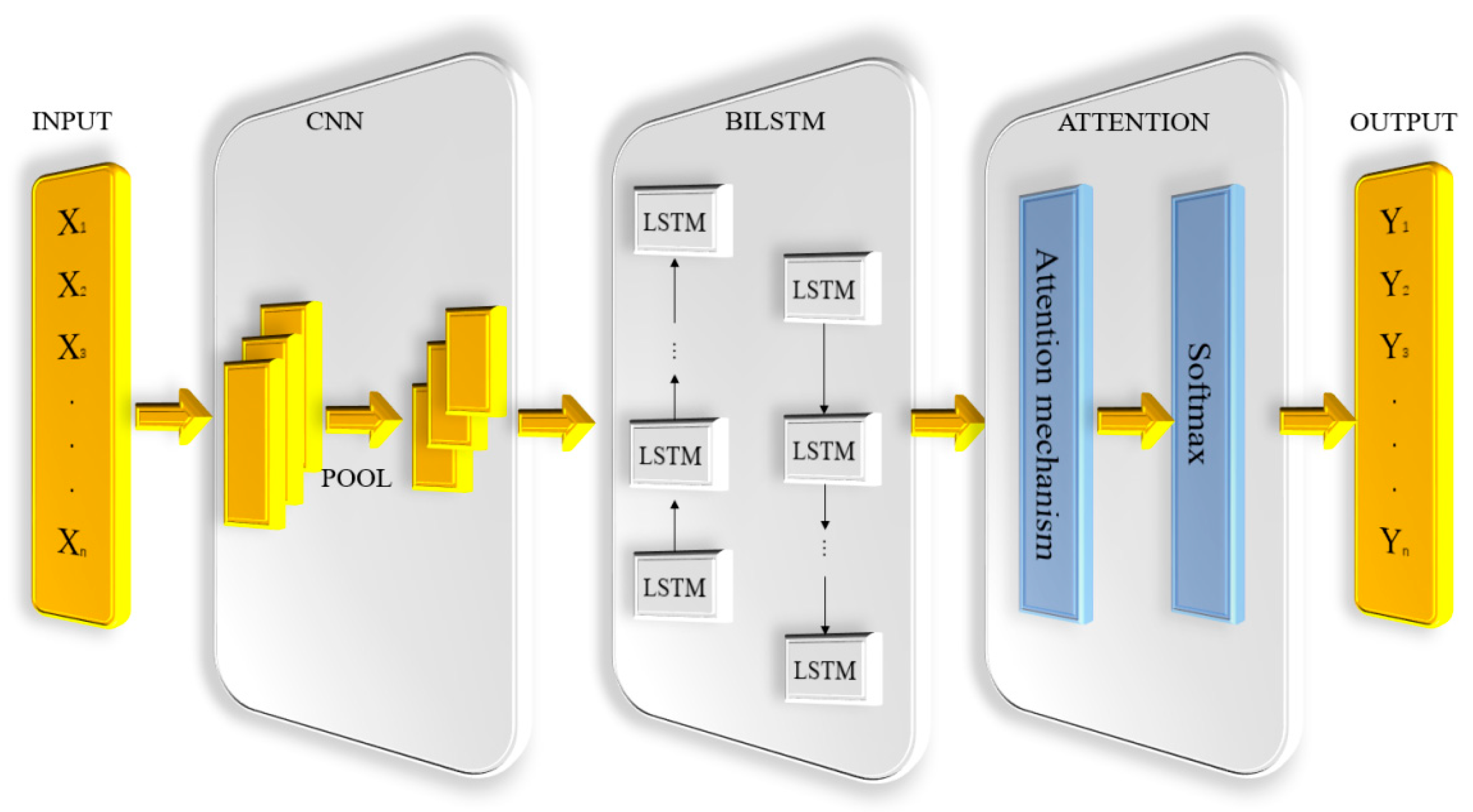
The CNN–BiLSTM–Attention model has a three-stage cascaded structure. Data flows sequentially from the input layer to the CNN feature extraction layer, BiLSTM sequence modeling layer, attention weighting layer, and then to the output layer. Core logic is as follows: first, local discriminative feat from raw data, then model temporal/spatial dependencies of the local feat, and lastly highlight important feat components to focus the model on the most important info. The overall architecture of the entire system is shown in Figure 3.

4.2. Detailed Design of Each Part

Convolutional Neural Networks are among the most frequently used algorithms in deep learning. Due to their good feature extraction ability, they have been used in pavement performance studies. The main components of CNNs are convolutional layers and pooling layers. The convolutional layer obtains the effective nonlinear local features of the input data with convolution kernels, and the pooling layer further compresses the output features of the convolutional layer to acquire more key feature information to enhance the generalization ability [37]. This addresses the problem of low efficiency of BiLSTM in extracting local patterns from long sequences. The core architecture design and implementation principles are as follows:

Multi-scale convolutional feature extraction: This study employs 1D convolutional layers to construct a multi-scale feature-perception module. By setting convolution kernels with different window sizes, the network can systematically acquire cross-scale local feature patterns in the input sequence data. Each convolution kernel does a sliding convolution operation along the sequence-length dimension. The number of output channels is defined as a tunable hyperparameter to adjust the richness of the feature extraction and model complexity.

Convolutional Layer 1: Uses 32 convolutional filters with a kernel size of [1, 1], a default stride of [1, 1], and valid padding (no zero-padding). The output feature map dimension is adjusted to 32 channels.

Activation function: After the convolution operation, the ReLU (rectified linear unit) function is used to introduce nonlinearity, which helps the model learn more complex feature mappings. The ReLU function is defined as

$$\mathrm{f}\left(\mathrm{x}\right)=\max \left(0, \mathrm{x}\right)$$

(10)

Convolutional Layer 2: Follows the ReLU layer with 64 convolutional filters of size [1, 1] (stride = [1, 1], valid padding), expanding the feature dimension to 64 channels.

Max pooling: After convolution, max pooling is performed on each output channel (for example, 1D max pooling, and the pool size is equal to the length of the convolution output) to retain the most discriminative local features (i.e., the maximum value in each feature map) and reduce the dimensionality of the feature tensor in order to prevent overfitting and speed up the subsequent BiLSTM computation.

$$\mathrm{p} (\mathrm{F}) =\max {\mathrm{F}}_{\mathrm{i}}$$

(11)

where F is the feature-map vector. By keeping the local maximum activation responses, this mechanism reduces the feature dimensionality and retains the most discriminative feature patterns. This design not only effectively avoids the problem of overfitting, but also greatly improves the computational efficiency by lowering the input dimensionality of the following BiLSTM module.

BiLSTM layer sequence-dependency modeling: LSTM only depends on past sequence information for prediction at the next time step. A problem is raised: the present time step’s output is associated not only with previous information, but also with future information [38]. BiLSTM was therefore connected by adding two LSTMs to the architecture to combine the past and future information for the current time step to effectively improve the prediction accuracy. The calculation process for the forward propagation and backward propagation states of a BiLSTM network is as follows:

Forward LSTM

Input sequence: x₁, x₂, …, x_t; output hidden-state sequence: h₁^f, h₂^f, …, h_t^f.

Gate calculations:

$${\mathrm{i}}_{\mathrm{t}}^{\mathrm{f}} = \mathsf{\sigma }({\mathrm{W}}_{\mathrm{i}}^{\mathrm{f}}{\mathrm{x}}_{\mathrm{t}} + {\mathrm{U}}_{\mathrm{i}}^{\mathrm{f}}{\mathrm{h}}_{\mathrm{t}-1}^{\mathrm{f}} + {\mathrm{b}}_{\mathrm{i}}^{\mathrm{f}}) (\mathrm{Input} \mathrm{gate})$$

(12)

$${\mathrm{f}}_{\mathrm{t}}^{\mathrm{f}}=\mathsf{\sigma }({\mathrm{W}}_{\mathrm{f}}^{\mathrm{f}}{\mathrm{x}}_{\mathrm{t}}+{\mathrm{U}}_{\mathrm{f}}^{\mathrm{f}}{\mathrm{h}}_{\mathrm{t}-1}^{\mathrm{f}}+{\mathrm{b}}_{\mathrm{f}}^{\mathrm{f}}) (\mathrm{Forget} \mathrm{gate})$$

(13)

$${\mathrm{o}}_{\mathrm{t}}^{\mathrm{f}}=\mathsf{\sigma }({\mathrm{W}}_{\mathrm{o}}^{\mathrm{f}}{\mathrm{x}}_{\mathrm{t}}+{\mathrm{U}}_{\mathrm{o}}^{\mathrm{f}}{\mathrm{h}}_{\mathrm{t}-1}^{\mathrm{f}}+{\mathrm{b}}_{\mathrm{o}}^{\mathrm{f}}) (\mathrm{Output} \mathrm{gate})$$

(14)

$${\mathrm{g}}_{\mathrm{t}}^{\mathrm{f}}=\tan \mathrm{h}({\mathrm{W}}_{\mathrm{c}}^{\mathrm{f}}{\mathrm{x}}_{\mathrm{t}}+{\mathrm{U}}_{\mathrm{c}}^{\mathrm{f}}{\mathrm{h}}_{\mathrm{t}-1}^{\mathrm{f}}+{ \mathrm{b}}_{\mathrm{c}}^{\mathrm{f}}) (\mathrm{Candidate} \mathrm{cell} \mathrm{state})$$

(15)

Cell state update:

$${\mathrm{c}}_{\mathrm{t}}^{\mathrm{f}} = {\mathrm{c}}_{\mathrm{t}}^{\mathrm{f}} \odot {\mathrm{c}}_{\mathrm{t}-1}^{\mathrm{f}}+{\mathrm{i}}_{\mathrm{t} }^{\mathrm{f}}\odot { \mathrm{g}}_{\mathrm{t}}^{\mathrm{f}}$$

(16)

Hidden state output:

$${\mathrm{h}}_{\mathrm{t}}^{\mathrm{f}} ={ \mathrm{o}}_{\mathrm{t}}^{\mathrm{f}} \odot \tan \mathrm{h} \left({\mathrm{c}}_{\mathrm{t}}^{\mathrm{f}}\right)$$

(17)

Backward LSTM

Input reversed sequence: x_t, x_t−1, …, x₁; output hidden-state sequence: h_t^b, h_t−1^b, …, h₁^b.

Gate calculations:

$${\mathrm{i}}_{\mathrm{t}}^{\mathrm{b}} = \mathsf{\sigma }({\mathrm{W}}_{\mathrm{i}}^{\mathrm{b}}{\mathrm{x}}_{\mathrm{t}}+{\mathrm{U}}_{\mathrm{i}}^{\mathrm{b}}{\mathrm{h}}_{\mathrm{t}+1}^{\mathrm{b}}+{\mathrm{b}}_{\mathrm{i}}^{\mathrm{b}}) (\mathrm{Input} \mathrm{gate})$$

(18)

$${\mathrm{f}}_{\mathrm{t}}^{\mathrm{b}}=\mathsf{\sigma }({\mathrm{W}}_{\mathrm{f}}^{\mathrm{b}}{\mathrm{x}}_{\mathrm{t}}+{\mathrm{U}}_{\mathrm{f}}^{\mathrm{b}}{\mathrm{h}}_{\mathrm{t}+1}^{\mathrm{b}}+{\mathrm{b}}_{\mathrm{f}}^{\mathrm{b}}) (\mathrm{Forget} \mathrm{gate})$$

(19)

$${\mathrm{o}}_{\mathrm{t}}^{\mathrm{b}}=\mathsf{\sigma }({\mathrm{W}}_{\mathrm{o}}^{\mathrm{b}}{\mathrm{x}}_{\mathrm{t}}+{\mathrm{U}}_{\mathrm{o}}^{\mathrm{b}}{\mathrm{h}}_{\mathrm{t}+1}^{\mathrm{b}}+{\mathrm{b}}_{\mathrm{o}}^{\mathrm{b}}) (\mathrm{Output} \mathrm{gate})$$

(20)

$${\mathrm{g}}_{\mathrm{t}}^{\mathrm{b}}=\tan \mathrm{h}({\mathrm{W}}_{\mathrm{c}}^{\mathrm{b}}{\mathrm{x}}_{\mathrm{t}}+{\mathrm{U}}_{\mathrm{c}}^{\mathrm{b}}{\mathrm{h}}_{\mathrm{t}+1}^{\mathrm{b}}+{\mathrm{b}}_{\mathrm{c}}^{\mathrm{b}}) (\mathrm{Candidate} \mathrm{cell} \mathrm{state})$$

(21)

Cell state update:

$${\mathrm{c}}_{\mathrm{t}}^{\mathrm{b}} = {\mathrm{c}}_{\mathrm{t}}^{\mathrm{b}} \odot {\mathrm{c}}_{\mathrm{t}+1}^{\mathrm{b}}+{\mathrm{i}}_{\mathrm{t}}^{\mathrm{b}} \odot {\mathrm{g}}_{\mathrm{t}}^{\mathrm{b}}$$

(22)

Hidden state output:

$${\mathrm{h}}_{\mathrm{t}}^{\mathrm{b}} ={ \mathrm{o}}_{\mathrm{t}}^{\mathrm{b}}\odot \tan \mathrm{h} \left({\mathrm{c}}_{\mathrm{t}}^{\mathrm{b}}\right)$$

(23)

Bidirectional output merging:

$${\mathrm{h}}_{\mathrm{t}} = \mathrm{concat}({\mathrm{h}}_{\mathrm{t}}^{\mathrm{f}},{\mathrm{h}}_{\mathrm{t}}^{\mathrm{b}}) = [{\mathrm{h}}_{\mathrm{t}}^{\mathrm{f}};{\mathrm{h}}_{\mathrm{t}}^{\mathrm{b}}]$$

(24)

where W, U, and b: trainable parameters (weight matrices and biases);

σ: Sigmoid activation function;

tanh: hyperbolic tangent activation function;

⊙: element-wise multiplication;

concat: vector concatenation.

In the implementation, the BiLSTM module is used to capture temporal dependencies in the calibrated features. First, the folded sequence is restored through the Sequence Unfolding Layer, where the mini-batch size information from the sequence folding layer is used to ensure dimensional consistency. Then, the Flatten Layer converts the 3-dimensional feature map into a 1-dimensional vector to match the input format of the BiLSTM layer. The BiLSTM layer is configured with one bidirectional LSTM layer that contains 6 neurons in each direction (12 hidden units in total). The output mode is set to “last”, meaning only the hidden state of the last time step is retained for subsequent regression tasks. Moreover, the sequence length of the BiLSTM layer is equal to the input feature dimension, as the feature vector of each sample is treated as a sequence with a length consistent with the input feature dimension. Moreover, the sequence length of the BiLSTM layer is equal to the input feature dimension f_, as the feature vector of each sample is treated as a sequence of length f_.

Attention-layer key-feature weighting: Drawing on the selective attention mechanism of human visual cognition, this component enables targeted acquisition of pivotal information and elimination of redundant, non-critical data. Through the allocation of probabilistic weights, it guides the neural network to focus on specific feature categories, which in turn contributes to the improvement of prediction outcomes [39]. Also, it reduces the information loss caused by sequences that are too long in the BiLSTM layer. So, introducing an attention mechanism into a neural network may also improve the prediction accuracy of the neural network [40].

A Squeeze-and-Excitation (SE) Attention mechanism was adopted to adaptively recalibrate the channel-wise feature weights, enhancing the model’s focus on critical features:

Squeeze Operation: The global average pooling output (64-dimensional vector) is fed into a fully connected layer with 16 neurons, reducing the feature dimension to 16 to capture channel-wise dependencies.

Excitation Operation: A ReLU activation function is applied to the compressed vector, followed by another fully connected layer that maps the 16-dimensional vector back to 64 dimensions. A Sigmoid activation function is then used to generate attention weights (ranging from 0 to 1) for each of the 64 channels.

Feature Calibration: The attention weights are multiplied element-wise with the original 64-channel feature map from the CNN module (via multiplication layer), emphasizing important channels and suppressing irrelevant ones.

Note: The SE Attention mechanism focuses on channel-wise feature refinement. Its core dimensions are defined as the compression dimension (16) and the recovery dimension (64), which correspond to the number of neurons in the two fully connected layers.

4.3. Model Training Strategy

The model was trained using MATLABR 2023b’s Deep Learning Toolbox, using the following key hyperparameters and training settings:

Optimizer: Adam optimizer, which adaptively adjusts the learning rate for each parameter using first-order and second-order moment estimates, improving training stability and convergence speed.

Initial Learning Rate: Set to 0.01. A piecewise learning rate schedule was adopted, with a drop factor of 0.1 and a drop period of 500 epochs (i.e., the learning rate is reduced to 0.001 after 500 training epochs). All other models adopt this hyperparameter configuration.

Training Epochs: The maximum number of training epochs (MaxEpochs) was set to 500 to ensure sufficient model training without overfitting.

Batch Size: The batch size was set to the default value of MATLAB’s trainNetwork function (typically 128 for small- to medium-sized datasets), balancing training efficiency and memory usage.

Loss Function: The mean squared error (MSE) was used as the loss function, which is suitable for regression tasks to minimize the squared difference between predicted and true values.

Regularization: No L1/L2 regularization or dropout was applied in this study as the model’s generalization ability was ensured through data shuffling and the train–test split.

Data Shuffling: The training set was shuffled every epoch (Shuffle = ‘every-epoch’) to prevent the model from memorizing the training sequence.

Training Visualization: The ‘Plots’ = ‘training-progress’ option was enabled to display real-time training curves (loss vs. epochs) to monitor convergence.

5. Results and Discussion

5.1. Results

5.1.1. Quantitative Results of Model Prediction Performance

Based on 2067 sets of measured asphalt pavement performance data of national and provincial trunk highways in Xinjiang from 2020 to 2024, this study took 4 years of historical PCI and RQI data as input to predict the fifth-year indicators. The CNN–BiLSTM–Attention model was quantitatively validated against four comparison models: RF, CNN, LSTM, and CNN–LSTM–Attention. Three core indicators, R², MAE, and MBE, were adopted to evaluate the model’s goodness of fit, absolute error, and systematic bias. The prediction results of each model for PCI and RQI are shown in

Table 8. Comparison of PCI prediction results.

Model	R2	MAE	MBE
RF	0.784	9.51	−2.1
CNN	0.823	5.77	0.72
LSTM	0.821	5.63	−0.39
CNN–LSTM–Attention	0.817	5.34	0.81
CNN–BiLSTM–Attention	0.837	5.31	0.11

and

Table 9. Comparison of RQI prediction results.

Model	R2	MAE	MBE
RF	0.846	1.95	0.21
CNN	0.828	2.02	0.23
LSTM	0.761	2.68	−0.76
CNN–LSTM–Attention	0.737	2.53	0.73
CNN–BiLSTM–Attention	0.855	1.84	0.47

, and the radar comparison charts for model performance are presented in Figure 4 and Figure 5.

According to the comparative results presented in Table 8 and Table 9, the proposed CNN–BiLSTM–Attention model exhibited superior predictive performance for both PCI and RQI. For PCI prediction, the model attained an R² of 0.837, representing a 1.7% improvement over the second-best performer (the CNN model). Furthermore, the MAE was reduced to 5.31—a 0.57% decrease relative to the CNN–LSTM–Attention architecture—while its MBE of 0.11 indicated negligible systematic bias. In terms of RQI prediction, the R² reached 0.855, surpassing the Random Forest (RF) model by 1.1%, while the MAE was 1.84, marking a significant 5.6% reduction compared to RF. Although its MBE was marginally higher than those of the RF and CNN models, the proposed framework maintained the most robust overall error mitigation. The radar chart analysis further corroborates these findings, demonstrating that the proposed model excels across all evaluation metrics without discernible deficiencies, thereby underscoring its reliability and precision in short-time-series forecasting of asphalt pavement performance.

5.1.2. Fitting Characteristics of Predicted and Measured Values

Scatter fitting plots of the predicted and measured values of PCI and RQI by the CNN–BiLSTM–Attention model were plotted (Figure 6, Figure 7, Figure 8, Figure 9 and Figure 10). The results showed that the scatter points of the predicted and measured values of PCI and RQI were highly concentrated on both sides of the ideal fitting line with no obvious discrete points or outliers. The fitting degree of scatter points for PCI prediction reached 83.7% and 85.5% for RQI, indicating that the model can effectively capture the deterioration trend and numerical characteristics of pavement performance and has a good fitting effect on the annual change prediction of pavement performance. Meanwhile, the model had no obvious prediction bias in the low-value range of PCI (<60) and the middle-value range of RQI (90–95), solving the problem of insufficient prediction accuracy of traditional models in the characteristic intervals of indicators and providing reliable quantitative data support for engineering maintenance decision-making.

Random forest (RF) model:

Figure 6. PCI and RQI from RF model.

Figure 6. PCI and RQI from RF model.

CNN pavement performance prediction model:

Figure 7. PCI and RQI from CNN model.

Figure 7. PCI and RQI from CNN model.

LSTM pavement performance prediction model:

Figure 8. PCI and RQI from LSTM model.

Figure 8. PCI and RQI from LSTM model.

CNN–LSTM–Attention pavement performance prediction model:

Figure 9. PCI and RQI from CNN–LSTM–Attention model.

Figure 9. PCI and RQI from CNN–LSTM–Attention model.

CNN–BiLSTM–Attention pavement performance prediction model:

Figure 10. PCI and RQI from CNN–BiLSTM–Attention model.

Figure 10. PCI and RQI from CNN–BiLSTM–Attention model.

It can be seen that the CNN–BiLSTM–Attention model has good stability and performance across different indices in the prediction tasks. By using CNN feature extraction, Bidirectional LSTM to capture the bidirectional dependency of sequence data, and Attention to focus on key information, the model is better at meeting the scenario requirements and is the most reliable model for the considered prediction tasks Figure 11 and Figure 12 show the distribution of predicted and actual values.

6. Discussion

6.1. Integrated Application of Prediction Results and Engineering Maintenance Standards

The predictive outputs of this study are directly aligned with the Specifications for Design and Maintenance of Highway Asphalt Pavements (JTG 5421-2018), providing a quantitative framework for hierarchical prioritization and strategy selection in pavement management. This alignment facilitates the operationalization of a “data-to-decision” workflow. Specifically, the model outputs longitudinal performance gradations for discrete road segments, enabling engineers to map predicted condition states and link them directly to standardized maintenance protocols. This approach clarifies the optimal timing, specific measures, and priority levels for intervention, thereby supplanting conventional maintenance paradigms characterized by heuristic judgment and reactive implementation. Consequently, this study establishes a systematic, quantitative, and proactive decision-making framework that significantly optimizes the allocation and utilization of maintenance resources in resource-constrained environments.

6.2. Comparative Analysis with Previous Studies and Core Contributions of This Study

To clarify the innovative value and academic contributions of this study, the results of this study were compared with those of representative studies in the field of pavement performance prediction in recent years from multiple dimensions, focusing on four aspects: modeling data dependence, prediction time-series length, core indicator R², and engineering adaptability, as shown in

Table 10. Comparative analysis of this study and representative recent studies.

Authors	Modeling Method	Modeling Data Type	Prediction Time-Series Length	R2 of PCI/RQI-Like Indicators	Engineering Adaptable Scenario
Guo et al. (2021) [15]	LSTM–Attention	PCI + Climate + Traffic Load	10-year long time series	0.812	High-grade highways in eastern developed regions
Cai et al. (2023) [16]	CTGCN	IRI + Environment + Pavement Structural Parameters	6-year time series	0.825	Urban arterial roads with complete data
Li et al. (2022) [17]	PSO-GRU	PCI + RQI + Traffic Load	8-year time series	0.809	Expressway network
This Study (2025)	CNN–BiLSTM–Attention	Only PCI/RQI Single-Source Performance Data	4-year short time series	PCI: 0.837/RQI: 0.855	National and provincial trunk highways in resource-constrained western regions

.

The comparative analysis demonstrates significant advancements in low-dependency, short-time-series modeling for remote regions, with the core contributions spanning both scientific theory and engineering practice.

Scientific Contributions: This study validates a single-source data modeling approach that captures nonlinear bidirectional dependencies in short-time-series pavement data. It introduces an optimized CNN–BiLSTM–Attention framework that overcomes feature sparsity in small-sample scenarios, achieving superior predictive accuracy (R² > 0.83) compared to state-of-the-art models.

Engineering Contributions: The proposed method provides a cost-effective solution for resource-constrained regions by requiring only four years of historical data for accurate forecasting. By aligning predictions with national maintenance standards, it enables a transition from reactive to preventative maintenance, offering a lightweight, deployable tool for regional highway management.

6.3. Research Limitations and Risk Analysis

While the proposed CNN–BiLSTM–Attention framework demonstrated high predictive accuracy for short-term pavement performance, several limitations and operational risks must be critically acknowledged:

The model only uses PCI and RQI for prediction without considering climate, traffic load and pavement structure. Its accuracy may decline under extreme conditions, and it cannot capture sudden performance changes caused by extreme events.

All data are from Xinjiang, which is dry with large temperature differences and low traffic. The model may not be directly applicable to rainy or heavy-traffic areas in eastern China.

The model is designed for 4-year time series. When the time series is shorter than 3 years, the prediction accuracy will decrease significantly, so it is not suitable for new roads.

6.4. Correlative Contributions to the Field of Architectural Science

As a cross-disciplinary integration of road engineering and deep learning, this study offers significant reference value and scalability for infrastructure performance prediction within the broader field of architectural science. A primary objective of architectural science is the realization of intelligent life-cycle management for infrastructure. As a cornerstone of transportation systems, the proposed pavement performance prediction methodology serves as a viable template for other infrastructure types, such as bridges, tunnels, and municipal networks: ① The data-efficient deep learning approach developed herein can be applied to scenarios characterized by a scarcity of multi-source data, including bridge deflection monitoring and tunnel lining degradation. ② The hybrid architecture of “feature extraction–time-series modeling–key weighting” establishes a robust methodological blueprint for time-series performance forecasting. ③ The integrated framework of “prediction results–engineering standards–decision guidance” provides a replicable model for engineering implementation, advancing architectural science toward data-driven, intelligent decision-making.

7. Conclusions

Addressing the scientific and engineering challenges of asphalt pavement performance prediction for trunk highways in resource-constrained regions, this study develops a data-efficient prediction method based on a CNN–BiLSTM–Attention architecture. Validated using 2067 sets of empirical data from Xinjiang, the model facilitates the integrated application of predictive analytics and engineering maintenance standards. The main conclusions are as follows.

7.1. Core Scientific Achievements

Elucidation of Short-Term Deterioration Laws: The study reveals that annual changes in the Pavement Condition Index (PCI) and Riding Quality Index (RQI) of trunk highways in Xinjiang exhibit significant self-similarity and nonlinear bidirectional temporal correlations. Four years of historical performance data are sufficient to characterize deterioration trends without necessitating multi-source variables (e.g., climate or traffic load), providing a theoretical foundation for data-efficient pavement modeling.

Optimization of Hybrid Architectures: A CNN–BiLSTM–Attention hybrid framework optimized for 4-year short time series was developed. A 1D-CNN extracts local deterioration features, the BiLSTM captures bidirectional temporal dependencies, and the Attention mechanism weights critical deterioration nodes. This architecture achieves synergistic optimization, overcoming the limitations of insufficient feature mining and poor generalization that are inherent in traditional models when applied to small-sample scenarios.

Enhanced Predictive Accuracy: The proposed model achieved R² values of 0.837 and 0.855 for PCI and RQI prediction, respectively, with systematic biases (MBE) approaching zero. It consistently outperformed mainstream models such as Random Forest (RF), CNN, and LSTM, establishing a high-precision technical path for time-series pavement performance forecasting.

7.2. Key Engineering Achievements

Development of a Resource-Efficient Methodology: The model enables accurate fifth-year performance forecasting using only four years of single-source data (PCI/RQI). This reduces the data collection and processing workload for engineering technicians by over 80%, effectively resolving the bottleneck of multi-source data scarcity in remote regions.

Integration with Maintenance Standards: By aligning predictive outputs with the Technical Standard for Highway Condition Evaluation (JTG 5210-2018), the framework allows for the direct determination of maintenance priorities and schedules. This facilitates a transition from experience-based judgment to quantitative, data-driven decision-making, optimizing maintenance resource allocation.

Validation of Operational Feasibility: Given its streamlined architecture and low computational overhead, the model is suitable for direct deployment within local-level highway management systems. Pilot implementations on Xinjiang trunk highways have demonstrated robust engineering performance and high potential for broader deployment.

7.3. Explicit Applicable Conditions of the Model

To ensure engineering reliability, the CNN–BiLSTM–Attention model must be applied within the following boundary conditions:

Data Requirements: A minimum of three years of measured annual PCI/RQI data is required, with a sample size of N ≥ 500 and no significant outliers.

Regional Constraints: The model is calibrated for asphalt pavements on Class II, III, and IV highways in arid and semi-arid regions characterized by moderate traffic and low precipitation.

Operational Constraints: Performance should be within normal operational limits, excluding sections affected by geological disasters, sudden extreme loading, or anthropogenic damage.

Temporal Scope: The model is optimized for “4-year-to-5th-year” annual forecasting and is not intended for monthly/daily intervals or decadal long-term projections.

7.4. Specific Future Research Directions

Multi-Source Data Fusion: Future iterations will incorporate climatic variables (temperature, and precipitation) and structural parameters to enhance the model’s robustness in predicting performance fluctuations under extreme environmental stressors.

Cross-Regional Adaptability: Utilizing transfer learning, the model will be fine-tuned using datasets from high-precipitation and high-traffic density regions (e.g., Eastern China) to develop a generalized cross-regional prediction framework.

Lightweight Edge Deployment: Research will focus on pruning model parameters to facilitate deployment on edge-computing terminals, enabling real-time, on-site pavement performance assessment for field units.

Coupling Performance and Cost Optimization: By integrating maintenance cost data, future research aims to establish a unified “performance prediction–maintenance decision–cost optimization” model to maximize the lifecycle value of transportation infrastructure.