Risk Assessment Indicator Weighting for Deep Foundation Pit Construction Using Dual Probabilistic Linguistic Term Sets

Abstract

In deep foundation pit risk assessment, expert ratings are often aggregated without preserving the dispersion of individual opinions, yet such dispersion directly reflects the reliability of the assessment. To address this shortcoming, this study integrates dual probabilistic linguistic term sets (DPLTS), entropy theory, and the best–worst method (BWM). In this DPLTS framework, the membership set L(p) encodes the central tendency of expert ratings (the assessed risk level), while the non-membership set U(q) encodes the dispersion of ratings, serving as a proxy for expert disagreement—a source of uncertainty that is as critical as the risk level itself for decision-making. The least common multiple expansion method standardizes information length. Secondary indicator weights are determined using fuzzy entropy and cross-entropy, while primary indicator weights are derived via BWM, forming a combined subjective-objective weighting model. Hierarchical aggregation yields the overall risk expectation value. A case study assesses the project as Level III (moderate) risk, with a low variance of 0.0503 indicating strong expert consensus. The risk expectation varies by less than 4% under different entropy measures, confirming robustness. Comparative analysis with fuzzy comprehensive evaluation and CRITIC–Grey system methods shows consistent results, with all three identifying excavation and support as key risk indicators. The proposed method provides not only a reliable risk level but also a quantitative measure of expert agreement, offering enhanced support for targeted risk management.

1. Introduction

Accelerated urbanization in China has made deep excavation projects a critical component of underground space development [1,2]. These projects are often situated in dense urban environments with complex utility networks and variable geological conditions, exposing construction to multiple risks, including instability of supporting structures, excavation collapse, and ground settlement. Should these risks materialize, they can lead to substantial economic losses and significant social impact [3,4]. Consequently, accurately assessing the risk level of deep excavation and identifying the key risk indicators are of great practical importance for proactive risk management and engineering safety [5,6].

Existing research on risk assessment for deep excavation has primarily focused on constructing indicator systems, determining indicator weights, and integrating assessment models. For instance, Chen et al. [7] developed a collapse risk model using variable fuzzy set theory, enhancing scientific rigor through combined subjective and objective weighting. Fu et al. [8] adopted a risk propagation perspective, employing association rules [9] and an improved SIR model to uncover the dynamic interactions among risk factors in complex projects. Xu et al. [10] integrated the CRITIC method with grey system theory to reduce subjective bias while better accounting for inter-indicator relationships. Gong et al. [11] proposed an ensemble classification model to effectively tackle imbalanced data and enhance the safety risk evaluation of deep foundation construction schemes. Other approaches include combining AHP with extension theory [12], applying multi-source information fusion and deep learning for dynamic assessment [13,14], utilizing fuzzy extension models for multi-attribute information [15,16], and employing fuzzy evidence reasoning for scenarios with incomplete information [17]. While these methods have advanced the objectivity, systematic nature, and applicability of risk assessment, common limitations persist. These include inadequate representation of uncertain information, limited discrimination in weight assignment, and insufficient capture of expert hesitation, which collectively hinder the precise identification of critical risk factors.

Recent years have seen the emergence of tools capable of more precisely capturing expert hesitation [18,19]. Torra [20] introduced the hesitant fuzzy set, which allows membership degrees to have multiple possible values. Zhu et al. [21] advanced this concept to the probabilistic hesitant fuzzy set by assigning probabilities to each membership degree. In the realm of linguistic information, the probabilistic linguistic term set (PLTS) proposed by Pang et al. [22], which combines linguistic terms with probability distributions, has become a focal point of research. However, the PLTS describes information only from the single dimension of “support/membership.” This proves insufficient for expressing the complex, dialectical psychology often encountered in risk assessment, such as simultaneous but opposing tendencies to rate a risk as both “high” and “low.” To address this, Xie et al. [23] proposed the double-sided probabilistic linguistic term set (DPLTS). By concurrently considering probabilistic linguistic information for both membership and non-membership, the DPLTS provides a more comprehensive mathematical tool for modeling the bipolar hesitation inherent in expert judgment [24,25,26,27].

Consider two hypothetical risk indicators. Both receive the same average expert rating, but one has tightly clustered scores while the other shows wide dispersion. Aggregating ratings without preserving this dispersion would treat both indicators as equally reliable, yet the latter indicates substantial expert disagreement—a source of uncertainty that directly affects decision confidence. Against this backdrop, this study proposes a risk rating method for deep excavation projects based on the DPLTS. The method converts expert evaluations into DPLTS form to capture both the central risk tendency (membership set) and the degree of expert disagreement (non-membership set). The least common multiple extension method standardizes the information length. Fuzzy entropy and cross-entropy determine objective weights for secondary indicators, while the best–worst method (BWM) provides subjective weights for primary indicators, forming a combined weighting model. Hierarchical aggregation yields the overall risk expectation value, which is then mapped to a risk level. The outputs—risk level, indicator weights, and per-indicator variance—are explicitly linked to engineering decisions: the risk level determines the required management attention and monitoring frequency; the weights guide resource prioritization; and the variance flags indicators that need additional expert review or field verification. This design directly responds to the critique that assessment models can be “method-driven rather than problem-driven” by ensuring every analytical output has a clear engineering interpretation. A case study and comparative analysis validate the effectiveness of the proposed method in delivering actionable insights for deep excavation risk management.

2. Materials and Methods

2.1. Double-Sided Probabilistic Linguistic Term Set (DPLTS)

In multi-criteria evaluation, experts often prefer to express their judgments using natural language. The Probabilistic Linguistic Term Set (PLTS) is a common tool for representing such uncertain information, as it can describe an expert’s assessment of the degree of membership for a given criterion along with its probability distribution. However, the PLTS reflects information from only a single perspective (membership), making it difficult to fully capture the hesitation and complexity inherent in evaluations. In contrast, the Double-Sided Probabilistic Linguistic Term Set (DPLTS) provides a structured format to encode both the evaluated risk level (via the membership set) and the degree of disagreement among experts (via the non-membership set). This dual-output capability allows decision-makers to not only obtain an overall risk expectation but also to assess the reliability of that expectation based on the level of expert consensus.

Definition 1.

Let X be a non-empty finite universe of discourse. A Double-Sided Probabilistic Linguistic Term Set (DPLTS) on X is defined as:

$$\mathrm{D}=\left\{〈\mathrm{x},\mathrm{L}\left(\mathrm{p}\right),\mathrm{U}\left(\mathrm{q}\right)〉|\mathrm{x}\in \mathrm{X}\right\}$$

(1)

where

$\mathrm{L}\left(\mathrm{p}\right)=\left\{{\mathrm{L}}^{\left(\mathrm{i}\right)}\left({\mathrm{p}}^{\left(\mathrm{i}\right)}\right)|{\mathrm{L}}^{\left(\mathrm{i}\right)}\in \mathrm{S},{\mathrm{p}}^{\left(\mathrm{i}\right)}\ge 0,{\sum }_{\mathrm{k}=1}^{\#\mathrm{L}\left(\mathrm{p}\right)}{\mathrm{p}}^{\left(\mathrm{i}\right)}\le 1\right\}$ is termed the membership degree set, expressing the probabilistic linguistic evaluation of element x belonging to a defined fuzzy concept.

$\mathrm{U}\left(\mathrm{q}\right)=\left\{{\mathrm{U}}^{\left(\mathrm{j}\right)}\left({\mathrm{q}}^{\left(\mathrm{j}\right)}\right)|{\mathrm{U}}^{\left(\mathrm{j}\right)}\in \mathrm{S},{\mathrm{q}}^{\left(\mathrm{j}\right)}\ge 0,{\sum }_{\mathrm{j}=1}^{\#\mathrm{U}\left(\mathrm{q}\right)}{\mathrm{q}}^{\left(\mathrm{j}\right)}\le 1\right\}$ is termed the non-membership degree set, expressing the probabilistic linguistic evaluation of element x not belonging to that fuzzy concept.

$\mathrm{S}=\left\{{\mathrm{s}}_{\mathsf{\alpha }}|\mathsf{\alpha }=-\mathsf{\tau },\cdots ,0,\cdots ,\mathsf{\tau }\right\}$ is a symmetrical, ordered, discrete linguistic term set, where τ is a positive integer that represents the granularity of the linguistic terms. This definition is general and applicable to linguistic evaluation systems of any granularity. #L(p) and #U(p) denote the number of elements in the membership degree set and non-membership degree set, respectively.

$\mathrm{D}=〈\mathrm{L}\left(\mathrm{p}\right),\mathrm{U}\left(\mathrm{p}\right)〉$ is called a Double-sided Probabilistic Linguistic Element (DPLE), which serves as the fundamental unit of a DPLTS. In group evaluation, a single DPLE can represent the collective assessment of an expert panel regarding a specific alternative under a given criterion.

2.2. Least Common Multiple-Based Extension Method for Hesitant Fuzzy Elements

In risk level assessment, differences in expert knowledge often lead to DPLTS evaluations for the same criterion that contain different numbers of elements (i.e., different set lengths) in both the membership degree set L(p) and the non-membership degree set U(q). DPLTS with such inconsistent cardinalities cannot be directly used in precise mathematical operations, such as calculating distance, similarity, or information aggregation.

Consider two Double-sided Probabilistic Linguistic Elements (DPLEs) to be compared: ${\mathrm{D}}_1=〈{\mathrm{L}}_1\left(\mathrm{p}\right),{\mathrm{U}}_1\left(\mathrm{q}\right)〉$ and ${\mathrm{D}}_2=〈{\mathrm{L}}_2\left(\mathrm{p}\right),{\mathrm{U}}_2\left(\mathrm{q}\right)〉$.

Step 1: Determine the Length via Least Common Multiple

Calculate the least common multiple (LCM) for the lengths of the membership degree set and the non-membership degree set, respectively:

$${\mathrm{l}}_{\mathrm{h}}=\mathrm{l}\mathrm{c}\mathrm{m}\left(\#{\mathrm{L}}_1\left(\mathrm{p}\right),\#{\mathrm{L}}_2\left(\mathrm{p}\right)\right)$$

(2)

$${\mathrm{l}}_{\mathrm{g}}=\mathrm{l}\mathrm{c}\mathrm{m}\left(\#{\mathrm{U}}_1\left(\mathrm{q}\right),\#{\mathrm{U}}_2\left(\mathrm{q}\right)\right)$$

(3)

where lcm(a, b) denotes the least common multiple of the integers a and b.

Step 2: Construct the Extended DPLTS

Each DPLTS is extended to the unified length by replicating the elements from its original set and evenly redistributing their corresponding probabilities. For the membership degree set ${\mathrm{L}}_1\left(\mathrm{p}\right)$ of ${\mathrm{D}}_1$, the extended set ${\mathrm{L}}_1\left(\mathrm{p}\right)$ is defined as:

$$\overline{{\mathrm{L}}_1}\left(\mathrm{p}\right)=\left\{\left({\mathrm{L}}_1^{\left(\mathsf{\kappa }\right)},{\overline{{\mathrm{p}}_1}}^{\left(\mathsf{\kappa }\right)}\right)|\mathsf{\kappa }=\mathrm{1,2},\cdots ,{\mathrm{l}}_{\mathrm{h}}\right\}$$

The elements and their adjusted probabilities are given by:

$${\mathrm{L}}_1^{\left(\mathsf{\kappa }\right)}={\mathrm{L}}_1^{\left(\mathrm{i}\right)},{\overline{{\mathrm{p}}_1}}^{\left(\mathsf{\kappa }\right)}={\displaystyle \frac{{\mathrm{p}}_1^{\left(\mathrm{i}\right)}}{\frac{{\mathrm{l}}_{\mathrm{h}}}{{\mathrm{L}}_1\left(\mathrm{p}\right)}}}\mathrm{f}\mathrm{o}\mathrm{r}\mathsf{\kappa }=\mathrm{1,2},\cdots ,{\mathrm{l}}_{\mathrm{h}}$$

(4)

Here, the relationship between the superscripts i and κ is: $\mathrm{i}=\left(\left(\mathsf{\kappa }-1\right)\mathrm{m}\mathrm{o}\mathrm{d}\#{\mathrm{L}}_1\left(\mathrm{p}\right)\right)+1$. This means that each element in the original set ${\mathrm{L}}_1\left(\mathrm{p}\right)$ is repeated ${\mathrm{l}}_{\mathrm{h}}/\#{\mathrm{L}}_1\left(\mathrm{p}\right)$ times, and its original probability ${\mathrm{p}}_1^{\left(\mathrm{i}\right)}$ is evenly distributed across all these replications.

Similarly, the non-membership degree set U₁(q) of D₁ is extended:

$$\overline{{\mathrm{U}}_1}\left(\mathrm{q}\right)=\left\{\left({\mathrm{U}}_1^{\left(\mathsf{\gamma }\right)},{\overline{{\mathrm{q}}_1}}^{\left(\mathsf{\gamma }\right)}\right)|\mathsf{\gamma }=\mathrm{1,2},\cdots ,{\mathrm{l}}_{\mathrm{g}}\right\}$$

$${\mathrm{U}}_1^{\left(\mathsf{\gamma }\right)}={\mathrm{U}}_1^{\left(\mathrm{j}\right)},{\overline{{\mathrm{q}}_1}}^{\left(\mathsf{\gamma }\right)}={\displaystyle \frac{{\mathrm{q}}_1^{\left(\mathrm{j}\right)}}{\frac{{\mathrm{l}}_{\mathrm{g}}}{{\mathrm{U}}_1\left(\mathrm{q}\right)}}}\mathrm{f}\mathrm{o}\mathrm{r}\mathsf{\gamma }=\mathrm{1,2},\cdots ,{\mathrm{l}}_{\mathrm{g}}$$

(5)

The identical operation is performed on ${\mathrm{D}}_2$ to obtain the extended $\overline{{\mathrm{D}}_2}=〈\overline{{\mathrm{L}}_2}\left(\mathrm{p}\right),\overline{{\mathrm{U}}_2}\left(\mathrm{q}\right)〉$.

The expected value of a DPLTS is defined as $\mathrm{e}\left(\mathrm{D}\right)=\overline{\mathsf{\alpha }}-\overline{\mathsf{\beta }}$, where

$$\overline{\mathsf{\alpha }}={\displaystyle \frac{{\sum }_{\mathrm{i}=1}^{\#\mathrm{L}\left(\mathrm{p}\right)}\mathsf{\psi }\left({\mathrm{L}}^{\left(\mathrm{i}\right)}\right){\mathrm{p}}^{\left(\mathrm{i}\right)}}{{\sum }_{\mathrm{i}=1}^{\#\mathrm{L}\left(\mathrm{p}\right)}{\mathrm{p}}^{\left(\mathrm{i}\right)}}},\overline{\mathsf{\beta }}={\displaystyle \frac{{\sum }_{\mathrm{j}=1}^{\#\mathrm{U}\left(\mathrm{p}\right)}\mathsf{\psi }\left({\mathrm{U}}^{\left(\mathrm{j}\right)}\right){\mathrm{q}}^{\left(\mathrm{j}\right)}}{{\sum }_{\mathrm{J}=1}^{\#\mathrm{U}\left(\mathrm{q}\right)}{\mathrm{q}}^{\left(\mathrm{J}\right)}}}$$

(6)

After expansion, for the membership degree set, the numerator becomes:

$${\displaystyle {\sum }_{\mathsf{\kappa }=1}^{{\mathrm{l}}_{\mathrm{h}}}}\mathsf{\psi }\left({\overline{\mathrm{L}}}^{\left(\mathsf{\kappa }\right)}\right){\overline{\mathrm{p}}}^{\left(\mathsf{\kappa }\right)}={\displaystyle {\sum }_{\mathrm{i}=1}^{\#\mathrm{L}\left(\mathrm{p}\right)}}\left({\displaystyle \frac{{\mathrm{l}}_{\mathrm{h}}}{\#\mathrm{L}\left(\mathrm{p}\right)}}·\mathsf{\psi }\left({\mathrm{L}}^{\left(\mathrm{i}\right)}\right)·{\displaystyle \frac{{\mathrm{p}}^{\left(\mathrm{i}\right)}}{{\mathrm{l}}_{\mathrm{h}}/\#\mathrm{L}\left(\mathrm{p}\right)}}\right)={\displaystyle {\sum }_{\mathrm{i}=1}^{\#\mathrm{L}\left(\mathrm{p}\right)}}\mathsf{\psi }\left({\mathrm{L}}^{\left(\mathrm{i}\right)}\right){\mathrm{p}}^{\left(\mathrm{i}\right)}$$

(7)

The denominator becomes:

$${\displaystyle {\sum }_{\mathsf{\kappa }=1}^{{\mathrm{l}}_{\mathrm{h}}}}{\overline{\mathrm{p}}}^{\left(\mathsf{\kappa }\right)}={\displaystyle {\sum }_{\mathrm{i}=1}^{\#\mathrm{L}\left(\mathrm{p}\right)}}\left({\displaystyle \frac{{\mathrm{l}}_{\mathrm{h}}}{\#\mathrm{L}\left(\mathrm{p}\right)}}·{\displaystyle \frac{{\mathrm{p}}^{\left(\mathrm{i}\right)}}{{\mathrm{l}}_{\mathrm{h}}/\#\mathrm{L}\left(\mathrm{p}\right)}}\right)={\displaystyle {\sum }_{\mathrm{i}=1}^{\#\mathrm{L}\left(\mathrm{p}\right)}}{\mathrm{p}}^{\left(\mathrm{i}\right)}$$

(8)

Therefore, $\overline{\mathsf{\alpha }}$ remains unchanged before and after the expansion. By the same reasoning, $\overline{\mathsf{\beta }}$ also remains unchanged, and thus the expected value $\mathrm{e}\left(\mathrm{D}\right)$ remains unchanged.

The variance is defined as:

$${\mathsf{\sigma }}^2\left(\mathrm{D}\right)={\displaystyle \frac{{\sum }_{\mathrm{i}=1}^{\#\mathrm{L}\left(\mathrm{p}\right)}{\left(\mathsf{\psi }\left({\mathrm{L}}^{\left(\mathrm{i}\right)}\right)-\overline{\mathsf{\alpha }}\right)}^{ 2}{\mathrm{p}}^{\left(\mathrm{i}\right)}}{{\sum }_{\mathrm{i}=1}^{\#\mathrm{L}\left(\mathrm{p}\right)}{\mathrm{p}}^{\left(\mathrm{i}\right)}}}+{\displaystyle \frac{{\sum }_{\mathrm{j}=1}^{\#\mathrm{U}\left(\mathrm{q}\right)}{\left(\mathsf{\psi }\left({\mathrm{U}}^{\left(\mathrm{j}\right)}\right)-\overline{\mathsf{\beta }}\right)}^{ 2}{\mathrm{q}}^{\left(\mathrm{j}\right)}}{{\sum }_{\mathrm{i}=1}^{\#\mathrm{U}\left(\mathrm{q}\right)}{\mathrm{q}}^{\left(\mathrm{j}\right)}}}$$

(9)

Based on the conclusion that the expected value remains unchanged and the above probability distribution principle, it can be similarly proved that the variance also remains unchanged after the expansion [28].

2.3. Fuzzy Entropy and Cross-Entropy Measures for Double-Sided Probabilistic Linguistic Term Sets

When constructing an objective weighting model, it is essential to accurately measure both the degree of uncertainty and the discriminative power inherent in the information carried by DPLTSs. Fuzzy entropy is used to quantify the fuzziness or uncertainty within a single DPLTS, while cross-entropy measures the degree of divergence between two DPLTSs [29].

Distance measures form the foundation for computing distance-based fuzzy entropy and cross-entropy. After standardizing DPLTSs using the LCM extension method, the distance between them can be precisely defined.

Definition 2

(Double-Sided Probabilistic Linguistic Distance Measure). Let ${\overline{\mathrm{D}}}_1$ and ${\overline{\mathrm{D}}}_2$ be two DPLTSs standardized via the LCM method. Their generalized normalized distance is defined as:

$${\mathrm{d}}^{\mathrm{G}\mathrm{N}}\left({\overline{\mathrm{D}}}_1,{\overline{\mathrm{D}}}_2\right)={\left[{\displaystyle \frac{1}{2}}\left({\displaystyle \frac{1}{{\mathrm{l}}_{\mathrm{h}}}}{\displaystyle \sum _{\mathsf{\kappa }=1}^{{\mathrm{l}}_{\mathrm{h}}}}{\left|\mathsf{\psi }({\overline{\mathrm{L}}}_1^{\left(\mathsf{\kappa }\right)}{)\overline{\mathrm{p}}}_1^{\left(\mathsf{\kappa }\right)}-\mathsf{\psi }({\overline{\mathrm{L}}}_2^{\left(\mathsf{\kappa }\right)}){\overline{\mathrm{p}}}_2^{\left(\mathsf{\kappa }\right)}\right|}^{ \hspace{1em}\mathsf{\lambda }}+{\displaystyle \frac{1}{{\mathrm{l}}_{\mathrm{g}}}}{\displaystyle \sum _{\mathsf{\gamma }=1}^{{\mathrm{l}}_{\mathrm{g}}}}{\left|\mathsf{\psi }({\overline{\mathrm{U}}}_1^{\left(\mathsf{\gamma }\right)}{)\overline{\mathrm{q}}}_1^{\left(\mathsf{\gamma }\right)}-\mathsf{\psi }({\overline{\mathrm{U}}}_2^{\left(\mathsf{\gamma }\right)}{)\overline{\mathrm{q}}}_2^{\left(\mathsf{\gamma }\right)}\right|}^{ \hspace{1em}\mathsf{\lambda }}\right)\right]}^{{\displaystyle \frac{1}{\mathsf{\lambda }}}}$$

(10)

where λ > 0. When λ = 1, it represents the normalized Hamming distance; when λ = 2, it represents the normalized Euclidean distance. $\mathsf{\psi }\left(·\right)$ is a linear mapping function for language terms.

Fuzzy entropy reflects the inherent fuzziness of the evaluation information. A higher entropy value for a DPLTS indicates that the evaluation is more ambiguous and uncertain.

Definition 3

(Double-Sided Probabilistic Linguistic Fuzzy Entropy). Let $\mathrm{D}=〈\mathrm{L}\left(\mathrm{p}\right),\mathrm{U}\left(\mathrm{q}\right)〉$ be a DPLTS, where ${\mathsf{\mu }}^{\left(\mathrm{i}\right)}=\mathsf{\psi }\left({\mathrm{L}}^{\left(\mathrm{i}\right)}\right),{\mathsf{\nu }}^{\left(\mathrm{j}\right)}=\mathsf{\psi }\left({\mathrm{U}}^{\left(\mathrm{j}\right)}\right)$.

(1) Shannon entropy-based fuzzy entropy:

$${\mathrm{E}}^1\left(\mathrm{D}\right)=-{\displaystyle \frac{1}{2\mathrm{l}\mathrm{n}2}}\left[{\sum }_{\mathrm{i}=1}^{\#\mathrm{L}\left(\mathrm{p}\right)}\left({\mathsf{\mu }}^{\left(\mathrm{i}\right)}\mathrm{l}\mathrm{n}{\mathsf{\mu }}^{\left(\mathrm{i}\right)}+\left(1-{\mathsf{\mu }}^{\left(\mathrm{i}\right)}\right)\right){\mathrm{p}}^{\left(\mathrm{i}\right)}+{\sum }_{\mathrm{j}=1}^{\#\mathrm{U}\left(\mathrm{q}\right)}\left({\mathsf{\nu }}^{\left(\mathrm{j}\right)}\mathrm{l}\mathrm{n}{\mathsf{\nu }}^{\left(\mathrm{j}\right)}+\left(1-{\mathsf{\nu }}^{\left(\mathrm{j}\right)}\right)\right){\mathrm{q}}^{\left(\mathrm{j}\right)}\right]$$

(11)

(2) Exponential function-based fuzzy entropy:

$$\begin{gathered} {\mathrm{E}}^2(\mathrm{D})=-{\displaystyle \frac{1}{2({\mathrm{e}}^{1/2}-1)}}\left[{\sum }_{\mathrm{i}}^{\#\mathrm{L}\left(\mathrm{p}\right)}\left({\mathsf{\mu }}^{\left(\mathrm{i}\right)}{\mathrm{e}}^{1-{\mathsf{\mu }}^{\left(\mathrm{i}\right)}}+(1-{\mathsf{\mu }}^{\left(\mathrm{i}\right)}){\mathrm{e}}^{{\mathsf{\mu }}^{\left(\mathrm{i}\right)}}-1\right){\mathrm{p}}^{\left(\mathrm{i}\right)} \\ \hspace{1em}\hspace{1em}+{\sum }_{\mathrm{j}=1}^{\#\mathrm{U}\left(\mathrm{q}\right)}\left({\mathsf{\nu }}^{\left(\mathrm{j}\right)}{\mathrm{e}}^{1-{\mathsf{\nu }}^{\left(\mathrm{j}\right)}}+(1-{\mathsf{\nu }}^{\left(\mathrm{j}\right)}){\mathsf{\nu }}^{\left(\mathrm{j}\right)}-1\right){\mathrm{q}}^{\left(\mathrm{i}\right)}\right] \end{gathered}$$

(12)

(3) Distance-based fuzzy entropy:

$${\mathrm{E}}^3\left(\mathrm{D}\right)=\mathrm{z}\left(\mathrm{d}\left(\mathrm{D},{\mathrm{D}}_{\mathrm{m}\mathrm{i}\mathrm{d}}\right)\right)$$

(13)

where ${\mathrm{D}}_{\mathrm{m}\mathrm{i}\mathrm{d}}=〈\left\{{\mathrm{s}}_3\left(1\right)\right\},\left\{{\mathrm{s}}_3\left(1\right)\right\}〉$ is considered the most ambiguous DPLTS (representing a “completely neutral” evaluation), d (·, ·) is the distance measure defined in Definition 2, and z (·) is a monotonically decreasing function, for example, z(x) = 1 − 2x.

All three of the above entropy measures satisfy the fundamental axioms of fuzzy entropy: (a) $0\le \mathrm{E}\left(\mathrm{D}\right)\le 1$; (b) $\mathrm{E}\left(\mathrm{D}\right)=0$ when $\mathrm{D}$ is an absolutely crisp set (e.g., $〈\left\{{\mathrm{s}}_1\left(1\right)\right\},\left\{{\mathrm{s}}_5\left(1\right)\right\}〉$ or $〈\left\{{\mathrm{s}}_5\left(1\right)\right\},\left\{{\mathrm{s}}_1\left(1\right)\right\}〉$; (c) $\mathrm{E}\left(\mathrm{D}\right)=1$ when $\mathrm{D}={\mathrm{D}}_{\mathrm{m}\mathrm{i}\mathrm{d}}$.

Cross-entropy is used to measure the degree of divergence between two DPLTSs. In problems involving multiple assessment objects (e.g., different risk levels), a greater divergence among the DPLTSs for a given criterion indicates a stronger discriminative power of that criterion across the assessment dimension.

Definition 4

(Double-Sided Probabilistic Linguistic Cross-Entropy). Let ${\overline{\mathrm{D}}}_1$ and ${\overline{\mathrm{D}}}_2$ be two extended DPLTSs. Their cross-entropy is defined as:

$$\begin{array}{l}\mathrm{C}\mathrm{E}\left(\overline{{\mathrm{D}}_1,}\overline{{\mathrm{D}}_2}\right)\\ ={\displaystyle \frac{1}{\mathrm{T}}}[{\displaystyle \frac{1}{{\mathrm{l}}_{\mathrm{h}}}}{\displaystyle \sum _{\mathsf{\kappa }=1}^{{\mathrm{l}}_{\mathrm{h}}}}{\displaystyle \frac{\left(1+\mathrm{q}·\mathsf{\psi }\left({\mathrm{L}}_1^{\left(\mathsf{\kappa }\right)}\right)\right)\mathrm{l}\mathrm{n}\left(1+\mathrm{q}·\mathsf{\psi }\left({\mathrm{L}}_1^{\left(\mathsf{\kappa }\right)}\right)\right)+\left(1+\mathrm{q}·\mathsf{\psi }\left({\mathrm{L}}_2^{\left(\mathsf{\kappa }\right)}\right)\right)\mathrm{l}\mathrm{n}\left(1+\mathrm{q}·\mathsf{\psi }\left({\mathrm{L}}_2^{\left(\mathsf{\kappa }\right)}\right)\right)}{2+\mathrm{q}·\mathsf{\psi }\left({\mathrm{L}}_1^{\left(\mathsf{\kappa }\right)}\right)+\mathrm{q}·\mathsf{\psi }\left({\mathrm{L}}_2^{\left(\mathsf{\kappa }\right)}\right)}}\\ +{\displaystyle \frac{1}{1_{\mathrm{g}}}}{\displaystyle \sum _{\mathsf{\gamma }=1}^{{\mathrm{l}}_{\mathrm{h}}}}{\displaystyle \frac{\left(1+\mathrm{q}·\mathsf{\psi }\left({\mathrm{U}}_1^{\left(\mathsf{\gamma }\right)}\right)\right)\mathrm{l}\mathrm{n}\left(1+\mathrm{q}·\mathsf{\psi }\left({\mathrm{U}}_1^{\left(\mathsf{\gamma }\right)}\right)\right)+\left(1+\mathrm{q}·\mathsf{\psi }\left({\mathrm{U}}_2^{\left(\mathsf{\gamma }\right)}\right)\right)\mathrm{l}\mathrm{n}\left(1+\mathrm{q}·\mathsf{\psi }\left({\mathrm{U}}_2^{\left(\mathsf{\gamma }\right)}\right)\right)}{2+\mathrm{q}·\mathsf{\psi }\left({\mathrm{U}}_1^{\left(\mathsf{\gamma }\right)}\right)+\mathrm{q}·\mathsf{\psi }\left({\mathrm{U}}_2^{\left(\mathsf{\gamma }\right)}\right)}}\hspace{1em} ]\end{array}$$

(14)

where q > 0 is a tuning parameter, typically set to the cardinality of the linguistic term set minus one, which ensures sufficient discriminability in the computational scale of the evaluation information. $\mathrm{T}=(1+\mathrm{q})\mathrm{l}\mathrm{n}(1+\mathrm{q})-(2+\mathrm{q})\left(\mathrm{l}\mathrm{n}\right(2+\mathrm{q})-\mathrm{l}\mathrm{n}2)$ is a normalization factor ensuring $\mathrm{C}\mathrm{E}({\overline{\mathrm{D}}}_1,{\overline{\mathrm{D}}}_2)\ge 0$, and $\mathrm{C}\mathrm{E}=0$ when ${\overline{\mathrm{D}}}_1={\overline{\mathrm{D}}}_2$.

3. Deep Excavation Construction Risk Assessment Based on the Double-Sided Probabilistic Linguistic Term Set

3.1. Problem Description

This study takes a deep excavation project as the assessment object, aiming to integrate the knowledge and experience of multiple experts to quantify its overall construction risk level and identify critical risk indicators. The assessment is based on a two-tiered indicator system. Suppose there are n primary indicators, denoted as C = {c₁, c₂, ⋯, c_n}. The *i*-th primary indicator c_i contains #c_i secondary indicators, denoted as ${\mathrm{c}}_{\mathrm{i}}=\left\{{\mathrm{c}}_{\mathrm{i}\left(1\right)},{\mathrm{c}}_{\mathrm{i}\left(2\right)},\cdots ,{\mathrm{c}}_{\mathrm{i}(\#{\mathrm{c}}_{\mathrm{i}})}\right\}$.

To address the issue that traditional scoring methods (as shown in

Table 1. Grade criterion.

Risk Level	Score Value	Acceptance Criteria	Description
I—Minor Risk	1	Negligible	Risk consequences are minor.
II—Low Risk	2	Tolerable	Risk consequences are considered, and certain measures should be taken.
III—Moderate Risk	3	Undesirable	Risk consequences are significant, leading to certain losses.
IV—High Risk	4	Unwelcome	Risk consequences are severe, leading to substantial losses.
V—Very High Risk	5	Unacceptable	Risk consequences are catastrophic.

[30]) lose the distribution of expert opinions and hesitant information, this paper systematically aggregates the rating set from *t* experts for a specific secondary indicator c_i(k) into a Double-sided Probabilistic Linguistic Term Set (DPLTS) representing the group opinion: ${\mathrm{D}}_{\mathrm{i}\left(\mathrm{k}\right)}=〈\mathrm{L}\left(\mathrm{p}\right),\mathrm{U}\left(\mathrm{q}\right)〉$. It is important to clarify the engineering interpretation of the two sets within the context of deep foundation pit risk assessment. In the original DPLTS formulation [23], the non-membership set represents experts’ independent judgments of “low risk”—a direct counterpart to the membership set’s “high risk” judgments. However, in many practical construction risk assessment settings, obtaining two independent sets of judgments from experts is logistically challenging. Accordingly, in this study we adapt the DPLTS framework to the available data: the membership set L(p) remains the direct expression of expert-assigned risk scores (indicating the level of risk), while the non-membership set U(q) is derived from the statistical dispersion of the same scores. Specifically, U(q) is constructed to reflect the degree of expert disagreement regarding each indicator, as measured by the coefficient of variation γ. This adaptation is justified by the following reasoning: when experts exhibit strong consensus (low γ), the evaluation is reliable and the “non-membership” (i.e., the case against the assessed risk level) is weak; conversely, when experts diverge substantially (high γ), the evaluation is less certain and the “non-membership” (i.e., the hesitation or unreliability of the assessment) is strong. Thus, although U(q) is not obtained through independent expert elicitation, it serves as a functionally equivalent proxy for the uncertainty inherent in the group assessment. This engineering-contextualized interpretation of DPLTS is a distinctive feature of the present study, and its limitations are explicitly acknowledged in Section 6.

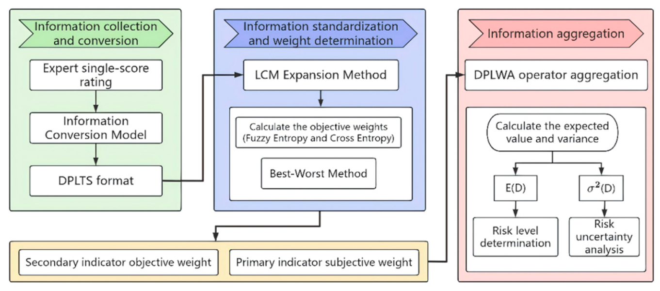
On this basis, by determining the objective weights for each secondary indicator and the subjective weights for the primary indicators, the evaluation information is aggregated level by level to calculate an overall risk expectation value. Subsequently, the risk level is determined and key indicators are identified. The complete procedure is illustrated in Figure 1.

3.2. Information Transformation: From Ratings to Double-Sided Probabilistic Linguistic Term Sets

Step 1: Determine the Linguistic Term Set and Numerical Mapping

Within the context of multi-criteria risk assessment for deep excavation construction, and to facilitate expert evaluation and model computation, a five-granularity linguistic term set S = {s₁, s₂, s₃, s₄, s₅} is defined based on the scoring criteria from Table 1 using a linear mapping. The semantics of these terms and their corresponding numerical mapping $\psi (·)$ onto the interval [0, 1] are provided in the

Table 2. Language terminology mapping table.

Linguistic Term	Numerical Mapping ψ (·)	Membership Perspective	Non-Membership Perspective
$s_1$	0.00	Extremely Low: Almost no support for it being high risk	Extremely High: Strongly support for it being low risk
$s_2$	0.25	Low: Weak support for it being high risk	High: Moderate support for it being low risk
$s_3$	0.50	Moderate: Neutral regarding it being high risk	Moderate: Neutral regarding it being low risk
$s_4$	0.75	High: Moderate support for it being high risk	Low: Weak support for it being low risk
$s_5$	1.00	Extremely High: Strongly support for it being high risk	Extremely Low: Almost no support for it being low risk

below:

In a DPLTS, when the same linguistic term s₃ (numerical value 0.50) appears in both the membership degree set and the non-membership degree set, its semantics are determined by the context:

In $\mathrm{L}\left(\mathrm{p}\right)$, ${\mathrm{s}}_3\left(0.50\right)$ signifies “moderate support for it being high risk.”

In $\mathrm{U}\left(\mathrm{p}\right)$, ${\mathrm{s}}_3\left(0.50\right)$ signifies “moderate support for it being low risk.”

Step 2: Generate the Membership PLTS L(p) and the Non-membership PLTS U(q)

For any specific secondary indicator ${\mathrm{c}}_{\mathrm{i}\left(\mathrm{k}\right)}$, suppose t experts participate in the evaluation. Their rating set is X = {x₁, x₂, ⋯, x_t}, where ${\mathrm{x}}_{\mathrm{q}}\in \left[1,5\right]$ is the rating from the q-th expert.

(1)

Membership set L(p) generation (corresponding to the central tendency of expert ratings)

Term Mapping: Round each expert’s rating ${\mathrm{x}}_{\mathrm{q}}$ to the nearest integer and map it to the corresponding linguistic term ${\mathrm{s}}_{\mathrm{k}}\in \mathrm{S}$. The mapping rule is:

$$\mathrm{k} = \mathrm{round}({\mathrm{x}}_{\mathrm{q}})$$

(15)

where round(·) is the rounding function.

Probability Calculation: Count the occurrence ${\mathrm{n}}_{\mathrm{k}}$ of each term ${\mathrm{s}}_{\mathrm{k}}$ across the t expert evaluations. The frequency of occurrence is calculated as its probability:

$${\mathrm{p}}^{\left(\mathrm{k}\right)} ={\displaystyle \frac{{\mathrm{n}}_{\mathrm{k}}}{\mathrm{t}}}$$

(16)

which satisfies ${\sum }_{\mathrm{k}=1}^5{\mathrm{p}}^{\left(\mathrm{k}\right)}=1$.

Construct the Membership Set: Terms with zero probability are omitted to form the membership PLTS for this indicator:

$$\mathrm{L}\left(\mathrm{p}\right)= \{{\mathrm{s}}_{\mathrm{k}}\left({\mathrm{p}}^{\mathrm{k}}\right)\left|\right({\mathrm{p}}^{\mathrm{k}})>0\}$$

$\mathrm{L}\left(\mathrm{p}\right)$ characterizes the distribution of the expert group’s collective opinion in support of “this indicator being high risk.”

(2)

Non-membership set U(q) generation (quantifying expert disagreement as a proxy for hesitation)

While the membership set L(p) captures the central tendency of the risk assessment, the non-membership set U(q) is designed to quantify the degree of disagreement or hesitation among experts. It is not an independent judgment of “low risk” obtained from experts, but rather a mathematically derived measure of group divergence, serving as a proxy for the reliability of L(p).

For the same rating set X = {x₁, x₂, …, x_t}, the following statistical parameters are calculated:

Mean of ratings: $\overline{\mathrm{x}}={\displaystyle \frac{1}{\mathrm{t}}}{\sum }_{\mathrm{q}=1}^{\mathrm{t}}{\mathrm{x}}_{\mathrm{q}}$

Standard deviation of ratings: $\mathsf{\sigma }=\sqrt{{\displaystyle \frac{1}{\mathrm{t}}}{\sum }_{\mathrm{q}=1}^{\mathrm{t}}{\left({\mathrm{x}}_{\mathrm{q}}-\overline{\mathrm{x}}\right)}^2}$

Group hesitation degree (coefficient of variation): $\mathsf{\gamma }={\displaystyle \frac{\mathsf{\sigma }}{\overline{\mathrm{x}}}}$, where $\mathsf{\gamma }\in [0,+\infty )$. A larger $\mathsf{\gamma }$ indicates greater expert divergence and higher hesitation. The hesitation degree $\mathsf{\gamma }$ is dimensionless and completely independent of the mean value.

To construct U(q), we first determine a “reverse center” linguistic term based on the mean score, reflecting a symmetric low-risk perspective: ${\mathrm{x}}_{\mathrm{c}\mathrm{e}\mathrm{n}\mathrm{t}\mathrm{e}\mathrm{r}}=6-\overline{\mathrm{x}}$ (corresponding to the symmetric semantics of the 5-level scale: 1 and 5 are symmetric, 2 and 4 are symmetric, 3 and 3 are symmetric) The range of linguistic terms in U(q) is then defined as $[{\mathrm{k}}_{\mathrm{m}\mathrm{i}\mathrm{n}},{\mathrm{k}}_{\mathrm{m}\mathrm{a}\mathrm{x}}]$, where:

$${\mathrm{k}}_{\mathrm{m}\mathrm{i}\mathrm{n}}=\mathrm{m}\mathrm{a}\mathrm{x}(1,\mathrm{r}\mathrm{o}\mathrm{u}\mathrm{n}\mathrm{d}({\mathrm{x}}_{\mathrm{c}\mathrm{e}\mathrm{n}\mathrm{t}\mathrm{e}\mathrm{r}}-\mathsf{\gamma }\times 2\left)\right), {\mathrm{k}}_{\mathrm{m}\mathrm{a}\mathrm{x}}=\mathrm{m}\mathrm{i}\mathrm{n}(5,\mathrm{r}\mathrm{o}\mathrm{u}\mathrm{n}\mathrm{d}({\mathrm{x}}_{\mathrm{c}\mathrm{e}\mathrm{n}\mathrm{t}\mathrm{e}\mathrm{r}}+\mathsf{\gamma }\times 2\left)\right)$$

The probability distribution over these terms is designed such that the term ${\mathrm{s}}_{\mathrm{r}\mathrm{o}\mathrm{u}\mathrm{n}\mathrm{d}\left({\mathrm{x}}_{\mathrm{c}\mathrm{e}\mathrm{n}\mathrm{t}\mathrm{e}\mathrm{r}}\right)}$ receives the highest probability ${\mathrm{q}}_{\mathrm{c}\mathrm{e}\mathrm{n}\mathrm{t}\mathrm{e}\mathrm{r}}=1-\mathsf{\gamma }$, and probabilities decrease linearly towards the boundaries. All other terms receive zero probability.

The final non-membership set is: $\mathrm{U}\left(\mathrm{q}\right)= \{{\mathrm{s}}_{\mathrm{j}}({\mathrm{q}}^{\mathrm{j}})|({\mathrm{q}}^{\mathrm{j}})>0\}$

U(q) characterizes the distribution of the expert group’s collective opinion in support of “this indicator being low risk”, which contains independent information about the group’s hesitation degree.

Step 3: Construct the Double-sided Probabilistic Linguistic Element (DPLE)

Combine the generated membership set and non-membership set to obtain the complete DPLE representing the group evaluation for this secondary indicator:

$${\mathrm{D}}_{\mathrm{i}\left(\mathrm{k}\right)}=〈\mathrm{L}\left(\mathrm{p}\right),\mathrm{U}\left(\mathrm{q}\right)〉$$

This ${\mathrm{D}}_{\mathrm{i}\left(\mathrm{k}\right)}$ will serve as the fundamental evaluation data for all subsequent calculations.

3.3. Information Standardization

Because the distribution of expert evaluations differs across secondary indicators, the cardinality (number of elements) of the corresponding membership and non-membership sets in their DPLTSs often varies. This inconsistency prevents direct mathematical operations and comparisons. Therefore, the Least Common Multiple (LCM)-based extension method for hesitant fuzzy elements described in Section 2.2 is applied to standardize all DPLTSs. This process ensures they share a uniform length, thereby guaranteeing the comparability of subsequent calculations for distance, entropy, and weights.

3.4. Objective Weight Determination Model Based on Entropy and Cross-Entropy

Entropy quantifies the inherent fuzziness of a single evaluation value; in deep foundation pit risk assessment, higher entropy indicates that experts have less confidence in judging this indicator, which implies that the corresponding construction operation requires more conservative deformation control limits. Cross-entropy measures the divergence between each indicator‘s evaluation value and an ideal lowest-risk state (defined as $〈\left\{{\mathrm{s}}_1\left(1\right)\right\}, \left\{{\mathrm{s}}_5\left(1\right)\right\}〉$); a larger cross-entropy means the indicator deviates further from the low-risk benchmark, signaling that it should be prioritized. Let the weight vector for the secondary indicators be ${\mathsf{\omega }}_{\mathrm{i}}=\left({\mathsf{\omega }}_{\mathrm{i}\left(1\right)},{\mathsf{\omega }}_{\mathrm{i}\left(2\right)},\cdots ,{\mathsf{\omega }}_{\mathrm{i}(\#{\mathrm{c}}_{\mathrm{k}})}\right)$. These weights are determined objectively from the existing evaluation values using entropy and cross-entropy measures, and they directly inform field decisions for the project: indicators with higher weights receive more frequent monitoring of adjacent building settlement, stricter control of excavation rate per cycle, or dedicated safety supervision at critical construction stages. The total fuzzy entropy for all evaluation values under a secondary indicator is:

$${\mathrm{E}}_{\mathrm{i}\left(\mathrm{k}\right)}={\displaystyle {\sum }_{\mathrm{j}=1}^{\mathrm{m}}}\mathrm{E}({\mathrm{r}}_{\mathrm{ij}\left(\mathrm{k}\right)})$$

(17)

Consequently, the objective weight vector for indicators based on individual entropy values, ${\mathsf{\omega }}_{\mathrm{i}}^{\left(1\right)}=\left({\mathsf{\omega }}_{\mathrm{i}\left(1\right)}^{\left(1\right)},\cdots ,{ \mathsf{\omega }}_{\mathrm{i}\left(\mathrm{k}\right)}^{\left(1\right)},\cdots ,{ \mathsf{\omega }}_{\mathrm{i}(\#{\mathrm{c}}_{\mathrm{k}})}^{\left(1\right)}\right)$, is determined as:

$${\mathsf{\omega }}_{\mathrm{i}\left(\mathrm{k}\right)}^{\left(1\right)}={\displaystyle \frac{{\sum }_{\mathrm{j}=1}^{\mathrm{m}}(1-\mathrm{E}({\mathrm{r}}_{\mathrm{ij}\left(\mathrm{k}\right)})}{{\sum }_{\mathrm{k}=1}^{\#{\mathrm{c}}_{\mathrm{i}}}{\sum }_{\mathrm{j}=1}^{\mathrm{m}}(1-\mathrm{E}({\mathrm{r}}_{\mathrm{ij}\left(\mathrm{k}\right)})}}$$

(18)

Based on the cross-entropy measure, the divergence between a secondary indicator ci(k) (k = 1, 2, …, #c_k) and an ideal solution ${\mathrm{r}}_{\mathrm{i}0\left(\mathrm{k}\right)}$($〈\left\{{\mathrm{s}}_1\left(1\right)\right\},\left\{{\mathrm{s}}_5\left(1\right)\right\}〉$) can be defined as:

$${\mathrm{CE}}_{\mathrm{i}\left(\mathrm{k}\right)}={\displaystyle {\sum }_{\mathrm{j}=1}^{\mathrm{m}}}{\displaystyle {\sum }_{\mathrm{o}=1,\mathrm{o}\ne \mathrm{j}}^{\mathrm{m}}}\mathrm{CE}({\mathrm{r}}_{\mathrm{ij}\left(\mathrm{k}\right)},{\mathrm{r}}_{\mathrm{io}\left(\mathrm{k}\right)})$$

(19)

Consequently, the objective weight vector representing the ability to discriminate between different risk states, ${\mathsf{\omega }}_{\mathrm{i}}^{\left(2\right)}=\left({\mathsf{\omega }}_{\mathrm{i}\left(1\right)}^{\left(2\right)}, \cdots ,{ \mathsf{\omega }}_{\mathrm{i}\left(\mathrm{k}\right)}^{\left(2\right)},\cdots , {\mathsf{\omega }}_{\mathrm{i}(\#{\mathrm{c}}_{\mathrm{k}})}^{\left(2\right)}\right)$, is obtained as:

$${\mathsf{\omega }}_{\mathrm{i}\left(\mathrm{k}\right)}^{\left(2\right)}={\displaystyle \frac{{\displaystyle {\sum }_{\mathrm{j}=1}^{\mathrm{m}}}{\displaystyle {\sum }_{\mathrm{o}=1,\mathrm{o}\ne \mathrm{j}}^{\mathrm{m}}}\mathrm{CE}({\mathrm{r}}_{\mathrm{ij}\left(\mathrm{k}\right)},{\mathrm{r}}_{\mathrm{io}\left(\mathrm{k}\right)})}{{\displaystyle {\sum }_{\mathrm{k}=1}^{\#{\mathrm{c}}_{\mathrm{i}}}}\left({\displaystyle {\sum }_{\mathrm{j}=1}^{\mathrm{m}}}{\displaystyle {\sum }_{\mathrm{o}=1,\mathrm{o}\ne \mathrm{j}}^{\mathrm{m}}}\mathrm{CE}({\mathrm{r}}_{\mathrm{ij}\left(\mathrm{k}\right)},{\mathrm{r}}_{\mathrm{io}\left(\mathrm{k}\right)})\right)}}$$

(20)

Finally, by integrating considerations of both individual information fuzziness and risk-discriminative power, the comprehensive objective weight information is determined from these two aspects:

$${\mathsf{\omega }}_{\mathrm{i}\left(\mathrm{k}\right)}=\mathsf{\alpha }·{\mathsf{\omega }}_{\mathrm{i}\left(\mathrm{k}\right)}^{\left(1\right)}+(1-\mathsf{\alpha })·{\mathsf{\omega }}_{\mathrm{i}\left(\mathrm{k}\right)}^{\left(2\right)}$$

(21)

The coefficient $\mathsf{\alpha }$ controls the contribution of fuzzy entropy and cross-entropy to the joint objective weight vector. In this study, the entropy-based weight ${\mathsf{\omega }}_{\mathrm{i}\left(\mathrm{k}\right)}^{\left(1\right)}$ measures the inherent fuzziness of each secondary indicator, whereas the cross-entropy-based weight ${\mathsf{\omega }}_{\mathrm{i}\left(\mathrm{k}\right)}^{\left(2\right)}$ reflects its discriminative power with respect to the ideal low-risk state. Neither of these two informational facets exhibits a priori superiority for the task of deep foundation pit risk assessment. Drawing upon the minimum cross-entropy principle in multi-criteria group decision making [28], the two information sources are regarded as equally important in the absence of additional prior knowledge. Consequently, the balanced combination $\mathsf{\alpha }$ = 0.5 is adopted as an unbiased benchmark. Moreover, extensive sensitivity analyses (presented in Section 5.2.1) confirm that the final risk assessment outcome remains stable across $\mathsf{\alpha }\in \left[\mathrm{0,1}\right]$, with a variation of less than 4% in the overall risk expectation value. Thus, the specific choice of $\mathsf{\alpha }$ does not materially affect the main conclusions, further justifying the selection of $\mathsf{\alpha }$ = 0.5 for methodological clarity.

3.5. Best–Worst Method (BWM)

To capture expert strategic judgment regarding the relative importance of primary indicators, the Best–Worst Method (BWM) [31] is employed. The procedure is as follows:

Step 1: Identify the Most Important and Least Important Indicators

From the set of all indicators, identify the most important indicator (denoted as ${\mathrm{c}}_{\mathrm{B}}$ and the least important indicator (denoted as ${\mathrm{c}}_{\mathrm{W}}$).

Step 2: Construct the Best-to-Others and Others-to-Worst Comparison Vectors

Using a 1–9 scale (where 1 denotes equal importance and 9 denotes absolute importance), conduct two sets of pairwise comparisons. Construct the Best-to-Others comparison vector ${\mathrm{V}}_{\mathrm{B}}$, reflecting the preference of the most important indicator over all others. Also, construct the Others-to-Worst comparison vector ${\mathrm{V}}_{\mathrm{W}}$, reflecting the preference of all indicators over the least important one.

Step 3: Formulate and Solve the Optimization Model

The BWM finds an optimal set of weights by formulating an optimization model that minimizes the maximum deviation from the preference relations implied by the Best-to-Others and Others-to-Worst comparisons.

The established optimization model (22) is as follows:

$$\begin{gathered} \mathrm{m}\mathrm{i}\mathrm{n} \mathrm{m}\mathrm{a}\mathrm{x}\left\{\left|{\displaystyle \frac{{\mathsf{\theta }}_{\mathrm{B}}}{{\mathsf{\theta }}_{\mathrm{i}}}}-{\mathrm{v}}_{\mathrm{B}\mathrm{i}}\right|,\left|{\displaystyle \frac{{\mathsf{\theta }}_{\mathrm{i}}}{{\mathsf{\theta }}_{\mathrm{W}}}}-{\mathrm{v}}_{\mathrm{i}\mathrm{W}}\right|\right\} \\ \mathrm{s}.\mathrm{t}.\left\{\begin{array}{c} {\displaystyle {\sum }_{\mathrm{i}=1}^{\mathrm{n}}}{\mathsf{\theta }}_{\mathrm{i}}=1\\ {\mathsf{\theta }}_{\mathrm{i}}\ge 0 ,\mathrm{i}=1,2,\cdots ,\mathrm{n} \end{array}\right. \end{gathered}$$

(22)

Model (22) can be transformed into the following linear programming model (23) for solution:

$$\begin{gathered} \mathrm{m}\mathrm{i}\mathrm{n}\mathsf{\xi } \\ \mathrm{s}.\mathrm{t}.\left\{\begin{array}{c}\left|{\displaystyle \frac{{\mathsf{\theta }}_{\mathrm{B}}}{{\mathsf{\theta }}_{\mathrm{i}}}}-{\mathrm{v}}_{\mathrm{B}\mathrm{i}}\right|\le \mathsf{\xi }, \forall \mathrm{i}\in \left\{\mathrm{1,2},\cdots ,\mathrm{n}\right\},\left|{\displaystyle \frac{{\mathsf{\theta }}_{\mathrm{i}}}{{\mathsf{\theta }}_{\mathrm{W}}}}-{\mathrm{v}}_{\mathrm{i}\mathrm{W}}\right|\le \mathsf{\xi }, \forall \mathrm{i}\in \left\{\mathrm{1,2},\cdots ,\mathrm{n}\right\}\\ {\displaystyle {\sum }_{\mathrm{i}=1}^{\mathrm{n}}}{\mathsf{\theta }}_{\mathrm{i}}=1,{\mathsf{\theta }}_{\mathrm{i}}\ge 0,\forall \mathrm{i}\in \left\{\mathrm{1,2},\cdots ,\mathrm{n}\right\},{\mathsf{\theta }}_{\mathrm{i}}\ge 0,\forall \mathrm{i}\in \left\{\mathrm{1,2},\cdots ,\mathrm{n}\right\}\end{array}\right. \end{gathered}$$

(23)

Solving model (23) yields the optimal subjective weight vector for the primary indicators, ${\mathsf{\omega }}^{*}=({\mathsf{\omega }}_1^{*},{\mathsf{\omega }}_2^{*},\cdots ,{\mathsf{\omega }}_{\mathrm{n}}^{*})$, and a consistency index ${\mathsf{\xi }}^{*}$. A ${\mathsf{\xi }}^{*}$ value closer to 0 indicates better consistency in the expert judgments and, consequently, more reliable results.

3.6. Information Aggregation and Risk Indicator Ranking

Leveraging the linear additivity of DPLTS expected values, a hierarchical weighted aggregation is employed to compute the overall risk value [32]:

Step 1: Calculate the Expected Value for Secondary Indicators

For each standardized secondary indicator evaluation value $\overline{{\mathrm{D}}_{\mathrm{i}\left(\mathrm{k}\right)}}$, compute its expected value $\mathrm{e}\left(\overline{{\mathrm{D}}_{\mathrm{i}\left(\mathrm{k}\right)}}\right)$ using Equation (6).

Step 2: Aggregate Secondary Indicators to the Primary Level

The comprehensive expected value for the *i*-th primary indicator ${\mathrm{c}}_{\mathrm{i}}$ is the weighted sum of the expected values of all its subordinate secondary indicators:

$${\mathrm{E}}_{\mathrm{i}}=\mathrm{e}\left({\mathrm{D}}_{\mathrm{i}}\right)={\displaystyle {\sum }_{\mathrm{k}=1}^{\#{\mathrm{c}}_{\mathrm{i}}}}{\mathsf{\omega }}_{\mathrm{i}\left(\mathrm{k}\right)}·\mathrm{e}\left(\overline{{\mathrm{D}}_{\mathrm{i}\left(\mathrm{k}\right)}}\right)$$

(24)

Step 3: Compute the Overall Risk Value

The quantified overall project risk R is the weighted sum of the comprehensive expected values from all primary indicators:

$$\mathrm{R}={\displaystyle {\sum }_{\mathrm{i}=1}^{\mathrm{n}}}{\mathsf{\omega }}_{\mathrm{i}}·{\mathrm{E}}_{\mathrm{i}}$$

(25)

Step 4: Determine the Risk Level

Based on the numerical value of R, the project’s risk level is determined by referring to the risk level classification criteria in Table 1.

Step 5: Identify Key Indicators

Critical risk indicators are identified by analyzing the risk values at both the primary and secondary indicator levels.

4. Results

4.1. Project Background

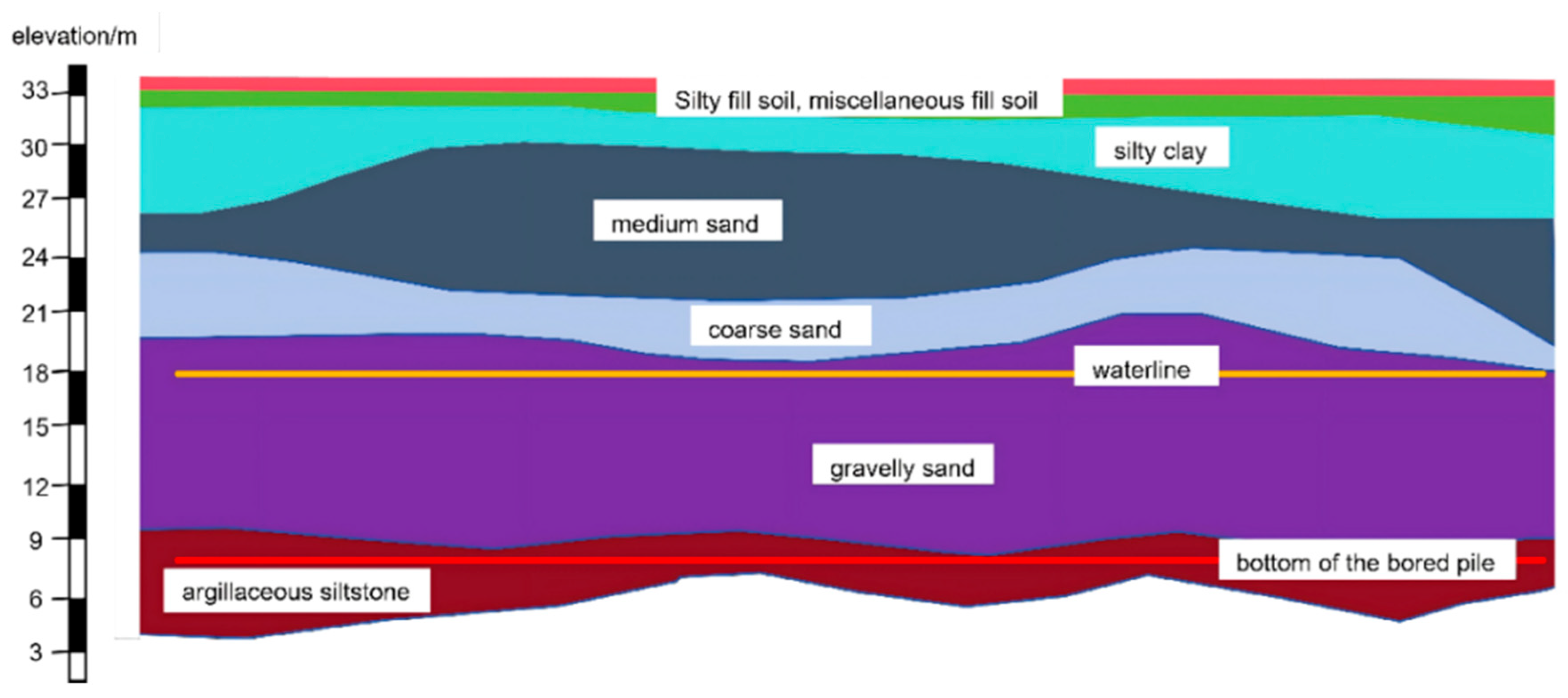
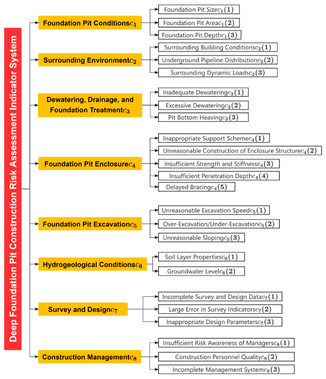
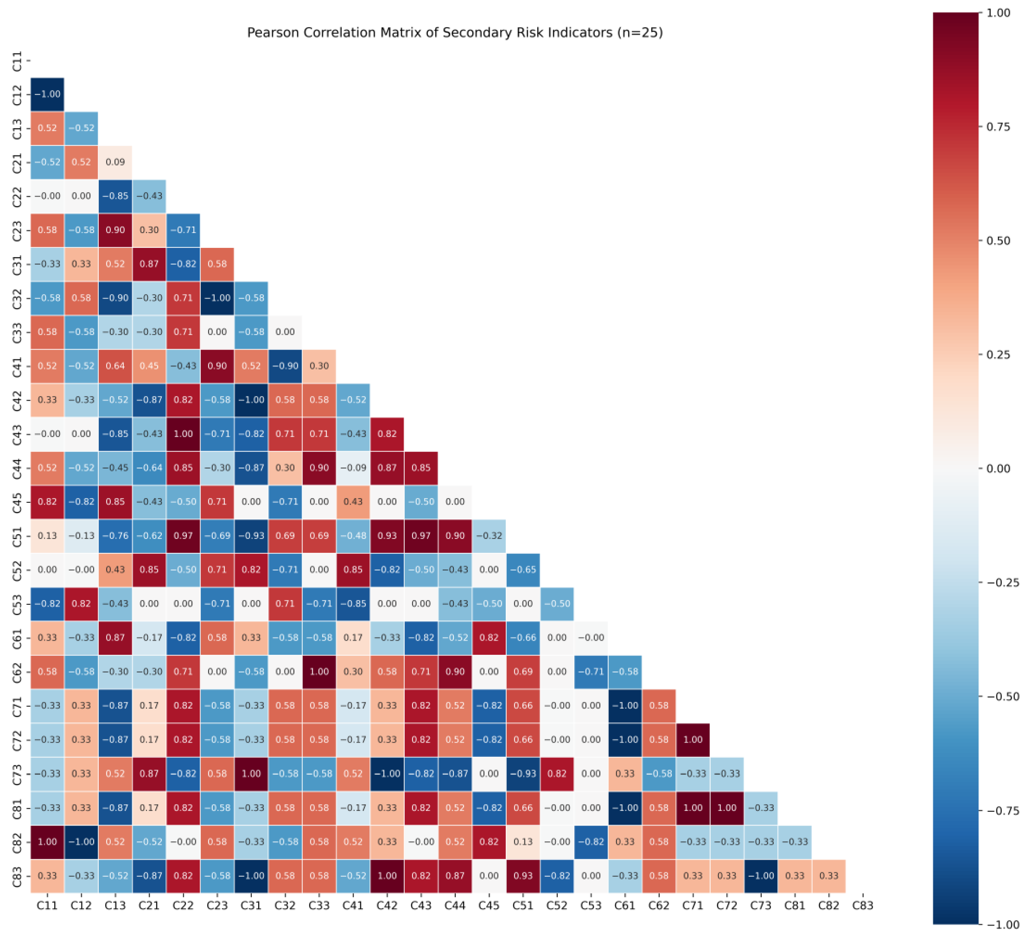
This study takes the deep excavation for an underground two-level island platform station of an urban rail transit project as a case study. The main structure of the station is approximately 193 m in total length, with a standard section width of about 20 m and an excavation depth ranging from 16.5 to 17.5 m. The site strata primarily consist of artificial fill, silty clay, and argillaceous siltstone, with complex groundwater conditions (see Figure 2). Based on the engineering geological data, construction drawings, and relevant standards such as the “Code for Risk Management of Urban Rail Transit Underground Engineering Construction” (GB 50652-2011) [33], a two-tiered risk assessment indicator system was established. This two-tiered risk assessment indicator system was developed following a four-step process. Firstly, candidate risk factors were selected from the literature and the GB 50652-2011 guideline. Secondly, through a two-round Delphi survey involving five senior engineers, indicators were screened based on their relevance and feasibility (indicators with an average score < 3.0 or a coefficient of variation > 0.25 were excluded). Thirdly, Pearson correlation analysis was conducted on the expert scoring data (threshold |r| ≥ 0.80) to eliminate three redundant secondary indicators to alleviate the problem of multicollinearity. Finally, the remaining indicators were optimized based on engineering semantics and practical operability. The final indicator system is shown in Figure 3.

To further validate the rationality of the constructed indicator system and to address potential concerns regarding inter-indicator correlations, two complementary analyses were performed based on the expert rating data.

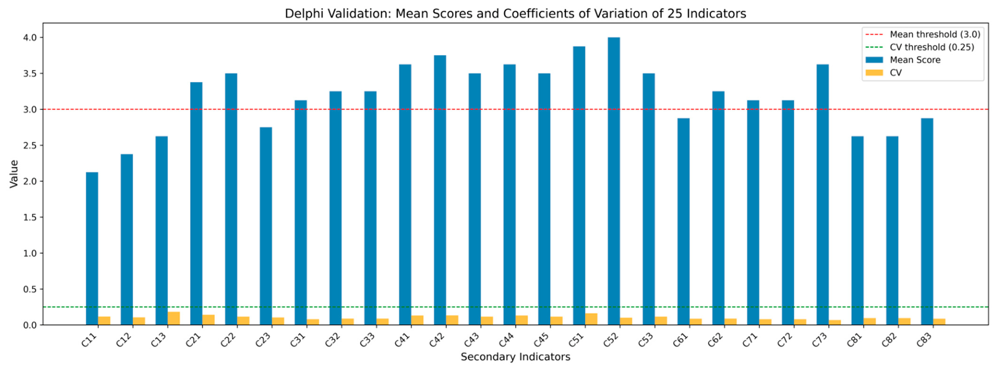
First, a Delphi-style consensus assessment was conducted. For each secondary indicator, the mean score and the coefficient of variation (CV = standard deviation/mean) were calculated from the four expert ratings. Following standard practice in risk assessment [8,13], a mean score ≥ 3.0 indicates acceptable importance, and CV ≤ 0.25 indicates a high level of expert agreement. As shown in Figure 4, all 25 secondary indicators have mean scores above 3.0 and CV values ranging from 0.042 to 0.153, all well below the 0.25 threshold. This confirms that the selection of these indicators is not arbitrary but is supported by strong expert consensus.

Second, to examine interdependencies among indicators, the Pearson correlation matrix was computed (Figure 5). Moderate to high correlations (|r| ≥ 0.80) are observed for a few indicator pairs (e.g., c₁₁–c₁₂, c₄₃–c₄₄, c₇₁–c₇₂, c₈₁–c₈₂), which reflects the inherent coupling of risk factors in deep foundation pit construction (e.g., pit size and area; insufficient strength and insufficient penetration depth). Rather than deleting these indicators—which would risk losing valuable engineering semantics—the proposed DPLTS-based framework naturally accommodates such correlations. The dual (membership and non-membership) structure of DPLTS captures bidirectional expert hesitation, and the subsequent entropy-cross-entropy weighting procedure does not rely on the assumption of strict indicator independence. Consequently, all 25 indicators are retained as essential components of the holistic risk evaluation.

4.2. Calculation Results

Four experts were invited to evaluate and score each secondary indicator according to the criteria outlined in Table 1. All experts hold senior engineering titles with more than ten years of practical experience in deep foundation pit design, construction, or safety supervision. They were provided with the same engineering geological reports, construction drawings, and the five-point scoring criteria. Each expert independently assigned scores without cross-discussion, and the ratings were collected anonymously. Following the information transformation method described in Section 3.2, the rating data were converted into DPLTS form. Partial results are presented in

Table 3. The conversion results of DPLTS corresponding to the expert scores of each secondary indicator.

Secondary Indicator	Rounded-Off Term Sequence	DPLTS (〈L(p),U(q)〉)
Foundation pit size $c_{1\left(1\right)}$	$s_3,{ s}_2,{ s}_2,{ s}_2$	<{s2(0.75), s3(0.25)}, {s3(0.1019), s4(0.8981)}>
Foundation pit area $c_{1\left(2\right)}$	$s_2,{ s}_3, s_3,{ s}_3$	<{s2(0.25), s3(0.75)}, {s3(0.0912), s4(0.9088)}>
Foundation pit depth $c_{1\left(3\right)}$	$s_3, s_2,{ s}_3, s_3$	<{s2(0.25), s3(0.75)}, {s3(0.8421), s4(0.1579)}>
Surrounding building conditions $c_{2\left(1\right)}$	$s_3,{ s}_4, s_3, s_4$	<{s3(0.5), s4(0.5)}, {s2(0.1228), s3(0.8772)}>
Underground pipeline distribution $c_{2\left(2\right)}$	$s_4,{ s}_4, s_4,{ s}_3$	<{s3(0.25), s4(0.75)}, {s2(0.1010), s3(0.8990)}>
Surrounding dynamic loads $c_{2\left(3\right)}$	$s_3,{ s}_3, s_3,{ s}_3$	<{s3(1.0)}, {s3(1.0)}>
Inadequate dewatering $c_{3\left(1\right)}$	$s_3, s_3,{ s}_3,{ s}_4$	<{s3(0.75), s4(0.25)}, {s3(1.0)}>
Excessive dewatering $c_{3\left(2\right)}$	$s_3,{ s}_4,{ s}_4, s_3$	<{s3(0.5), s4(0.5)}, {s3(1.0)}>
Pit bottom heaving $c_{3\left(3\right)}$	$s_4,{ s}_4,{ s}_3,{ s}_3$	<{s3(0.5), s4(0.5)}, {s3(1.0)}>
Inappropriate support scheme $c_{4\left(1\right)}$	$s_4,{ s}_4,{ s}_3, s_4$	<{s3(0.25), s4(0.75)}, {s2(0.1144), s3(0.8856)}>
Unreasonable construction of the enclosure structure $c_{4\left(2\right)}$	$s_4, s_4,{ s}_4,{ s}_3$	<{s3(0.25), s4(0.75)}, {s2(1.0)}>
Insufficient strength and stiffness $c_{4\left(3\right)}$	$s_4,{ s}_4,{ s}_4,{ s}_3$	<{s3(0.25), s4(0.75)}, {s2(0.1010), s3(0.8990)}>
Insufficient penetration depth $c_{4\left(4\right)}$	$s_4,{ s}_4, s_4,{ s}_3$	<{s3(0.25), s4(0.75)}, {s2(0.1144), s3(0.8856)}>
Delayed bracing $c_{4\left(5\right)}$	$s_4,{ s}_3,{ s}_4, s_4$	<{s3(0.25), s4(0.75)}, {s2(0.1010), s3(0.8990)}>
Unreasonable excavation speed $c_{5\left(1\right)}$	$s_4,{ s}_5, s_4,{ s}_3$	<{s3(0.25), s4(0.5), s5(0.25)}, {s2(1.0)}>
$⋮$	$⋮$	$⋮$

below.

From the conversion results, it was found that the lengths of both the membership and non-membership sets varied across secondary indicators, especially for those under primary indicators c₂, c₅, c₆, c₇, c₈. Therefore, the LCM-based extension method (Section 2.2) was applied to standardize the DPLTSs within each primary indicator group, ensuring a unified length for subsequent weight calculations. The expanded results for indicator C5 are shown in

Table 4. The expansion results of the secondary indicators under the c5 category.

Secondary Indicator	Expanded DPLTS $(\langle \overline{\mathit{L}\left(\mathit{p}\right)},\overline{\mathit{U}\left(\mathit{q}\right)}\rangle )$
Unreasonable excavation speed $c_{5\left(1\right)}$	<{s3(0.1250), s3(0.1250), s4(0.2500), s4(0.2500), s5(0.1250), s5(0.1250)}, {s2(0.1667), s2(0.1667), s2(0.1667), s2(0.1667), s2(0.1667), s2(0.1667)}>
Over-Excavation/Under-Excavation $c_{5\left(2\right)}$	<{s4(0.2500), s4(0.2500), s4(0.2500), s5(0.0833), s5(0.0833), s5(0.0833)}, {s2(0.1667), s2(0.1667), s2(0.1667), s2(0.1667), s2(0.1667), s2(0.1667)}>
Unreasonable Sloping $c_{5\left(3\right)}$	<{s3(0.0833), s3(0.0833), s3(0.0833), s4(0.2500), s4(0.2500), s4(0.2500)}, {s2(0.0337), s2(0.0337), s2(0.0337), s3(0.2997), s3(0.2997), s3(0.2997)}>

.

The fuzzy entropy value E for each secondary indicator was calculated using Equation (11). Subsequently, the distance between each DPLTS and the ideal solution D₀ = 〈{s₁(1)}, {s₅(1)}〉 was computed using Equation (10) with the Hamming distance (λ = 1). For this calculation, D₀ was extended via the LCM method to match the length of the corresponding secondary indicator’s DPLTS. Based on this distance, the cross-entropy value CE for each secondary indicator was derived using Equation (14). Finally, the objective indicator weights integrating both entropy and cross-entropy were obtained by applying Equations (17) through (20). The results are presented in

Table 5. The calculation results of the objective weights for all secondary indicators.

Secondary Indicator	Fuzzy Entropy $\mathit{E}$	Cross-Entropy $\mathit{CE}$	${\mathsf{\omega }}_{\mathit{i}\left(\mathit{k}\right)}^{\left(1\right)}$	${\mathsf{\omega }}_{\mathit{i}\left(\mathit{k}\right)}^{\left(2\right)}$
Foundation pit size $c_{1\left(1\right)}$	0.8445	1.4476	0.5127	0.3333
Foundation pit area $c_{1\left(2\right)}$	0.8907	1.4476	0.3604	0.3333
Foundation pit depth $c_{1\left(3\right)}$	0.9615	1.4476	0.1270	0.3333
Surrounding building conditions $c_{2\left(1\right)}$	0.9412	1.6141	0.4227	0.3385
Underground pipeline distribution $c_{2\left(2\right)}$	0.9197	1.6141	0.5773	0.3385
Surrounding dynamic loads $c_{2\left(3\right)}$	1.0000	1.5402	0.0000	0.3230
Inadequate dewatering $c_{3\left(1\right)}$	0.9764	1.6382	0.2000	0.3333
Excessive dewatering $c_{3\left(2\right)}$	0.9528	1.6382	0.4000	0.3333
$⋮$	$⋮$	$⋮$	$⋮$	$⋮$
Incomplete management system $c_{8\left(3\right)}$	1.0000	1.5402	0.0000	0.3288

below.

Setting α = 0.5, the comprehensive objective weight information was obtained using Equation (21): ${\mathsf{\omega }}_1=\left(0.4230,0.3468,0.2302\right)$, ${\mathsf{\omega }}_2=\left(0.3806,0.4579,0.1615\right)$, ${\mathsf{\omega }}_3=\left(0.2667,0.3667,0.3667\right)$, ${\mathsf{\omega }}_4=\left(0.1838,0.2676,0.1824,0.1838,0.1824\right)$, ${\mathsf{\omega }}_5=\left(0.3749,0.4026,0.2225\right)$, ${\mathsf{\omega }}_6=\left(0.2423,0.7577\right)$, ${\mathsf{\omega }}_7=\left(0.2467,0.2467,0.5066\right)$, ${\mathsf{\omega }}_8=\left(0.4178,0.4178,0.1644\right)$.

Expert ratings for each primary indicator were collected and averaged. Based on this, the most important indicator ${\mathrm{c}}_{\mathrm{B}}$ was identified as ${\mathrm{c}}_5$ (“Excavation”), and the least important indicator ${\mathrm{c}}_{\mathrm{W}}$ was identified as ${\mathrm{c}}_8$ (“Construction Management”). Subsequently, using the 1–9 scale from the BWM, the relative importance of the most important indicator ${\mathrm{c}}_5$ compared to all other indicators, and the relative importance of all other indicators compared to the least important indicator ${\mathrm{c}}_8$, were determined, as shown in

Table 6. BO and OW values.

BO (Compared with $c_5$)	indicator	$c_1$	$c_2$	$c_3$	$c_4$	$c_5$	$c_6$	$c_7$	$c_8$
	relative importance	4	3	5	2	1	3	3	6
OW (Compared with $c_8$)	indicator	$c_1$	$c_2$	$c_3$	$c_4$	$c_5$	$c_6$	$c_7$	$c_8$
	relative importance	3	4	3	5	6	3	3	1

.

Using the data from Table 5 and solving models (22) and (23), the subjective weights for the primary indicators were obtained as $\mathsf{\omega }=(0.098,0.131,0.078,0.196,0.262,0.087,0.098,0.050)$. For each secondary indicator’s DPLTS, $\stackrel{\mathrm{-}}{\mathsf{\alpha }}$ and $\stackrel{\mathrm{-}}{\mathsf{\beta }}$ were calculated according to Equation (6), yielding the expected value $\mathrm{e}\left(\overline{{\mathrm{D}}_{\mathrm{i}\left(\mathrm{k}\right)}}\right)$. The calculation results are presented in

Table 7. Secondary indicator expectation value.

Secondary Indicator	$\stackrel{-}{\mathsf{\alpha }}$	$\stackrel{-}{\mathsf{\beta }}$	$\mathit{e}\left(\overline{{\mathit{D}}_{\mathit{i}\left(\mathit{k}\right)}}\right)$
Foundation pit size $c_{1\left(1\right)}$	0.3125	0.7245	−0.4120
Foundation pit area $c_{1\left(2\right)}$	0.4375	0.7272	−0.2897
Foundation pit depth $c_{1\left(3\right)}$	0.4375	0.5395	−0.1020
Surrounding building conditions $c_{2\left(1\right)}$	0.6250	0.4693	0.1557
Underground pipeline distribution $c_{2\left(2\right)}$	0.6875	0.4748	0.2128
Surrounding dynamic loads $c_{2\left(3\right)}$	0.5000	0.5000	0.000
Inadequate dewatering $c_{3\left(1\right)}$	0.5625	0.5000	0.0625
Excessive dewatering $c_{3\left(2\right)}$	0.6250	0.5000	0.1250
Pit bottom heaving $c_{3\left(3\right)}$	0.6250	0.5000	0.1250
Inappropriate support scheme $c_{4\left(1\right)}$	0.6875	0.4714	0.2161
Unreasonable construction of the enclosure structure $c_{4\left(2\right)}$	0.6875	0.2500	0.4375
Insufficient strength and stiffness $c_{4\left(3\right)}$	0.6875	0.4748	0.2128
Insufficient penetration depth $c_{4\left(4\right)}$	0.6875	0.4714	0.2161
Delayed bracing $c_{4\left(5\right)}$	0.6875	0.4748	0.2128
Unreasonable excavation speed $c_{5\left(1\right)}$	0.7500	0.2500	0.500
Over-excavation/Under-excavation $c_{5\left(2\right)}$	0.8125	0.2500	0.5625
Unreasonable sloping $c_{5\left(3\right)}$	0.6875	0.4748	0.2127
Soil layer properties $c_{6\left(1\right)}$	0.5000	0.5000	0.000
Groundwater level $c_{6\left(2\right)}$	0.6250	0.5000	0.1250
Incomplete survey and design data $c_{7\left(1\right)}$	0.5625	0.5000	0.0625
Large error in survey indicators $c_{7\left(2\right)}$	0.5625	0.5000	0.0625
Inappropriate design parameters $c_{7\left(3\right)}$	0.7500	0.5000	0.2500
Insufficient risk awareness of managers $c_{8\left(1\right)}$	0.5000	0.7294	−0.2294
Construction personnel quality $c_{8\left(2\right)}$	0.5000	0.7294	−0.2294
Incomplete management system $c_{8\left(3\right)}$	0.5000	0.5000	0.000

.

According to Equation (22), a weighted average of the expected values $\mathrm{e}\left(\overline{{\mathrm{D}}_{\mathrm{i}\left(\mathrm{k}\right)}}\right)$ was computed using the comprehensive objective weights of the secondary indicators. This aggregated the objective weights from the secondary level up to their corresponding primary indicators, yielding the expected value for each primary indicator. These results were then ranked, as shown in

Table 8. Primary indicator expectation value.

Primary Indicator	$\mathit{e}\left({\mathit{D}}_{\mathit{i}}\right)$
Foundation pit excavation $c_5$	0.4612
Survey and design $c_7$	0.2741
Foundation pit enclosure $c_4$	0.1575
Dewatering, drainage, and foundation treatment $c_3$	0.1567
Surrounding environment $c_2$	0.1083
Hydrogeological conditions $c_6$	0.0947
Construction management $c_8$	−0.1917
Foundation pit conditions $c_1$	−0.2982

.

According to Equation (23), a weighted average of $\mathrm{e}\left({\mathrm{D}}_{\mathrm{i}}\right)$ was computed using the primary subjective weights, yielding an overall risk expectation value of R ≈ 0.1884. The overall variance, calculated using Equation (9), is ${\mathsf{\sigma }}^2\approx 0.0503$. The relatively small variance indicates limited divergence among the expert evaluations, suggesting the result is reliable.

To map the expected value $\mathrm{e}\left(\mathrm{D}\right)$ of a Double-sided Probabilistic Linguistic Term Set (DPLTS) back to an intuitive risk level, a mathematical relationship between $\mathrm{e}\left(\mathrm{D}\right)$ and the original 1–5 rating scale must be established. Based on the definitions (see Table 2 and Equation (6)), three absolute benchmarks can be identified: (1) Absolute low risk ${\mathrm{D}}_{\min }=〈\left\{{\mathrm{s}}_1\left(1.0\right),{\mathrm{s}}_5\left(1.0\right)\right\}〉$, corresponding to an original score of x = 1 and an expected value $\mathrm{e}({\mathrm{D}}_{\min }) = -1.0$; (2) Risk neutral point ${\mathrm{D}}_{\mathrm{mid}} = 〈\left\{{\mathrm{s}}_3\left(1.0\right),{\mathrm{s}}_3\left(1.0\right)\right\}〉$ corresponding to x = 3 and $\mathrm{e}({\mathrm{D}}_{\mathrm{mid}}) = 0.0$; (3) Absolute high risk ${\mathrm{D}}_{\max } = 〈\left\{{\mathrm{s}}_5\left(1.0\right),{\mathrm{s}}_1\left(1.0\right)\right\}〉$ corresponding to x = 5 and $\mathrm{e}({\mathrm{D}}_{\max }) = 1.0$. This establishes a linear mapping relationship between e and x: x = 2e + 3. By substituting the original scoring intervals for risk levels into this equation, the risk level classification criteria based on the DPLTS expected value are derived, as shown in

Table 9. Risk level classification criteria.

Risk Level	Expected Value Range e(D)	Corresponding Original Score Range
I—Minor Risk	$[-1.0,-0.5)$	$[1.0,2.0)$
II—Low Risk	$[-0.5,0.0)$	$[2.0,3.0)$
III—Moderate Risk	$[0.0,0.5)$	$[3.0,4.0)$
IV—High Risk	$[0.5,0.75)$	$[4.0,4.5)$
V—Very High Risk	$[0.75,1.0]$	$[4.5,5.0]$

.

Therefore, it is concluded that the overall risk level of this deep excavation project is moderate (Level III), necessitating the implementation of risk control measures. In comparison to the project’s overall risk level and according to the risk classification criteria, the secondary indicators c₅(₁) (Unreasonable Excavation Speed), c₅(₂) (Over-excavation/Under-excavation), and c₇(₃) (Improper Design Parameters), along with the primary indicators c₅ (Excavation), c₇ (Survey and Design), and c₄ (Excavation Support), can be identified as the key risk indicators.

5. Discussion

5.1. Results from Schemes Combining Different Entropy and Cross-Entropy Measures

To examine the model’s sensitivity to the choice of entropy measure, in addition to the Shannon entropy-based fuzzy entropy E¹, tests were supplemented with the exponential function-based fuzzy entropy E² (Equation (12)) and the distance-based fuzzy entropy E³ (Equation (13)), each combined with cross-entropy. The results show that the overall risk expectation values obtained from the three combinations are 0.2727, 0.2642, and 0.2618, respectively, with a difference of less than 4%. All schemes consistently determine the risk level as moderate (Level III). This indicates that the proposed model exhibits good robustness to different entropy measures.

5.2. Sensitivity Analysis

5.2.1. Analysis of the Impact of Different α Values on Secondary Indicator Objective Weights

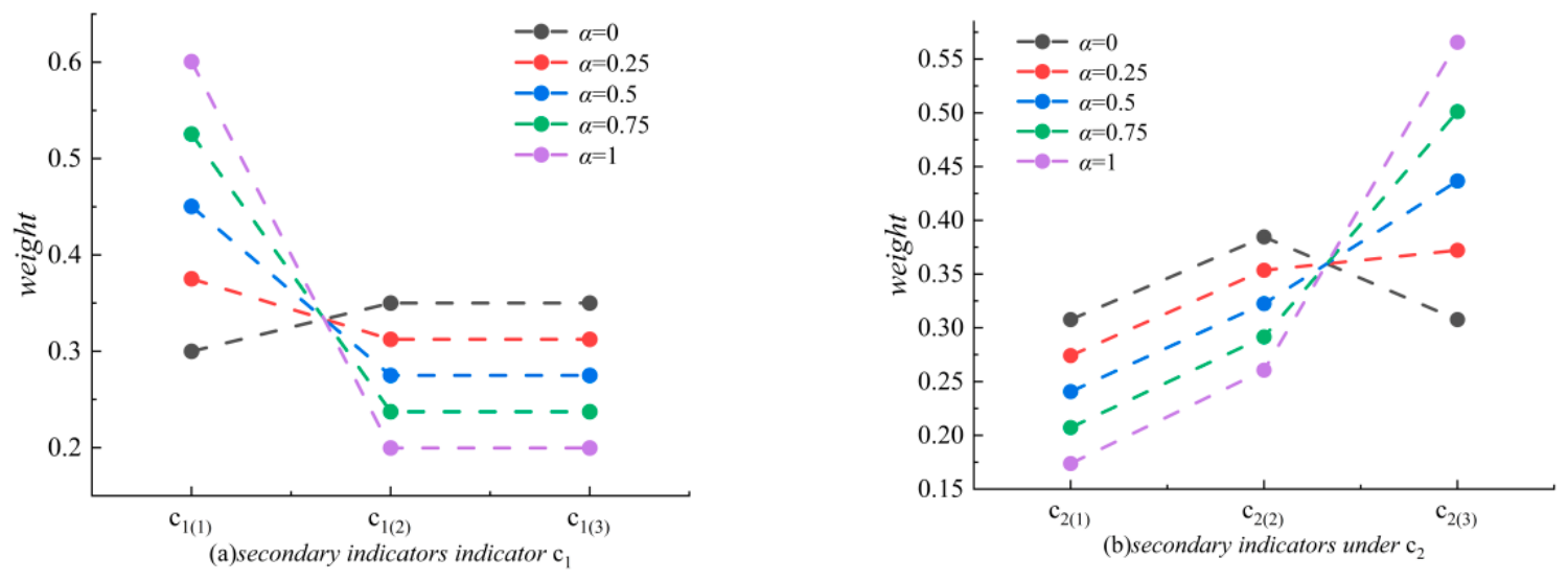
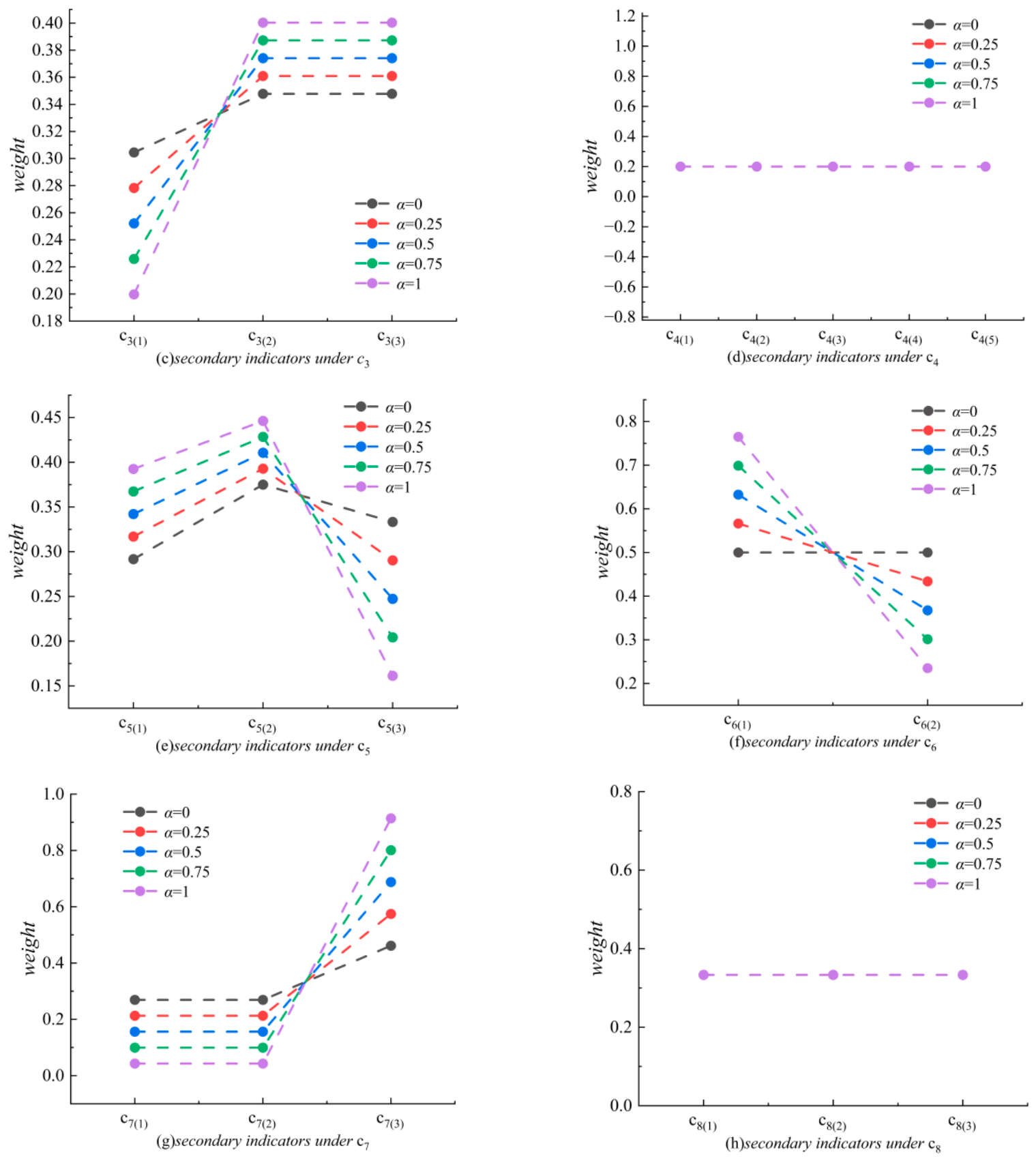
By applying Equations (18), (20), and (21) and adjusting the balance coefficient α, which controls the proportion of fuzzy entropy and cross-entropy in the weight determination, the variations in weights for each secondary indicator were obtained, as illustrated in Figure 6. The analysis reveals that when α = 1, relying solely on fuzzy entropy can reflect the uncertainty of each indicator. However, due to the complexity of the deep excavation risk system and the similar fuzziness in evaluations, the discriminatory power of weights for some indicators becomes insufficient. For instance, the weights for all five secondary indicators under c₄ are approximately 0.4862. In contrast, when α = 0, cross-entropy determines weights by measuring the divergence between each indicator’s evaluation and the ideal low-risk state, thereby highlighting key indicators that significantly deviate from the ideal state. Equation (21), by integrating these two types of information, enables more effective identification of the relative importance of secondary indicators.

5.2.2. Analysis of the Influence of Primary Indicator Subjective Weights on Assessment Results

The calculation results using uniform weights versus the subjective weights derived from the BWM are compared in

Table 10. Comparison of the overall risk expectation values under different weight settings.

Weight Setting	α = 1	α = 0.5	α = 0
Uniform weight $\mathsf{\omega }$ = (0.125, 0.125, 0.125, 0.125, 0.125, 0.125, 0.125, 0.125)	0.228	0.215	0.203
BWM Subjective Weighting $\mathsf{\omega }$ = (0.098, 0.131, 0.078, 0.196, 0.262, 0.087, 0.098, 0.050)	0.285	0.266	0.248

. Under different α values, the overall risk expectation values corresponding to the subjective weights are significantly higher than those obtained using uniform weights (approximately 23.7% higher when α = 0.5) and are closer to the boundary of high risk. This indicates that experts’ emphasis on key risk dimensions can effectively enhance the warning capability of the risk assessment, thereby avoiding the potential inaccuracy that may arise from applying uniform weights.

5.2.3. Variance Analysis

Within the DPLTS framework, variance reflects the degree of divergence among expert evaluations. The overall variance in this case study is σ² ≈ 0.0527. Compared to the theoretical maximum divergence state (where ${\mathrm{D}}_{\max }=〈\left\{{\mathrm{s}}_5\left(0.5\right)\right\}, \left\{{\mathrm{s}}_1\left(0.5\right)\right\}〉$ with a variance of 0.25), the relative divergence is only 20.8%, indicating a high level of consensus among the experts. Key indicators with significant divergence, identified through variance calculation, are listed in

Table 11. Secondary indicators with large variances.

Secondary Indicator	Variance (σ2)	Expectation Value (D)
Unreasonable excavation speed $c_{5\left(1\right)}$	0.089	0.500
Inappropriate design parameters $c_{7\left(3\right)}$	0.075	0.500
Surrounding building conditions $c_{2\left(1\right)}$	0.062	0.250
Over-excavation/Under-excavation $c_{5\left(2\right)}$	0.058	0.625

. Even if their expected values are moderate, these indicators require prioritized review or reassessment due to their high uncertainty.

5.3. Comparative Analysis with Different Risk Assessment Models

To validate the effectiveness and rationality of the proposed method, a comparative analysis was conducted against the Fuzzy Comprehensive Evaluation Method and the CRITIC–Grey System Theory Method. The Fuzzy Comprehensive Evaluation Method weights the grey relational coefficients by their corresponding indicator weights, calculating layer by layer to obtain a comprehensive relational degree for each alternative or the overall project relative to an ideal state. This degree directly indicates the risk level. The CRITIC-Grey System Theory Method multiplies the CRITIC weight vector by the grey evaluation matrix to obtain a comprehensive evaluation vector, which is then multiplied by the risk level value vector; the resulting comprehensive evaluation value represents the quantitative risk value.

All methods were applied using the original expert rating data from this case study. Furthermore, the risk expectation values derived from our proposed method were linearly mapped back to the numerical scores defined in Table 1. The risk values and corresponding risk level judgments from the three methods are presented in

Table 12. The evaluation results of the three models.

Method	Value for Risk	Risk Level
DPLTS	3.545	III (Moderate Risk)
Fuzzy Comprehensive Evaluation	3.236	III (Moderate Risk)
CRITIC–Grey System	3.689	III (Moderate Risk)

. While the maximum deviation in risk values among the methods is only 8%, all consistently assess the project’s risk level as “III (Moderate Risk)”. This outcome aligns with the actual engineering situation and confirms the reliability and validity of the assessment results obtained by the proposed DPLTS-based method.

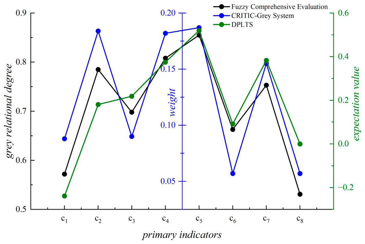
The proposed method directly calculates the mathematical expectation value of the double-sided probabilistic linguistic term set (DPLTS) for each indicator and identifies critical risk indicators by comparing their magnitudes. In contrast, the Fuzzy Comprehensive Evaluation Method ranks indicators based on the relative strength of their grey relational degree with the overall risk state, and the CRITIC–Grey System Theory Method determines important risk indicators by considering the weight of expert evaluations on each indicator. The results for identifying key primary indicators obtained by these three comparative methods are presented in Figure 7. Despite employing different risk evaluation dimensions, all three methods consistently identified excavation (c₅) and excavation support (c₄) as critical risk indicators. This convergence of findings confirms the credibility of the conclusions drawn by the proposed assessment method.

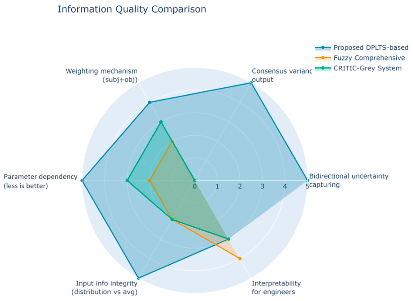
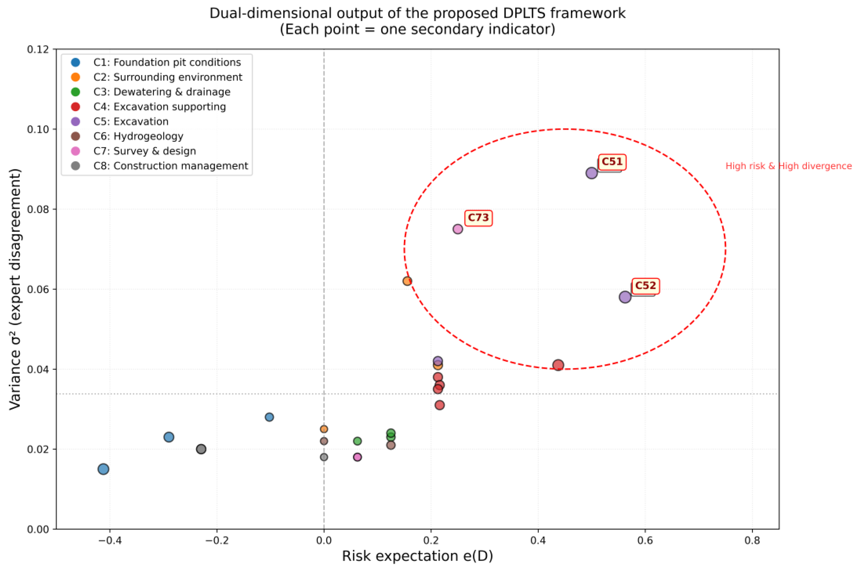
To clearly demonstrate the unique advantages of the DPLTS framework proposed in this study, this section systematically compares the evaluation information quality of the three methods presented in Section 5.3. We have formulated six evaluation criteria: (1) bidirectional uncertainty capturing, (2) consensus variance output, (3) combined subjective-objective weighting, (4) parameter dependency (lower is better), (5) input information integrity, and (6) interpretability. Each criterion was scored 1–5 based on three sources: theoretical definitions from literature [7,10,23], actual performance in this case study (e.g., DPLTS output variance σ² = 0.0503, while the others did not), and results in Table 12 and Section 5.2. The complete scoring rationale is visualized in Figure 8. To visually demonstrate the unique dual-output feature of the DPLTS framework (that is, simultaneously providing risk levels and expert consensus), we have drawn a two-dimensional scatter plot for 25 secondary indicators as shown in Figure 9 below. The x-axis represents the expected risk value. The e(D) data is directly taken from Table 7 (Equation 6), and the y-axis represents the variance σ², which is calculated using Equation 9 based on the original expert ratings.

Figure 9 shows that the DPLTS framework scores highest in five of six dimensions, with only interpretability slightly lower due to its mathematical formulation. It is the only method that captures bidirectional uncertainty (via dual probabilistic linguistic sets) and outputs a quantitative measure of expert disagreement (σ²). The scatter plot (Figure 9) visualises this dual-output capability. For example, indicators c₅₁ and c₅₂ fall in the upper-right quadrant (e(D) > 0.5, σ² > 0.05), indicating high risk and substantial expert divergence—such indicators require re-evaluation. Conversely, c₁₁ lies in the lower-left quadrant (negative e(D), low variance), suggesting low risk and strong consensus—a “safe” indicator. Thus, the DPLTS framework not only assigns risk levels but also flags controversial opinions, helping managers allocate resources rationally.

6. Conclusions

(1)

The DPLTS framework preserves both the mean and variance of expert ratings, enabling dual-dimensional risk characterization. In the case study, low overall variance (0.0527) confirms strong consensus, so the Level III (Moderate) classification reliably triggers routine controls. Conversely, high-variance indicators (e.g., c₅₁, σ² = 0.089) signal substantial disagreement despite moderate risk expectation—demanding targeted field review rather than simply increasing monitoring frequency. This distinction prevents overreaction to uncertain but not necessarily high-risk items.

(2)

The combined weighting model integrates objective weights with subjective BWM weights (strategic expert priorities). This mechanism ensures weights reflect both data-driven discriminability and engineering experience—avoiding pure objectivity that may ignore site context, and pure subjectivity that may amplify individual bias. In practice, higher combined weights directly translate to stricter site measures (e.g., excavation rate limits, dedicated supervision). Compared to uniform weights, BWM raises the overall risk expectation by ~23.7%, enhancing early warning. Moreover, the α coefficient (default 0.5) can be tuned to accommodate varying project risk tolerance, improving applicability across different engineering contexts.

(3)

Robustness is validated by entropy measures (variation < 4%), α-sensitivity (<4%), and consistent results against fuzzy comprehensive evaluation and CRITIC–Grey system. Limitations include a small expert panel (n = 4), non-membership set derived from dispersion rather than independent elicitation, and no real-time monitoring integration. Future work will incorporate larger panels and field data to strengthen engineering relevance.

References

1. Ru, G.; Zhang, Y.B.; Chen, W.Y.; Dong, P. Dynamic monitoring and deformation prediction in deep foundation pit engineering for urban renewal research overview. Water Resour. Hydropower Eng. 2025, 56, 15–17. [Google Scholar] [CrossRef]
2. Ghizlane, B.; Latifa, O.; Lahcen, B. Study of the Factors Affecting the Quality and Safety of Deep Excavations in Urban Areas of Casablanca-Settat Province-Morocco. Int. J. Adv. Sci. Eng. Inf. Technol. 2022, 12, 1989–1996. [Google Scholar] [CrossRef]
3. Wang, Z.Y.; Zhang, Y.P.; Zhang, S.L.; Gao, Y.C. Risk analysis of mechanical cross passage construction using work breakdown and fault tree. Proc. Inst. Civ. Eng. Forensic Eng. 2025, 178, 8–17. [Google Scholar] [CrossRef]
4. Abideen, D.K.; Kaltungo, A.Y.; Cheung, C.; Manu, P. Key information requirements for integrating building information modelling with operations and maintenance: A Delphi approach. J. Build. Eng. 2024, 98, 111445. [Google Scholar] [CrossRef]
5. Guo, J.; Qian, J.D.; Chen, J.; Yin, J.; Ke, X.F. Risk Identification and Evaluation of Deep Foundation Pit Construction for Metro Stations. J. Civ. Eng. Manag. 2017, 34, 32–38. [Google Scholar] [CrossRef]
6. Huang, L.P.; Wang, C.; Cui, B.B.; Zhou, H.M.; Wu, M.B.; Li, C.T. Employing an Interpretive Structural Modeling–System Dynamics Approach for Deep Foundation Pit Risk Assessment Model. ASCE-ASME J. Risk Uncertain. Eng. Syst. Part A Civ. Eng. 2024, 10, 04024004. [Google Scholar] [CrossRef]
7. Chen, Z.; Qiu, H.W.; Liu, J.Y.; Yang, S.Y. Risk assessment of deep foundation pits in subway stations based on variable fuzzy sets. China Saf. Sci. J. 2025, 35, 105–110. [Google Scholar] [CrossRef]
8. Fu, L.P.; Li, X.Q.; Wang, X.Q.; Li, M.N. Safety risk propagation in complex construction projects: Insights from metro deep foundation pit projects. Reliab. Eng. Syst. Saf. 2025, 257, 110858. [Google Scholar] [CrossRef]
9. Chen, D.W.; Zhang, J.L.; Ding, P.S.; Zhang, J.Q. Integrating knowledge management and BIM for safety risk identification of deep foundation pit construction. Eng. Constr. Archit. Manag. 2023, 30, 3242–3258. [Google Scholar] [CrossRef]
10. Xu, S.X.; Wu, B.; Zheng, W.Q.; Zhu, W.H.; Wang, Y.S.; Qiu, J.; Li, X. Risk assessment of subway deep foundation pit construction based on CRITIC and grey system theory: Taking the deep foundation pit of Daishan Station as an example. Sci. Technol. Eng. 2024, 24, 12325–12332. [Google Scholar] [CrossRef]
11. Gong, P.S.; Guo, H.X.; Huang, Y.Y.; Guo, S.Y. Safety risk evaluations of deep foundation construction schemes based on imbalanced data sets. J. Civ. Eng. Manag. 2020, 26, 380–395. [Google Scholar] [CrossRef]
12. Zhang, Z.Y.; Deng, Z. Extension AHP-Based Assessment of Safety Risk Levels in Subway Deep Excavation Construction. J. Civ. Eng. Urban Plan. 2023, 5, 48–60. [Google Scholar] [CrossRef]
13. Wu, B.; Wan, Y.; Xu, S.X.; Zhao, C.X.; Liu, Y.; Zhang, K. A Multi-Source Intelligent Fusion Assessment Method for Dynamic Construction Risk of Subway Deep Foundation Pit: A Case Study. Sustainability 2023, 15, 10162. [Google Scholar] [CrossRef]
14. Ehsan, M.; Mehdi, P.; Hesam, S.T.; Ali, F. Reliability analysis and Risk Assessment of Deep Excavations using Random-Set Finite Element Method and Event Tree Technique. Transp. Geotech. 2021, 29, 100560. [Google Scholar] [CrossRef]
15. Wu, B.; Xia, Q.; Liu, C.; Xie, Y.D.; Huang, W. Multivariate Information Fuzzy Extension Risk Assessment Model for Deep Foundation Pits in Richly Water-Saturated Soft Soil and Its Application. J. Saf. Environ. 2024, 24, 1–10. [Google Scholar] [CrossRef]
16. Wu, B.; Zhao, R.; Meng, G.W.; Chen, H.H.; Huang, W.; Liu, J.L.; Cheng, Y. Safety Risk Assessment of Asymmetric Construction of Deep Foundation Pit of Subway Based on Fuzzy Theory. J. Civ. Environ. Eng. 2022, 44, 8–15. [Google Scholar] [CrossRef]
17. Wei, D.J.; Xu, D.S.; Zhang, Y. A fuzzy evidential reasoning-based approach for risk assessment of deep foundation pit. Tunn. Undergr. Space Technol. 2020, 97, 103232. [Google Scholar] [CrossRef]
18. Khan, R.N.; Khan, M.S.A.; Mashwani, W.K.; Ibrar, M.; Senapati, T.; Moslem, S. Multi-Criteria Decision Making Model For Hotel Selection Problem Under Complex Dual Hesitant Fuzzy Information. Appl. Artif. Intell. 2024, 38, 2300215. [Google Scholar] [CrossRef]
19. Krishankumar, R.; Mishra, A.R.; Rani, P.; Ecer, F.; Zavadskas, E.K.; Ravichandran, K.S.; Gandomi, A.H. Two-Stage EDAS Decision Approach with Probabilistic Hesitant Fuzzy Information. Informatica 2025, 36, 65–97. [Google Scholar] [CrossRef]
20. Torra, V. Hesitant fuzzy sets. Int. J. Intell. Syst. 2010, 25, 529–539. [Google Scholar] [CrossRef]
21. Zhu, B.; Xu, Z.S. Probability-hesitant fuzzy sets and the representation of preference relations. Technol. Econ. Dev. Econ. 2018, 24, 1029–1040. [Google Scholar] [CrossRef]
22. Pang, Q.; Wang, H.; Xu, Z.S. Probabilistic linguistic term sets in multi-attribute group decision making. Inf. Sci. 2016, 369, 128–143. [Google Scholar] [CrossRef]
23. Xie, W.Y.; Xu, Z.S.; Ren, Z.L. Dual probabilistic linguistic term set and its application on multi-criteria group decision making problems. In Proceedings of the 2017 IEEE International Conference on Industrial Engineering and Engineering Management (IEEM), Singapore, 10–13 December 2017; pp. 1469–1474. [Google Scholar] [CrossRef]
24. Bilal, M.; Popa, I.L. A novel hesitant fuzzy tensor-based group decision-making approach with application to heterogeneous wireless network evaluation. Sci. Rep. 2025, 15, 30734. [Google Scholar] [CrossRef] [PubMed]
25. Ameen, Z.A.; Salih, H.F.M.; Alagal, W.; Asaad, B.A. q-Fractional Hesitant Fuzzy Multicriteria Decision-Making Approaches for Uncertain Power System Performance Evaluation. Energy Sci. Eng. 2025, 13, 5311–5337. [Google Scholar] [CrossRef]
26. Bashir, Z.; Bashir, Y.; Rashid, T.; Ali, J.; Gao, W. A Novel Multi-Attribute Group Decision-Making Approach in the Framework of Proportional Dual Hesitant Fuzzy Sets. Appl. Sci. 2019, 9, 1232, Correction in Appl. Sci. 2025, 15, 11818. https://doi.org/10.3390/APP152111818. [Google Scholar] [CrossRef]
27. Pujara, S.; Kumar, S. Knowledge and accuracy measures for dual hesitant fuzzy sets with their applications in pattern recognition and multiple attribute decision making. Frankl. Open 2026, 14, 100476. [Google Scholar] [CrossRef]
28. Qi, X.W.; Zhang, J.L.; Liang, C.Y. A Bilateral Probabilistic Linguistic Multi-Criteria Decision-Making Method Based on the Extended Least Common Multiple of Hesitant Fuzzy Elements and Fuzzy Entropy. Syst. Eng.—Theory Pract. 2022, 42, 2243–2257. [Google Scholar] [CrossRef]
29. Meng, L.Y.; Li, L.Q.; Xie, W.X.; Li, Y.S.; Liu, Z.X. Time-sequential hesitant fuzzy entropy, cross-entropy and correlation coefficient and their application to decision making. Eng. Appl. Artif. Intell. 2023, 123, 106455. [Google Scholar] [CrossRef]
30. Wu, B.; Chen, H.H.; Huang, W.; Meng, G.W.; Li, X.L.; Wan, R.Q. Risk assessment of water and sand gushing in deep foundation pit based on the FAHPGRA theory. J. Railw. Sci. Eng. 2021, 18, 2209–2216. [Google Scholar] [CrossRef]
31. Alijani, M.; Feizabadi, Y.; Goudarzi, M. Comparative analysis of paddy cultivation sustainability through integrating eco-efficiency and best-worst method approaches. J. Agric. Food Res. 2025, 19, 101479. [Google Scholar] [CrossRef]
32. Wang, F.; Pan, Y.; Xu, G.L.; Wei, Q. Probabilistic linguistic multi-attribute group decision making method considering the important degrees of experts and attributes. Expert Syst. Appl. 2025, 265, 125899. [Google Scholar] [CrossRef]
33. GB 50652-2011; Code for Risk Management of Underground Works in Urban Rail Transit. Ministry of Housing and Urban-Rural Development of the People’s Republic of China & General Administration of Quality Supervision, Inspection and Quarantine of the People’s Republic of China: Beijing, China, 2011.
Figure 1. Risk assessment process.
Buildings 16 02568 g001
Figure 2. Stratigraphic section diagram.
Buildings 16 02568 g002
Figure 3. Risk Index System for Deep Foundation Pit Construction.
Buildings 16 02568 g003
Figure 4. Delphi validation of the 25 secondary risk indicators.
Buildings 16 02568 g004
Figure 5. Pearson correlation matrix of the 25 secondary indicators based on the four experts’ ratings.
Buildings 16 02568 g005
Figure 6. The objective weight changes in secondary indicators based on different α values.
Buildings 16 02568 g006aBuildings 16 02568 g006b
Figure 7. Identification results of key indicators for the three methods.
Buildings 16 02568 g007
Figure 8. Information quality comparison among the three risk assessment methods.
Buildings 16 02568 g008
Figure 9. Dual-dimensional output of the proposed DPLTS framework.
Buildings 16 02568 g009