A Pipeline for Topology Optimization of Reinforced-Concrete Frames: A Systematic Approach for Ground-Structure Generation, Selection, and Optimization

Abstract

The topology optimization of reinforced-concrete (RC) building frames is relatively underexplored compared to steel structures, partly due to the lack of a systematic approach to generate and select ground structures (GS). Existing methods often use less systematic GS strategies, limiting efficient exploration of the vast and sparse design space shaped by large bay widths and story heights. This work addresses this gap by providing a comprehensive and systematic pipeline tailored for RC frames. The key contributions are: (1) development of a GS generation framework that systematically enumerates all feasible RC frame configurations within user-defined constraints, (2) introduction of a candidate GS selection map, a surrogate-based tool employing graph-based Latin hypercube sampling (LHS) and sparse Gaussian Process (GP) models, which predicts compliance early and strategically guides candidate selection, reducing computational cost by limiting full finite-element evaluations to the order of ${10}^3$ out of up to ${10}^5$ generated frames while serving as a reference for understanding design-parameter influences; and (3) implementation of an integrated topology-optimization pipeline applying particle swarm optimization (PSO) to selected candidates, achieving efficient compliance minimization with reduced computational effort. The complete workflow—which spans GS generation, surrogate-based candidate selection, and iterative optimization—is implemented and validated in two design domains with width-to-height aspect ratios of 1:1 and 1:1.5 and generates 438,984 and 104,032 different frame configurations, respectively. These selected candidates undergo PSO-based optimization, yielding designs with volume fractions below 0.55 and preserving critical floor beams, demonstrating the framework’s ability to identify structurally efficient stiffness-driven RC frame topologies for early-stage screening. The framework is designed as an extensible foundation that can be coupled with more detailed member-level design checks and nonlinear RC analysis in future work, rather than replacing full reinforced-concrete design procedures.

1. Introduction

Topology optimization seeks to determine the most efficient material distribution within a predefined design domain, subject to applied loads, boundary conditions, and specific performance criteria. The nature of the objective function plays a central role in shaping the optimal structure. Two known objective formulations are stress minimization and compliance minimization, each producing distinct structural layouts and serving different engineering priorities.

Stress minimization focuses on limiting material stresses to remain within allowable limits, resulting in designs that are typically more redundant, with multiple load paths. This often results in structures composed of many slender members. While beneficial for robustness and reliability, especially in structures where multiple load paths are desirable, the stress-based approach is computationally intensive due to the complexity of satisfying local stress constraints in iterative design updates.

Compliance minimization, in contrast, aims to reduce the total strain energy or, equivalently, maximize global stiffness. This method tends to produce fewer structural members with larger cross-sectional areas, leading to more efficient yet sparse structural configurations. Compliance-based designs are computationally simpler and more scalable, making them a popular choice in practical applications. From the perspective of reinforced-concrete (RC) structures, compliance minimization is often more suitable. RC members are subject to constructability constraints such as minimum cross-sectional dimensions required to accommodate reinforcement and concrete aggregate. Therefore, a design that favors fewer, thicker members aligns better with real-world RC detailing requirements. On the other hand, for frame-type or steel structures where member slenderness is more acceptable and structural redundancy is desirable, stress-based formulations may be preferred despite their higher computational cost.

Topology optimization of structures with a continuum domain starts with a solid surface or volumetric object, as the approach is density-based. For discrete structures, which are mainly framed, however, the ground structure is used. A ground structure serves as a starting structure for an optimization task, where iterative adjustments are made to its members and topology to achieve an optimal structure [1]. Due to the significant influence of node positions and the number of connected members on the initial ground structure, various studies have been conducted to address both computational burden and optimality [2,3,4]. Beyond the choice of the initial ground structure, several works have emphasized that sampling strategy and structural descriptors must be judged not only by nominal coverage of the design space but also by the reliability of the final design decisions, particularly near the optimum, in contexts such as structural reliability analysis and ground-structure candidate filtering [5,6,7,8].

A fully connected ground structure, in which every node is connected to every other node by all possible connections, leads to a complex optimization process and requires significant computational resources, including considerable computer capacity and time [9]. Overlapping members, inclusion of slender members, and structural instability pose challenges to overcome when contemplating such a ground structure [10].

A second approach is addressed in various ways, such as gradually removing unfit members and adding fit members, or generating levels of connectivity to include the preferred number of members based on the required solution accuracy [6,11,12].

Ranalli et al. [7] employed a foundational framework to reduce the overall installed expenses of steel frame structures. Sequentially, they implemented topology and size optimizations as outer and inner loops. Sokol [9] utilized a foundational structure for conducting topology optimization of large-scale trusses. His methodology began by prioritizing shorter member-to-node connections and gradually incorporated longer potential members. Following his approach, as new members were potentially added, less-critical existing members were removed.

The aforementioned approaches, however, have not been further extended to RC structures due to the orthogonal orientation of member connectivity. Reinforced-concrete structures have undoubtedly earned significant attention in the research community, both as reinforced concrete [13,14,15] and as composed of structural steel [16,17], indicating that such optimization is of great importance. In parallel, recent developments in low carbon and engineered cementitious composites further increase the incentive to design material efficient RC systems, as mechanical properties, long term behavior, and life cycle performance of advanced concretes are increasingly quantified in the literature [18].

Reinforced-concrete (RC) building frames typically exhibit relatively sparse connectivity, yet the number of potential frame configurations within a given spatial domain can be extremely large. This arises from combinatorial variations in node placement, bay width, and story height parameters that are bounded by constructional constraints but still allow for a vast number of feasible layouts. Such complexity calls for a systematic and efficient approach to generating and selecting candidate ground structures suitable for topology optimization, particularly because the optimization process involves repeated structural reanalysis and is computationally demanding. The scarcity of research that explicitly addresses this challenge within the context of RC frames further highlights the need for a targeted methodology. At the same time, earlier studies on steel frames and truss lattices have shown that ground structure generation, candidate pruning, and ranking strategies directly affect the reliability of the final layout, especially when very large combinatorial design spaces are involved. This motivates a pipeline in which ground structure enumeration, sampling, surrogate prediction, and final optimization are explicitly co designed rather than treated as independent steps.

Conventional ground structure-based topology-optimization approaches generally begin with a single predefined frame and seek to optimize member connectivity within that fixed layout. Whether fully connected (where all nodes are linked), neighbor-based (where connections are restricted to adjacent nodes), or growth-based (where elements are progressively added during optimization), these methods share a core limitation: they operate within the confines of one initial ground structure. As a result, they are inherently unable to capture the full diversity of frame configurations permitted by RC design constraints, such as minimum bay width and story height. This restricts their ability to explore realistic yet diverse structural possibilities.

The approach proposed in this work addresses this limitation by systematically enumerating all feasible RC frame configurations over a given domain, subject to geometric and constructional constraints. Each configuration yields a distinct, sparse, and structurally meaningful ground structure.

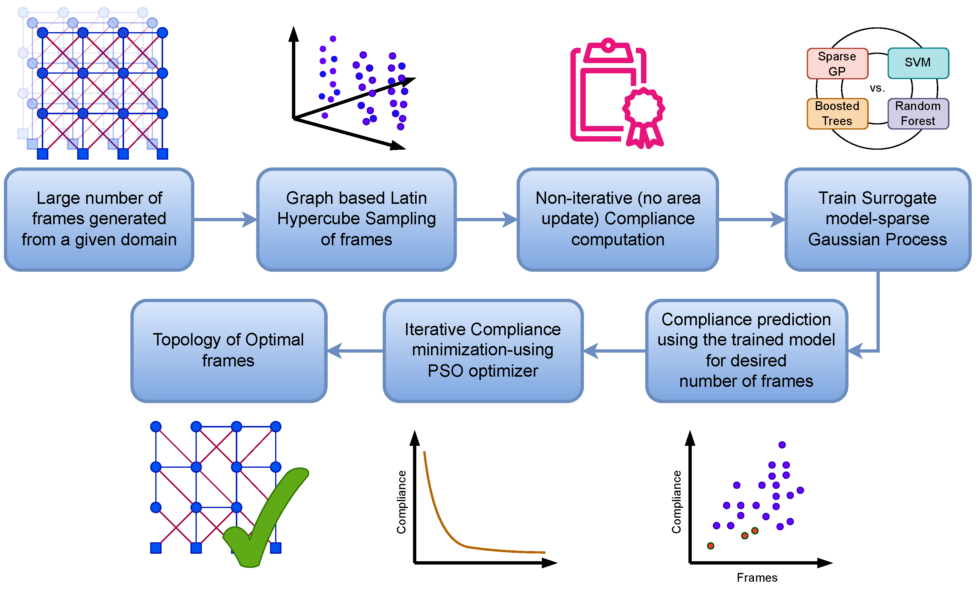
This work addresses the challenge by proposing a structured methodology for generating and optimizing RC frame configurations. The remainder of the paper is organized as follows:

• Section 2 introduces a systematic ground-structure generation method,
• Section 3 outlines the overall methodological framework,
• Section 4 presents the formulation of compliance minimization and its optimization requirements,
• Section 5 explores the use of surrogate models for rapid compliance prediction to support candidate selection,
• Section 6 applies full topology optimization to the selected candidate structures,
• Finally, Section 7 discusses implications and future directions.

Methodologically, this work intersects three related but distinct strands of literature: (i) ground-structure-based topology optimization, which provides the foundations for member pruning, connectivity control, and stiffness-driven layouts; (ii) surrogate-assisted structural optimization, in which sampling strategies and learning models guide the selection of high-value candidates from very large design spaces; and (iii) RC member and frame design feasibility, which governs section dimensions, reinforcement, and code compliance. Several references from other engineering domains are therefore cited not as direct RC analogs but as methodological parallels illustrating how design-space filtering, multiobjective trade-offs, and optimization stability are handled in optimization-driven design. Their role here is to contextualize the proposed pipeline within a broader class of optimization methods rather than to substitute for RC-specific verification studies.

Several cross-domain studies inform the methodological choices adopted in this pipeline. Machine learning–finite-element mesh optimization frameworks for excavation-induced ground settlement [19] and adaptive measurement-based substructure identification methods [20] demonstrate the feasibility of coupling FE-based simulations with surrogate models for design-space filtering under computational constraints. Multiobjective optimization using response surface methods and NSGA-II applied to pressure-maintaining valves [21] and topology optimization of cooling channels based on swarm intelligence [22] illustrate how swarm-based algorithms can navigate complex trade-offs in topology and sizing problems. Diameter-adjustable mandrel optimization with domain knowledge integration [23] and aluminum bicycle pedal crank topology optimization using laser powder bed fusion [24] provide examples of integrating domain knowledge—such as manufacturability constraints and feature-angle limits—directly into the ground-structure generation stage. Three-dimensional high-fidelity mesoscale modeling for concrete [25] illustrates the level of geometric detail required for fully realistic RC simulations at the material scale.

These references are cited not as direct RC analogs but as methodological parallels that support specific arguments about FE–ML coupling, PSO robustness in topology optimization, surrogate-guided design selection, and constructability-aware generation. Their role here is to contextualize the proposed pipeline within a broader class of optimization methods rather than to substitute for RC-specific verification studies.

2. Enumerative RC Frame Ground-Structure Generation

This section describes the systematic enumeration of all feasible RC frames within a given domain subject to constructability constraints. Each nodal location interval yields a distinct set of frames. Unlike existing fully connected approaches, only meaningful orthogonal and limited-diagonal connectivity is permitted, consistent with RC construction practice.

Given a domain space, bay width, and story height bounds, all possible nodes are first generated. Each set of nodal location intervals along the existing axes returns a different set of frames. Basic ground-structure frame, formed by connecting nodes orthogonally, is generated for each set of nodes.

2.1. Nodes

Given a $W\times H$ frame domain, where:

The allowable dimensions for bays and stories are defined by:

$$\begin{array}{cc}\hfill & W=\{w_i\mid w_{\min }\le w_i\le w_{\max }\},\hfill \\ \hfill & H=\{h_j\mid h_{\min }\le h_j\le h_{\max }\}.\hfill \end{array}$$

(1)

where:

• W: Set of allowable bay widths,
• H: Set of allowable story heights,
• $w_i$: Width of the $i\mathrm{th}$ bay option,
• $h_j$: Height of the $j\mathrm{th}$ story option.

For given nodal location intervals $w_{\mathrm{int}}$ and $h_{\mathrm{int}}$, discrete nodal locations are defined within the frame domain while generating nodes for multiple different sets of frames. Accordingly, bay sequences and story sequences are generated.

2.1.1. Bay Sequences

$$B=\left\{\mathbf{B}=(b_1,\dots ,b_{N_b})\mid b_k\in W,W_{\max }-w_{\min }\le {\displaystyle \sum _{k=1}^{N_b}}{b}_k\le W_{\max }\right\}.$$

(2)

where:

• $\mathbf{B}$: Sequence of bay widths,
• $b_k$: Width of the $k\mathrm{th}$ bay,
• $N_b$: Number of bays,
• $W_{\max }$: Maximum total domain width,
• $w_{\min }$: Minimum allowable bay width.

2.1.2. Story Sequences

$$S=\left\{\mathbf{S}=(s_1,\dots ,s_{N_s})\mid s_l\in H,H_{\max }-h_{\min }\le {\displaystyle \sum _{l=1}^{N_s}}{s}_l\le H_{\max }\right\}.$$

(3)

where:

• $\mathbf{S}$: Sequence of story heights,
• $s_l$: Height of the $l\mathrm{th}$ story,
• $N_s$: Number of stories,
• $H_{\max }$: Maximum total domain height,
• $h_{\min }$: Minimum allowable story height.

2.1.3. Nodal Grid Generation

Each nodal grid $\mathcal{N}(\mathbf{B},\mathbf{S})$ is defined by the cumulative positions of bays and stories:

$$\begin{array}{cc}& x_i={\displaystyle \sum _{k=1}^{i-1}}{b}_k,i=1,\dots ,N_b+1,\hfill \\ & y_j={\displaystyle \sum _{l=1}^{j-1}}{s}_l,j=1,\dots ,N_s+1,\hfill \end{array}$$

$$G=\left\{N(\mathbf{B},\mathbf{S})\mid \mathbf{B}\in B,\mathbf{S}\in S\right\}.$$

(4)

where:

• G: Set of all feasible nodal grids,
• $N(\mathbf{B},\mathbf{S})$: Nodal grid from bay and story sequences,
• $x_i$: Horizontal position of grid line i,
• $y_j$: Vertical position of grid line j.

2.1.4. Number of Nodes

$$N_{\mathrm{nodes}}=(N_b+1)(N_s+1).$$

(5)

where:

• $N_{\mathrm{nodes}}$: Total number of nodal intersections in the 2D grid.

2.1.5. Perturbable Node Set

To preserve the total floor area of each slab, nodal perturbations are restricted so that the grid lines defining the outer slab boundaries remain fixed while the interior nodes may shift laterally. In this context, edge nodes refer to nodes on the leftmost and rightmost vertical axes, and base nodes on the bottommost horizontal axis; these are excluded from perturbation to avoid changing the overall frame footprint or effectively transforming one ground structure into another configuration. Consequently, nodes that are allowed to perturb horizontally exclude:

• Nodes on the leftmost vertical axis ($i=0$),
• Nodes on the rightmost vertical axis ($i=N_b$),
• Nodes on the bottommost horizontal axis ($j=0$).

Thus, the set of perturbable nodes is as follows:

$$\mathcal{P}=\left\{(i,j)\mid i=1,\dots ,N_b-1,j=1,\dots ,N_s\right\}.$$

(6)

2.1.6. Bay Width Constraint Under Perturbation

To ensure valid configurations under perturbation:

$$w_{\min }\le b_k\le w_{\max }.$$

(7)

Let $\delta$ be the magnitude of the horizontal perturbation. A node $(i,j)\in \mathcal{P}$ can:

• Move left by $\delta$ if both $b_{i-1}$ and $b_i$ remain within bounds,
• Move right by $\delta$ under the same condition,
• Or remain in place.

In addition to the bounds on bay widths, story heights, and nodal perturbations, an explicit angular feasibility constraint is imposed during ground-structure generation to avoid impractical inclined members. A minimum angle threshold of $\theta ={30}^{\circ }$ with respect to the horizontal axis is prescribed. Candidate members that would create excessively shallow diagonals are therefore excluded from the admissible set, reducing geometries that are prone to reinforcement congestion, poor force transfer, or limited structural usefulness in reinforced-concrete frame systems. This angular filter complements the width and height bounds by introducing a quantitative feasibility criterion at the ground-structure generation stage rather than relying only on qualitative arguments about constructability.

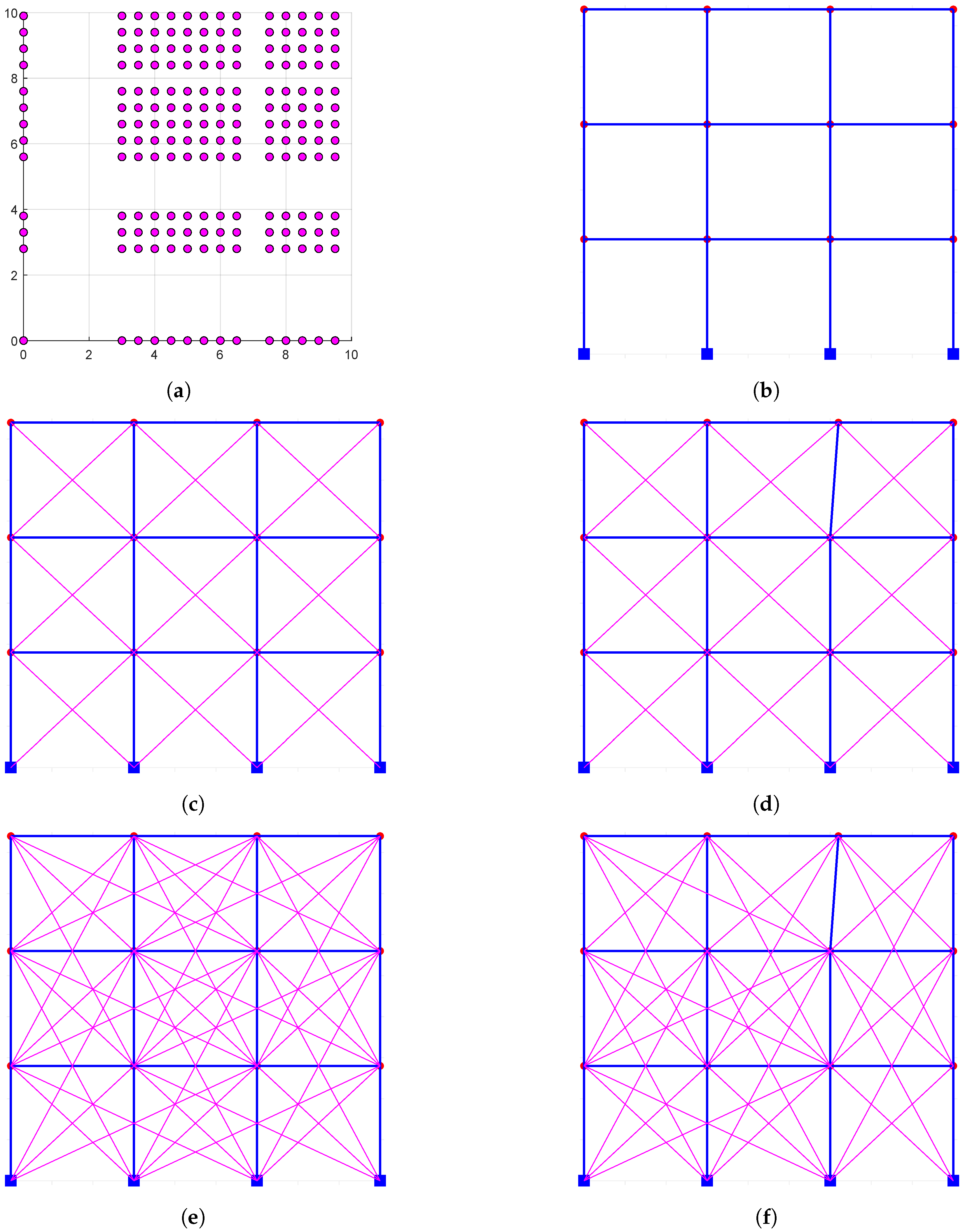
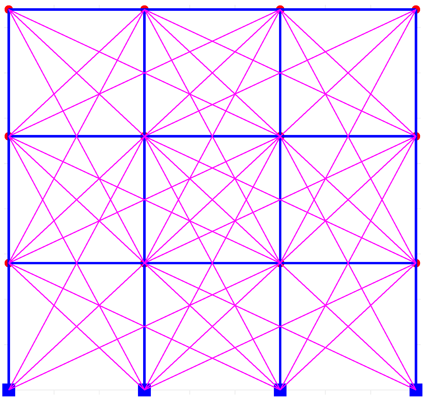
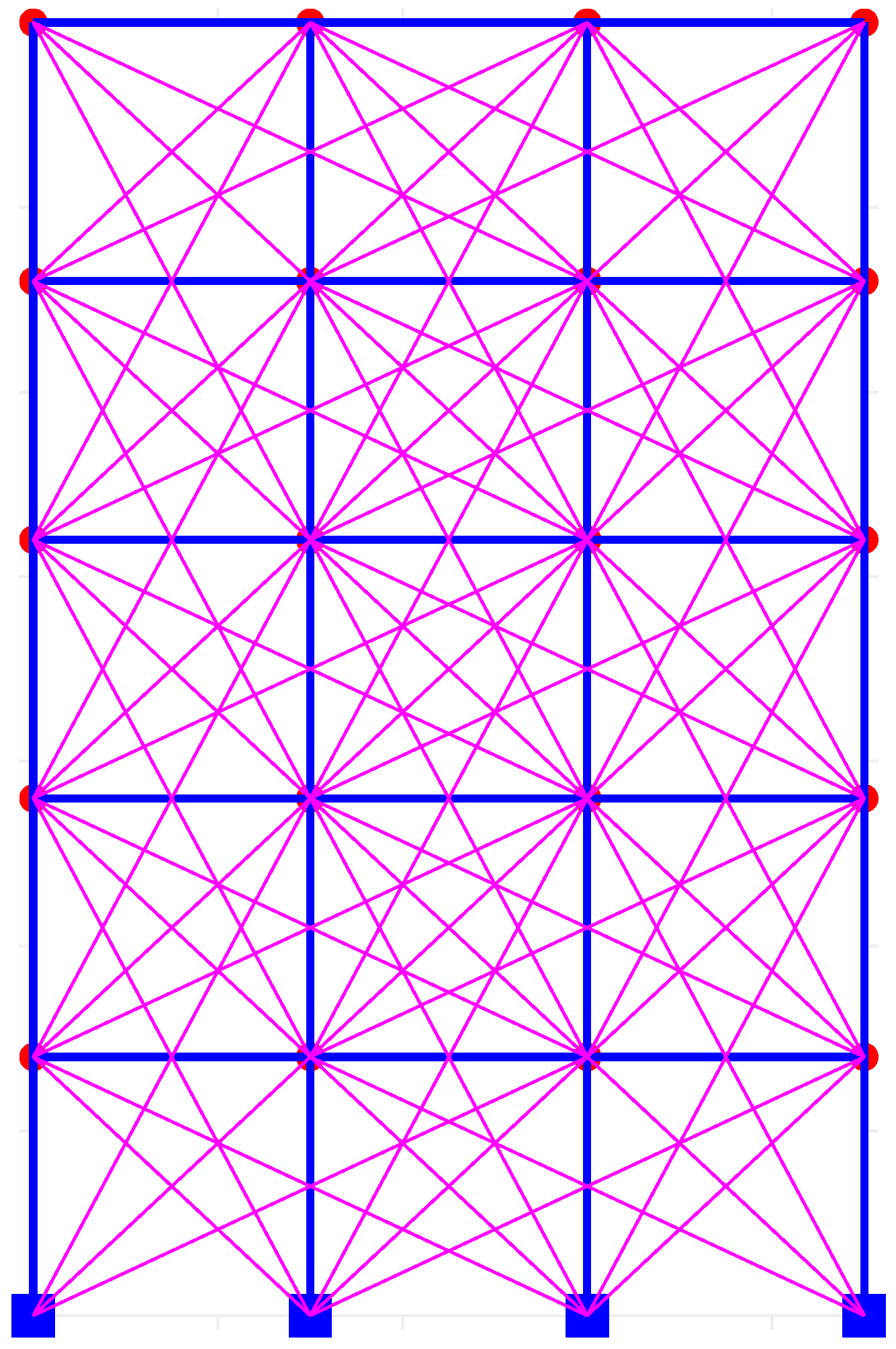
Figure 1a shows all nodes generated for a given pair of bay width and story height interval ranges. Subsets of these nodes connect to result in a large number of possible frames. For a $[w_{min},w_{max}]$ bay width bound of [3 m, 7 m] and a $[h_{min},h_{max}]$ story height bound [2.8 m, 4 m] and 10 m by 10 m domain size, and an interval range of 0.5 m for both bay width and story height used, and also a $\delta$ 0.2 m lateral nodal perturbation is allowed, 26208 ground structures that result in a total of 438,984 frames (both perturbed and normal) are generated. Regardless of the connectivity level, for each chosen connectivity level, such a number of frames is generated. This is because the number of frames is decided based on Level 1 connectivity and perturbation. The rest levels change only the connectivities of these resulted frames. Variation in the interval range corresponds to the fineness or coarseness of mesh grids in the mesh grid approach. Smaller interval ranges produce nearly similar frames. One of the top interior nodes is perturbed to the right in Figure 1d,f.

2.2. Elements

The connectivity levels are built on top of basic GS connectivity, which connects nodes orthogonally as seen in Figure 1b. The connectivity levels, therefore, dictate the diagonal nodal connectivity.

Level 1 connectivity is defined by linking nodes within the same bay-story box via immediate diagonal connections along the frame axes.

Level 2 connectivity extends this by allowing diagonal connections to nodes in the adjacent bay-story boxes in all directions within the plane, effectively permitting each node to connect within a $3\times 3$ nodal grid. This level captures more complex interactions and increases the design space.

Perturbed Level 1 connectivity is formed by allowing perturbation of node/s laterally on each of the frames generated with Level 1 connectivity. When nodes are perturbed, this allows for the emergence of inclined members, enabling a more versatile structural layout.

Perturbed Level 2 connectivity is formed by allowing perturbation of node/s laterally on each of the frames generated with Level 2 connectivity.

The proposed ground-structure generation method captures all possible connections for the resolution defined by the selected nodal location interval. Topology optimization can be applied to structures with Level 1, Level 2, or higher levels of connectivity, including fully connected frames. However, in reinforced-concrete (RC) framed structures—where members cannot be made as small as in steel frames—excessive connectivity may lead to element congestion, slenderness issues, and increased construction complexity. As such, limiting connectivity to Level 2 could generally be more appropriate and practical for RC frames. Compared with standard fully connected truss ground structures, which allow arbitrary member orientations between any pair of nodes, the orthogonal initialization adopted here restricts members to align with bays and stories and to a limited set of diagonal patterns consistent with RC frame construction. This reduces the number of extremely slender and intersecting members, mitigates instability and congestion issues highlighted in steel truss studies [1,2,3,4,26,27], and produces ground structures whose connectivity is mechanically closer to practical RC frames. Moreover, elements for the above Level 1 connectivity consider the removal of longer elements based on proximity among them, measured in degrees.

For 2D case the total number of elements $E_{2D}$ for Level 1 connectivity is given by:

E_2D = N_bN_s + (N_b + 1)N_s + 2N_bN_s.

(8)

The first, second, and third components of the summation represent the number of beam, column, and diagonal elements, respectively.

2.3. Frames

The total number of frames is calculated below as $N_{\mathrm{layouts}}$.

Let $p_{i,j}\in \{1,2,3\}$ denote the number of valid perturbation options at node $(i,j)$. Then:

$$N_{\mathrm{layouts}}=\prod _{(i,j)\in \mathcal{P}}{p}_{i,j}.$$

(9)

where:

• $N_b,N_s$: Number of bays and stories,
• $\mathcal{P}$: Set of perturbable node indices,
• $b_k$: Width of the $k\mathrm{th}$ bay,
• $\delta$: Perturbation magnitude,
• $p_{i,j}$: Valid perturbation options at node $(i,j)$,
• $N_{\mathrm{layouts}}$: Total number of unique perturbed layouts.

The orthogonal initialization and Level 1/Level 2 connectivity adopted here differ fundamentally from fully connected truss ground structures commonly used in steel topology optimization. By restricting diagonal members to 30° minimum angles and capping connectivity at Level 2, the framework reduces element congestion and produces layouts mechanically closer to practical RC frames. This design choice parallels manufacturability-aware topology-optimization practices in other engineering domains, where feature-angle and joint-complexity constraints are imposed during ground-structure generation rather than as post-processing filters, ensuring that the initial candidate set reflects practical fabrication limits.

3. Methodology

3.1. Reinforced-Concrete Material Property Representation

While plastic analysis-based topology-optimization methods exist and can simplify topology optimization, particularly for steel structures, by assuming full plasticity of each member without requiring detailed stiffness matrix computations, these approaches are less straightforward for RC. For example, the GRAND framework developed by [28] efficiently uses plastic collapse mechanisms to directly find optimal steel topologies under ultimate load conditions, bypassing the complexities of elastic compliance minimization. This works well for steel because its behavior closely matches ideal plasticity without complex cracking or tension softening.

For RC systems, however, the nonlinear response under service and ultimate loads is governed by cracking, tension softening, reinforcement yielding, and confinement effects that have been extensively investigated using detailed finite-element models and experimental validation, for example, in studies of RC beams and columns under monotonic, cyclic, and post fire loading [13,14,16,17,29]. These works illustrate the level of modeling detail required to capture realistic RC behavior, and therefore define a natural second stage beyond the linear elastic screening considered here.

However, RC’s nonlinear behavior, such as cracking, tension softening, and complex elasto-plastic responses, makes applying full plasticity assumptions at the conceptual stage more challenging and less practical. Therefore, despite the elegance and efficiency of plastic-collapse-based methods for steel, the elastic approach remains preferable for RC topology optimization. It provides a simpler, computationally efficient framework consistent with standard civil engineering practice, where serviceability and load-path identification are the main goals.

Both elastic and elasto-plastic analysis frameworks can be incorporated into structural optimization, depending on the design stage and objectives. Linear-elastic analysis assumes small deformations and neglects geometric nonlinearity, making it suitable for early-stage conceptual design. It satisfies equilibrium and compatibility conditions and aligns with standard civil engineering practices. In contrast, elasto-plastic analysis captures nonlinear material behavior and ultimate capacity, but is less common in topology optimization due to its computational complexity. Still, it is essential for capturing realistic failure modes and ensuring safety under extreme loading conditions.

In the case of RC building structures, the initial goal is to ensure satisfactory performance under service loads, thus keeping the structure in the elastic range. This justifies the use of an elastic representation of RC during the first stage of ground-structure topology optimization, where the objective is to minimize compliance and identify efficient load paths with minimal material use. However, under extreme or ultimate loading conditions, the structure must remain stable and ductile, which requires considering the elasto-plastic behavior of RC materials, including steel yielding and concrete cracking.

From a member-level verification perspective, realistic RC behavior under service and ultimate loads is governed by cracking, tension softening, reinforcement yielding, and confinement effects that have been extensively investigated using detailed finite-element models and experimental validation, for example, in studies of RC beams and columns under monotonic, cyclic, and post-fire loading [13,14,16,17,29]. These works illustrate the level of modeling detail required to capture realistic RC behavior and therefore define a natural second stage beyond the linear-elastic screening considered here. Studies on composite RC members, shear connectors in steel-concrete systems, and connection behavior under seismic loading further emphasize that joint-level verification, detailing feasibility, and ductility assessment require nonlinear FE models with explicit reinforcement and contact modeling.

Detailed code-based checks on steel yielding, concrete cracking, shear capacity, and ultimate compressive strength are therefore reserved for subsequent member-level design verification rather than being enforced during the topology-optimization stage. The present formulation deliberately positions the proposed pipeline as an early-stage screening and layout tool that identifies promising RC frame topologies under service-level stiffness criteria, while recognizing that ultimate-limit-state verification, crack-width control, and detailed reinforcement design must follow using established nonlinear and code-based approaches, such as those in [13,15,27,29,30].

In the broader RC literature, several works have employed data driven models such as extreme learning machines and artificial neural networks to predict compressive strength and long term material behavior, including hybrid ELM–grey wolf optimizers and ANN based assessments of fly ash and silica fume concretes [31,32]. These approaches target material scale properties under specific mix designs, whereas the surrogate component of the present pipeline operates at the structural frame level, predicting global compliance over a combinatorial space of ground structures and feeding directly into topology optimization.

3.2. Method Followed

Graph-based Latin hypercube sampling (LHS) selects a representative subset of ground structures. Finite-element analysis computes compliance for these samples. A sparse Gaussian Process (GP) surrogate is trained on these data and validated using held-out frames.

The trained surrogate predicts compliance for unevaluated frames. Candidates with minimum predicted compliance are identified for subsequent PSO optimization.

A subset of these candidates from each category is then selected and subjected to PSO, through which the final optimal configuration is determined.

The proposed pipeline is presented in Figure 2. Each step is executed sequentially that finally leads to the candidate optimal RC frame.

4. Compliance-Based Optimization

4.1. Objective Function

The compliance minimization problem is formulated as

$$\begin{array}{cc}\hfill \underset{a}{\min }& C\left(a\right)=f^{T}U\left(a\right),\hfill \\ \hfill \mathrm{s}.\mathrm{t}.& K\left(a\right)U\left(a\right)=f,\hfill \\ \hfill & a_{\min }\le a\le a_{\max },\hfill \\ \hfill & {\displaystyle \frac{1}{n}}{\displaystyle \sum _{i=1}^n}{a}_i\le V_f.\hfill \end{array}$$

(10)

where:

• C: Compliance (objective to minimize),
• $f\in {\mathbb{R}}^m$: External force vector,
• $U\in {\mathbb{R}}^m$: Displacement vector,
• $K\left(a\right)\in {\mathbb{R}}^{m\times m}$: Global stiffness matrix (depends on a),
• $a={[a_1,a_2,\dots ,a_n]}^T\in {\mathbb{R}}^n$: Vector of design variables (e.g., element densities),
• $a_{\min },a_{\max }\in \mathbb{R}$: Lower and upper bounds on a,
• n: Number of finite elements,
• $V_f\in (0,1]$: Prescribed maximum volume fraction.

4.2. Design Variables

The primary design variable is cross-sectional area. Since stiffness depends on moment of inertia I, which for rectangular sections is a function of width and height, height h is related to area A through regression to reduce the number of independent variables. Width is then computed directly from height.

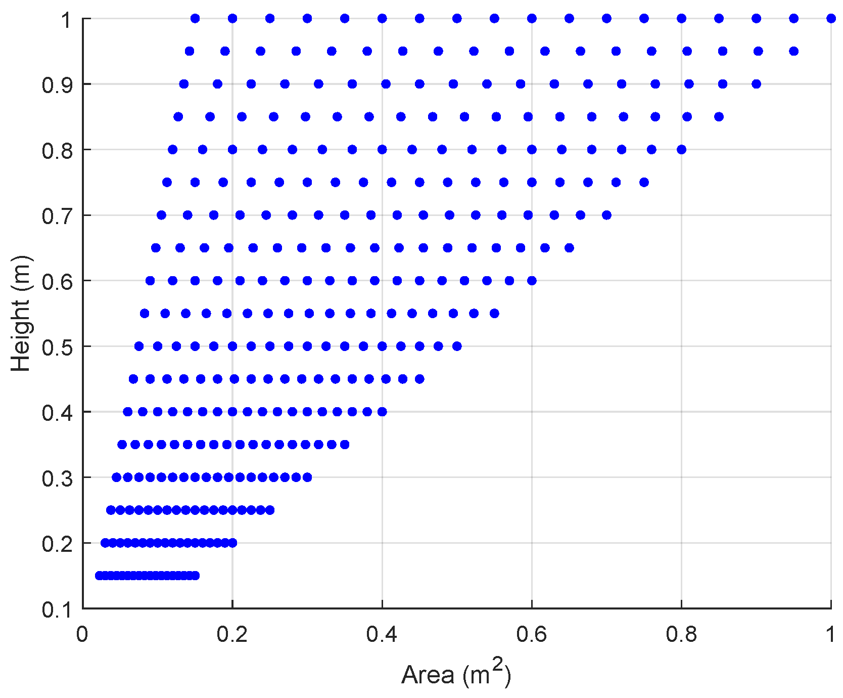
Accordingly, 324 data points for height and area are generated between a height of 0.15 m and 1 m with a 5 cm interval for workability as shown in Figure 3. A regression model is then fit to it. Mean and median are taken from the area distribution as shown on the scatter plot.

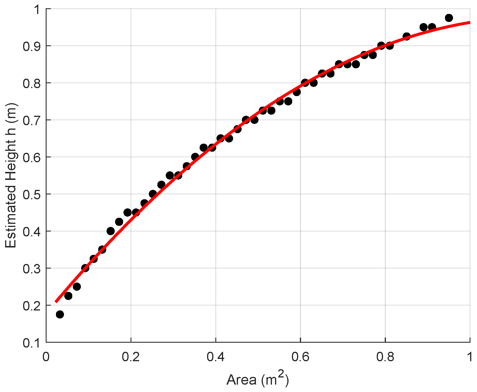
The quadratic regression model fit to predict height is shown in Figure 4. The estimated regression model for height h in terms of area A is:

$$h=-0.5947A^2+1.3802A+0.1774.$$

(11)

The quadratic regression model has a coefficient of determination $R^2$ value of 0.9951. Then the moment of inertia I could be approximated from h given area A.

Although the quadratic regression was originally fitted on a dataset that may contain section combinations that are not fully code-feasible in a strict RC design sense, the subsequent use of this model in the pipeline remains bounded by the same practical limits on member depth and cross-sectional area that were adopted for the case studies. In other words, the regression provides a smooth scaling of area with height within a prescribed range, while the underlying dimensional limits on the sections continue to reflect typical RC practice and prevent extremely unrealistic geometries from entering the analysis.

4.3. RC Material Model and Design Constraints

Topology-optimization constraints guide the algorithm toward practical designs. Equilibrium constraints ensure force and moment balance. Volume constraints limit material usage. Serviceability constraints control deflections and vibrations. In this work, volume fraction (Equation (12)) and area bounds (Equation (13)) are enforced during optimization.

• Volume Reduction: Limit total volume to a fraction of the original full design:

  $${\displaystyle \frac{V_{\mathrm{opt}}}{V_{\mathrm{org}}}}-V_f\le 0.$$

  (12)

  where:
  $V_{\mathrm{opt}}$ is the volume of the optimized structure, computed as the sum of element volumes using optimal cross-sectional areas,
  $V_{\mathrm{org}}$ is the volume of the original fully solid design, computed using the maximum cross-sectional area $A_{\max }$ of the optimization input,
  $V_f$ is the prescribed volume fraction limit.
• Cross-Sectional Area Bounds:

  $$A_{\min }-A_e\le 0\mathrm{and}{A}_e-A_{\max }\le 0.$$

  (13)

  where $A_e$ is the optimal area of element e, and $A_{\min },A_{\max }$ are the lower and upper area bounds.

The combination of a global volume fraction constraint and local area bounds follows common practice in density- and ground-structure-based topology optimization, where minimum feature sizes and manufacturability limits are enforced through volume control and implicit or explicit length scale restrictions [26,33,34]. For RC frames, these bounds also align with constructability constraints on minimum bar spacing and concrete cover mandated by design standards.

In the present work, each frame member is modeled as a transformed reinforced-concrete section so that the contribution of steel reinforcement is captured within an equivalent linear-elastic stiffness representation. The section properties are expressed in terms of the concrete modulus $E_c$, steel modulus $E_s$, reinforcement ratio $r_o$, and modular ratio $n=E_s/E_c$.

A global volume fraction constraint is enforced by penalizing designs whose total optimized volume exceeds a prescribed fraction of the corresponding fully solid ground structure. Element-level axial, shear, and bending stresses, together with derived quantities such as slenderness and Euler buckling load, are evaluated for the optimized layouts and used to interpret the resulting load paths, but they are not treated as active design constraints in the present optimization setup. Detailed code-based checks on steel yielding, concrete cracking, shear capacity, and ultimate compressive strength are therefore reserved for subsequent member-level design verification rather than being enforced during the topology-optimization stage.

4.4. Penalization

The optimization is carried out under a global volume fraction constraint, which is handled by augmenting the compliance objective with a quadratic penalty term. This penalty increases proportionally to the square of the violation of the prescribed volume bound, so that designs whose total optimized volume exceeds the target fraction of the fully solid ground structure are increasingly disfavored.

For a generic constraint measure $g\le 0$, the corresponding quadratic penalty contribution can be written as

$$\mathrm{Penalty}=\left\{\begin{array}{cc}{g}^2,\hfill & \mathrm{if}g>0,\hfill \\ 0,\hfill & \mathrm{otherwise},\hfill \end{array}\right.$$

(14)

where g denotes the difference between the actual value and its allowable limit. In the present work, this structure is applied to the global volume fraction, so that the penalized objective becomes

$$\Pi =\mathrm{Compliance}+\mathrm{penaltyFactor}\times \mathrm{Penalty},$$

(15)

with $\mathrm{Compliance}={\mathbf{u}}^{\top }\mathbf{F}$ and penaltyFactor a large positive scalar that controls the strength of the volume constraint.

Element-level axial, shear, and bending stresses are computed for the optimized frames and used to interpret the internal force paths, but they are not included as active constraints in the current penalized objective.

4.5. Stopping Criteria

Particle Swarm Optimization (PSO) is selected as the optimizer for compliance minimization in this work due to its demonstrated suitability for structural optimization problems with non convex and discontinuous design spaces, as reported, for example, in isogeometric topology optimization and broader engineering applications [35,36,37]. PSO has gained recognition for its simplicity, ease of implementation, and derivative-free nature, making it directly applicable to the non-convex, discrete design space of RC frames without requiring gradient information [35,36].

Convergence is affected by stoppage criteria. The algorithm terminates when either of the following conditions is met:

$$k\ge k_{\max }\mathrm{or}|J^{\left(k\right)}-J^{(k-1)}|<ϵ.$$

(16)

where:

• k: Current iteration number,
• $k_{\max }$: Maximum number of allowed iterations,
• $J^{\left(k\right)}$: Cost function value at iteration k,
• $ϵ$: Specified convergence tolerance.

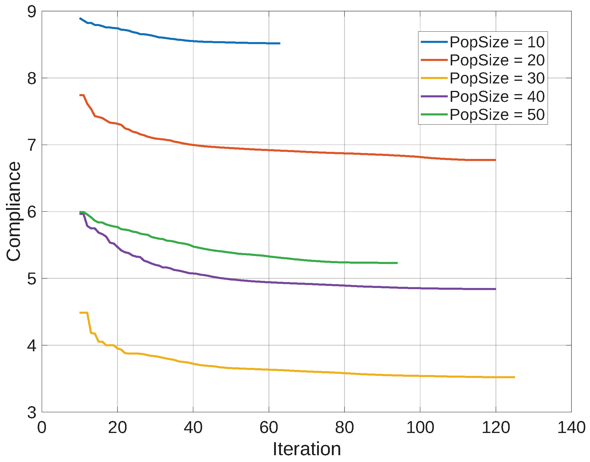
The swarm-based PSO optimizer convergence is broadly affected by the population size as well. The larger the population size, the faster the convergence will be. However, it increases the time elapsed.

4.6. Meshing

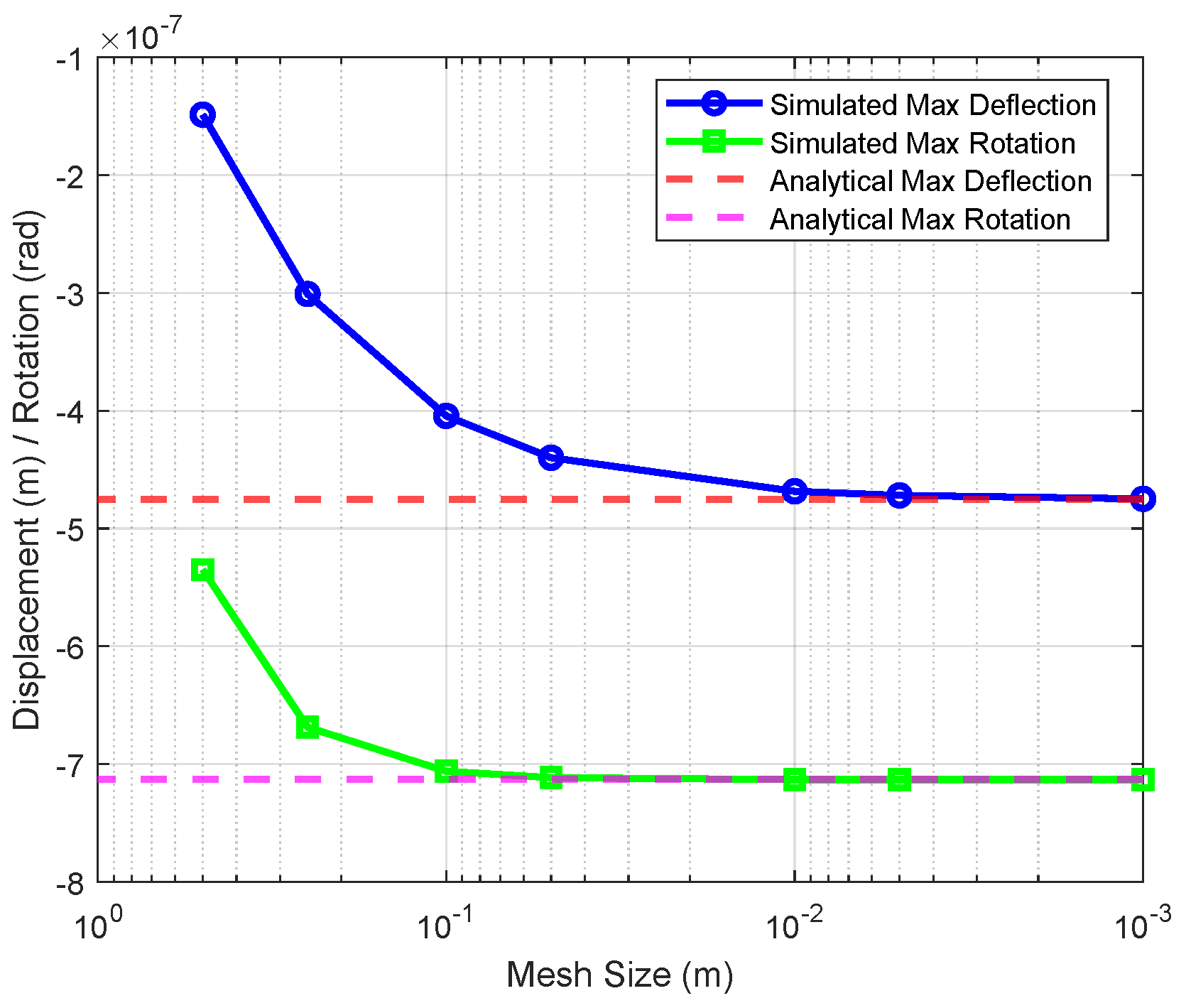
The mesh size convergence plot is shown. The level of fineness can also be taken from the fact that the internal response may not further bring meaningful change in compliance that ultimately leads to change in the size of the design parameters for that element or segment.

Maximum vertical deflection could be computed as:

$${\delta }_{\max }={\displaystyle \frac{P{L}^3}{3EI}}.$$

(17)

where:

• P: Point load,
• L: Length of the beam,
• E: Modulus of elasticity,
• I: Moment of inertia.

Similarly, the maximum rotation ${\theta }_{\max }$ is given by:

$${\theta }_{\max }={\displaystyle \frac{P{L}^2}{2EI}}.$$

(18)

A $1\mathrm{m}$ long cantilever beam under $1\mathrm{kN}$ load was discretized between 50 cm and 1 mm. The corresponding vertical deflection and rotation were recorded at the tip of the beam. The results were compared with those of the corresponding analytical. The normalized difference between the analytical and the simulated values for deflection reaches 7.4% at 5 cm meshing size, while for rotation at 10 cm meshing size it is only 0.93%. While 5 cm spacing is ideal for detailed values, the compliance is not significantly affected within this range as can be seen in

Table 1. Maximum Deflection and Rotation vs. Mesh Size.

Mesh Size (m)	Max Deflection ($\mathsf{\mu }$m)	Max Rotation ($\mathsf{\mu }$rad)
0.5	0.1486	0.5349
0.25	0.3009	0.6687
0.1	0.4044	0.7061
0.05	0.4399	0.7115
0.01	0.4684	0.7132
0.005	0.4719	0.7132
0.001	0.4748	0.7132
Analytical	0.4751	0.7127

. Hence, considering the computational burden, a 10 cm meshing size could be fairly adopted. According to Figure 5, a meshing size between 10 cm and 25 cm could also be a considerable range for topology optimization, especially for preliminary design.

4.7. Matrix Singularity Regularizer and Size Threshold

The Frobenius norm ${\parallel \mathbf{K}\parallel }_F$ provides a scalar measure of a matrix’s total energy by aggregating the squared magnitudes of all its entries $K_{ij}$. This norm is particularly useful in structural analysis, where $\mathbf{K}\in {\mathbb{R}}^{m\times n}$ often represents a global or local stiffness matrix, and each term $K_{ij}$ corresponds to the interaction between degrees of freedom i and j. The threshold $\tau$ defines a lower bound below which the matrix or its components may be considered numerically negligible.

$${\parallel \mathbf{K}\parallel }_F=\sqrt{\sum _{i=1}^m\sum _{j=1}^n{\left|K_{ij}\right|}^2}\le \tau .$$

(19)

It is used for matrix regularization to ensure invertibility when stiffness matrices become ill-conditioned or nearly singular due to very small values during the numerical solution of equilibrium equations.

$${\mathbf{K}}_{\mathrm{reg}}=\mathbf{K}+ϵ·{\parallel \mathbf{K}\parallel }_F·\mathbf{I}.$$

(20)

where:

• ${\mathbf{K}}_{\mathrm{reg}}$: Regularized stiffness matrix,
• $ϵ$: Small regularization factor ${10}^{-10}$,
• $\mathbf{I}$: Identity matrix of the same dimension as $\mathbf{K}$.

This additive term ensures that ${\mathbf{K}}_{\mathrm{reg}}$ becomes positive definite and invertible, enabling stable computation of displacements $\mathbf{u}$ from the equilibrium system.

4.8. Element Removal and Area for the Optimal Frame

Post-optimization processing involves two steps: (i) removing elements with poor mesh quality based on the removal ratio, Equation (21), and (ii) assigning a representative area to each retained element using the mean area of valid sub-elements, Equation (22). This ensures structural reliability and enables consistent comparison across optimized frames.

The idea of post processing optimized layouts by removing poorly resolved or low-density members and assigning representative section properties is consistent with post editing strategies used in density based topology optimization to improve robustness and manufacturability, particularly in the presence of mesh dependent artifacts. Here, the same philosophy is adapted to frame elements through the removal ratio $n_r$ and mean area assignment.

To ensure fairness and consistency in selecting the optimal frame after analysis, the quality of meshed elements is evaluated using relative metrics instead of absolute counts. Relying on a fixed number of sub-elements falling below a minimum area threshold $A_{\min }$ can introduce bias, as elements may contain varying numbers of sub-elements. To address this, the removal ratio $n_r$ is introduced, quantifying the proportion of sub-elements within an element whose areas are less than $A_{\min }$. An element is excluded from further consideration if $n_r$ exceeds a specified threshold, indicating insufficient mesh quality.

$$n_r={\displaystyle \frac{n_{\mathrm{violating}}}{n_{\mathrm{total}}}}.$$

(21)

where:

• $n_{\mathrm{violating}}$: Number of meshed sub-elements within the parent element area less than $A_{\min }$,
• $n_{\mathrm{total}}$: Total number of meshed sub-elements within the element,
• $n_r$: Removal ratio.

In an effort to assign a uniform area to each element, while assigning the maximum area guarantees safety by accounting for the worst-case requirement, it may lead to overly conservative and uneconomical designs. A more balanced and cost-effective approach involves using the mean area of valid meshed sub-elements, those not filtered out by the removal ratio criterion. This supports both structural performance and material efficiency. In this work, the mean is preferred, and the representative area for each element is computed as:

$$A_{\mathrm{elem}}={\displaystyle \frac{1}{n}}{\displaystyle \sum _{i=1}^n}{A}_i.$$

(22)

where:

• $A_{\mathrm{elem}}$: Assigned uniform area of the element,
• $A_i$: Area of the i-th meshed sub-element that satisfies the minimum area condition,
• n: Number of such valid sub-elements used in the averaging process.

It is important to note that in structural systems such as building frames designed to support slabs, beam elements are typically subjected to distributed gravity loads, and due to their structural function, they may be exempted from the element removal criteria. These frames prioritize continuity and vertical load transfer, making the removal of elements potentially unrealistic.

4.9. Optimal Frame Validation

Elements contributing minimally to stiffness—often artifacts of numerical regularization—are excluded to produce cleaner, manufacturable designs. The pruned frame is reanalyzed under identical loading to validate stiffness retention.

Validation compares two metrics: volume change and compliance increase Equation (25). Excessive volume increase indicates over-compensation for stiffness loss. Large compliance increase signals degraded structural performance.

$$C_{\mathrm{norm}}={\displaystyle \frac{C}{{\parallel F\parallel }^2}}.$$

(23)

where:

• C: Original compliance before optimization,
• ${\parallel F\parallel }^2$: Squared norm of the original load vector,
• $C_{\mathrm{norm}}$: Normalized original compliance.

$$C_{\mathrm{opt},\mathrm{norm}}={\displaystyle \frac{C_{\mathrm{opt}}}{{\parallel F_{\mathrm{filtered}}\parallel }^2}}.$$

(24)

where:

• $C_{\mathrm{opt}}$: Compliance after reanalysis of the filtered optimized frame,
• ${\parallel F_{\mathrm{filtered}}\parallel }^2$: Squared norm of the filtered load vector,
• $C_{\mathrm{opt},\mathrm{norm}}$: Normalized optimized compliance.

Post-optimization reanalysis naturally increases compliance as element removal leads to stiffness loss, a well-documented phenomenon in structural topology optimization (both density- and ground-structure-based). In practice, pruning very low-density or low-area members typically causes a modest rise in compliance on the order of 5–15%, while larger increases (above about 20%) are generally taken to indicate that the pruning has significantly altered the optimal load paths, as reported in recent post-editing and robustness studies for topology-optimized lattices and continua [26,33,34].

For reinforced-concrete frames specifically, a 20% $C_v$ tolerance is reasonable because members are physically bounded by constructability requirements such as aggregate flow and rebar clearance, which preclude the infinitesimal member sizes often allowed in steel topology optimization. In addition, the mandatory retention of floor beams to ensure slab support introduces small compliance penalties that are secondary to detailing feasibility and structural continuity [30]. Within this framework, a $C_v\le 5\%$ threshold identifies very conservative layouts that retain near-original stiffness, while $C_v\le 20\%$ marks high-efficiency solutions that remain compatible with practical RC detailing and frame behavior [38].

$$C_v={\displaystyle \frac{C_{\mathrm{opt},\mathrm{norm}}-C_{\mathrm{norm}}}{C_{\mathrm{norm}}}}.$$

(25)

where:

• $C_{\mathrm{norm}}$: Normalized original compliance,
• $C_{\mathrm{opt},\mathrm{norm}}$: Normalized optimized compliance,
• $C_v$: Compliance-validation metric (relative change).

In practice, the most pronounced validation failures correspond to frames where removal of a column supporting an edge or corner beam produces a large increase in the validation metric $C_v$. For such cases, the removal ratio $n_r$ threshold is first tightened to preserve critical vertical load paths; if this does not restore $C_v$ to the acceptable range, the volume fraction limit $V_f$ for that frame is locally relaxed, trading a modest increase in material usage for a substantial gain in stiffness and robustness.

4.10. Reanalysis, Stress Evaluation, and Compliance Validation

After topology optimization and member pruning, a reduced meshed frame is reconstructed that contains only the active members, and a second finite-element analysis is performed using the same transformed-section model and boundary conditions as in the original ground structure. The resulting displacement field is used to compute both axial and bending stresses in each element, from which a maximum combined stress measure is obtained to visualize the stress distribution and to assess whether the optimized layout remains within the intended elastic range. At the same time, the global compliance of this filtered frame is recomputed and normalized with respect to the filtered load vector, yielding $C_{\mathrm{opt},\mathrm{norm}}$, which is compared to the normalized original compliance $C_{\mathrm{norm}}$ through the validation metric $C_v$. This post-optimization reanalysis quantifies the stiffness loss associated with element removal, highlights cases where column removal significantly alters critical load paths, and complements the volume constraint by providing an explicit stiffness-based acceptance criterion for the RC frame designs.

5. Surrogate Model for Compliance Prediction

5.1. Latin Hypercube Sampling

LHS was used to efficiently select a representative subset of frame structures from a large design space, ensuring broad coverage of the input domain with reduced computational cost [5]. In structural reliability and safety assessment, Latin hypercube sampling has long been used to achieve efficient coverage of high dimensional input spaces while maintaining accuracy in tail events and extreme responses. By adopting LHS for frame sampling in the present context, we leverage the same rationale—namely, that a relatively small but carefully stratified set of evaluations can yield reliable information about global performance trends.

Parameters included both geometric and topological attributes relevant to frame design, such as nodal coordinates, member connectivity, number of stories and bays, bay width, and story height. Higher-level features like inclined columns, connectivity level, and structural cluster membership were also considered. Each parameter range was divided into equal intervals, with one value sampled per interval and sampling orders permuted to avoid inter-variable correlation. The full parameter set is:

$$\begin{array}{cc}\hfill P=& \{\mathrm{Bay}\mathrm{Width},\mathrm{Story}\mathrm{Height},\mathrm{Number}\mathrm{of}\mathrm{Bays},\hfill \\ \hfill & \mathrm{Number}\mathrm{of}\mathrm{Stories},\mathrm{Nodes}\mathrm{Matrix},\mathrm{Connectivity}\mathrm{Matrix}\}.\hfill \end{array}$$

(26)

Original ground structures and their perturbed variants were both included, ensuring diversity and representativeness across categories.

5.2. Graph-Based Approach

An alternative to vectorizing raw nodal coordinates is to represent each structure as a graph, enabling feature extraction aligned with graph neural network (GNN) applications. This approach captures both topological and geometric properties using a compact set of descriptors [8,39]. In the first step, we use a base feature vector

$$\begin{array}{cc}\hfill F=& \{\mathrm{Number}\mathrm{of}\mathrm{Nodes},\mathrm{Number}\mathrm{of}\mathrm{Edges},\mathrm{Average}\mathrm{Degree},\mathrm{Maximum}\mathrm{Degree},\hfill \\ \hfill & \mathrm{Graph}\mathrm{Diameter},\mathrm{Average}\mathrm{Betweenness}\mathrm{Centrality},\mathrm{Mean}\mathrm{Edge}\mathrm{Length},\hfill \\ \hfill & \mathrm{Edge}\mathrm{Length}\mathrm{Std}.\mathrm{Dev}.,\mathrm{Bounding}\mathrm{Box}\mathrm{Volume},\mathrm{Graph}\mathrm{Density},\hfill \\ \hfill & \mathrm{Number}\mathrm{of}\mathrm{Storeys}\},\hfill \end{array}$$

(27)

which already encodes basic size, connectivity, and geometric scale of each framed structure.

To better capture structural load flow and redundancy, we extend this representation with graph features that are sensitive to dominant paths and alternative routes. Specifically, we augment F to an extended feature vector

$$\begin{array}{cc}\hfill F^{\mathrm{ext}}=& F\cup \{\mathrm{Maximum}\mathrm{Betweenness}\mathrm{Centrality},\mathrm{Betweenness}\mathrm{Centrality}\mathrm{Std}.\mathrm{Dev}.,\hfill \\ \hfill & \mathrm{Backbone}\mathrm{Ratio},c_{\mathrm{backbone}},\mathrm{Cyclomatic}\mathrm{Number}\},\hfill \end{array}$$

(28)

where the maximum and standard deviation of betweenness centrality highlight highly loaded joints and the spread of flow concentration, the backbone ratio and $c_{\mathrm{backbone}}$ quantify the size and connectivity of the 2-core size that carries most of the load, and the cyclomatic number measures the number of independent cycles, providing an indicator of load-path redundancy. These additional descriptors emphasize how forces can redistribute within the frame and therefore provide a richer structural signal for subsequent learning and optimization.

This construction follows the insight that graph invariants, such as degree distributions, diameters, and betweenness based measures, encode structural flow and redundancy in a way that is robust to local geometric variations. Comparable graph descriptors and latent representations have also proved effective in recent work on generative modeling and optimization of truss meta-materials, supporting their use here as compact yet expressive structural features for RC frame candidates.

5.3. Gaussian Process Surrogate Model

A sparse Gaussian Process surrogate is trained on LHS-sampled frames with FEM-computed compliance. The model then predicts compliance for unevaluated frames, enabling rapid candidate ranking without exhaustive simulation.

The surrogate model predicts compliance directly, bypassing the need for nodal displacement and FEM-based compliance calculations.

A sparse GP approximation, in which only $m\ll n$ representative inducing points are used, reduces the computational complexity from $\mathcal{O}\left(n^3\right)$ for a full GP to $\mathcal{O}\left(n{m}^2\right)$, making it tractable for the large frame populations considered in this work.

5.3.1. Sparse Gaussian Process

The sparse GP is defined as:

$$\begin{array}{c}\hfill f\left(x\right)\sim \mathcal{GP}\left(m\left(x\right),\tilde{k}(x,x^{\prime })\right).\end{array}$$

(29)

where:

• $m\left(x\right)=\mathbb{E}\left[f\right(x\left)\right]$: Mean function, expected value of the function at input x,
• $\tilde{k}(x,x^{\prime })$: Approximate covariance function defined using inducing points.

The approximate kernel $\tilde{k}(x,x^{\prime })$ is computed as:

$$\begin{array}{c}\hfill \tilde{k}(x,x^{\prime })=k_{xZ}{K}_{ZZ}^{-1}{k}_{Z{x}^{\prime }}.\end{array}$$

(30)

where:

• $k_{xZ}$: Covariance vector between input x and the inducing points Z,
• $K_{ZZ}$: Covariance matrix between the inducing points,
• $k_{Z{x}^{\prime }}$: Covariance vector between inducing points and input $x^{\prime }$.

5.3.2. Radial Basis Function Kernel

The RBF kernel used to define the covariance terms is given by:

$$\begin{array}{c}\hfill k(x,x^{\prime })={\sigma }^2\exp \left(-{\displaystyle \frac{\parallel x-x^{\prime }{\parallel }^2}{2l^2}}\right).\end{array}$$

(31)

where:

• ${\sigma }^2$: Variance parameter (scale of the kernel),
• l: Length-scale parameter, controlling the smoothness,
• $\parallel x-x^{\prime }{\parallel }^2$: Squared Euclidean distance between input vectors x and $x^{\prime }$.

5.3.3. Automatic Relevance Determination

Automatic Relevance Determination (ARD) is a Bayesian feature–weighting approach in which each input dimension is associated with its own hyperparameter (for example, a length scale in the covariance function), allowing the model to infer the importance of each covariate directly from the data. Dimensions that are informative for predicting the target are assigned small length scales, so the latent function can vary rapidly along those directions, whereas uninformative inputs receive very large length scales, effectively flattening the response and pruning those dimensions from the model. This leads to sparse, interpretable representations and often better generalization in high–dimensional settings where many candidate descriptors are only weakly relevant [40].

A common choice is the squared exponential ARD kernel

$$k_{\mathrm{ARD}}(\mathbf{x},{\mathbf{x}}^{\prime })={\sigma }_f^2\exp \left(-{\displaystyle \frac{1}{2}}{\displaystyle \sum _{d=1}^D}{\displaystyle \frac{{(x_d-x_d^{\prime })}^2}{{\mathcal{l}}_d^2}}\right),$$

(32)

where ${\sigma }_f^2$ is the signal variance and ${\mathcal{l}}_d$ is the ARD length–scale associated with input dimension d.

5.4. Top-k Ranking on the Validation Pool

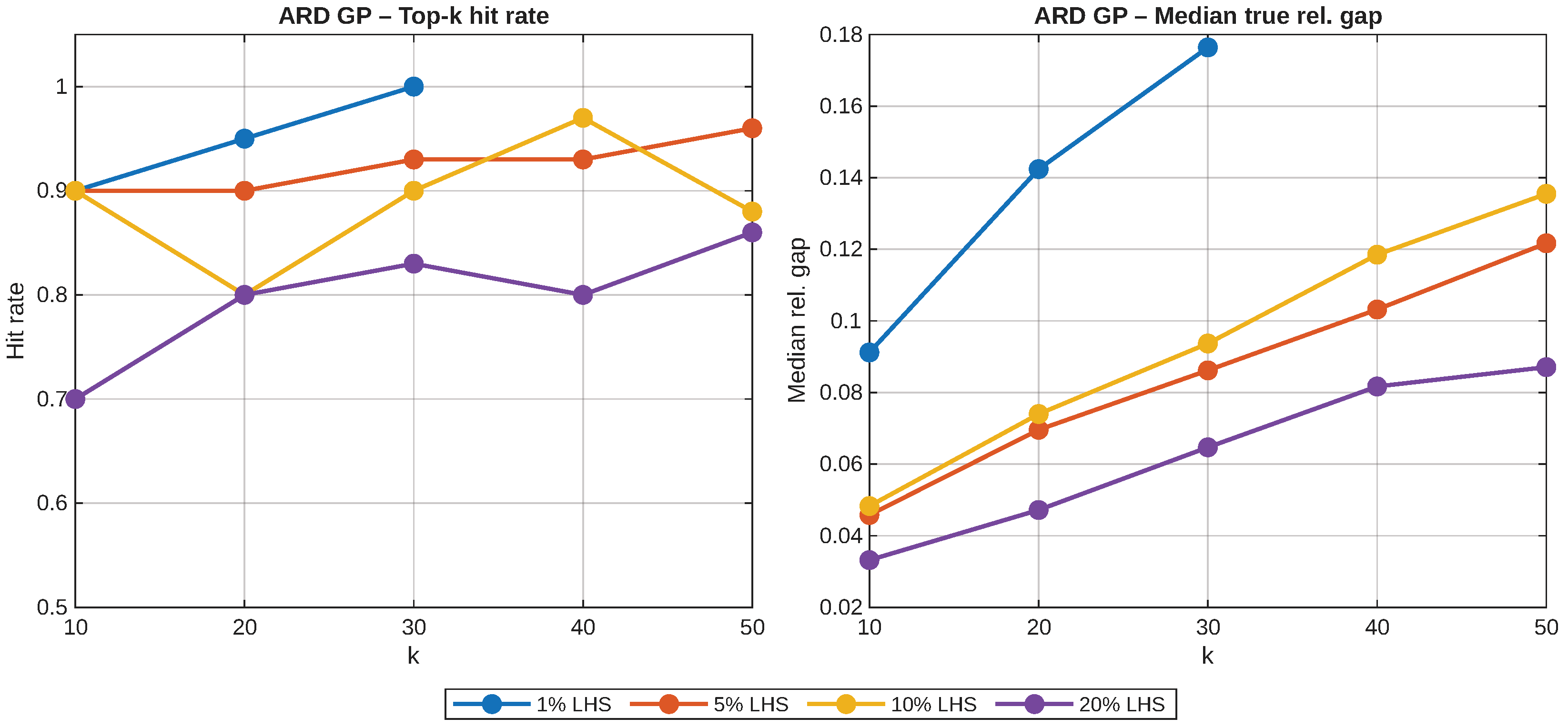
We evaluate the ranking quality of the surrogate models on a fixed $10\%$ validation pool by analyzing how well they retrieve near-optimal designs within a shortlist of size k. For each validation frame, the surrogate produces a ranking of all candidate designs according to the predicted compliance. A top-k hit occurs if the true best design (i.e., the frame with minimal FE-computed compliance) appears anywhere among the k highest-ranked candidates. Varying k (e.g., $k=10,20$) allows us to quantify how large a shortlist is required for the surrogate to reliably include the globally optimal frame.

On this basis, we report two metrics as functions of k. The hit rate at k is the fraction of validation frames for which the minimal FE-computed design is contained in the top-k list:

$$\mathrm{Hit}\mathrm{rate}\left(k\right)={\displaystyle \frac{1}{N_{\mathrm{val}}}}{\displaystyle \sum _{i=1}^{N_{\mathrm{val}}}}\mathbb{I}\left(y_i\in {\mathcal{R}}_k^{\left(i\right)}\right),$$

(33)

where:

• $N_{\mathrm{val}}$: Number of validation instances,
• $y_i$: Index of the minimal FE-computed design for instance i,
• ${\mathcal{R}}_k^{\left(i\right)}$: Set of the k top-ranked candidates according to the surrogate for instance i,
• $\mathbb{I}(·)$: Indicator function, equal to 1 if the condition is satisfied and 0 otherwise.

Complementarily, the median true relative gap at k measures how close the best design found within the top-k list is to the true optimum in terms of compliance. Let $f_i^{★}$ be the minimal compliance for validation instance i and let ${\widehat{f}}_i^{\left(k\right)}$ be the smallest compliance among the k designs in ${\mathcal{R}}_k^{\left(i\right)}$. We define

$$\mathrm{Median}\mathrm{true}\mathrm{rel}.\mathrm{gap}\left(k\right)={\mathrm{median}}_{i=1,\dots ,N_{\mathrm{val}}}\left({\displaystyle \frac{{\widehat{f}}_i^{\left(k\right)}-f_i^{★}}{f_i^{★}}}\right).$$

(34)

Small values of $\mathrm{Median}\mathrm{true}\mathrm{rel}.\mathrm{gap}\left(k\right)$ indicate that, even when the exact optimum is not always ranked first, the shortlisted designs in the top-k set remain close to the global optimum in terms of structural performance.

In the context of this work, high hit rates at modest shortlist sizes (e.g., k = 10 or 20) and small median relative gaps indicate that the surrogate reliably surfaces near optimal frames without requiring exhaustive FEM evaluation of the full population. This directly addresses the requirement that sampling and surrogate modeling be judged by their impact on final ranking quality near the optimum, rather than by aggregate regression metrics alone, as emphasized in reliability oriented sampling studies.

In the present validation, the reference optimum $f_i^{★}$ for each instance is defined as the best FEM-evaluated candidate within the corresponding validation pool, rather than the global optimum over the entire enumerated population, which would be computationally prohibitive to evaluate exhaustively. Accordingly, the hit-rate metric and the median true relative gap quantify how reliably the surrogate recovers near-best designs among the FE-evaluated candidates, not an absolute global optimum over all generated frames.

The graph-based LHS and sparse GP framework implemented here follows the rationale established in structural reliability and safety assessment [5,6,7,8], where sampling strategies are judged not only by nominal design-space coverage but also by their ability to identify near-optimal or critical designs with minimal FE evaluations. This is analogous to adaptive substructure identification [20] and ML–FE mesh optimization for ground settlement prediction [21], where surrogate models filter large candidate sets before full-scale simulation. In those applications, as in the present pipeline, the surrogate’s primary value lies in enabling design-space filtering under computational constraints rather than replacing high-fidelity analysis entirely. The top-k ranking metrics (hit rate and median relative gap, Section 6.3.3) directly address the concern that sampling and surrogate performance must be assessed in terms of final design reliability near the optimum, not only regression accuracy over the full population.

6. Case Study: Optimal Ground-Structure-Based Reinforced-Concrete Frame Optimization

In this section, the building domain of width-to-height aspect ratios of 1:1 and 1:1.5 is examined under gravity loading. The candidate frames could vary in both the number of stories and the bay, in addition to the width and height of the bay. Hence, the number of top nodes could also vary for the sake of fairness; the same amount of gravity loading is shared among the top nodes of each frame at the non-iterative compliance computation and prediction stage. Volume constraints are considered for the optimization.

Gravity loads are applied as equal downward nodal forces distributed among all non-base nodes to simulate floor-level loading at every story, and a notional lateral load is applied at the topmost left node to account for geometric imperfection effects per [27]. All base nodes are fully fixed, restraining translational and rotational degrees of freedom.

These loading conditions are intentionally simplified and are selected to exercise the stiffness-driven response of the candidate frames under combined gravity and a notional lateral disturbance, rather than to represent a complete set of RC building design actions. Realistic design would require combinations of gravity, wind, and seismic loads with appropriate load factors, serviceability drift limits (e.g., story drift < H/400 per [27]), second-order (P–$\Delta$) effects, accidental eccentricities, column slenderness checks, and detailed joint and shear demands, none of which are modeled in the present case studies. Accordingly, the optimized frames should be viewed as illustrative stiffness-screening examples under idealized loading, and any code-compliant design for a specific structure would need a subsequent multi-load-case verification in line with RC frame design standards.

The PSO optimizer is used in the final stage of this pipeline: that is, in the size optimization of systematically selected candidate topologically optimal frames. The PSO parameters shown in

Table 2. PSO Parameters and Values used.

Parameter	Value
Population size	10–50
Maximum iteration	200
Inertia weight	0.5
Cognitive coefficient	1.5
Social coefficient	1.5
No. of Runs	10

are kept the same across all considered frames.

6.1. Implementation Verification

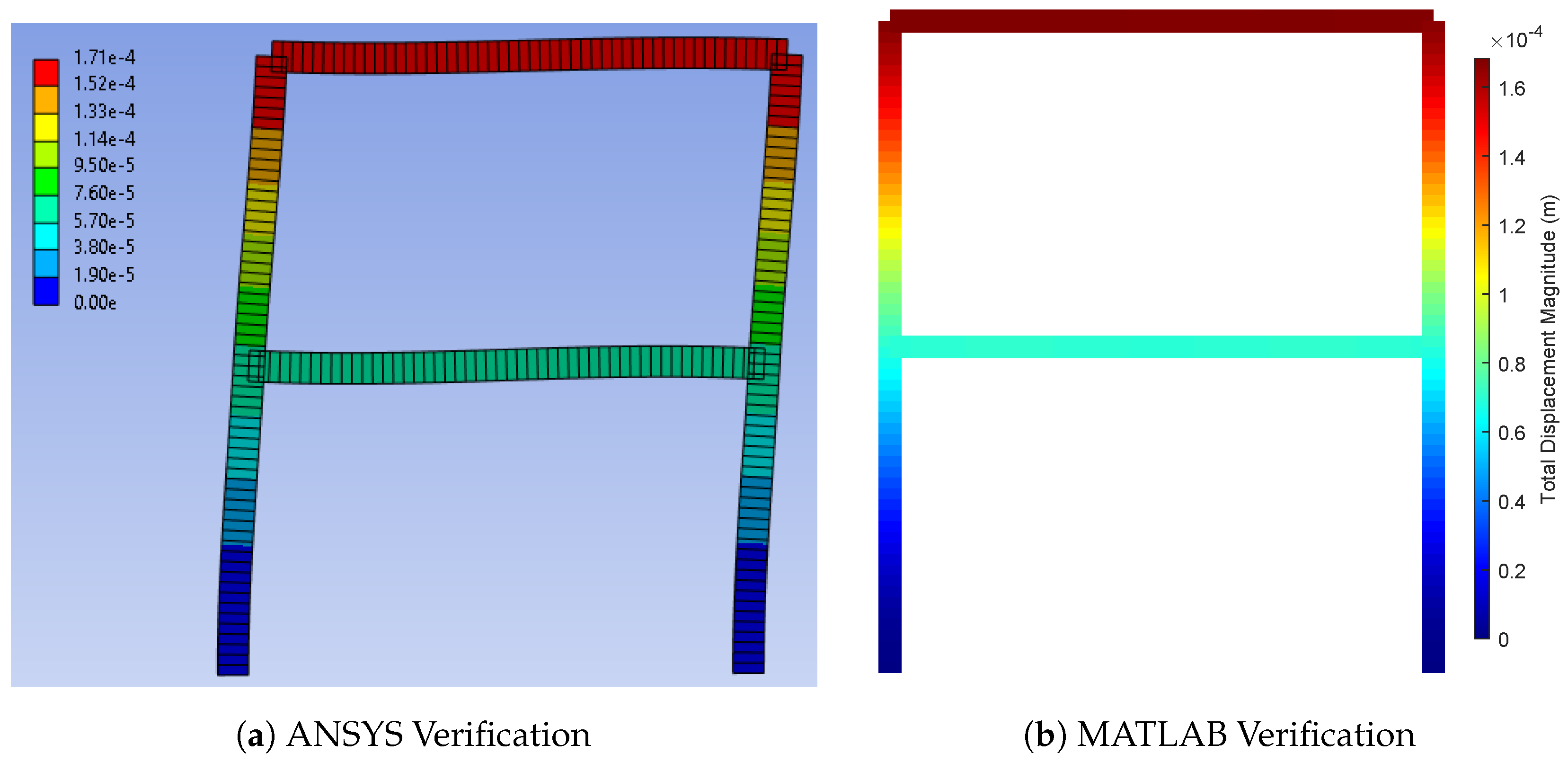
The FEM implementation is developed in Matlab (version 2023), and verification of the computational script is essential to ensure its accuracy and reliability. For this purpose, a one-bay, two-story frame consisting of six elements was modeled and analyzed using both the Matlab code and a commercial FEM software, ANSYS (version 2023 R1). Models of the same frame were created, meshed, and subjected to various loading conditions, including lateral point loads, distributed gravity loads, and gravity point loads. The cross-sectional properties, mesh sizes, applied loads, and resulting internal responses such as stresses and displacements were recorded. A comparative analysis of the stresses and deflections obtained from Matlab and ANSYS was performed to evaluate similarities and differences between the two solutions.

It is important to note that the primary objective of the Matlab script is to accurately predict displacements, particularly lateral deflections. While stress results from Matlab and ANSYS are compared, some discrepancies are expected due to differences in modeling assumptions and the level of detail considered by the two FEM approaches. For example, the Matlab script may not include all the structural components or effects taken into account by ANSYS. Despite these differences, close agreement in displacement results verifies the effectiveness of the Matlab implementation for its intended purpose. This level of agreement is consistent with previous verification studies comparing in house topology-optimization codes against commercial FE software for frame and continuum benchmarks, and is considered sufficient for the present role of the FE solver as a compliance evaluator within the broader pipeline.

A 1 kN point load is applied horizontally to the right at the top left node Figure 6. A square cross section with a side length of 30 cm is used. According to MATLAB, the maximum total deformation is 1.68 × 10⁻⁴, which closely matches the result obtained from ANSYS which is 1.71 × 10⁻⁴.

The PSO parameters are kept fixed across all candidate frames to enable a consistent comparison of topologies; however, this also means that the reported designs reflect one particular configuration of a stochastic optimizer rather than a fully tuned algorithmic setting. For a subset of representative frames, multiple PSO runs with different random seeds produced different best compliances and area distributions, indicating run-to-run variability typical of metaheuristic search.

The PSO parameters are kept fixed across all candidate frames to enable a consistent comparison of topologies; however, this also means that the reported designs reflect one particular configuration of a stochastic optimizer rather than a fully tuned algorithmic setting. For a subset of representative frames (Frame 24 and Frame 5464 in Section 6.3.7), multiple PSO runs with different random seeds produced different best compliances and area distributions, indicating run-to-run variability typical of metaheuristic search. Future work should explore sensitivity to PSO initialization, comparison with alternative gradient-based optimizers, and hybrid approaches that combine global PSO search with local gradient refinement.

6.2. Effect of Nodal Location Interval

To investigate the effect of nodal location intervals, different combinations of spacing along the x- and y-axes were tested: $(0.2,0.2)$, $(0.2,0.5)$, and $(0.5,0.2)$. A domain with an aspect ratio of 1:1, which is presented in Section 6.3, is considered.

The first pair $(0.2,0.2)$ results in a significantly large number of computational frames, making it computationally expensive. Due to the small interval, a slightly larger spacing may be more efficient.

The second and third combinations, $(0.2,0.5)$ and $(0.5,0.2)$, yield a comparatively similar number of frames, both of which are more manageable.

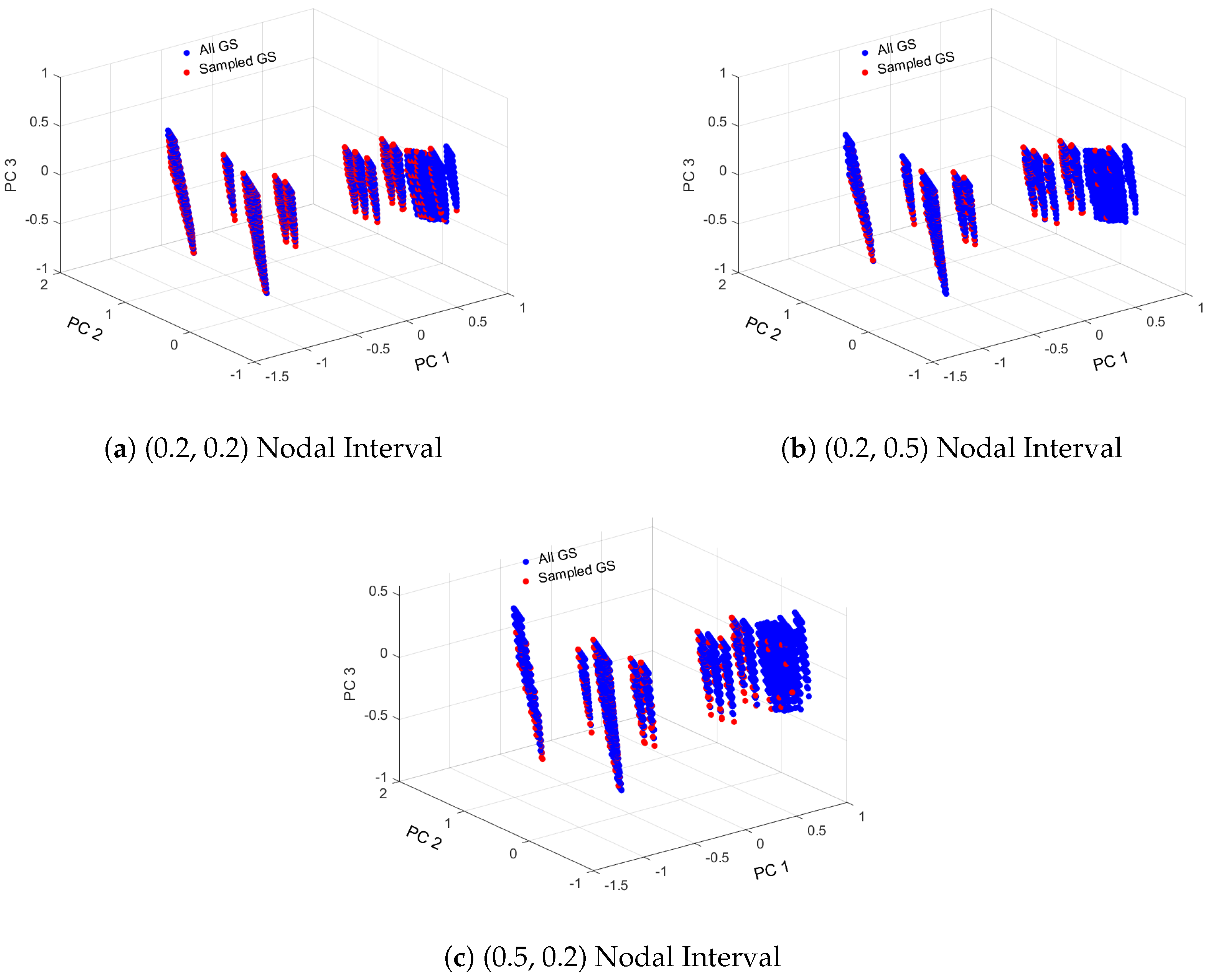
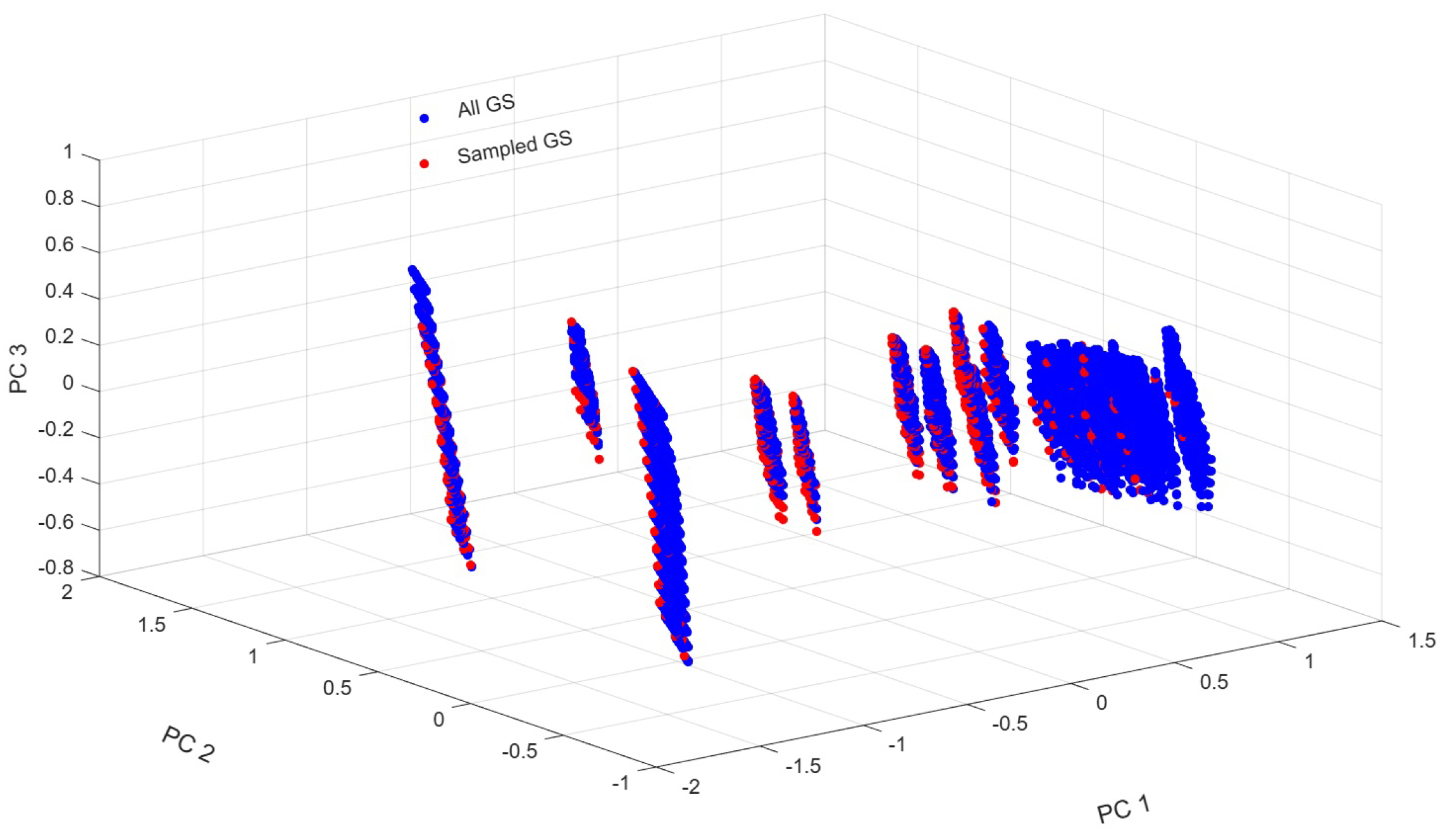
For each of the three interval configurations, a graph-based LHS scattered plot was generated to visualize the distribution of nodal locations.

The clusters are almost similar across the plots. The PC3 axis of Figure 7c, reduced to 0.5, could be taken as a small reduction in the identification of the samples. Hence, Figure 7b could be chosen in this case.

The second and third nodal location intervals were compared: the second produced 446 unique samples with sampling 2%, resulting in RMSE = 2.0696, MAE = 1.2473, and $R^2$ = 0.9842; The third yielded 409 unique samples with the same sampling rate 2%, achieving RMSE = 1.8961, MAE = 1.1727, and $R^2$ = 0.9887. While the third one shows slightly better model performance, the second benefits from a relatively greater number of samples. For a $1:1$ domain, both approaches could be considered equivalent. However, the second one is selected to take advantage of the larger dataset for potentially better generalization. Results for different aspect ratios may vary from what is found here.

6.3. Frame with 1:1 Aspect Ratio

Width of 10m and height of 10 m domain is used. Bay width bound of [3 m, 7 m] and story height bound of [2.8 m, 4 m] are set. Nodal location is allowed to be generated with an interval of 0.2 m along both axes. This generated 26,208 basic ground structures and a total of 438,984 ground structures when perturbation is considered as shown in Figure 8. Though the level of connectivity could differ, for any of those Level 1, Level 2, or fully connected levels, the total number of GS remains the same. Perturbation of 0.2 m is used. Though Level 1 and fully connected levels were considered, the optimization mainly focused on the Level 2 connectivity, where each node is allowed to become connected to its next node beyond the immediate neighbor node. This could be taken as an intermediate connectivity between level one and fully connected connectivities, thereby excluding potentially slender elements. The computational load is further reduced by increasing the nodal location interval along the elevation to 0.5 m. Accordingly, the total number of GS reduces to 63,784.

6.3.1. Effect of Sampling Ratio

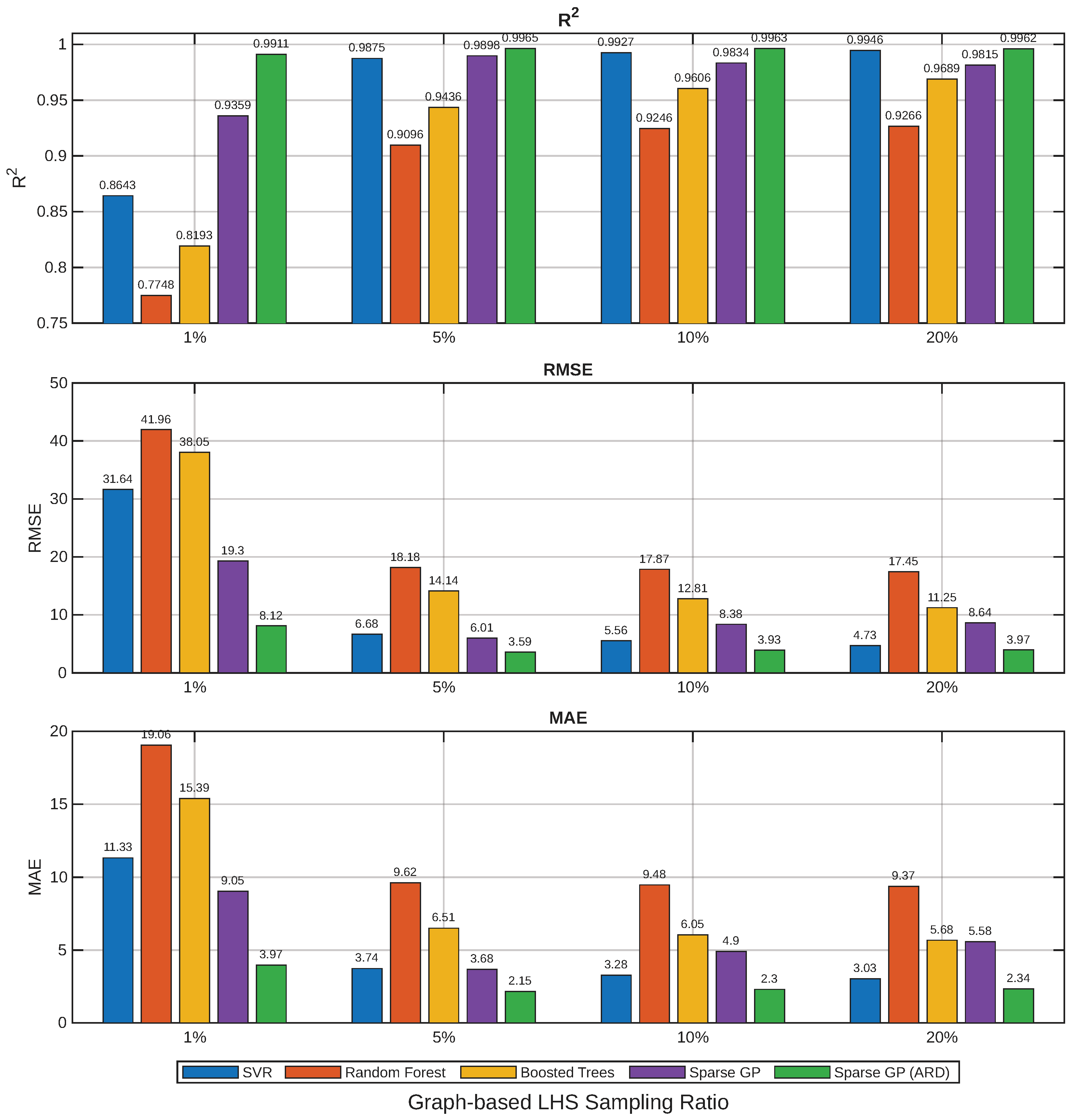
The amount of data used to train the surrogate models influences their predictive performance by varying the graph-based Latin hypercube sampling (LHS) ratio, which is investigated. Specifically, LHS subsets corresponding to $1\%$, $5\%$, $10\%$, and $20\%$ of the full generated dataset are constructed, and separate surrogate models are trained on each subset. For each sampling ratio, we evaluate several regression models and compare their performance in terms of $R^2$, mean absolute error (MAE), and root mean squared error (RMSE) on a held-out validation set. It was demonstrated on the first case study frame with a 1:1 aspect ratio presented below. Across these experiments, sparse Gaussian processes (sparse GP) and automatic-relevance-determination Gaussian processes (ARD GP) consistently emerge as the best-performing models.

6.3.2. Performance of Multiple Models

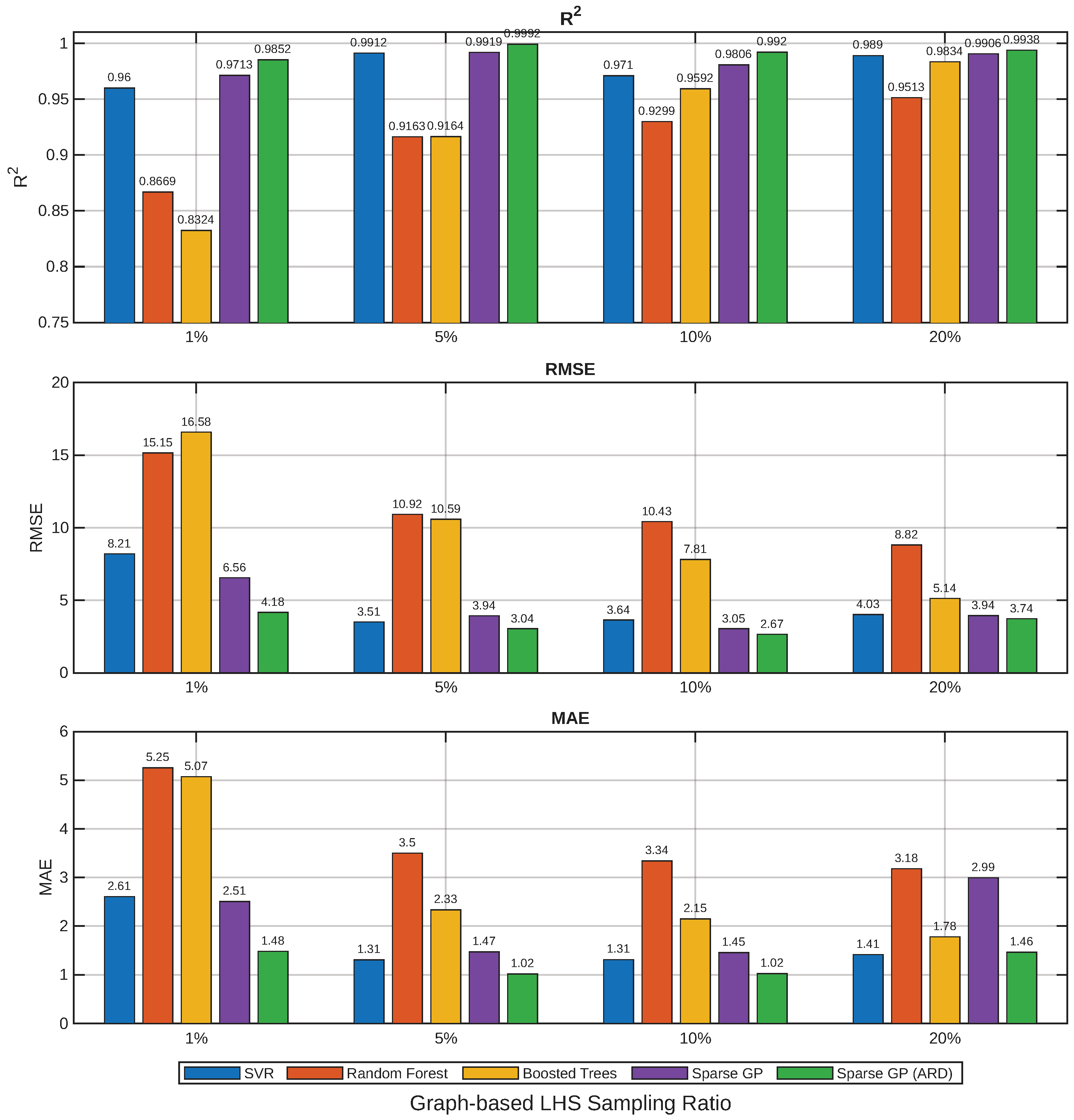
Apart from sparse GP and sparse GP ARD, support vector machine (SVM), random forest (RF), and gradient boost (GB) models were used and compared. In multiple cases, the sparse GP could be preferable. For the $(0.2,0.5)$ nodal interval range discussed above, the performance of these models is summarized on Figure 9.

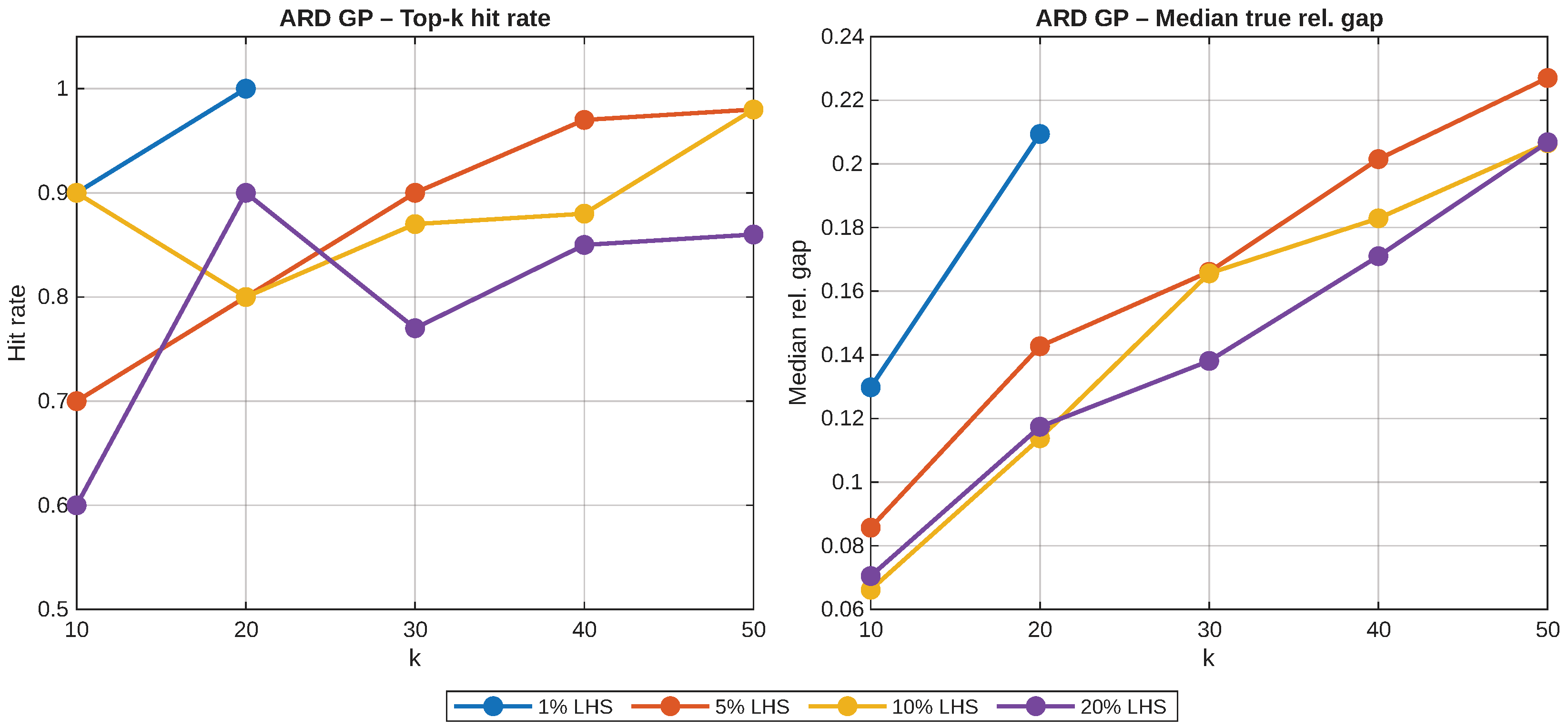
Different graph-based LHS sampling ratio sensitivity is recorded. $1\%$ sampling least performance given the fact that the sampling is smaller. The $5\%$ sampling has the best performance. When observed in association with the near-optimal performance evaluation in terms of the metrics reported on Figure 10, the hit rate score of $10\%$ sampling, which is $0.9$, is the highest at the top $k=10$ optimal frames and smallest median true relative gap of $0.066$. Within the selected $10\%$ sampling, the sparse GP (ARD) showed the best performance, and accordingly, the model is preferred across all the case studies.

These findings are based on representative realizations for the investigated aspect-ratio domains and connectivity settings and indicate that, under these conditions, a 10% sampling ratio offers a favorable balance between regression accuracy and top-k ranking quality. We emphasize that this should not be interpreted as a universal rule: a single Latin Hypercube realization per configuration cannot fully characterize sensitivity to sampling seeds, alternative connectivities, or additional frame domains. For instance, different random LHS seeds for the same ground-structure population could yield different surrogate prediction maps, and the optimal sampling ratio may vary when extended to aspect ratios beyond 1:1 and 1:1.5 or to connectivity levels beyond Level 2. In practice, the sampling ratio should be treated as a tunable algorithmic parameter whose robustness with respect to random seeds, alternative connectivity patterns, and problem settings warrants further systematic study, potentially through repeated LHS draws and cross-validation across multiple domain configurations.

6.3.3. Top-k Ranking on the Validation Pool

To assess how well the selected surrogates retrieve near-optimal designs, the sparse GP with ARD was selected based on the performance on Figure 9 is further examined using top-k ranking metrics on a fixed $10\%$ validation pool. For each frame in the validation set, the surrogate model produces a ranking of all candidate designs according to the predicted compliance. For a given shortlist size k (here $k\in \{10,20,30,40,50\}$), we record (i) the hit rate at k, defined as the fraction of validation frames for which the minimal FE-computed globally optimal design appears among the top-k candidates, and (ii) the median true relative gap at k, which measures how close the best design found within the top-k list is to the minimal FE-computed. These metrics allow a direct comparison of sparse GP and ARD GP in terms of their ability to surface near-optimal frames within practically sized candidate lists.

6.3.4. Graph-Based LHS Sampling

The graph-based LHS considers important features that could dictate load flow along the frames. This method usually returns multiple same frames to be important or strong neighbors. Hence, the graph-based LHS approach needs to be filtered once sampling is carried out to return unique frames. One may otherwise consider those repeated frames and their frequency as the importance indicator of those frames to be included as samples or even directly as final candidate frames that might be considered for the intended actual topology optimization at the end of this procedure.

Although the number of samples depends on the number of variables or features, a sampling of consistently 10% is used. 1407 unique LHS samples returned. Figure 11 shows how the sampled frames are representative of the population after reducing the dimensionality of the principal component analysis (PCA). The clusters are usually influenced by the number of bays, the number of stories, and their widths and heights. In addition, the layers within each cluster represent frames varied with bay width and story height.

6.3.5. Sparse Gaussian Process Based Compliance Prediction and Candidate Frame Selection

Compliance is computed using elastic FE analysis with transformed-section material properties and a consistent 0.2 m mesh size. A total of 10 kN gravity load is distributed equally among all top nodes. For each frame, a uniform area of elements is used. However, to maintain the same volume of material for each frame, the area of each frame is computed by equating it to the volume of the first frame. The area for the first frame could be reasonably given by:

$$A_{f_{i+1}}={\displaystyle \frac{V_{f_1}}{L_{f_{i+1}}}},i=1,\dots ,n-1.$$

(35)

where:

• $A_{f_{i+1}}$ is the area of frame $i+1$,
• $V_{f_1}$ is the volume of frame 1,
• $L_{f_{i+1}}$ is the total length of the elements of the frame $i+1$,
• n is the number of samples.

Therefore, this compliance does not involve any iteration, optimization, or penalization. Its main objective is to roughly estimate the compliance or stiffness of each frame given relatively the same scenario. The computed values are scaled to 100 for common visualization.

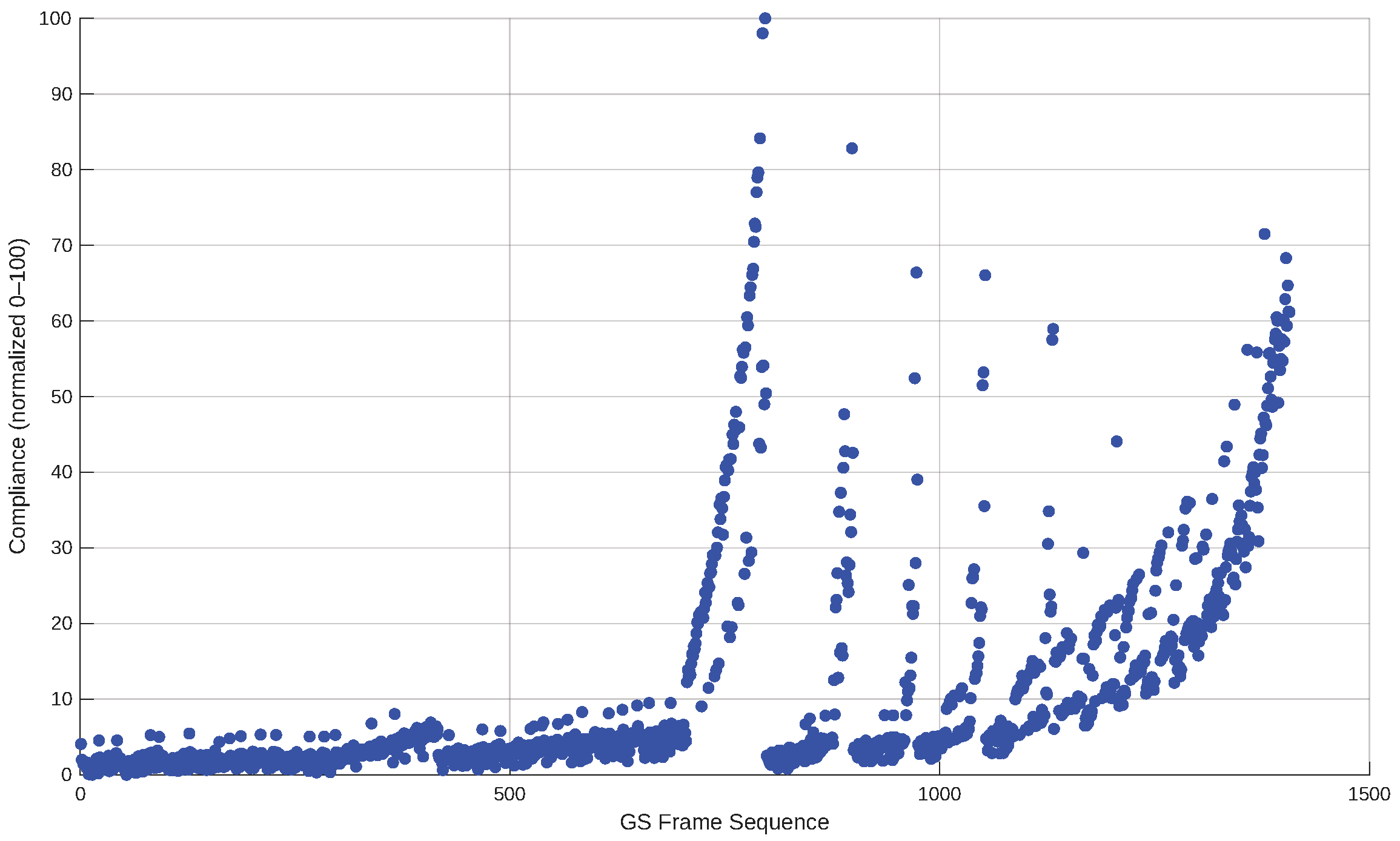
The trend in the Figure 12 plot seems to correspond to the clusters and layers of the scattered LHS plot here in Figure 11. Those frames with smaller compliance are those with relatively smaller bay width and story height. Though it is difficult to generalize, frames with a larger number of bays and stories also have smaller compliance. Larger compliances correspond to fewer bays and more stories.

80:20% data split is used to train the sparse Gaussian Process model. Out of the 20% test data, half of it is systematically split from the near optimum region, which is later used to compute the top k accuracy. And a K-fold cross-validation with K = 5 is implemented. The performance of the model returned less RMSE and MAE with values of 3.927 and 2.3031, respectively. The coefficient of determination $R^2$ 0.9963 is also quite convincing. 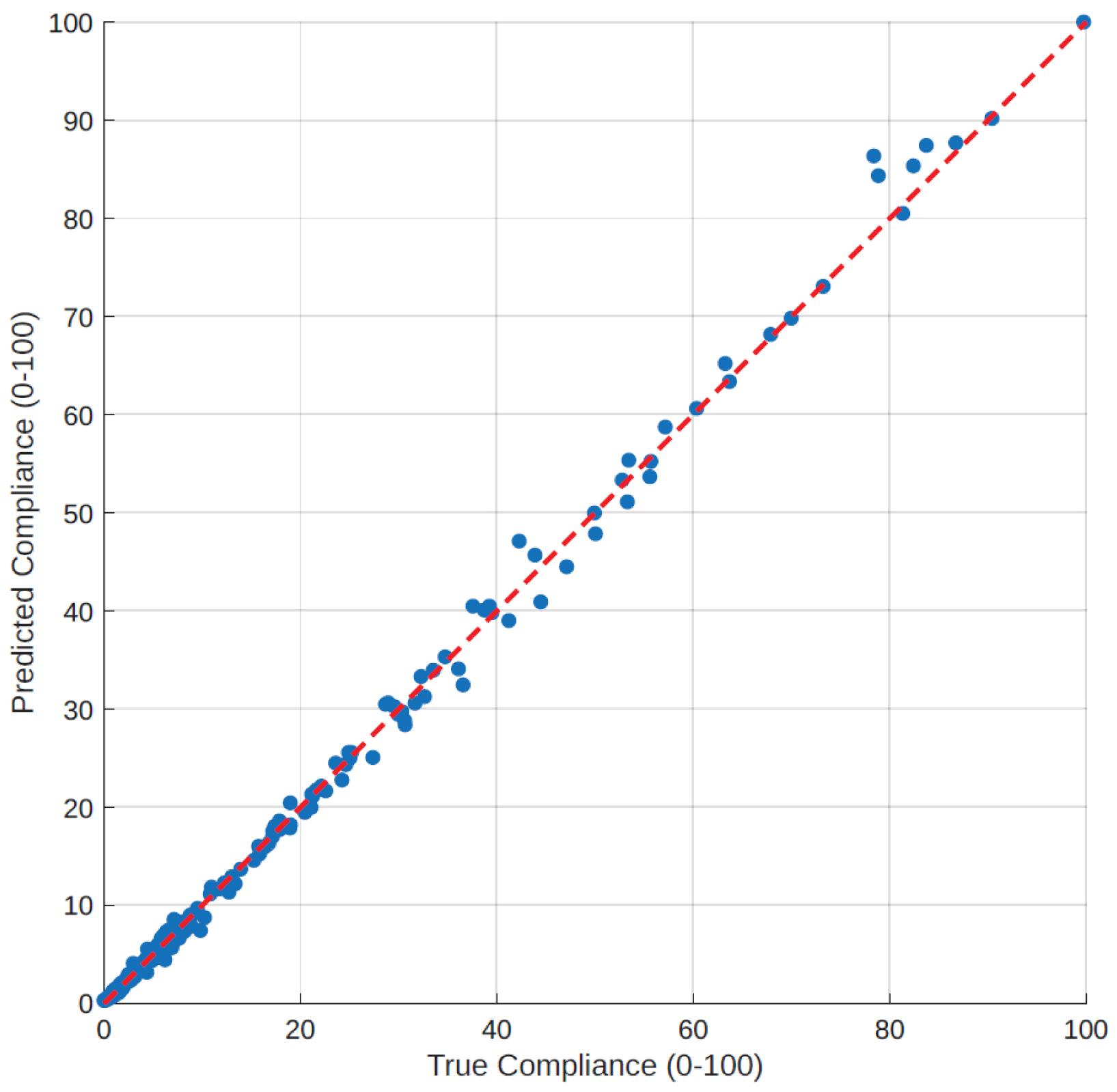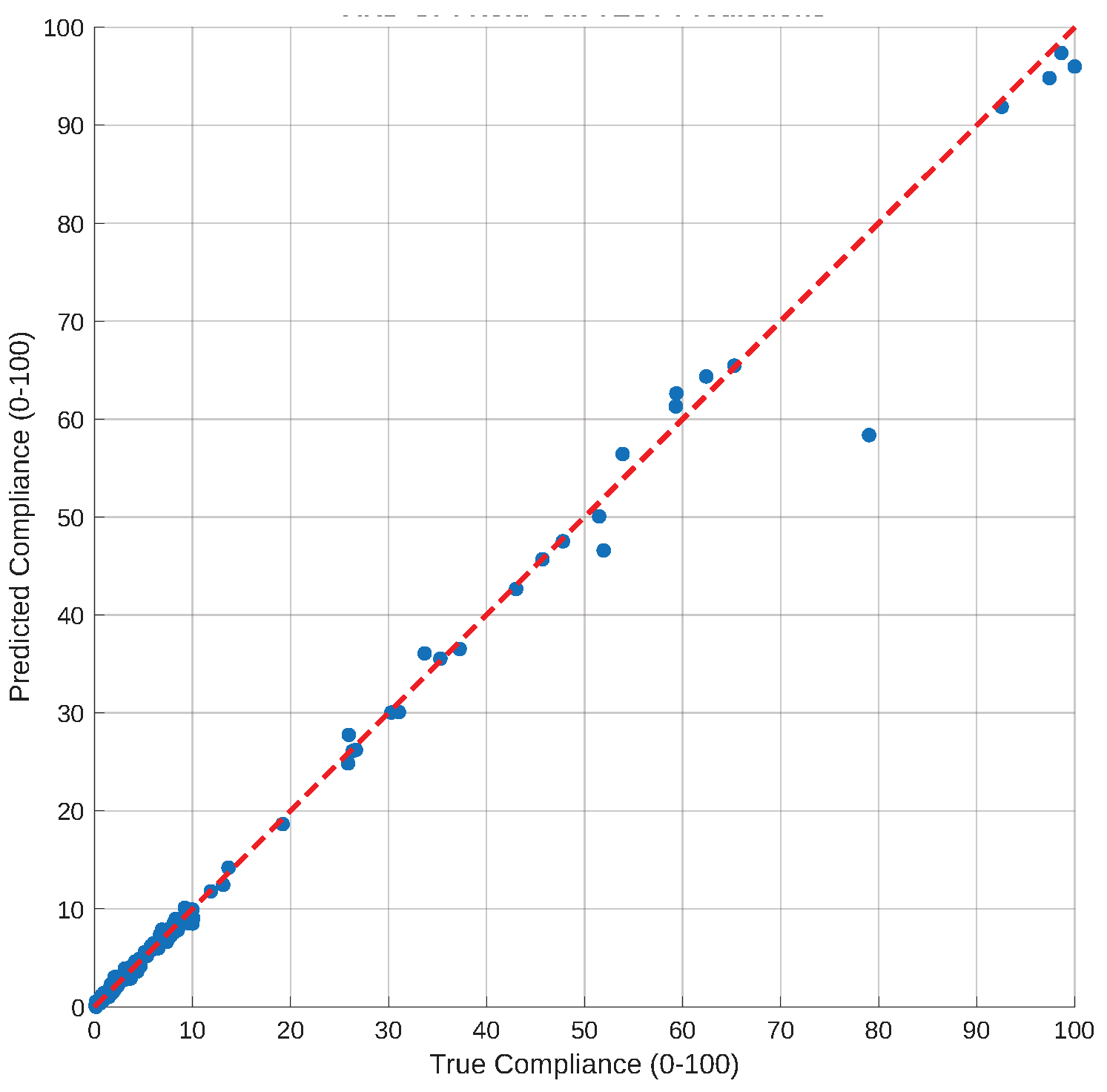Figure 13 shows the model performance on the test dataset with RMSE of 3.3519, MAE of 1.796 and $R^2$ of 0.9971.

The final step to identify potential frame/s for topology optimization out of a large domain of potential frames is making a prediction of the compliance of the remaining frames using the trained model.

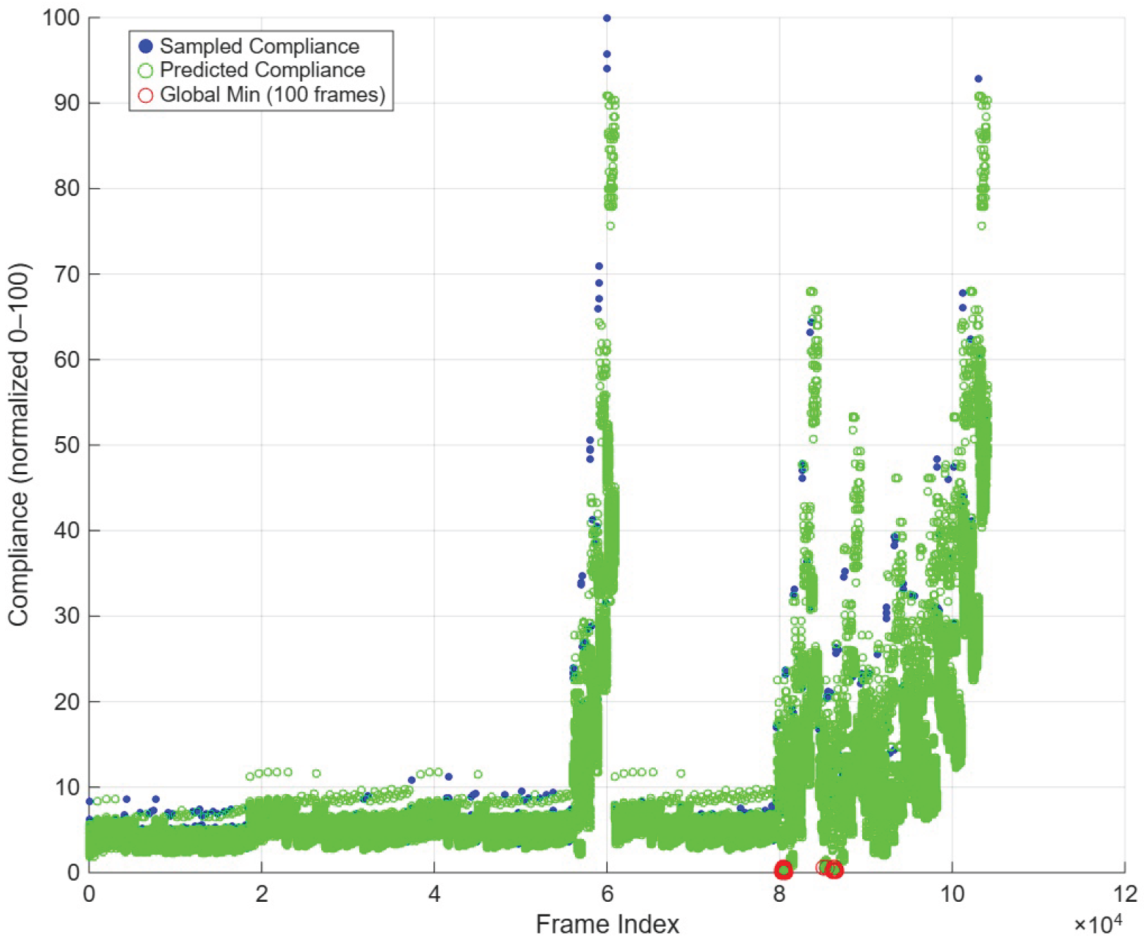
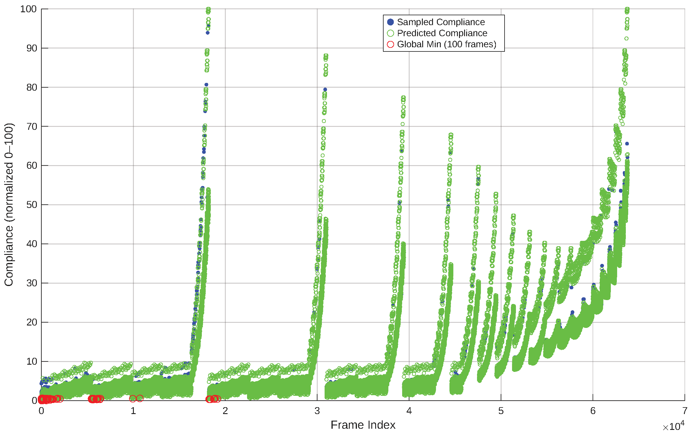
Therefore, a prediction is made for the remaining 62,377 frames. For the sake of visualization, 100 candidate frames are highlighted based on their minimal compliance score.

From Figure 14, it is observable that the prediction is fitting to the existing computed samples. All the frames within the first cluster, up to around 15,000 frames, have the maximum number of bays, the number of stories within the given domain, and the interval width. A frame with a larger number of bays and with relatively larger story height also returns smaller compliance (frames 5592 and 9944).

Frames within the same cluster are affected by their height in the story and the width of the bay. Frame 3, for example, has less compliance than Frame 111 because the latter has a relatively larger story height at its second story. Hence, those frames with the maximum number of bays and maximum number of stories, being other criteria considered here kept the same, are preferably returning the lowest compliance, hence could be chosen for compliance minimization as potential ground structures.

The advantage of this graph-based LHS and GP-guided selection over naive random candidate selection is twofold. First, graph-based LHS ensures structural diversity across the sampled frames covering variations in bay count, story count, connectivity level, and geometric perturbation rather than clustering around geometrically similar configurations as random sampling would. Second, the trained GP model ranks all remaining frames by predicted compliance, enabling targeted identification of low-compliance candidates across the full frame population without exhaustive FEM evaluation. As demonstrated in Figure 14, this combined mechanism ensures that candidates forwarded to PSO are both structurally representative and compliance-efficient, significantly reducing the computational cost of downstream topology optimization.

The ARD kernel automatically assigns different length scales to each graph-based feature. Features related to connectivity and path length (e.g., number of edges, graph diameter, average betweenness centrality) receive significantly shorter length scales than geometric spread features, indicating that they are more influential for compliance prediction.

6.3.6. PSO Optimizer Population Selection

The particle swarm is initialized using a volume-consistent warm start rather than purely random areas. For each ground structure, the total length of the meshed elements is used to determine a uniform reference area $A_0$ such that, if all elements were assigned this area, the resulting structural volume matches the target volume implied by the prescribed volume fraction. This baseline $A_0$ is then clipped to the admissible interval $[A_{\min },A_{\max }]$ and used as the center of the initialization. Around this volume-consistent baseline, Gaussian perturbations scaled by the range $A_{\max }-A_{\min }$ and controlled by a noise level are added to generate the initial particle positions, after which all areas are projected back into $[A_{\min },A_{\max }]$. In this way, all particles start from designs that are consistent with the volume constraint in an average sense, while the stochastic perturbations retain sufficient diversity; as a result, very poor (extremely stiff or nearly void) initial designs are avoided, early compliance values remain bounded, and the PSO iterations tend to be more stable and efficient.

6.3.7. Compliance Minimization of Selected Candidate Frames Using PSO Optimizer

Now, iteration-based topology optimization can be applied to any desired number of frames with smaller compliance according to Figure 14. Alternatively, if there is a strong desire to specific number of bays or stories, or bay width and story height, or their combinations, frames could be selected from an appropriate cluster or region from the candidate GS selection map shown in Figure 14.

The final step could either be computed by considering only the volume constraint to attest the appropriateness of those selected frames as candidate ground structures, or constraints that map the real-world scenario could be considered.

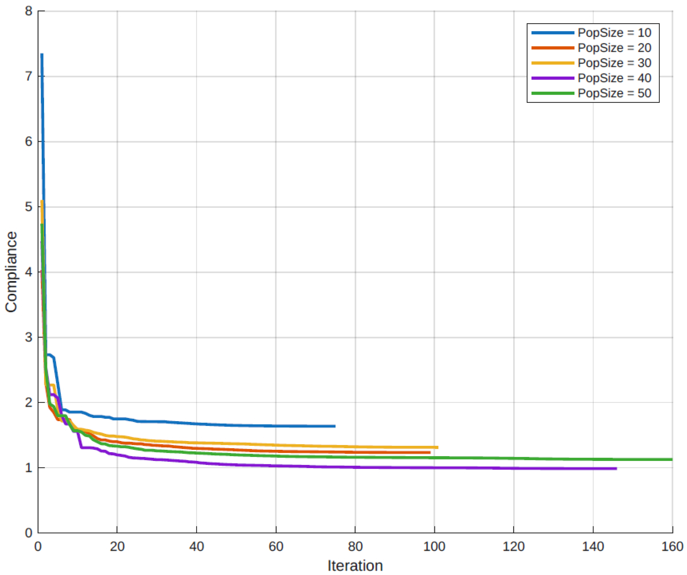
A population size of 40 was identified as optimal for the 1:1 frame aspect ratio as shown in Figure 15, and the remaining optimization was performed using this population size.

An optimization strategy based solely on the minimum compliance over all runs does not necessarily yield a structurally efficient frame with few members or a stable response after element removal. Instead, for each run, we first extract the minimum compliance attained during the PSO iterations and use it in a combined final score that accounts for (i) the best compliance reached in that run, (ii) the ratio of active to original elements, and (iii) the compliance validation $C_v$, so that sparser and structurally robust frames are preferred over denser ones with similar compliance.

For a fixed removal threshold $n_r$, this final-score metric is evaluated for all runs. The run with the minimum final score is then selected, and in a second step $C_v$ is refined for that run only, in order to further improve sparsity without compromising structural performance.

The final score used for run selection is given by

$$\mathrm{FinalScore}=C_{\min }+\alpha {\displaystyle \frac{N_{\mathrm{active}}}{N_{\mathrm{orig}}}}+C_v,$$

(36)

where:

• $C_{\min }$ is the minimum compliance over the PSO iterations for a given run,
• $N_{\mathrm{active}}$ is the number of active elements after removal,
• $N_{\mathrm{orig}}$ is the total number of original elements,
• $\alpha$ is a weighting factor controlling the influence of sparsity, taken as 1 here
• $C_v$ is the compliance validation.

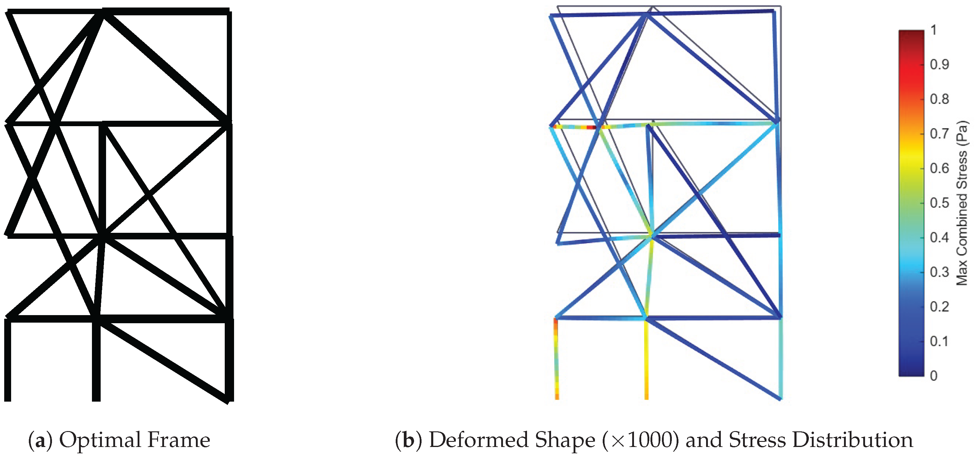
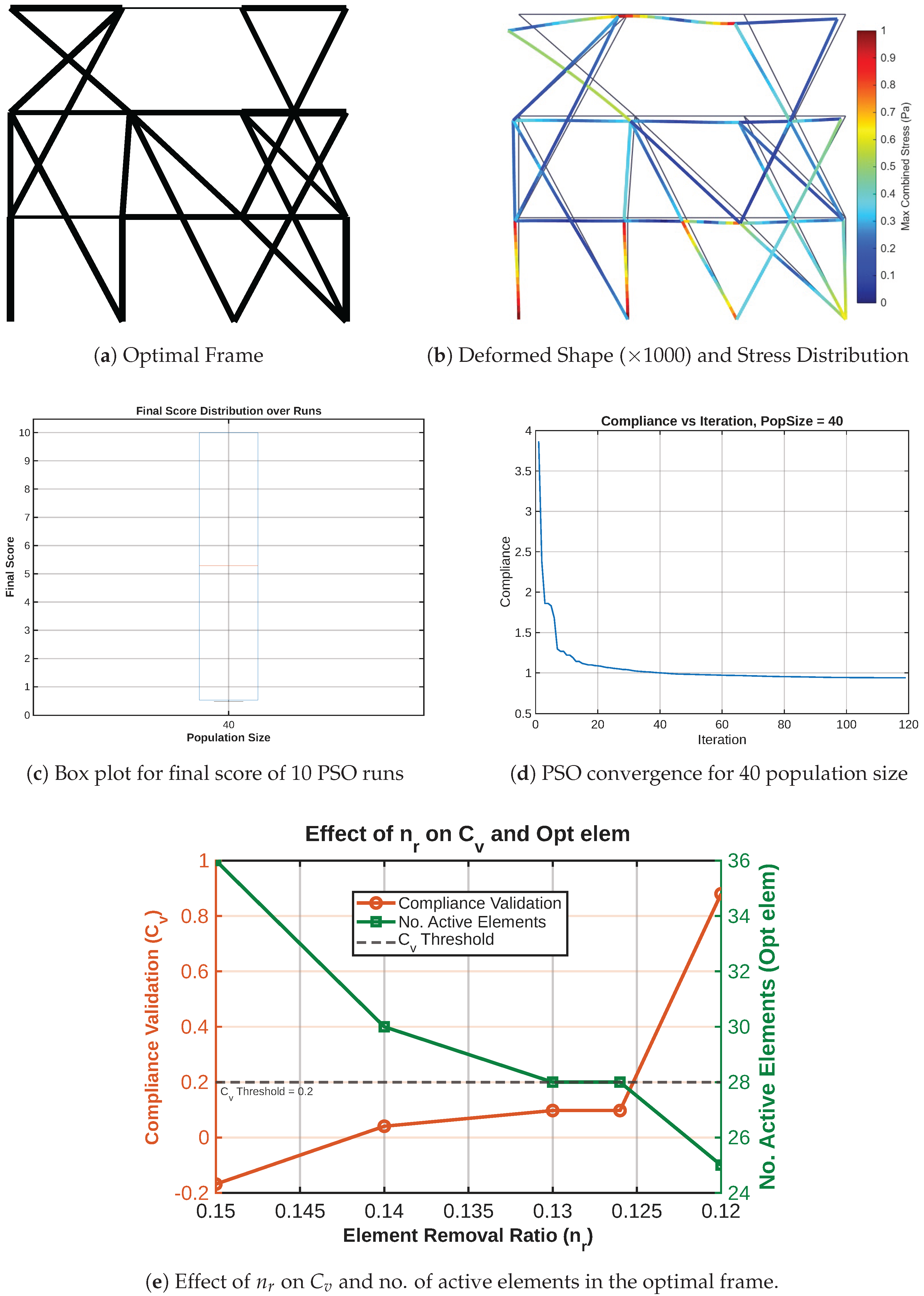
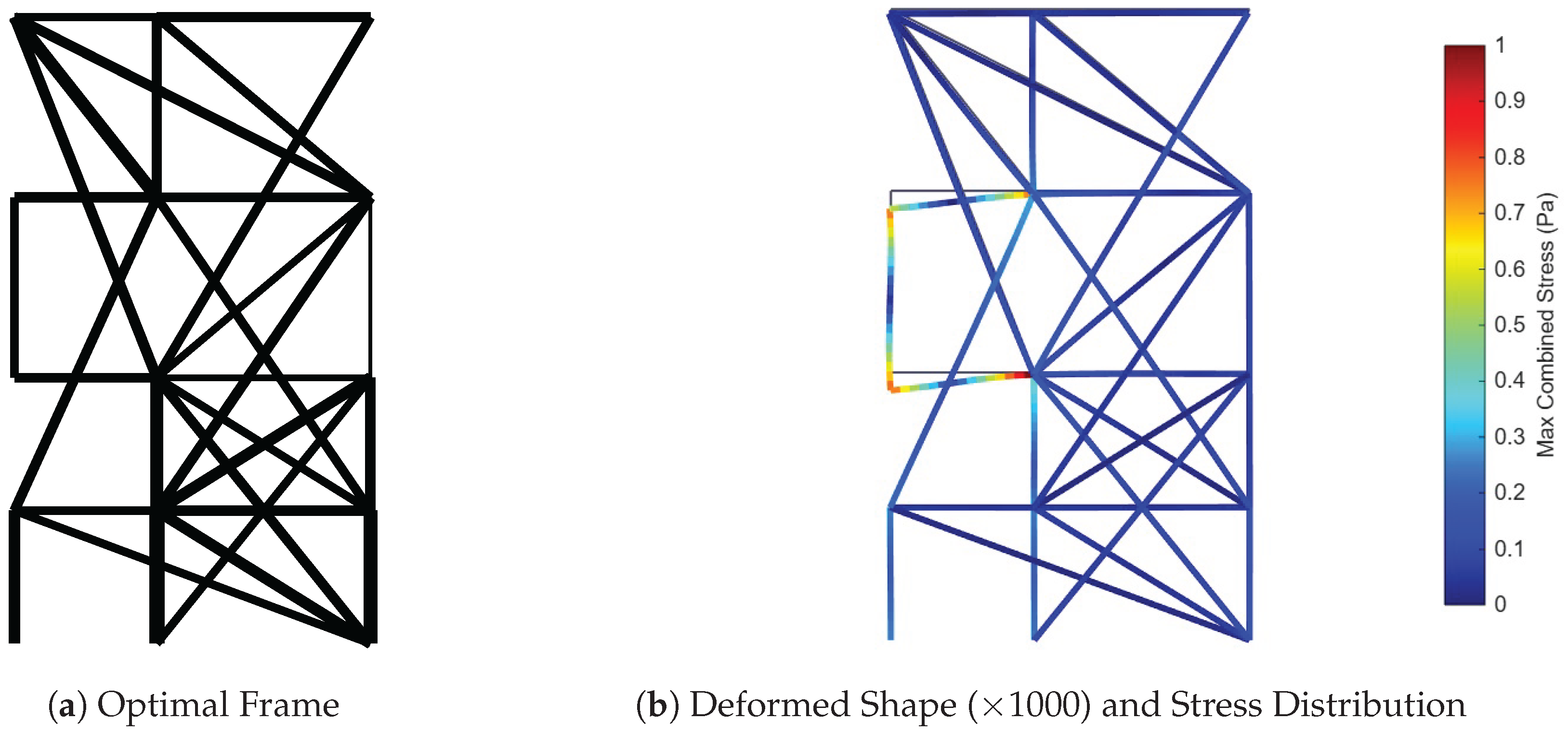
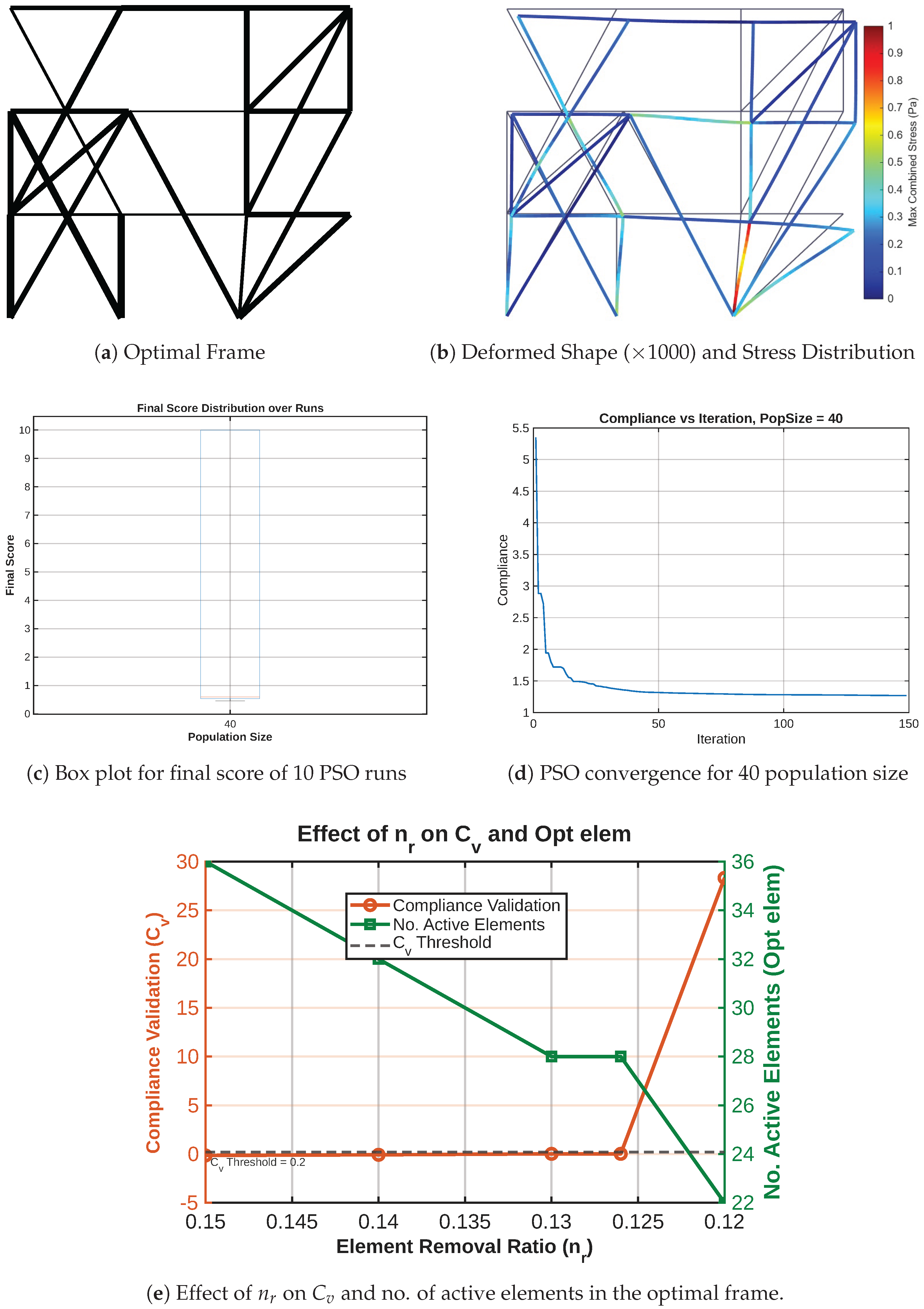
The verification procedure for frame index 24, as shown in Figure 16a, reserved only 46.1% ($1-V_f$) of the initial elements domain. The increase in compliance after element removal is limited to 9.8% only. As the frame is mainly for building purposes, thinner beams are kept from removal. The minimum area accounts for 0.38 of the normalized area scale, indicating that a considerable number of elements are retained at the minimum allowable area. This is attributed to the exclusion of floor beams from the element removal criterion, as their continuity is necessary to ensure practical slab support at every story level based on the assumption considered in this work. It is worth noting that without this floor beam retention requirement, the optimal frames would consist of significantly fewer elements, yielding sparser and more material-efficient topologies. The deflected shape in Figure 16b is scaled up by 1000 times.

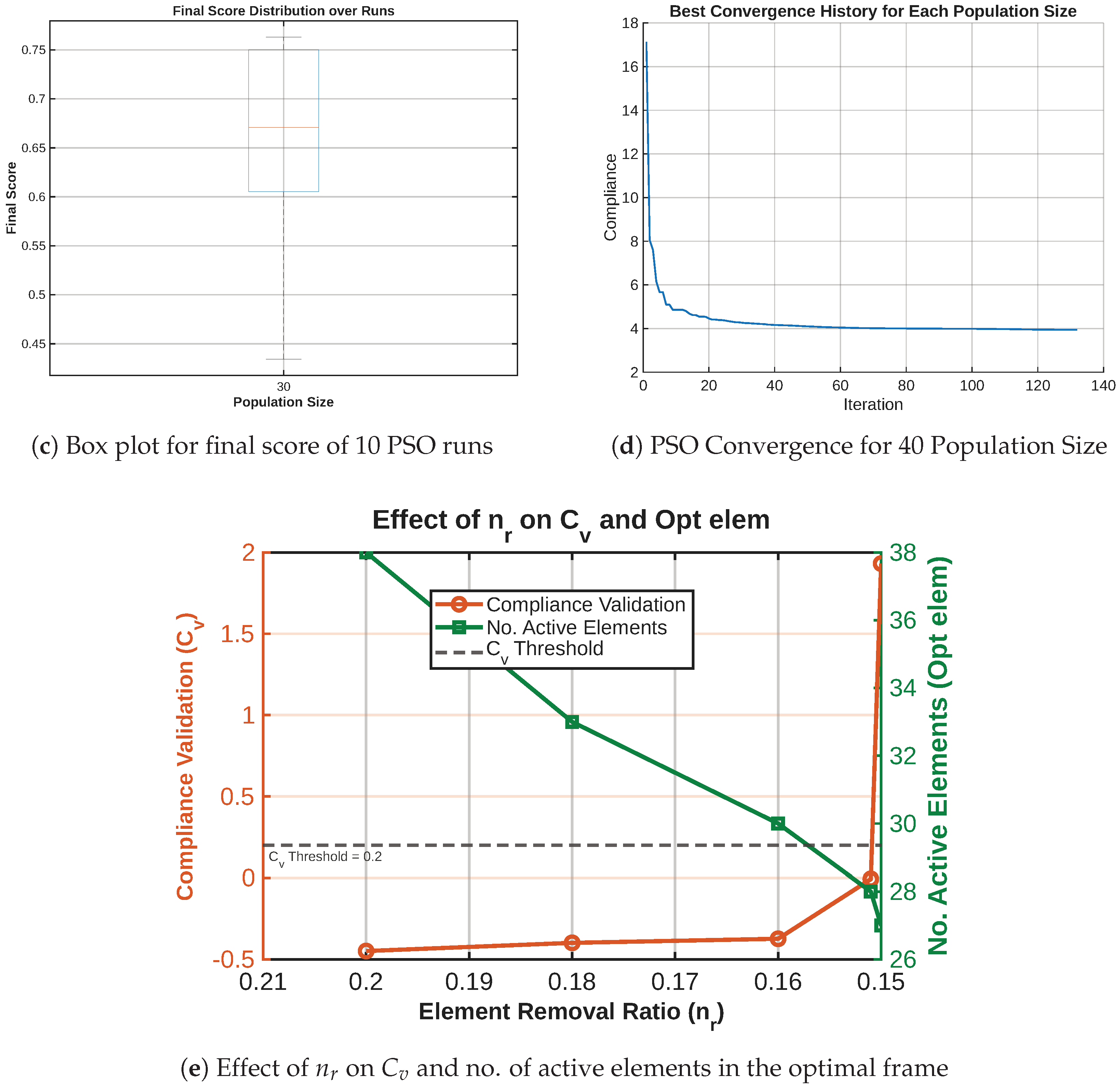
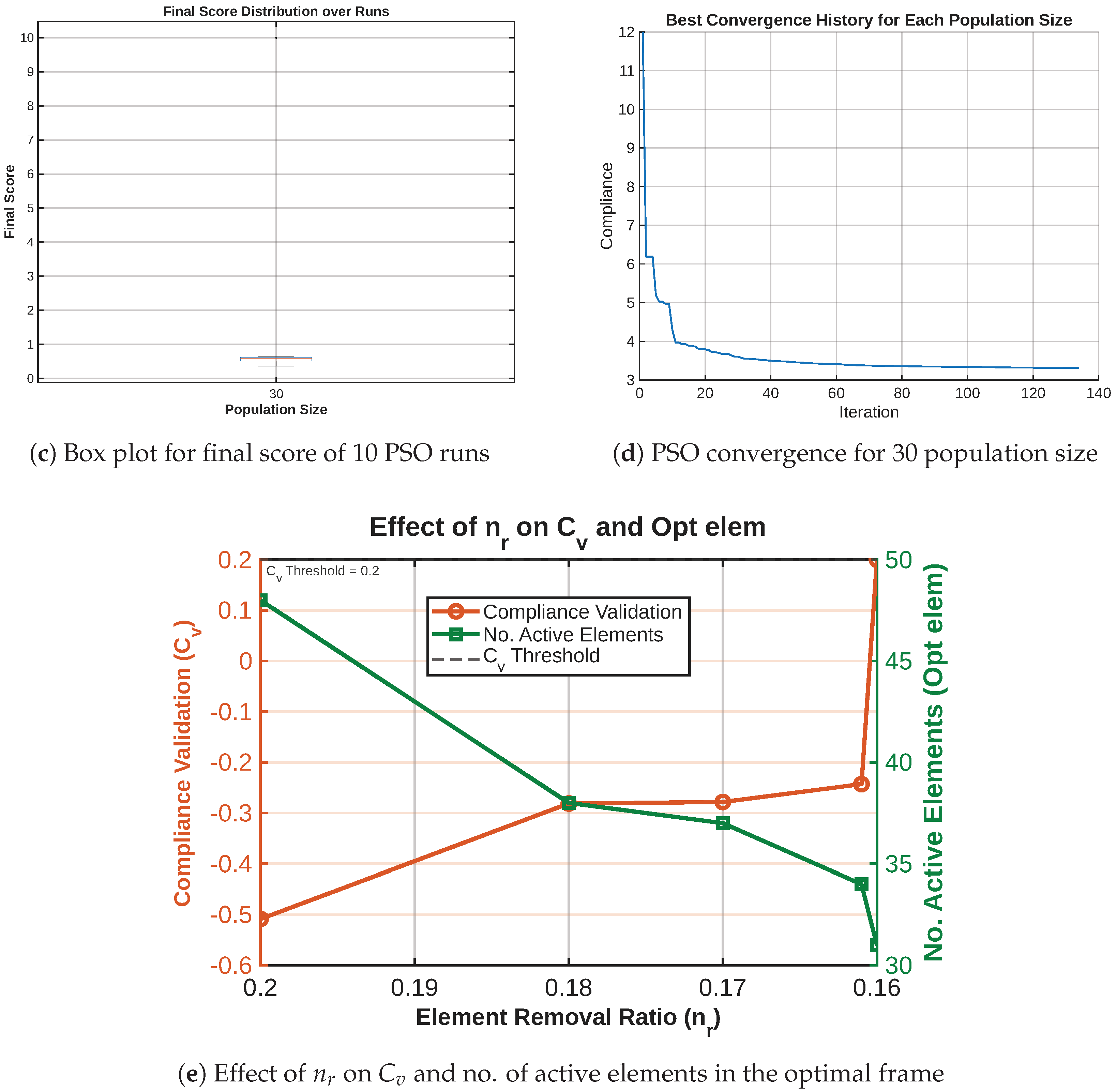
As can be observed in the convergence plot in Figure 16d, different population sizes of the PSO optimizer were implemented, and an early-stage compliance tolerance of ${10}^3$ was used with 10 iterations of patience. Accordingly, the population size of 40 returned the least compliance, and it is adapted throughout the case study. For the selected population, the PSO optimizer was run 10 times with different seeds, and the compliance is visualized using a box plot in Figure 16c. PSO runs with optimal $Cv$ greater than 0.2 are penalized with the maximum final score. Those runs in which the optimal frames after element removal do not increase their compliance more than 20% are reserved. Out of the remaining eligible runs, the one with optimal frame convergence plot is presented in Figure 16d. The optimal frame is then further updated for different element removal ratios $n_r$, and then the final optimal frame with a lesser number of elements while $C_v$ does not exceed 0.2 is considered. The smallest $n_r$ on such plots results in a sudden increase in $C_v$. This is mainly associated with large deflection on the free end of the edge beam following the removal of all supporting elements at that node.

The optimal frame Figure 17a was mainly transmitted on diagonal elements rather than on vertical columns. The pattern of their arrangement also contributed to larger space formation.

The volume fractions of 0.5–0.55 (

Table 3. Summary of Optimal Frame Parameters.

Frame Index	No. Elem	Opt Elem	${\mathit{V}}_{\mathit{f}}$	${\mathit{n}}_{\mathit{r}}$	${\mathit{C}}_{\mathit{v}}$	Norm ${\mathit{A}}_{\mathbf{min}}$
24	69	28	0.539	0.126	0.098	0.38
5464	69	28	0.503	0.126	0.020	0.36

) indicates RC frame efficiency, surpassing benchmarks in

Table 4. Volume Fraction Comparison in Topology Optimization Literature.

Structure Type	Vf Range	Vf Definition	Ground Structure	Notes
Steel trusses [41]	0.10–0.25	$V_{\mathrm{opt}}/V_{\mathrm{domain}}$	Dense/fully connected	Unrealistic for RC
Steel frames [38]	0.35–0.50	$V_{\mathrm{opt}}/V_{\mathrm{allowed}}$	Dense GS	Stress-based
RC beams [30]	0.40–0.60	$V_{\mathrm{opt}}/V_{\mathrm{concrete}}$	Truss-continuum	ASCE benchmark
RC frames [this work]	0.5–0.6	$V_{\mathrm{opt}}/(\sum A_{\mathrm{i},\max }{L}_i)$	Sparse/systematic	addressed constraints

despite constructability constraints (min. rebar/aggregate dims). In contrast, steel truss and frame studies that achieve much lower volume fractions typically employ fully connected or very dense ground structures with highly slender members and density based formulations, often without the constructability constraints that govern RC detailing [1,2,3,4,26,33,34,38]. The present Vf range therefore reflects a deliberate compromise between compliance minimization and RC feasibility, rather than a limitation of the proposed enumeration or optimization procedure.

The systematic GS generation, realistic bay widths (3–7 m), story heights (2.8–4 m), limited connectivity (Level 1/2), and nodal perturbation ($\delta =0.2$ m) yield sparse, practical topologies. Unlike dense steel truss/frame topology optimization’s single fully connected GS (enabling unrealistically low Vf via thin, non-buildable members), this balances compliance minimization under gravity loads with RC feasibility.

6.4. Methodological Context and Volume Fraction Interpretation

The use of PSO for frame topology and sizing optimization is consistent with recent applications in isogeometric topology optimization [35] and multiobjective structural design [36,37]. While PSO offers derivative-free global search suitable for the discrete, non-convex design space of RC frames, it also introduces run-to-run variability and sensitivity to parameter tuning (Section 6.1). Studies on swarm intelligence in topology optimization [21] and multiobjective RSM-NSGA-II frameworks [23] demonstrate similar trade-offs between exploration capability and convergence consistency.

The volume fractions of 0.5–0.55 reported in Table 3 and Table 5 may appear high compared to steel truss topology-optimization studies that achieve Vf = 0.10–0.25 [38,39,40,41]. However, direct comparison is misleading for three reasons:

First, RC members are physically bounded by minimum dimensions required for aggregate flow and rebar clearance, which preclude the infinitesimal member sizes often allowed in steel topology optimization. Studies on manufacturability-aware topology optimization [26,33,34] similarly report higher Vf when minimum feature size or joint-complexity constraints are enforced.

Second, the topology rule that preserves floor beams to ensure slab support (Section 4.8) introduces small compliance penalties that are secondary to detailing feasibility and structural continuity [30]. Relaxing this requirement would yield sparser configurations with Vf ≈ 0.35–0.40, but at the cost of requiring additional post-optimization slab-support verification.

Third, the present work defines Vf relative to the fully solid ground structure with maximum area Amax (Equation (12)), whereas some steel studies define Vf relative to a design domain bounding box, which can yield nominally lower values.

Within the RC optimization literature, the present Vf range is comparable to or lower than reported values for truss-continuum RC beam optimization (Vf = 0.40–0.60, [30]) and RC frame optimization using genetic algorithms (Vf ≈ 0.50–0.55, [13]), while maintaining compliance-based stiffness efficiency and realistic bay/story geometry.

6.5. Frame with 1:1.5 Aspect Ratio

Tall frames could be represented by this case. The procedure is once again the same. A total of 104,032 GS are generated from 1870 basic GS with a node location interval of 0.5, 0.5 as shown in Figure 18.

6.5.1. Effect of Sampling Ratio and Performance of Multiple Models

Apart from sparse GP and sparse GP ARD, support vector machine (SVM), random forest (RF), and gradient boost (GB) models were used and compared. In multiple cases, the sparse GP could be preferable. For the $(0.5,0.5)$ nodal interval range, the performances of these models are summarized in Figure 19.

Different graph-based LHS sampling ratio sensitivity is recorded. $1\%$ sampling least performance given the fact that the sampling is smaller. The $5\%$ sampling has the best performance. When observed in association with the near-optimal performance evaluation in terms of the metrics reported in Figure 20. The hit-rate score of $5\%$ sampling, which is $0.9$, is the highest at the top $k=10$ optimal frames. It also has the smallest median true relative gap of $0.0458$. Within the selected $5\%$ sampling, the sparse GP (ARD) showed the best performance, and accordingly, the model is preferred across all the case studies.

6.5.2. Top-k Ranking on the Validation Pool

After 10% sampling for the sake of computational burden, 1971 unique samples are returned.

A sparse Gaussian Process model is trained using the computed compliance of these samples. The 5-fold k-cross-validation resulted in $RMSE$, $MAE$ and $R^2$ values of 3.9712, 1.6228 and 0.989, respectively. The model performance on the test dataset, as shown in Figure 21, has $RMSE$, $MAE$ and $R^2$ values of 2.6704,0.789,0.9923, respectively. The hit rate and the median true relative gap are 0.8 and 0.035, respectively. A total of 102061 frames received their compliance prediction using the trained model. In addition, the desired number of frames is sampled based on their compliance value.

The prediction map for the 1:1.5 aspect ratio frame is shown in Figure 22. Optimal frames are highlighted with red color.

6.5.3. PSO Optimizer Population Selection

Minimum compliance is recorded for a population size of 30 with a value of 3.672 as shown in Figure 23. Hence, it is implemented for the optimization of both the frames considered in this case study and the aspect ratio.

It can be observed that the optimal frames still consist of more elements than would be expected in a similar structure made of steel. This could be primarily due to two factors. First, the compressive strength of RC is significantly lower than that of structural steel, especially under gravity loading as in the current case. This reduction in compressive capacity has a substantial impact on the structural response, requiring more load-bearing elements in RC designs. Second, since the frames are intended for building applications, beam elements with even smaller area are preserved from removal. This constraint leads to an increased number of elements and forces the optimizer to follow less efficient load paths.

The contribution of diagonal elements largely replaced the need for floor columns in most of the stories. As expected for an optimal load path, it is rare to see diagonal elements becoming discontinuous immediately below their lower connected nodes. Such discontinuities result in load being transferred to the beams, which are primarily designed to resist bending rather than axial loads like columns. An example of this can be seen at the second story, third bay node in Figure 24a. This discontinuity correlates with an observable increase in floor deformation in that region.

Table 5 shows the result of optimal frames with aspect ratio 1:1.5. Here as well, the volume fraction remains within the spectra of 0.5–0.55 range.

The complete removal of vertical elements except the ground floor could be seen in Figure 25a as inclined elements are favored on the left edge of the frame.

Table 5. Summary of Optimal Frame Parameters.

Frame Index	No. Elem	Opt Elem	${\mathit{V}}_{\mathit{f}}$	${\mathit{n}}_{\mathit{r}}$	${\mathit{C}}_{\mathit{v}}$	Norm ${\mathit{A}}_{\mathbf{min}}$
56,193	79	31	0.53	0.16	0.20	0.411
56,200	79	28	0.539	0.151	−0.007	0.423

Table 5. Summary of Optimal Frame Parameters.

Frame Index	No. Elem	Opt Elem	${\mathit{V}}_{\mathit{f}}$	${\mathit{n}}_{\mathit{r}}$	${\mathit{C}}_{\mathit{v}}$	Norm ${\mathit{A}}_{\mathbf{min}}$
56,193	79	31	0.53	0.16	0.20	0.411
56,200	79	28	0.539	0.151	−0.007	0.423

7. Conclusions

This work contributes a novel framework for the topology optimization of reinforced-concrete building frames, addressing the unique structural characteristics of RC systems, such as sparse connectivity and rigid orthogonal joints. By developing a graph-based ground-structure generation method combined with Latin hypercube sampling and surrogate modeling, the proposed approach enables efficient exploration of a vast configuration space without relying on full-scale iterative optimization for every candidate.

The use of a sparse Gaussian Process model to predict compliance values across unsampled frame configurations proved effective in identifying structurally promising ground structures. These were subsequently refined through compliance minimization using particle swarm optimization, yielding optimal frame designs for two representative domains with distinct aspect ratios.

The case study demonstrated that the optimal load transfer path for frames subjected to gravity loads at the top nodes involved an integrated system of vertical and diagonal elements, which led to the removal of vertical elements such as columns on the intermediate and lower floors.

Importantly, the integration of story beams, exempt from the element removal rule, allowed for the retention of essential structural integrity while achieving volume fractions below 0.55 in all optimized cases. A notable proportion of elements converge to the lower area bound, a direct consequence of enforcing floor beam continuity for slab support. Relaxing this requirement would naturally lead to considerably sparser structural configurations with a reduced element count. This demonstrates that the proposed approach holds significant potential for generating efficient RC frame designs. The presented methodology offers a scalable and data-informed path forward for early-stage structural exploration and optimization in RC building design.

The candidate GS selection map, which illustrates considered frames alongside their predicted compliance at an early stage, not only avoids nonstrategic or non-systemic use of GS but also streamlines the selection process. This significantly reduces the computational cost and time required for downstream tasks. Moreover, the map serves as a key reference for understanding the influence of frame parameters and enables candidate GS selection based on specific sub-parameters, such as the desired number of bays and stories required for the structure.

From a structural design perspective, the present formulation should be interpreted as an early-stage, service-level screening tool that identifies promising RC frame topologies under linear-elastic stiffness criteria and practical connectivity constraints, rather than as a complete design procedure. Detailed verification of ultimate limit states, crack control, member instability, and reinforcement detailing must follow using established nonlinear finite-element and code-based approaches such as those reported for RC beams, frames, and composite members [13,14,15,30,31] and prescribed in [27].

This study has several limitations. The analysis is restricted to two-dimensional RC frame models and assumes linear-elastic material behavior, which does not capture nonlinear cracking or yielding effects. Gravity loads and idealized notional lateral loads are considered, while other load combinations (wind, seismic with appropriate factors, multi-directional effects) and time-dependent effects (creep, shrinkage) are not explicitly treated.

In its current form, the framework already incorporates several RC-specific features, including transformed-section stiffness modeling, elastic stress limits, a topology rule that preserves floor beams while selectively removing columns, and a post-optimization compliance-validation step. Nonetheless, detailed shear design, ductility and capacity-design checks, explicit drift limits, and nonlinear RC behavior remain outside the present scope and constitute natural extensions.

Future extensions should integrate these filters either as hard constraints in the ground-structure enumeration or as penalty terms in the compliance objective. In this sense, the proposed pipeline is complementary to existing RC optimization frameworks based on genetic algorithms [13], machine-learning-driven progressive collapse checks [15], and continuum-based RC topology optimization [30], providing a systematic way to narrow down candidate layouts before more computationally intensive inelastic simulations and design checks are carried out.