Bending Performance of Steel–Concrete Composite I-Beam with Corrugated Steel Web Under Thermo-Mechanical Coupling

Abstract

An analytical model is developed to investigate the bending performance of composite I-beams with corrugated steel web (CSW) under thermo-mechanical coupling. The CSW is idealized as an equivalent orthotropic plate according to the principle of stiffness equivalence and heat conservation. The steady-state temperature field of the composite I-beam cross-section is obtained using the finite difference method. Based on thermoelastic theory, analytical solutions for the stresses and displacements of the composite beam subjected to thermo-mechanical loads are derived by the eigenvalue method and transfer matrix method. The results obtained in this study are compared with available experimental results from a steel–concrete composite bridge deck, ABAQUS (version: 2023) finite element simulations, and the temperature distributions specified by JTG D60-2015, AASHTO 2017 and DIN 101. In addition, the superposition principle for thermo-mechanical conditions is verified by the analytical forms of stress and displacement solutions. And the research results show that increasing interfacial stiffness restrains the relative thermal deformation between the concrete slab and the steel I-beam, thereby increasing temperature-induced stresses and deformations. Finally, a partial thermal insulation method is proposed to mitigate temperature gradients, thermal stresses and upward thermal deformation, thereby improving the service performance of the composite beam under thermal actions.

1. Introduction

Owing to their distinct advantages in structural performance, construction efficiency and economy, steel–concrete composite I-beams with corrugated steel web (CSW) have been widely used in bridge engineering in recent years [1,2,3]. This type of composite beam generally consists of a concrete slab, upper and lower steel flanges, and a CSW connected by shear connectors. The adoption of CSW not only reduces the structural self-weight but also enhances web stability, making this type of structure attractive for engineering applications. Due to the corrugated geometry of the web, the CSW possesses high transverse stiffness and stability but relatively weak longitudinal stiffness, exhibiting mechanical properties that deviate from those of conventional isotropic materials. In practical service conditions, in addition to conventional loads, environmental temperature variation also plays an important role in the structural response [4]. Moreover, the different thermal properties of concrete and steel may lead to a non-uniform temperature field along the beam depth and near the steel–concrete interface, while the corrugated web further affects the heat-transfer path. These features indicate that the bending behavior of composite I-beams with CSWs under thermo-mechanical coupling effects deserves further investigation.

Existing studies on composite I-beams with CSWs have primarily focused on their mechanical behavior under purely mechanical loads [5,6,7,8]. Through bending tests on composite I-beams with flat steel web and CSW, Zha et al. [9] investigated the influence of different web configurations on the bending behavior of composite I-beams. Abbas et al. [10] used the virtual load method to analyze flange lateral bending in composite I-beams with CSW and validated the theoretical results through full-scale four-point bending tests. These studies have considerably improved the understanding of the structural behavior of CSW composite I-beams and provided an important basis for their analysis and design. Compared with the relatively mature studies on ambient-condition mechanics, thermal actions on such structures remain much less systematically understood.

In addition to mechanical loading, environmental temperature variations are another important factor affecting the service performance of composite beams. Based on field observations, Ma et al. [11] identified two typical temperature distribution patterns under solar radiation and nighttime conditions. Through long-term temperature monitoring, Huang et al. [12] investigated the temporal and spatial temperature distribution characteristics of composite box girders with CSW and established a refined numerical simulation method validated by measured data. By means of scaled experiments, Wang et al. [13] studied the temperature distribution and thermal effects in steel–concrete composite bridge decks, and found that the temperature varied nonlinearly along the beam depth. Through indoor radiation experiments, Fan et al. [14] studied the temperature field of steel–concrete composite beam bridges and further established a refined numerical model for the solar-induced temperature field. Based on measured temperature data from a steel–concrete composite box girder bridge, Li et al. [15] analyzed the temperature field and gradient effect of the structure and further evaluated their influence on stress and deformation responses. These studies show that non-uniform temperature fields and nonlinear temperature gradients are common in composite structures. Recently, intelligent algorithms have also been introduced into the temperature-field analysis of bridges with CSWs. Zhang et al. [16] proposed a BP-neural-network-based method for predicting the temperature field of PC beam bridges with CSWs using measured data, which improved the efficiency of temperature-field prediction. Another recent study [17] established a temperature-gradient model for PC beams with CSWs in China using a random forest algorithm and long-term meteorological monitoring data. These studies indicate that machine-learning methods provide effective tools for rapid temperature-field prediction when sufficient monitoring data are available. However, data-driven approaches are usually dependent on measured datasets, whereas a mechanics-based analytical model is still needed to reveal the thermo-mechanical response mechanism and support parametric analysis.

Alongside experimental investigations, theoretical methods have also been widely employed to analyze the temperature field and thermal effects of composite beams. To investigate the thermal stresses of steel–concrete composite box girders, Shan et al. [18] established a theoretical model based on the static equilibrium of beam elements and deformation compatibility conditions. Fan et al. [19] developed a vertically discretized dimension-reduced model for steel–concrete composite bridges and achieved rapid calculation of the temperature field by combining it with a state-equation solution method. By combining finite element and theoretical methods, Xiang et al. [20] investigated the stress and shear-force distributions in a three-span continuous composite beam bridge under thermal actions. Through theoretical and finite element methods, Cai et al. [21] studied the temperature effects of composite girders with CSW considering the local longitudinal stiffness of the webs and revealed that the interfacial shear force and interface slip are non-uniformly distributed along the beam length under thermal actions. For the static design of steel–concrete composite girders, Wang et al. [22] proposed thermal load models and investigated their applicability in evaluating thermal stresses. By considering both flat and corrugated steel webs under temperature gradients, Peng et al. [23] clarified the distributions of temperature-induced stresses and interface shear forces in composite girders and highlighted the distinct thermal stress characteristics of girders with CSW. These studies have advanced the analysis of thermal effects in composite structures. Recent data-driven and surrogate modeling methods have also been increasingly used for structural performance assessment in bridge engineering. Representative studies have applied random-forest surrogate models, multi-source data-driven frameworks, multi-scale mechanical models and Bayesian-optimized deep-learning models to fatigue assessment and life prediction of bridge components [24,25,26,27]. These studies further demonstrate the potential of data-driven methods for efficient structural response prediction and performance assessment.

Although numerous analytical models have been proposed for composite beams with CSWs, the anisotropic characteristics of CSWs have received limited attention. Furthermore, most existing models for composite I-beams with CSWs are based on simplified assumptions regarding transverse shear deformation, which may result in substantial inaccuracies because of the significant shear deformation inherent to these structures. In addition, studies on the thermo-mechanical coupling effect in the bending behavior of composite beams with CSWs remain scarce.

This study aims to establish an analytical framework for investigating the temperature field and thermo-mechanical bending behavior of composite I-beams with CSWs. To account for the anisotropic characteristics of CSWs, the corrugated web is idealized as an equivalent orthotropic plate based on the principle of stiffness equivalence and heat conservation. A two-dimensional steady-state temperature-field model is developed for the cross-section, and the corresponding temperature distribution is obtained using the finite difference method. Subsequently, within the framework of thermoelastic theory, analytical solutions for the stresses and displacements of the composite beam subjected to thermo-mechanical loads are formulated using the eigenvalue method and the transfer matrix method. The thermoelastic theory does not introduce any simplified transverse shear deformation assumptions, while the thermo-mechanical coupling effect is inherently incorporated in the governing equations. The present solution is verified by comparison with existing solutions. Furthermore, the applicability of the superposition principle is examined, and the effects of interfacial shear stiffness and side insulation on the structural response are systematically investigated.

2. Theoretical Model

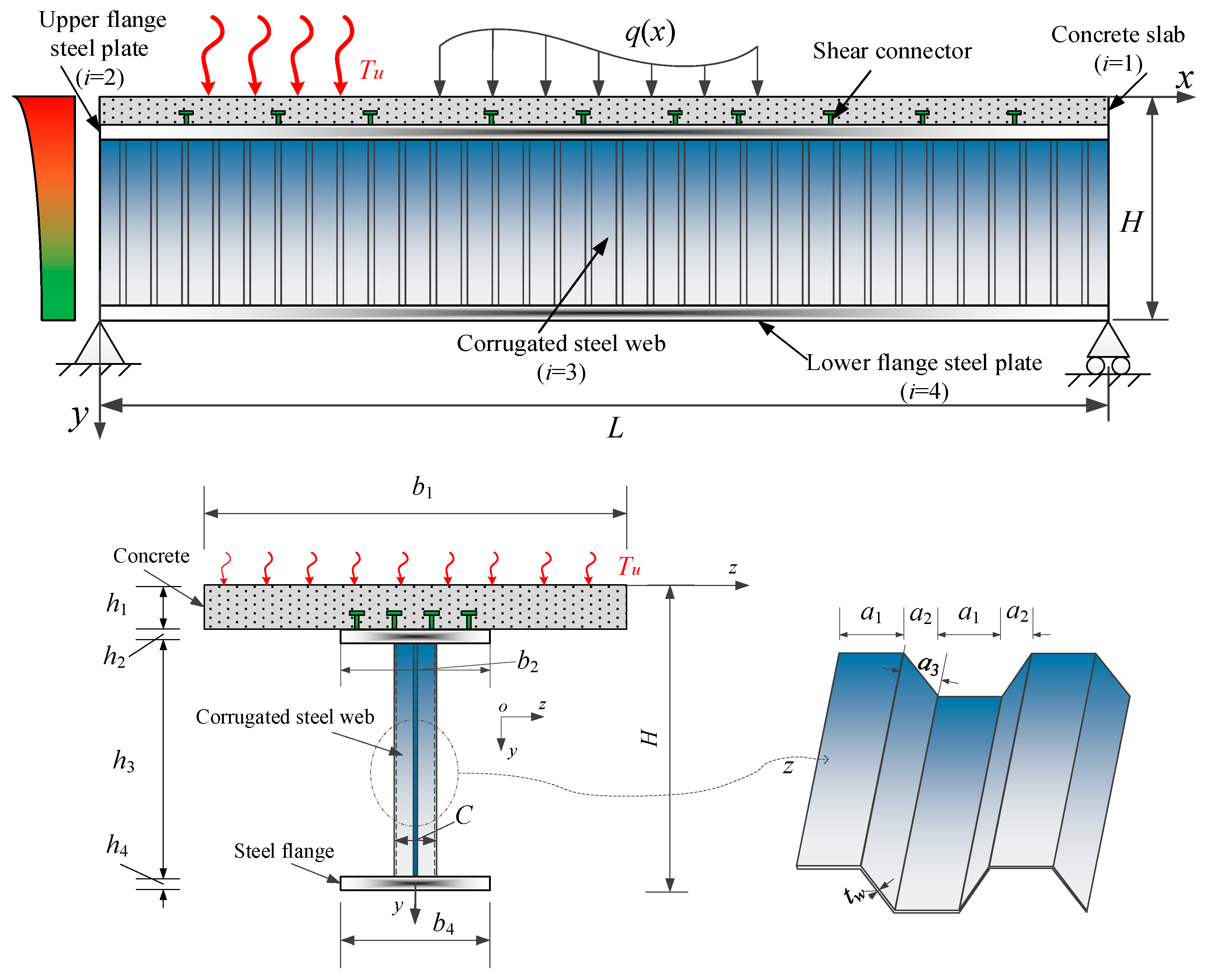
As shown in Figure 1, the object of study is a simply-supported composite beam with CSW, with length L = 45 m and height H = 2150 mm. The beam consists of a concrete slab, a CSW, and two steel flanges, where the slab-to-upper-flange interface is joined by shear connectors with an average stiffness k_s. The height and width of each layer are denoted by hi and b_i (i = 1, 2, 4), respectively, except the width of CSW is C. Within one corrugation period, the CSW thickness, corrugation angle, horizontal length, inclined length, and inclined projection are denoted by t_w, θ, a₁, a₃, and a₂, respectively. The elastic modulus, shear modulus, and Poisson’s ratio of concrete and steel are denoted by E_c, G_c, ν_c and E_s, G_s, ν_s, respectively, while the corresponding coefficients of thermal expansion are denoted by α_c and α_s.

The composite beam is subjected to external load q(x) and temperature T_u at the top surface, with heat exchange to ambient air at temperature T_a elsewhere. Since the thermal boundary conditions are invariant along the x-direction, the temperature field needs to be analyzed only on a cross-section, namely in the y-o-z plane, whereas the bending analysis can be simplified as a two-dimensional problem in the x-o-y plane.

2.1. Equivalent Coefficients

Owing to its corrugated geometry, the steel web exhibits pronounced anisotropy in the longitudinal and transverse directions. Based on the principle of stiffness equivalence, the CSW is idealized as an assimilated orthotropic plate (AOP). In the equivalent model, the AOP replaces the original CSW. Its longitudinal length and height are taken as L and h₃, respectively. The corrugated width of the original CSW is denoted by C, while the width of the AOP is defined as b₃ and is taken as the web thickness t_w, namely b₃ = t_w. The corrugated geometry is reflected by the equivalent mechanical and thermal coefficients. Accordingly, the equivalent elastic moduli E_x and E_y, the equivalent shear modulus G_xy, and the equivalent Poisson’s ratios ν_xy and ν_yx are determined based on the stiffness equivalence principle, as given in Ref. [28].

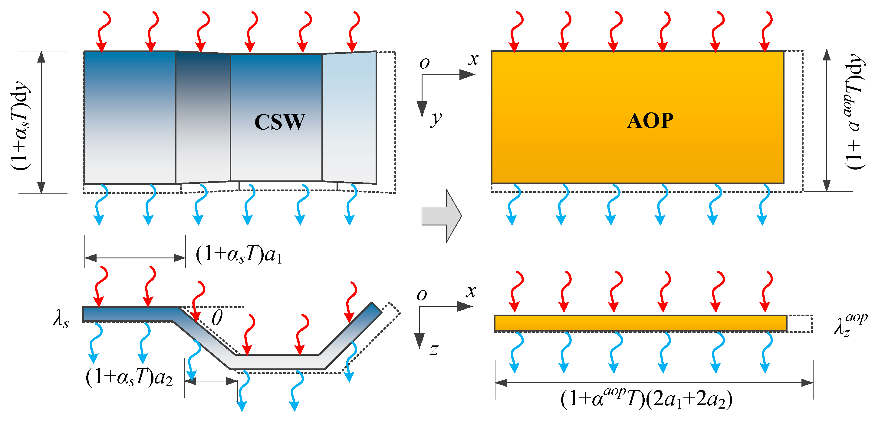
According to the principle of heat conservation, the relationship between the thermal conductivity of the AOP and that of the CSW is established, as shown in Figure 2. It should be noted that this equivalence is established under steady-state conduction. Therefore, transient heat storage is not included, and localized heat accumulation in the inclined corrugation segments is not explicitly considered. The actual CSW is idealized as an AOP by requiring that the net heat flux through one corrugation period be equal to that through the corresponding AOP under the same macroscopic temperature gradient. This assumption is reasonable when the corrugation wavelength is much smaller than the characteristic length of the cross-sectional temperature variation and when the structural response is governed mainly by a quasi-steady temperature field. Accordingly, the heat-conservation relationship can be written as

$$T{\lambda }_{s}2(a_1+{\displaystyle \frac{a_2}{\cos \theta }})t_w/dy=T{\lambda }_y^{AOP}2(a_1+a_2)t_w/dy,$$

$${\displaystyle \frac{T{\lambda }_{s}2(a_1+a_2)dy}{2(a_1+\frac{a_2}{\cos \theta })t_w/2(a_1+a_2)}}={\displaystyle \frac{T{\lambda }_z^{AOP}2(a_1+a_2)dy}{t_w}},$$

(1)

where λ_s is the thermal conductivity of steel, ${\lambda }_y^{AOP}$ and ${\lambda }_z^{AOP}$ are the equivalent thermal conductivities of the AOP in the y- and z-directions, respectively. θ, a₁ and a₂ are the geometric parameters of the CSW, t_w is the thickness of the CSW and T denotes the temperature field. Therefore, the equivalent thermal conductivities of the AOP are obtained as

$${\lambda }_y^{AOP}={\displaystyle \frac{a_1+\frac{a_2}{\cos \theta }}{a_1+a_2}}{\lambda }_s, {\lambda }_z^{AOP}={\displaystyle \frac{a_1+a_2}{a_1+\frac{a_2}{\cos \theta }}}{\lambda }_s.$$

(2)

By examining the deformation, it can be found that the coefficients of thermal expansion of the AOP in the x- and y-directions are identical to that of steel, and the relationship is expressed as follows:

$${\alpha }_x^{AOP}={\alpha }_y^{AOP}={\alpha }_s,$$

(3)

where ${\alpha }_x^{AOP}$ and ${\alpha }_y^{AOP}$ are the thermal expansion coefficients of the AOP in the x- and y-directions, respectively.

2.2. Finite Difference Solution for Steady-State Temperature

In the beam cross-section, according to heat transfer theory, the governing equation for two-dimensional steady-state heat conduction is written as

$${\lambda }_y{\displaystyle \frac{{\partial }^{2}T}{\partial y^2}}+{\lambda }_z{\displaystyle \frac{{\partial }^{2}T}{\partial z^2}}=0,$$

(4)

where T denotes the temperature field, λ_y and λ_z denote the thermal conductivities in the y- and z-directions, respectively. The concrete slab and steel flanges are treated as isotropic regions, for which λ_y = λ_z, whereas the CSW is modeled as an equivalent orthotropic region, for which λ_y and λ_z may differ. In practical bridge engineering, solar radiation, ambient temperature and wind speed vary with time, and the actual temperature field is generally transient. In this study, a steady-state temperature-field model is adopted to clarify the fundamental thermo-mechanical coupling mechanism and to evaluate the structural response under representative temperature gradients. This treatment is reasonable for slowly varying thermal actions or long-duration heating conditions, where the cross-sectional temperature field can be approximately regarded as quasi-steady. However, the present model may not capture peak thermal stresses induced by rapid environmental fluctuations. The conductive heat flux densities along the positive coordinate directions are given by Fourier’s law as

$$q_y=-{\lambda }_y{\displaystyle \frac{\partial T}{\partial y}}, q_z=-{\lambda }_z{\displaystyle \frac{\partial T}{\partial z}}.$$

(5)

In the following derivation, the face heat flux is taken as positive when entering the control cell, and the minus sign in Equation (5) is absorbed accordingly. The thermal boundary conditions are expressed by

$$\left\{\begin{array}{c}T=T_u,on the top surface\\ -n_y{\lambda }_y{\displaystyle \frac{\partial T}{\partial y}}-n_z{\lambda }_z{\displaystyle \frac{\partial T}{\partial z}}=\beta (T-T_a),on the remaining exposed surfaces\end{array}\right.,$$

(6)

where n_y and n_z are the components of the outward unit normal vector in the y- and z-directions, respectively, and β is the convective heat transfer coefficient.

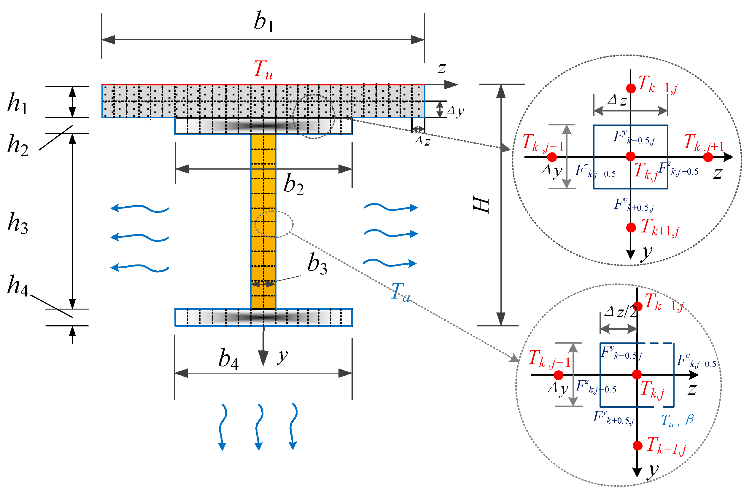
Based on the finite difference method [29], the beam cross-section is discretized into a structured grid with grid spacings Δy and Δz in the y- and z-directions, respectively, as shown in Figure 3. For an internal node T_k,j, under steady-state conditions, the algebraic sum of the heat fluxes through the four faces of the control cell is equal to zero, namely,

$$F_{k-0.5,j}^y\Delta z+F_{k+0.5,j}^y\Delta z+F_{k,j-0.5}^z\Delta y+F_{k,j+0.5}^z\Delta y=0.$$

(7)

where $F_{k\pm 0.5,j}^y$ and $F_{k,j\pm 0.5}^z$ denote the conductive heat-flux densities entering the control cell through the faces normal to the y- and z-directions, respectively. According to Equation (5), the conductive heat fluxes through the four faces are approximated as

$$F_{k-0.5,j}^y={\lambda }_{k-0.5,j}^y{\displaystyle \frac{T_{k-1,j}-T_{k,j}}{\Delta y}}, F_{k+0.5,j}^y={\lambda }_{k+0.5,j}^y{\displaystyle \frac{T_{k+1,j}-T_{k,j}}{\Delta y}},$$

$$F_{k,j-0.5}^z={\lambda }_{k,j-0.5}^z{\displaystyle \frac{T_{k,j-1}-T_{k,j}}{\Delta z}}, F_{k,j+0.5}^z={\lambda }_{k,j+0.5}^z{\displaystyle \frac{T_{k,j+1}-T_{k,j}}{\Delta z}}.$$

(8)

Substituting Equation (8) into Equation (7) yields the finite-difference equation for an internal node,

$${\displaystyle \frac{{\lambda }_{k+0.5,j}^y(T_{k+1,j}-T_{k,j})+{\lambda }_{k-0.5,j}^y(T_{k-1,j}-T_{k,j})}{\Delta y^2}}+{\displaystyle \frac{{\lambda }_{k,j+0.5}^z(T_{k,j+1}-T_{k,j})+{\lambda }_{k,j-0.5}^z(T_{k,j-1}-T_{k,j})}{\Delta z^2}}=0,$$

(9)

where ${\lambda }_{k+0.5,j}^y$, ${\lambda }_{k-0.5,j}^y$, ${\lambda }_{k,j+0.5}^z$ and ${\lambda }_{k,j-0.5}^z$ are the equivalent thermal conductivities at the interfaces between adjacent nodes. To ensure continuity of temperature and normal heat flux across material interfaces, the equivalent thermal conductivities at the half-grid faces are evaluated using the harmonic mean

$${\lambda }_{k+0.5,j}^y={\displaystyle \frac{2{\lambda }_{k,j}^y{\lambda }_{k+1,j}^y}{{\lambda }_{k,j}^y+{\lambda }_{k+1,j}^y}},$$

and the remaining interface conductivities are obtained analogously.

For the nodes located on the top surface, the temperature is directly determined by the prescribed boundary condition, i.e., T_0,j = T_u. For a convection boundary node, a half control cell is employed, taking the node on the right boundary as an example, the steady-state heat balance of the half control cell can be written as

$$F_{k-0.5,j}^y{\displaystyle \frac{\Delta z}{2}}+F_{k+0.5,j}^y{\displaystyle \frac{\Delta z}{2}}+F_{k,j-0.5}^z\Delta y+F_{k,j+0.5}^c\Delta y=0,$$

(10)

where $F_{k,j+0.5}^c$ is the convective heat flux through the exposed face. According to the convection boundary condition, it is given by

$$F_{k,j+0.5}^c=\beta (T_a-T_{k,j}).$$

Substituting the corresponding conductive and convective heat fluxes into Equation (10) gives the finite-difference equation for the right boundary node,

$${\displaystyle \frac{{\lambda }_{k+0.5,j}^y(T_{k+1,j}-T_{k,j})+{\lambda }_{k-0.5,j}^y(T_{k-1,j}-T_{k,j})}{\Delta y^2}}+{\displaystyle \frac{2{\lambda }_{k,j-0.5}^z(T_{k,j-1}-T_{k,j})}{\Delta z^2}}+{\displaystyle \frac{2\beta (T_a-T_{k,j})}{\Delta z}}=0.$$

(11)

Similarly, the finite-difference equations for the left boundary, the bottom boundary and the upward-facing exposed surface of the bottom flange,

$${\displaystyle \frac{{\lambda }_{k+0.5,j}^y(T_{k+1,j}-T_{k,j})+{\lambda }_{k-0.5,j}^y(T_{k-1,j}-T_{k,j})}{\Delta y^2}}+{\displaystyle \frac{2{\lambda }_{k,j+0.5}^z(T_{k,j+1}-T_{k,j})}{\Delta z^2}}+{\displaystyle \frac{2\beta (T_a-T_{k,j})}{\Delta z}}=0,$$

$${\displaystyle \frac{{\lambda }_{k,j+0.5}^z(T_{k,j+1}-T_{k,j})+{\lambda }_{k,j-0.5}^z(T_{k,j-1}-T_{k,j})}{\Delta z^2}}+{\displaystyle \frac{2{\lambda }_{k-0.5,j}^y(T_{k-1,j}-T_{k,j})}{\Delta y^2}}+{\displaystyle \frac{2\beta (T_a-T_{k,j})}{\Delta y}}=0,$$

$${\displaystyle \frac{{\lambda }_{k,j+0.5}^z(T_{k,j+1}-T_{k,j})+{\lambda }_{k,j-0.5}^z(T_{k,j-1}-T_{k,j})}{\Delta z^2}}+{\displaystyle \frac{2{\lambda }_{k+0.5,j}^y(T_{k+1,j}-T_{k,j})}{\Delta y^2}}+{\displaystyle \frac{2\beta (T_a-T_{k,j})}{\Delta y}}=0.$$

(12)

By assembling the discrete equations for all internal and boundary nodes together with the prescribed temperature condition on the top surface, a global system of linear algebraic equations is obtained. Solving this system yields the nodal temperatures and consequently the two-dimensional steady-state temperature field of the composite beam cross-section.

2.3. Analytical Solution for Stresses and Displacements

After the temperature field is obtained, the stresses and displacements of the composite I-beam under the combined action of temperature and load are then analyzed. On the basis of the fundamental equations of thermoelastic theory [30], the constitutive equation for the i-th layer can be written as

$$\left[\begin{array}{c}{\sigma }_x^i\\ {\sigma }_y^i\\ {\tau }_{xy}^i\end{array}\right]=\left[\begin{array}{ccc}{c}_{11}^i& c_{12}^i& 0\\ c_{12}^i& c_{22}^i& 0\\ 0& 0& c_{66}^i\end{array}\right]\left(\left[\begin{array}{c}{\epsilon }_x^i\\ {\epsilon }_y^i\\ {\gamma }_{xy}^i\end{array}\right]-\left[\begin{array}{c}{\alpha }_i{T}^i\\ {\alpha }_i{T}^i\\ 0\end{array}\right]\right),$$

(13)

where T is the temperature obtained in above section, σ and τ denote the normal stress and shear stress, respectively, while ε and γ denote the corresponding normal strain and shear strain, respectively, and constants of the stiffness matrix are given by

$$c_{11}^i=c_{22}^i={\displaystyle \frac{E_c^i}{1-{({\mu }_c^i)}^2}}, c_{12}^i={\displaystyle \frac{{\mu }_c^i{E}_c^i}{1-{({\mu }_c^i)}^2}}, c_{66}^i={\displaystyle \frac{E_c^i}{2(1+{\mu }_c^i)}}(i=1).$$

$$c_{11}^i=c_{22}^i={\displaystyle \frac{E_s^i}{1-{({\mu }_s^i)}^2}}, c_{12}^i={\displaystyle \frac{{\mu }_s^i{E}_s^i}{1-{({\mu }_s^i)}^2}}, c_{66}^i={\displaystyle \frac{E_s^i}{2(1+{\mu }_s^i)}}(i=2,4).$$

$$c_{11}^i={\displaystyle \frac{E_x^i}{1-{\mu }_{xy}^i{\mu }_{yx}^i}}, c_{12}^i={\displaystyle \frac{{\mu }_{xy}^i{E}_y^i}{1-{\mu }_{xy}^i{\mu }_{yx}^i}}, c_{22}^i={\displaystyle \frac{E_y^i}{1-{\mu }_{xy}^i{\mu }_{yx}^i}}, c_{66}^i=G_{xy}^i(i=3).$$

(14)

The geometric and equilibrium equations are respectively given by

$${\epsilon }_x^i={\displaystyle \frac{\partial u^i}{\partial x}}, {\epsilon }_y^i={\displaystyle \frac{\partial v^i}{\partial y}}, {\gamma }_{xy}^i={\displaystyle \frac{\partial u^i}{\partial y}}+{\displaystyle \frac{\partial v^i}{\partial x}},$$

(15)

$${\displaystyle \frac{\partial {\sigma }_x^i}{\partial x}}+{\displaystyle \frac{\partial {\tau }_{xy}^i}{\partial y}}=0, {\displaystyle \frac{\partial {\sigma }_y^i}{\partial y}}+{\displaystyle \frac{\partial {\tau }_{xy}^i}{\partial x}}=0.$$

(16)

where u and v denote the displacements in the x- and y-directions, respectively. The simply supported boundary conditions are expressed as

$${\sigma }_x^i=v^i=0, x=0,L.$$

(17)

Since the stress and displacement are governed by partial differential equations, the stress and displacement components of the i-th layer are expanded in Fourier series as

$$\left[\begin{array}{c}{\sigma }_x^i(x,y)\\ {\sigma }_y^i(x,y)\\ {\tau }_{xy}^i(x,y)\end{array}\right]={\displaystyle \sum _{m=1}^{\infty }\left[\begin{array}{c}{\sigma }_{x,m}^i(y)\sin ({\alpha }_{m}x)\\ {\sigma }_{y,m}^i(y)\sin ({\alpha }_{m}x)\\ {\tau }_{xy,m}^i(y)\cos ({\alpha }_{m}x)\end{array}\right]}, \left[\begin{array}{c}{u}^i(x,y)\\ v^i(x,y)\end{array}\right]={\displaystyle \sum _{m=1}^{\infty }\left[\begin{array}{c}{u}_m^i(y)\cos ({\alpha }_{m}x)\\ v_m^i(y)\sin ({\alpha }_{m}x)\end{array}\right]}.$$

(18)

To maintain consistency with the Fourier series form given above and to facilitate the subsequent eigenvalue method, the temperature field is expressed as

$$T^i={\displaystyle \sum _{m=1}^{\infty }[{\xi }_1^{im}{e}^{{\eta }_1^{im}y}+{\xi }_2^{im}{e}^{{\eta }_2^{im}y}]\sin ({\alpha }_{m}x)},$$

(19)

where ${\xi }_1^{im}$, ${\xi }_2^{im}$, ${\eta }_1^{im}$ and ${\eta }_2^{im}$ are the known Fourier coefficients obtained from the finite-difference temperature field. Since the temperature field has been determined before the thermoelastic analysis, these coefficients are treated as prescribed quantities in the subsequent solution. Furthermore, by combining Equation (13) with Equation (15), the general solutions of the stress and displacement of the i-th layer can be expressed in exponential form. Accordingly, the four stress and displacement quantities involved in the loading and interfacial continuity conditions can be written as

$$\left[\begin{array}{c}{u}^i(x,y)\\ v^i(x,y)\end{array}\right]={\displaystyle {\displaystyle \sum _{m=1}^{\infty }}{e}^{s^{im}y}\left[\begin{array}{c}{f}_1^{im}\cos ({\alpha }_{m}x)\\ f_2^{im}\sin ({\alpha }_{m}x)\end{array}\right]}+{\displaystyle {\displaystyle \sum _{m=1}^{\infty }}{\xi }^{im}{e}^{{\eta }^{im}y}\left[\begin{array}{c}{\psi }_1^{im}\cos ({\alpha }_{m}x)\\ {\psi }_2^{im}\sin ({\alpha }_{m}x)\end{array}\right]},$$

$$\left[\begin{array}{c}{\tau }_{xy}^i(x,y)\\ {\sigma }_y^i(x,y)\end{array}\right]={\displaystyle {\displaystyle \sum _{m=1}^{\infty }}{e}^{s^{im}y}\left[\begin{array}{c}{g}_1^{im}\cos ({\alpha }_{m}x)\\ g_2^{im}\sin ({\alpha }_{m}x)\end{array}\right]}+{\displaystyle {\displaystyle \sum _{m=1}^{\infty }}{\xi }^{im}{e}^{{\eta }^{im}y}\left[\begin{array}{c}{\rho }_1^{im}\cos ({\alpha }_{m}x)\\ {\rho }_2^{im}\sin ({\alpha }_{m}x)\end{array}\right]}.$$

(20)

where $s_{\ast }^{im}$, $f_{\ast }^{im}$, $g_{\ast }^{im}$, ${\psi }_{\ast }^{im}$ and ${\rho }_{\ast }^{im}$ are undetermined constants. By combining Equation (13) and Equation (15), ${\sigma }_x^i$ can be further expressed in terms of these four quantities, their relationship can be written as

$${\sigma }_x^i=\left[c_{11}^i-{\displaystyle \frac{{(c_{12}^i)}^2}{c_{22}^i}}\right]{\displaystyle \frac{\partial u^i}{\partial x}}+{\displaystyle \frac{c_{12}^i}{c_{22}^i}}{\sigma }_y^i-{\alpha }_i\left[c_{11}^i-{\displaystyle \frac{{(c_{12}^i)}^2}{c_{22}^i}}\right]T^i.$$

(21)

By substituting Equations (19) and (20) into Equations (13) and (15), the following expressions are obtained

$$g^{im}=(-{\Omega }_{im}^t+s^{im}{\Psi }_i)f^{im},$$

$${\rho }^{im}=(-{\Omega }_{im}^t+s^{im}{\Psi }_i){\psi }^{im}-{\gamma }_2^i.$$

(22)

where the superscript t means matrix transpose, and

$${\psi }^{im}=\left[\begin{array}{c}{\psi }_1^{im}\\ {\psi }_2^{im}\end{array}\right], {\rho }^{im}=\left[\begin{array}{c}{\rho }_1^{im}\\ {\rho }_2^{im}\end{array}\right],$$

$${\Omega }_{im}=\left[\begin{array}{cc}0& {\alpha }_m{c}_{12}^i\\ -{\alpha }_m{c}_{66}^i& 0\end{array}\right], {\Psi }_i=\left[\begin{array}{cc}{c}_{66}^i& 0\\ 0& c_{22}^i\end{array}\right], {\gamma }_2^i=\left[\begin{array}{c}0\\ {\alpha }_i\end{array}\right].$$

Similarly, substituting Equations (19) and (20) into Equation (16), and eliminating $g^{im}$ and ${\rho }^{im}$ by means of Equation (22), one obtains a system containing only $f^{im}$ and ${\psi }^{im}$, which can be written in matrix form as

$$[{\Theta }_{im}+s^{im}({\Omega }_{im}-{\Omega }_{im}^t)+{(s^{im})}^2{\Psi }_i]f^{im}=0,$$

$$[{\Theta }_{im}+{\eta }^{im}({\Omega }_{im}-{\Omega }_{im}^t)+{({\eta }^{im})}^2{\Psi }_i]{\psi }^{im}={\gamma }_1^i+{\eta }^{im}{\gamma }_2^i.$$

(23)

where

$${\Theta }_{im}=\left[\begin{array}{cc}-c_{11}^i{\alpha }_m^2& 0\\ 0& -c_{66}^i{\alpha }_m^2\end{array}\right], {\gamma }_1^{im}=\left[\begin{array}{c}{\displaystyle \frac{c_{12}^i}{c_{22}^i}}{\alpha }_m{\alpha }_i\\ 0\end{array}\right].$$

Equations (22) and (23) can be further rearranged into the following two characteristic matrix equations:

$$N^{im}{V}^{im}=s^{im}{V}^{im},$$

$$N^{im}{U}^{im}={\eta }^{im}{U}^{im}+{\gamma }^{im}.$$

(24)

where

$$V^{im}=\left[\begin{array}{c}{f}^{im}\\ g^{im}\end{array}\right], U^{im}=\left[\begin{array}{c}{\psi }^{im}\\ {\rho }^{im}\end{array}\right],$$

$$N^{im}=\left[\begin{array}{cc}{\Psi }_i^{-1}{\Omega }_{im}^t& {\Psi }_i^{-1}\\ -{\Theta }_{im}-{\Omega }_{im}{\Psi }_i^{-1}{\Omega }_{im}^t& -{\Omega }_{im}{\Psi }_i^{-1}\end{array}\right], {\gamma }^{im}=-\left[\begin{array}{cc}0& {\Psi }_i^{-1}\\ 1& -{\Omega }_{im}{\Psi }_i^{-1}\end{array}\right]\left[\begin{array}{c}{\gamma }_1^{im}\\ {\gamma }_2^i\end{array}\right].$$

By solving the above characteristic equations, the eigenvalues $s^{im}$ together with the corresponding eigenvectors $V^{im}$ can be obtained. Hence, the intra-layer relation of the ith layer can be obtained as

$$R_m^i(y)=G_m^i(y)R_m^i(d_{i-1})+B_m^i(y),$$

(25)

where

$$G_m^i(y)=M_m^i(y)M_m^i{(d_i)}^{-1}, B_m^i(y)=P_m^i(y)-M_m^i(y)M_m^i{(d_i)}^{-1}{P}_m^i(d_{i-1}),$$

$$R_m^i(y)=\left[\begin{array}{c}{u}_m^i(y)\\ v_m^i(y)\\ {\sigma }_{y,m}^i(y)\\ {\tau }_{xy,m}^i(y)\end{array}\right], M_m^i(y)=[\begin{array}{cccc}{V}_1^{im}& V_2^{im}& V_3^{im}& V_4^{im}\end{array}]\left[\begin{array}{cccc}{e}^{s_1^{im}y}& 0& 0& 0\\ 0& e^{s_2^{im}y}& 0& 0\\ 0& 0& e^{s_3^{im}y}& 0\\ 0& 0& 0& e^{s_4^{im}y}\end{array}\right],$$

$$P_m^i(y)=[\begin{array}{cc}{U}_1^{im}& U_2^{im}\end{array}]\left[\begin{array}{cc}{e}^{{\eta }_1^{im}y}& 0\\ 0& e^{{\eta }_2^{im}y}\end{array}\right]\left[\begin{array}{c}{\xi }_1^{im}\\ {\xi }_2^{im}\end{array}\right].$$

Here, d_i and d_i−1 denote the y-coordinates of the upper and lower surfaces of the i-th layer, respectively, with $d_i={\displaystyle {\sum }_1^i{h}_q}$. The continuity condition at the interface between adjacent layers can also be written in matrix form as

$$R_m^{i+1}(d_i)=K_i{R}_m^i(d_i),$$

(26)

where

$$K_1=\left[\begin{array}{cccc}1& 0& 0& 1/k_s\\ 0& 1& 0& 0\\ 0& 0& 1& 0\\ 0& 0& 0& 1\end{array}\right], K_i=\left[\begin{array}{cccc}1& 0& 0& 0\\ 0& 1& 0& 0\\ 0& 0& 1& 0\\ 0& 0& 0& 1\end{array}\right]\mathrm{i}\ne 1.$$

By using Equations (25) and (26) repeatedly and alternately, a relationship of stresses and displacements between the first and the ith layer is established;

$$R_m^i(y)=D_m^i(y)R_m^1(d_0)+E_m^i(y),$$

(27)

where

$$D_m^i(y)=G_m^i(y)\left[{\displaystyle \prod _{k=i-1}^1{K}_k{G}_m^k(d_k)}\right],$$

$$E_m^i(y)=G_m^i(y)\left\{{\displaystyle \sum _{k=1}^{i-2}\left[{\displaystyle \prod _{j=i-1}^{k+1}{K}_j{G}_m^j(d_j)}\right]K_k{B}_m^k(d_k)\hspace{0.33em}}\right\}+G_m^i(y)K_{i-1}{B}_m^{i-1}(d_{i-1})+B_m^i(y).$$

By taking i = 4 and y = H, a direct relationship between the top and bottom surfaces of the composite beam are obtained;

$$R_m^4(H)=D_m^4(H)R_m^1(0)+E_m^4(H).$$

(28)

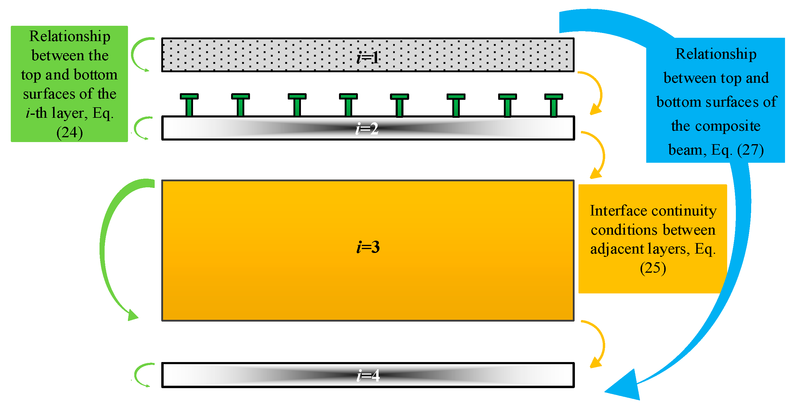
Figure 4 shows a schematic illustration of the transfer matrix principle. According to the known surficial load condition, the unknown parts in $R_m^1(0)$ are determined as below:

$$\left[\begin{array}{c}{u}_m^1(0)\\ v_m^1(0)\end{array}\right]=-{\left[\begin{array}{cc}{D}_{mp}^{31}(H)& D_{mp}^{32}(H)\\ D_{mp}^{41}(H)& D_{mp}^{42}(H)\end{array}\right]}^{-1}\left[\begin{array}{c}{E}_{mp}^3(H)\\ E_{mp}^4(H)\end{array}\right]-{\left[\begin{array}{cc}{D}_{mp}^{31}(H)& D_{mp}^{32}(H)\\ D_{mp}^{41}(H)& D_{mp}^{42}(H)\end{array}\right]}^{-1}\left[\begin{array}{cc}{D}_{mp}^{33}(H)& D_{mp}^{34}(H)\\ D_{mp}^{43}(H)& D_{mp}^{44}(H)\end{array}\right]\left[\begin{array}{c}-q_m\\ 0\end{array}\right],$$

(29)

where q_m can represent either a distributed load or a equivalent concentrated load,

$$q_m=\left\{\begin{array}{c}\frac{2}{L}{\displaystyle {\int }_0^{L}q(x)\sin ({\beta }_{m}x)dx, \mathit{for} \mathit{distributed} \mathit{load}}\\ \frac{2}{L}{\displaystyle {\int }_{a-0.5\Delta L}^{a+0.5\Delta L}\frac{P}{\Delta L}\sin ({\beta }_{m}x)dx, \mathit{for} \mathit{concentrated} \mathit{load} }\end{array}\right.,$$

P is a concentrated load, a is the coordinate of the concentrated load on the x-axis, and ΔL is the length of the small equivalent region. $D_{mi}^{\ast \ast }$ and $E_{mi}^{\ast \ast }$ are the elements of the matrices $D_m^i$ and $E_m^i$, respectively. Accordingly, $R_m^1(0)$ can be determined. Substituting $R_m^1(0)$ into Equations (25) and (27) gives the analytical solutions of stresses and displacements of the present composite I-beam with CSW.

2.4. Extension for Continuous Composite Beams

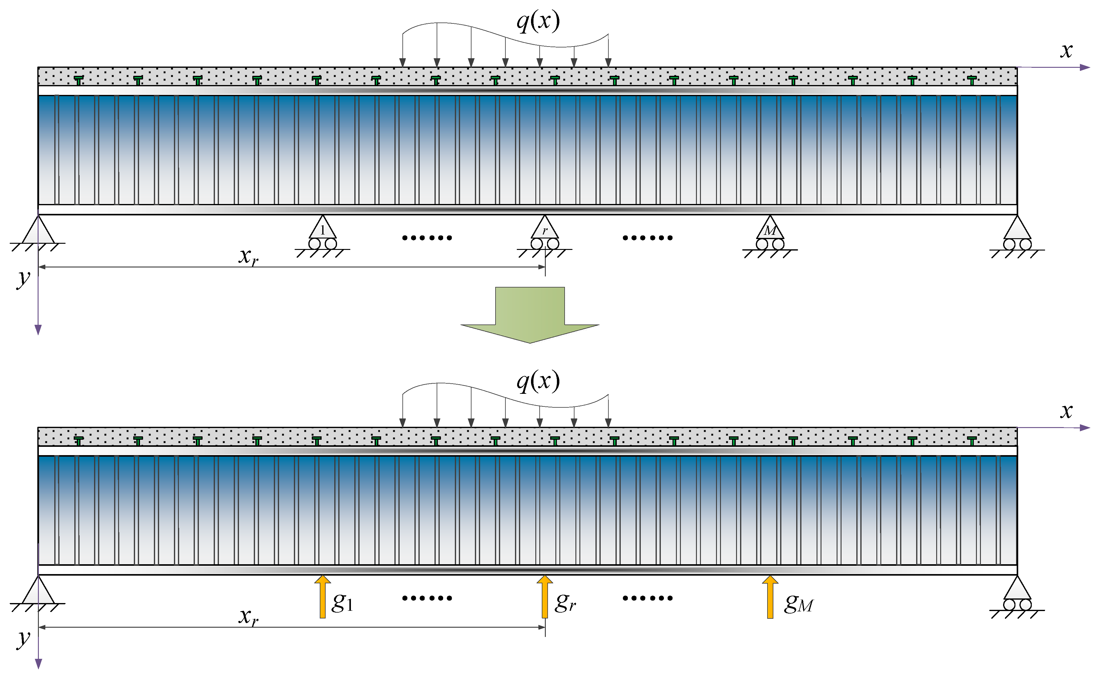
Based on the theoretical model of the simply supported composite I-beam with CSWs, the applicability of the proposed method to continuous beam systems is further discussed. Unless otherwise specified, the geometric parameters, material constants and load definitions of the continuous beam are consistent with those defined previously. As shown in Figure 5, the continuous composite I-beam with CSWs is supported by M supports along the bottom, and the position of the r-th support is denoted by x_r. The continuous composite beam can be regarded as the superposition of a single-span simply supported beam and a series of support reactions with unknown magnitudes. The reaction force at the r-th support is denoted by g_r.

Compared with the corresponding single-span simply supported composite beam, the continuous beam is subjected to a series of additional support reactions. Therefore, the surface loading condition can be rewritten as

$${\sigma }_y^1(x,0)=-q(x), {\tau }_{xy}^1(x,0)=0,$$

$${\sigma }_y^4(x_r,H)={\displaystyle {\sum }_{r=1}^M{g}_r\delta (x-x_r)}, {\tau }_{xy}^4(x,H)=0.$$

(30)

where $\delta (x)$ is the Dirac delta function, $\delta (x)=\left\{\begin{array}{c}\infty ,\hspace{0.33em}x=0\\ 0,x\ne 0 \end{array}\right.$, $\delta (x-x_r)$ denotes the position of the r-th support reaction, and g_k denotes the magnitude of the support reaction. Since the solutions of stresses and displacements for the simply supported case are expressed in Fourier series, the Dirac delta function is also expanded as

$$\delta (x-x_r)={\displaystyle \sum _{m=1}^{\infty }{w}_r^m}\sin ({\alpha }_{m}x), w_r^m={\displaystyle \frac{2}{L}}\sin ({\alpha }_m{x}_r).$$

(31)

The additional unknown variable can be determined by additional deformation compatibility condition at the r-th support:

$$v^4(x_r,H)=0 (r = 1, 2, \dots M),$$

(32)

The difference between the continuous beam and the single-span simply supported beam lies only in the additional support reactions at the bottom. Therefore, the relationship between the stresses and displacements at the top and bottom surfaces of the composite beam can still be determined by the transfer matrix method.

3. Example Analysis and Discussion

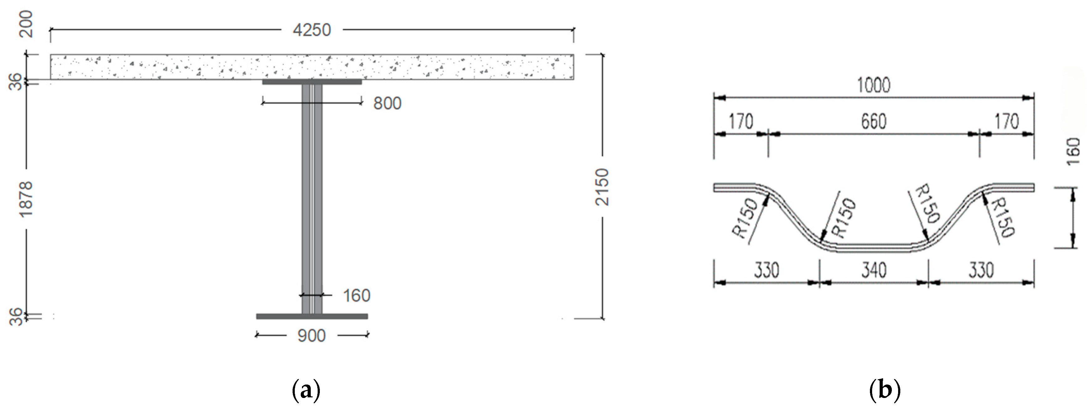
In this section, the proposed theoretical model for composite I-beams with corrugated steel webs under thermo-mechanical coupling is verified through comparative analyses, followed by parametric studies. Unless otherwise specified, the composite I-beam with CSWs from the Jiulong East Junction Bridge in China is adopted as the reference structure. The configuration and dimensions of the reference structure are shown in Figure 6. Its cross-sectional dimensions and material parameters are listed in

Table 1. Cross-sectional dimensions and material parameters of Jiulong East Junction Bridge.

	Cross-Sectional Dimensions (mm)	Material Parameters
Composite beam	b1 = 4250, b2 = 800, b3 = 160, b4 = 900,	Ec = 34.5 GPa, νc = 0.2, λc = 1.74 W/m/°C, αc = 1.1 × 10−5/°C,
	h1 = 200, h2 = 36, h3 = 1878, h4 = 36,	Es = 206 GPa, νs = 0.3, λs = 54 W/m/°C, αs = 1.2 × 10−5/°C
Corrugated steel web	a1 = 170, a2 = 160, tw = 12, θ = 45°	Ex = 0.0025 Es, Ey = 1.2 Es, Gxy = 0.83 Es, νyx =νs, νxy = 0.0021 νs, ${\alpha }_x^{AOP}$$= {\alpha }_y^{AOP}$ = 1.2 × 10−5/°C, ${\lambda }_y^{AOP}$$= 64.84 \mathrm{W}/\mathrm{m}/°\mathrm{C}, {\lambda }_z^{AOP}$ = 44.97 W/m/°C

, and the beam span is L = 45 m. The load applied on the upper surface of the composite beam is q(x) = 8 × 10³ N/m², and the ambient temperature is T_a = 20 °C, unless otherwise stated.

3.1. Comparison of Existing Results

The present solution is compared with the experimental results [13], the temperature distributions specified by China’s General Specifications for Design of Highway Bridges and Culverts (JTG D60-2015) [31], the American AASHTO LRFD Bridge Design Specifications, 8th Edition (AASHTO 2017) [32], and the German DIN-Fachbericht 101: Actions on Bridges (DIN 101) [33], as well as the finite element method (FEM) solution provided by ABAQUS. The research object is a steel–concrete composite bridge deck, and its cross-sectional dimensions and material parameters are taken from experiment [13], with two types of constraint conditions considered, namely single-span simply supported and multi -span continuous. The upper surface of the beam is only subjected to thermal action, without mechanical loads, and the ambient temperature is T_a = 9 °C. In the FEM model, the temperature field is modeled using DC2D4 elements with 598 elements in total, whereas the thermal stress and displacement are modeled using C3D8R elements with 26,112 elements in total. Recent machine-learning-based temperature prediction models have been discussed in the Introduction. Therefore, this section focuses on experimental results, FEM simulations and temperature distributions prescribed by design codes to validate the proposed analytical solution.

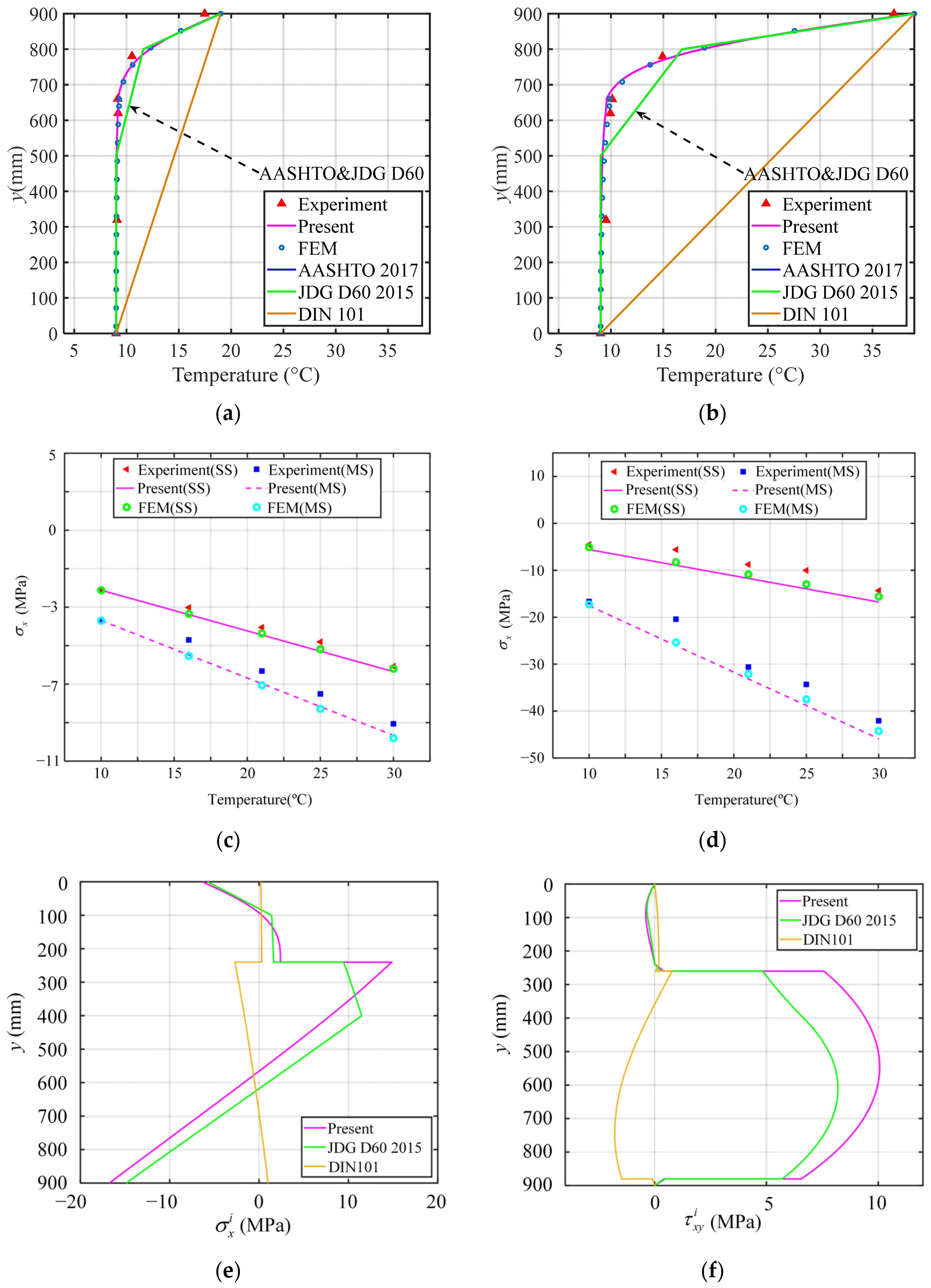
Figure 7 compares the temperature fields and thermal stresses obtained by different methods. It can be observed that (i) under different temperature conditions, the present solution agrees well with both the FEM and experimental results, with errors within 1.8% relative to the FEM results and within 9.5% relative to the experimental results, except for slight deviations near the shear connectors of the composite beam. (ii) Both JTG D60-2015 and AASHTO 2017 adopt multi-segment temperature distributions. Since the temperature measured at the bottom of the composite beam is equal to the ambient temperature, the temperature distributions given by two codes are identical. Relatively large errors are observed near the interface between the concrete slab and the steel I-beam, with a maximum error of 27.4%, whereas good agreement is obtained in the other regions. DIN 101 adopts a linear temperature distribution from the top to the bottom of the composite beam, which is relatively conservative, with a maximum error of 69.1%. (iii) The thermal stresses of the composite beam obtained from the present solution agree well with the experimental results, with a maximum error of 8.1%, while the FEM results are very close to the present solution, with an error of less than 2.1%. (iv) Although steel and concrete have relatively similar coefficients of thermal expansion, the non-uniform temperature field still induces thermal stresses in the composite beam. These stresses are much larger in the steel beam than in the concrete slab, and considerable shear stress is also generated in the web. (v) The thermal stresses obtained using JTG D60-2015 show good agreement with the present solution. Moreover, although the trilinear temperature distribution adopted by JTG D60-2015 results in a five-segment distribution of thermal normal stress σ_x, the shear stress varies smoothly within the web. (vi) The temperature field in JTG D60-2015 induces a thermal stress error of 23.3%, whereas DIN 101 leads to a much larger error.

3.2. Decoupling Analysis

For the thermo-mechanical coupling response, a conventional approach is to first evaluate the temperature-induced effect and the load-induced effect separately, and then combine them according to the superposition principle. However, the elastic modulus of steel degrades at elevated temperatures, and the corresponding reduction factor is given by [34]

$$E_T/E=1.02-0.035e^{T/280},$$

(33)

where 20 °C ≤ T ≤ 800 °C. The reduction factor in Equation (33) is used to characterize the degradation of the steel elastic modulus under thermal action. The present high-temperature analysis mainly focuses on the influence of elastic-modulus reduction on the thermo-mechanical coupling superposition relationship. The possible non-uniform degradation caused by one-sided high-temperature exposure of the web is not further considered, which would require a more refined three-dimensional temperature field and three-dimensional thermoelastic analysis.

To verify whether the superposition principle remains valid at elevated temperatures, the stresses and displacements of the composite beam were investigated under four loading cases: pure mechanical (PM), pure thermal (PT), mechanical-thermal (MT) and PM2. Here, PM2 denotes a modified PM case in which the temperature-induced degradation of the elastic modulus is considered, whereas thermal expansion deformation is not included. The definitions of these four loading cases are given in

Table 2. Definition of the four analysis cases. Note: the symbol ✓ indicates that the corresponding effect is considered in the analysis case.

Case	Stress and Deformation Induced by Mechanical Loading	Stress and Deformation Induced by Temperature	Temperature-Induced Degradation of Elastic Modulus
PM	✓
PM2	✓		✓
PT		✓	✓
MT	✓	✓	✓

.

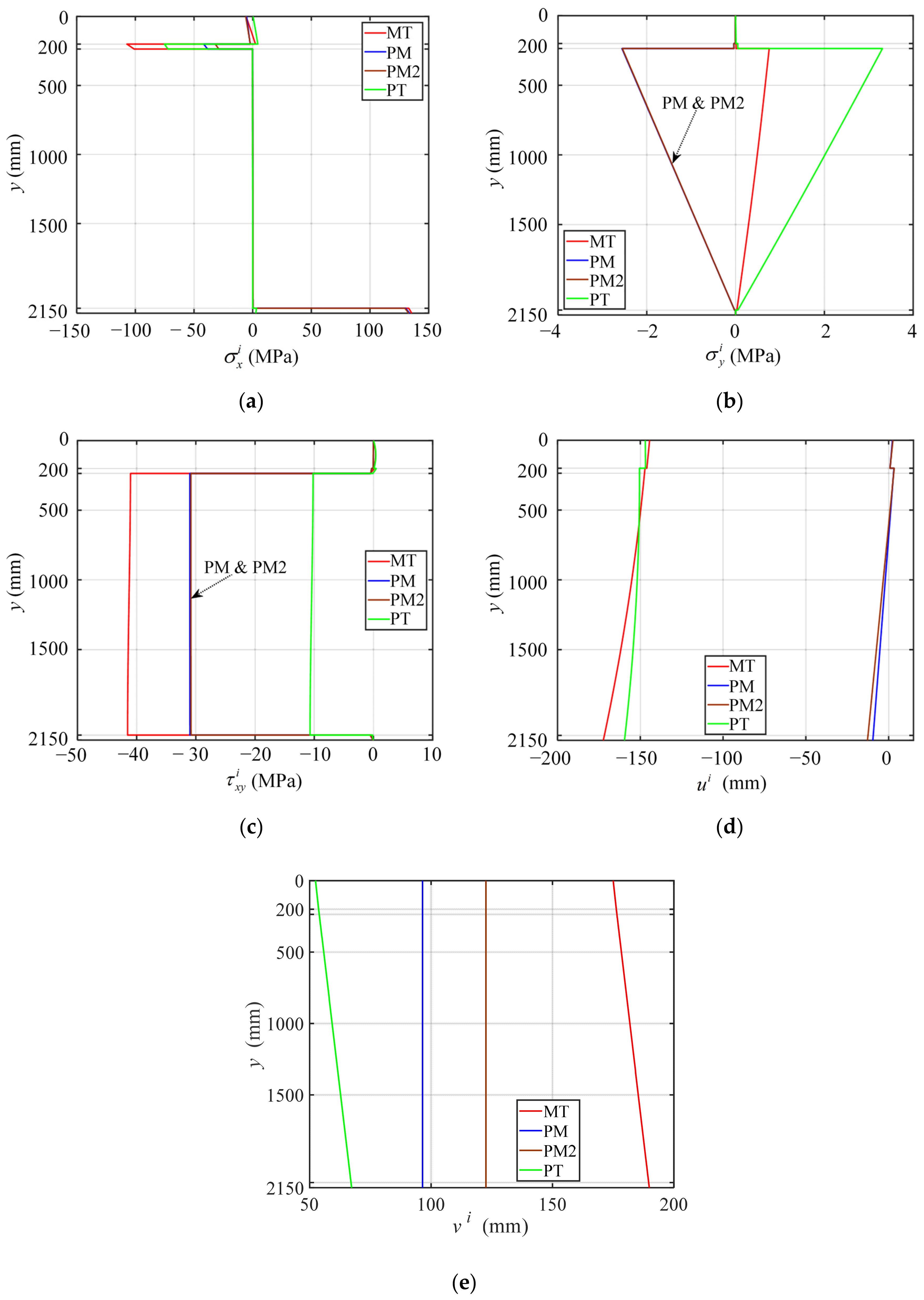
Figure 8 illustrates the through-thickness distributions of stress and displacement in the composite beam under four analytical cases. In these cases, the applied load on the top surface of the composite beam is q = 8 × 10³ N/m², the interfacial shear stiffness is 100 MPa, and the beam is subjected to a uniform thermal environment of T = 600 °C. From the figure, it can be observed that (i) under the PT and PM cases, the directions of stress and displacement are the same except for σ_y. The relatively larger bending deformation of the steel I-beam is restrained by the concrete slab, which undergoes smaller deformation, thereby resulting in tensile stress, that is, a negative σ_y. (ii) The maximum normal stress induced by the external load occurs at the bottom flange of the steel I-beam, whereas the maximum stress induced by temperature appears in the flange region of the steel beam. This is because the concrete slab and the steel beam jointly resist the bending deformation caused by the external load, while thermal stress is induced by the difference in thermal expansion deformation between steel and concrete, with the maximum value occurring near their interface. (iii) The shear stress in the composite beam is caused by the difference in thermal expansion deformation between steel and concrete as well as by the composite action, and its magnitude is relatively smaller than that induced by the external load. The displacement u caused by temperature is much greater than that caused by the external load, whereas the displacement v caused by temperature is much smaller than that caused by the external load, mainly because the length of the composite beam is much greater than its height. (iv) At elevated temperatures, the mechanical behavior of the composite beam no longer strictly follows the conventional superposition principle. Instead, the load-induced mechanical response should be evaluated by considering the temperature-induced degradation of the elastic modulus simultaneously, which can be expressed as

MT ≠ PM + PT,

(34)

MT = PM2 + PT,

(35)

where the former and latter equations represent the conventional superposition principle and the modified superposition principle proposed in this study, respectively.

3.3. Effects of Interfacial Shear Stiffness

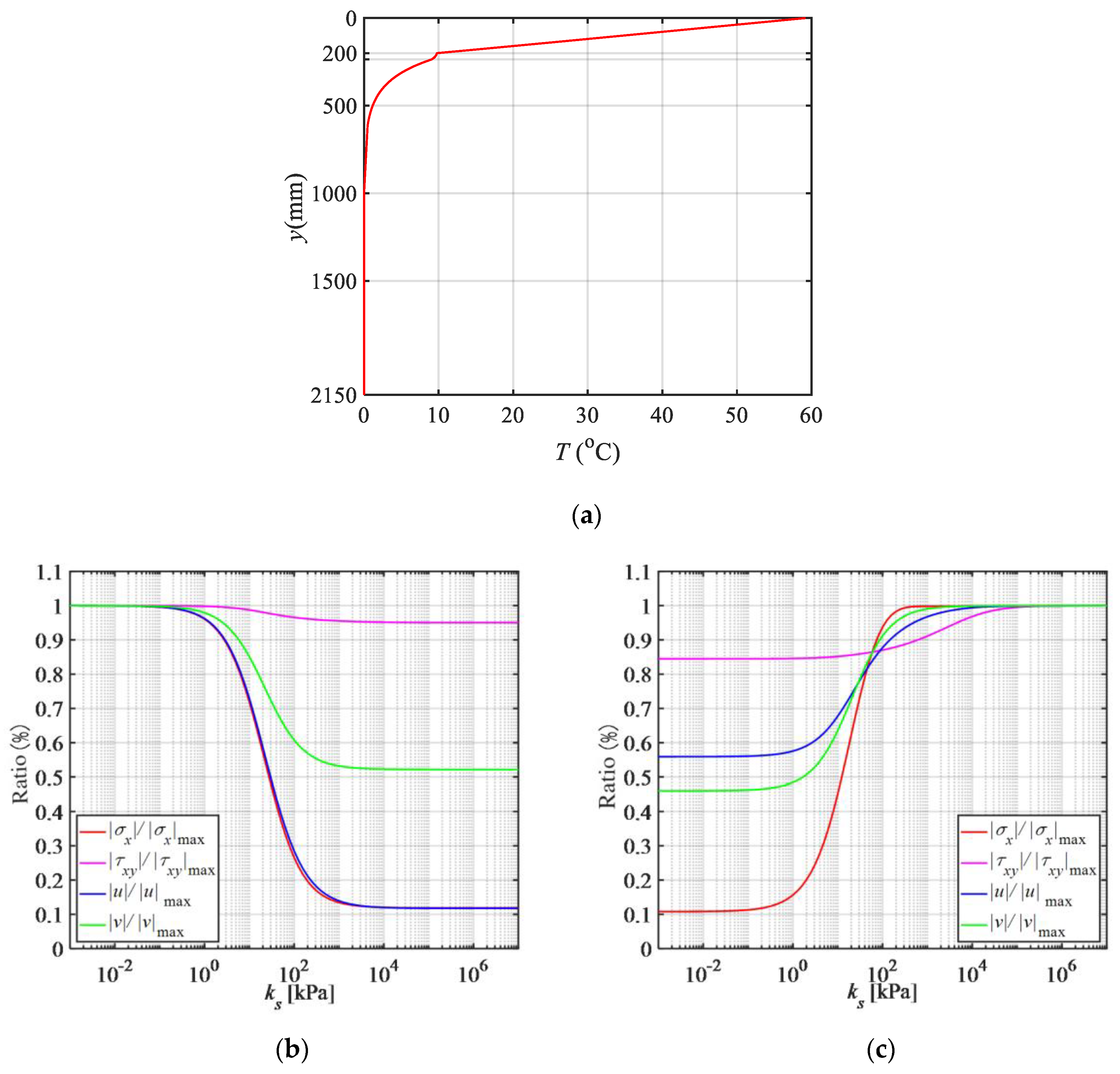
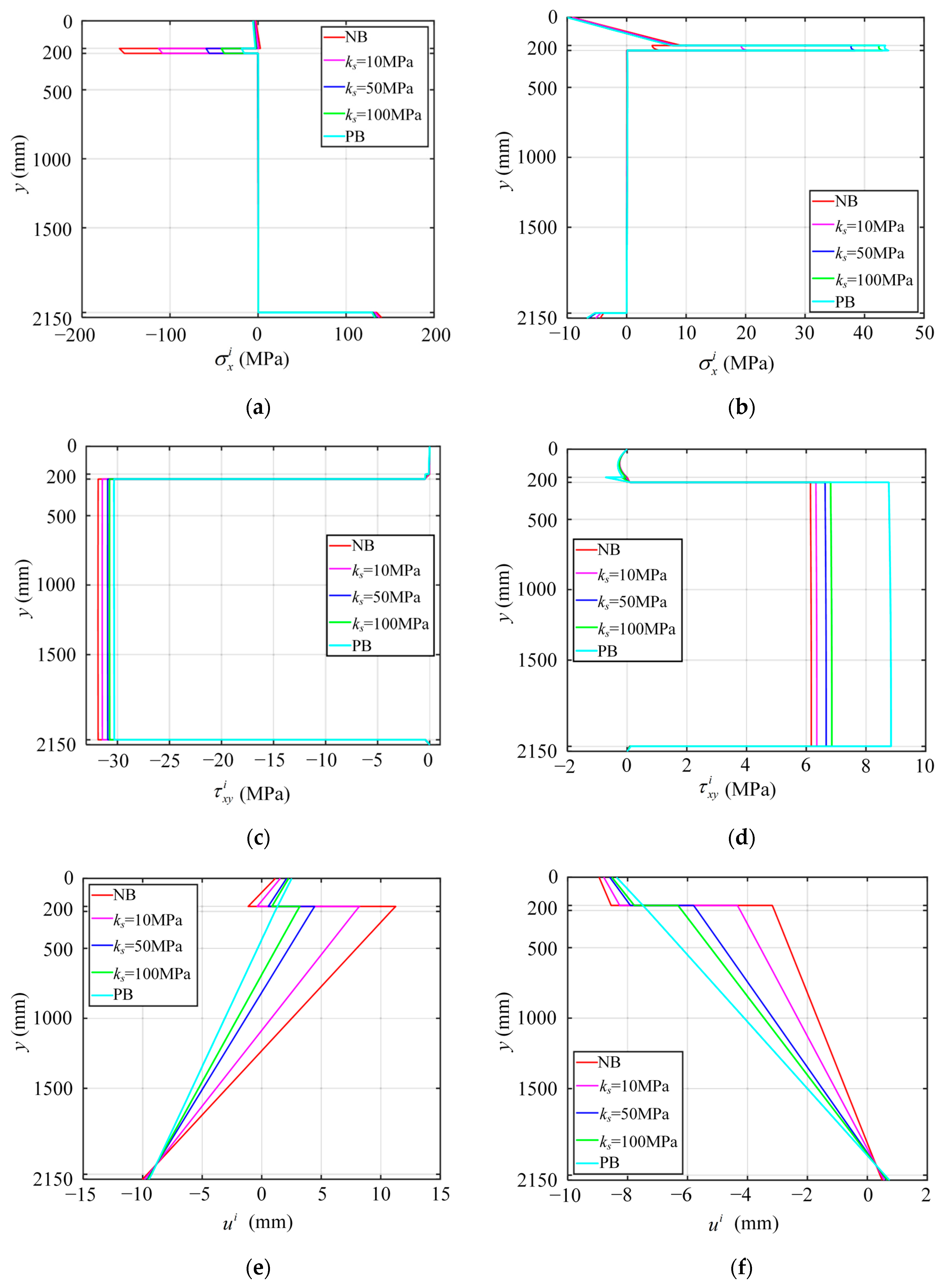
To investigate the influence of the interfacial shear stiffness k_s on the mechanical behavior of the composite beam under combined thermal and mechanical loading, the mechanical effect and the thermal effect are examined separately in this section based on the modified superposition principle proposed above. A temperature of 80 °C is applied to the upper surface of the composite beam, while the remaining surfaces are subjected to convective heat transfer with air, with a convective heat transfer coefficient of β = 20 W/m²∙°C. Figure 9 and Figure 10 present the steady-state temperature distribution of the composite beam and the effects of interfacial shear stiffness on the stresses and displacements. Here, PB and NB denote the perfectly bonded interface and the unbonded interface, respectively.

It can be seen from these figures that (i) under the PM2 analytical case, the stress and displacement generally decrease with increasing k_s, and remain almost unchanged when k_s > 10⁴ MPa or k_s < 10⁻² MPa, which correspond to rigid interfacial connection and no interfacial connection, respectively. In contrast, under the PT analytical case, the stress and displacement generally increase with increasing k_s, and the corresponding thresholds for rigid interfacial connection and no interfacial connection are k_s > 10⁶ MPa and k_s < 10⁻² MPa, respectively. This difference arises because a larger k_s enhances the overall flexural stiffness of the composite beam, thereby reducing the stress and displacement induced by external loading. In the case of thermal effects, however, a larger k_s imposes stronger restraint on the thermal deformation of the concrete slab and the steel I-beam, resulting in higher thermal stresses. Moreover, because the temperature decreases non-uniformly from the top to the bottom of the composite beam, both the concrete slab and the steel I-beam tend to bend upward. As k_s increases, the composite action becomes stronger, and the overall upward bending deformation correspondingly increases. (ii) Under the PM2 case, σ_x and u are the most sensitive to k_s, whereas τ_xy is the least affected. Under the PT case, σ_x is most sensitive to k_s, followed by u, while τ_xy remains the least sensitive. (iii) The composite beam bends downward under external loading but upward under the considered non-uniform temperature distribution. As a result, the directions of stress and displacement in the two analytical cases are opposite, and their effects can therefore partially counteract each other.

3.4. Temperature Effect Mitigation by Thermal Insulation

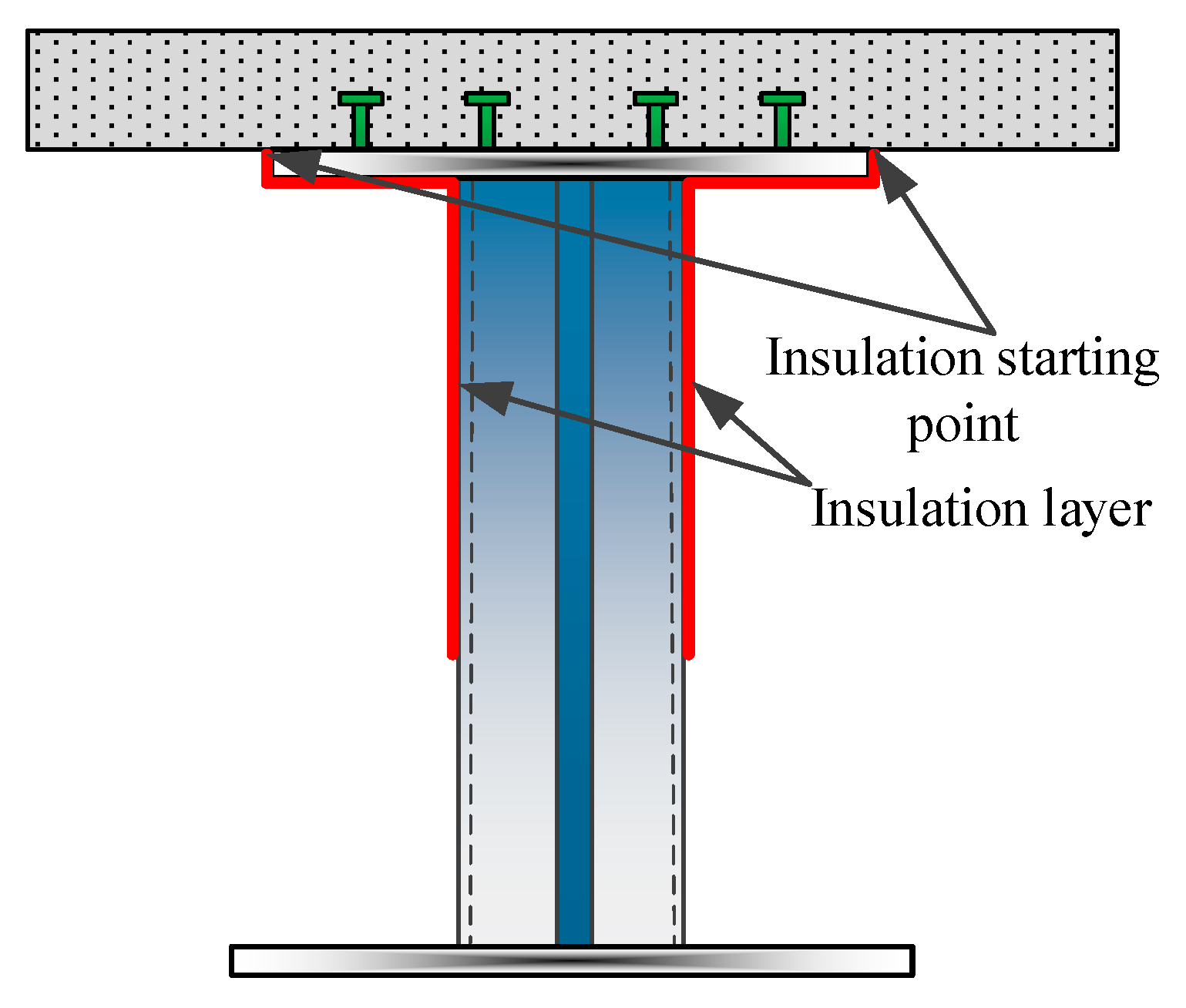
Since steel has a lower specific heat capacity and a higher thermal conductivity, the steel I-beam dissipates heat rapidly. By contrast, concrete has a higher specific heat capacity and a lower thermal conductivity, and therefore the concrete slab dissipates heat more slowly. This difference in heat dissipation capacity leads to a large temperature gradient in the vicinity of the concrete slab-steel I-beam interface. To reduce this temperature gradient and mitigate the resulting thermal stresses, an insulation layer can be applied to the side surfaces of the composite beam, as illustrated in Figure 11.

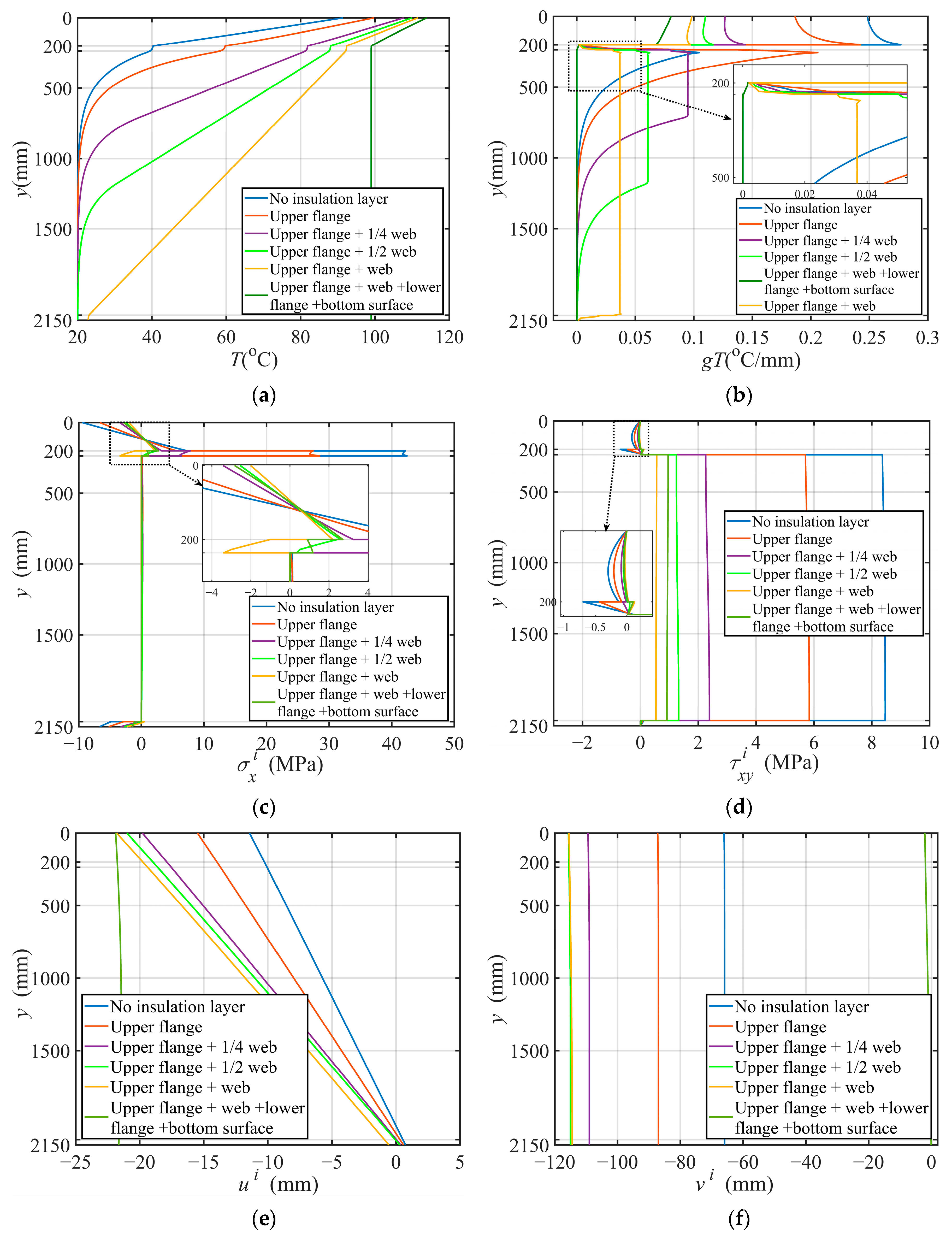
Considering that the upper surface of the composite beam is subjected to continuous solar radiation with an intensity of 1000 W/m², and that the thermal boundary condition at the insulation layer is adiabatic. Figure 12a,b present the effects of different insulation schemes on the steady-state temperature distribution of the composite beam, where g_T denotes the temperature gradient. The results indicate that, under the full-coverage insulation scheme for the I-beam, the temperature within the steel beam is nearly uniformly distributed. For all other schemes, the temperature at the bottom of the steel beam remains close to the ambient temperature. In the absence of insulation, the largest temperature gradient occurs in the vicinity of the interface between the concrete slab and the I-beam. Furthermore, the corresponding thermal stresses and displacements of the composite beam under different insulation layouts are shown in Figure 12c–f. The figure shows that (i) compared with the case without thermal insulation, the maximum thermal stresses σ_x and τ_xy are reduced by 81.5% and 72.3%, respectively, when the insulation scheme covering the upper flange and one-quarter of the web of the steel I-beam is adopted. (ii) Since the temperature is higher at the top of the composite beam and lower at the bottom, the thermal displacement u exhibits a distribution pattern characterized by larger values at the top and smaller values at the bottom. Because the coefficients of thermal expansion of steel and concrete are similar, the composite beam bends upward under this non-uniform temperature field. (iii) Under the full insulation scheme for the steel I-beam, the thermal displacement v of the composite beam is nearly zero, representing a reduction of 96.8% compared with the case without insulation. This indicates that the composite beam hardly bends upward under thermal action, mainly because the temperature field becomes approximately uniform under this insulation scheme.

4. Conclusions

An analytical framework for simply supported composite I-beams with CSW under thermo-mechanical coupling is developed in this study. The two-dimensional steady-state temperature field of the cross-section is obtained using the finite difference method. Based on thermoelastic theory, the analytical solutions for stresses and displacements are derived using the eigenvalue method and the transfer matrix method. The main conclusions are as follows:

• The proposed method correlates well with the measured experimental results, with a maximum error of 9.5%, and exhibits satisfactory consistency with finite element simulations, where the error is less than 2.1%. In comparison with mainstream design codes, JTG D60-2015 and AASHTO 2017 yield reasonable predictions, while DIN 101 produces considerably larger errors.
• The results reveal that the traditional superposition principle exhibits substantial inaccuracy under high-temperature conditions. By incorporating the temperature-dependent degradation of elastic modulus in PM service scenarios, the modified superposition principle proposed in this work can better describe the thermo-mechanical coupling response.
• The interfacial shear stiffness has a significant influence on the stresses and displacements of the composite beam within a certain range. Under mechanical loading, the stresses and displacements generally decrease with increasing interfacial stiffness, whereas under thermal loading they generally increase. Among the considered response quantities, the normal stress σ_x and the displacement u are the most sensitive to the interfacial stiffness, while the shear stress τ_xy is the least affected.
• Side-surface insulation of the steel I-beam effectively reduces the temperature gradient and mitigates the associated thermal effects. In particular, partial insulation of the upper flange and web markedly reduces the thermal stresses, whereas full insulation makes the temperature field nearly uniform and significantly suppresses the upward bending deformation of the composite beam.
• The present comparison is based on a selected bridge case from the Jiulong East Junction Bridge. Although good agreement is obtained among the present solution, experimental results and finite element simulations, more composite I-beam spans with CSWs and different geometric parameters should be examined in future studies to further verify the general applicability of the proposed method.

References

1. He, J.; Liu, Y.; Chen, A.; Yoda, T. Mechanical behavior and analysis of composite bridges with corrugated steel webs: State-of-the-art. Int. J. Steel Struct. 2012, 12, 321–338. [Google Scholar] [CrossRef]
2. Jiang, R.J.; Kwong Au, F.T.; Xiao, Y.F. Prestressed Concrete Girder Bridges with Corrugated Steel Webs: Review. J. Struct. Eng. 2015, 141, 04014108. [Google Scholar] [CrossRef]
3. He, J.; Wang, S.; Liu, Y.; Dai, L.; Lyu, Z.; Li, C.; Xin, H.; Tan, C. The development of composite bridges with corrugated steel webs in China. Proc. Inst. Civ. Eng.-Bridge Eng. 2021, 174, 28–44. [Google Scholar] [CrossRef]
4. Li, L.; Chen, B.; Zhou, L.; Xia, Q.; Zhou, Y.; Zhou, X.; Xia, Y. Thermal behaviors of bridges—A literature review. Adv. Struct. Eng. 2023, 26, 985–1010. [Google Scholar] [CrossRef]
5. He, J.; Liu, Y.; Chen, A.; Wang, D.; Yoda, T. Bending behavior of concrete-encased composite I-girder with corrugated steel web. Thin-Walled Struct. 2014, 74, 70–84. [Google Scholar] [CrossRef]
6. Liu, X.-G.; Fan, J.-S.; Nie, J.-G.; Bai, Y.; Han, Y.; Wu, W. Experimental and analytical studies of prestressed concrete girders with corrugated steel webs. Mater. Struct. 2015, 48, 2505–2520. [Google Scholar] [CrossRef]
7. Nawar, M.T.; El-Zohairy, A.; Maaly, H.M.; Husain, M.; Salama, I.; Mousa, E. Prestressed Steel-Concrete Composite I-Beams with Single and Double Corrugated Web. Buildings 2023, 13, 647. [Google Scholar] [CrossRef]
8. Bi, Z.; Yang, G. Shear strength of steel-concrete composite I-beams with corrugated steel webs. Structures 2024, 69, 107317. [Google Scholar] [CrossRef]
9. Zha, S.; Deng, W.; Liu, D.; Zhang, J.; Gu, J. Experimental study on flexural behavior of steel-laminated concrete (NC and UHPC) composite beams with corrugated steel webs. Eng. Struct. 2024, 306, 117802. [Google Scholar] [CrossRef]
10. Abbas, H.H.; Sause, R.; Driver, R.G. Analysis of Flange Transverse Bending of Corrugated Web I-Girders Under In-Plane Loads. J. Struct. Eng. 2007, 133, 347–355. [Google Scholar] [CrossRef]
11. Ma, H.; Liu, X.; Yao, C.; Cao, Y. Research in the Temperature Effect of Corrugated Steel Webs Combined Bridge. In Proceedings of the 5th International Conference on Civil Engineering and Transportation 2015; Atlantis Press: Paris, France, 2015. [Google Scholar] [CrossRef][Green Version]
12. Huang, S.; Cai, C.; He, X.; Li, C. Comparison of the corrugated steel web composite box-girder and traditional girders regarding temperature field under solar radiation. Eng. Struct. 2023, 291, 116419. [Google Scholar] [CrossRef]
13. Wang, D.; Tan, B.; Wang, X.; Zhang, Z. Experimental study and numerical simulation of temperature gradient effect for steel-concrete composite bridge deck. Meas. Control 2021, 54, 681–691. [Google Scholar] [CrossRef]
14. Fan, J.-S.; Liu, Y.-F.; Liu, C. Experiment study and refined modeling of temperature field of steel-concrete composite beam bridges. Eng. Struct. 2021, 240, 112350. [Google Scholar] [CrossRef]
15. Li, H.; Zhang, Z.; Deng, N. Temperature Field and Gradient Effect of a Steel-Concrete Composite Box Girder Bridge. Adv. Mater. Sci. Eng. 2021, 2021, 9901801. [Google Scholar] [CrossRef]
16. Zhang, H.; Long, H.; Chen, F.; Luo, Y.; Xiao, X.; Deng, Y.; Lu, N.; Liu, Y. Temperature field prediction for a PC beam bridge with corrugated steel webs using BP neural network and measured data. Structures 2024, 68, 107232. [Google Scholar] [CrossRef]
17. Zhang, H.; Long, H.; Chen, F.; Luo, Y.; Xiao, X.; Deng, Y.; Lu, N.; Liu, Y. Temperature gradient model of PC beams with corrugated steel webs in China using random forest algorithm and 50 years meteorological monitoring data. Structures 2025, 80, 109781. [Google Scholar] [CrossRef]
18. Shan, C.; Liu, W. Temperature stress analysis of prestressed concrete box girder with corrugated steel webs. Trans. Tianjin Univ. 2012, 18, 97–103. [Google Scholar] [CrossRef]
19. Fan, J.-S.; Li, B.-L.; Liu, C.; Liu, Y.-F. An efficient model for simulation of temperature field of steel-concrete composite beam bridges. Structures 2022, 43, 1868–1880. [Google Scholar] [CrossRef]
20. Xiang, W.; Zhang, H.; Zheng, Z.; Ding, J.; Zhao, Q. Study on Temperature Effect and Calculation Method of Steel-Concrete Composite Bridge. J. Phys. Conf. Ser. 2023, 2476, 012040. [Google Scholar] [CrossRef]
21. Cai, M.; Liu, S.; Wang, F. Temperature Effect of Composite Girders with Corrugated Steel Webs Considering Local Longitudinal Stiffness of Webs. Buildings 2024, 14, 1939. [Google Scholar] [CrossRef]
22. Wang, R.; Ji, W.; Li, X.; Peng, K.; Peng, C.; Wang, C. Thermal load models for the static design of steel-concrete composite girders. Structures 2023, 51, 1004–1018. [Google Scholar] [CrossRef]
23. Peng, X.; Zhou, M.; Wang, Y. Stress distribution in composite girders with flat and corrugated steel webs under temperature gradient. Thin-Walled Struct. 2025, 216, 113667. [Google Scholar] [CrossRef]
24. Chen, F.; Tan, B.; Tang, H.; Zhang, H.; Luo, Y.; Xiao, X.; Liu, Y.; Lu, N. An interpretable random forest surrogate for rapid SIF prediction and fatigue life assessment of double-sided U-rib welds in orthotropic steel decks. Eng. Fail. Anal. 2026, 187, 110582. [Google Scholar] [CrossRef]
25. Zhang, H.; Zhao, L.; Chen, F.; Luo, Y.; Xiao, X.; Liu, Y.; Deng, Y. A machine learning and multi-source authentic data-driven framework for accurate fatigue life prediction of welds in existing steel bridge decks. Thin-Walled Struct. 2026, 222, 114559. [Google Scholar] [CrossRef]
26. Zhang, H.; Dong, Y.; Liu, H.; Liu, B.; Deng, Y. A novel multi-scale mechanical model for fatigue expansion of corroded high-strength steel wires. Constr. Build. Mater. 2026, 514, 145567. [Google Scholar] [CrossRef]
27. Xiao, X.; Tang, H.; Zhang, H.; Luo, Y.; Lu, N.; Liu, Y.; Chen, F. Bayesian optimization CNN-LSTM neural network for fatigue life prediction of Rib-to-deck Welds in orthotropic steel decks. Structures 2026, 84, 111088. [Google Scholar] [CrossRef]
28. Guan, B.; Xu, T.; Yue, K.; Deng, W.; Wu, P.; Zhang, J. Exact solution and case studies for composite I-beam with corrugated steel web. Case Stud. Constr. Mater. 2023, 19, e02422. [Google Scholar] [CrossRef]
29. Dissanayaka, M.P.; Yapa, H.D. Numerical prediction of early age concrete temperature via 3D finite difference simulation. J. Natl. Sci. Found. 2021, 49, 539. [Google Scholar] [CrossRef]
30. Zhang, Z.; Zhou, D.; Fang, H.; Zhang, J.; Li, X. Analysis of laminated beams with temperature-dependent material properties subjected to thermal and mechanical loads. Compos. Struct. 2019, 227, 111304. [Google Scholar] [CrossRef]
31. JTG D60-2015; General Specifications for Design of Highway Bridges and Culverts. China Communications Press: Beijing, China, 2015.
32. AASHTO 2017; AASHTO LRFD Bridge Design Specifications, 8th Edition. American Association of State Highway and Transportation Officials: Washington, DC, USA, 2017.
33. DIN-Fachbericht 101:2009-03; Actions on Bridges. Beuth Verlag: Berlin, Germany, 2009.
34. Wang, W.; Liu, B.; Kodur, V. Effect of Temperature on Strength and Elastic Modulus of High-Strength Steel. J. Mater. Civ. Eng. 2013, 25, 174–182. [Google Scholar] [CrossRef]
Figure 1. Simply supported composite I-beam with CSW. Note: L is the beam span, H is the total height, q(x) is the external load, Tu is the top surface temperature, Ta is the ambient temperature. hi and bi are the height and width of each layer, C is the width of CSW, tw is the web thickness, and a1, a2 and a3 are the corrugation geometric parameters.
Buildings 16 02142 g001
Figure 2. Schematic diagram for equivalent thermal coefficients of CSW. Note: The red and blue arrows indicate heat input and heat output, respectively, and are used to illustrate the heat-transfer direction in the thermal-conductivity equivalence.
Buildings 16 02142 g002
Figure 3. Schematic diagram of finite difference grid of composite I-beam.
Buildings 16 02142 g003
Figure 4. Schematic of the transfer matrix method.
Buildings 16 02142 g004
Figure 5. Schematic diagram of support equivalence for a continuous composite beam.
Buildings 16 02142 g005
Figure 6. A diagram of the composite I-beam with CSWs from the Jiulong East Junction Bridge: (a) cross-sectional dimensions; (b) corrugation geometry and dimensions of the CSW.
Buildings 16 02142 g006
Figure 7. Comparison of temperature fields and thermal stresses: (a) T = 19 °C; (b) T = 39 °C; (c) Maximum σx in the concrete slab; (d) Maximum σx in the steel beam; (e) Thermal stress σx; (f) Thermal shear stress τxy. Note: MS, multi-span; SS, single-span.
Buildings 16 02142 g007
Figure 8. Through-thickness distributions of stresses and displacements in the composite beam under four analysis cases. (a) σ x i at x = L/2; (b) σ y i at x = L/2; (c) τ x y i at x = 0; (d) ui at x = 0; (e) vi at x = L/2.
Buildings 16 02142 g008
Figure 9. Effects of interfacial shear stiffness on the maximum stresses and displacements of the composite beam. (a) Temperature distribution of the composite beam with respect to Ta; (b) Effect of ks on PM2; (c) Effect of ks on PT.
Buildings 16 02142 g009
Figure 10. Effects of interfacial shear stiffness on the stress and displacement distributions of the composite beam. (a) σ x i at x = L/2 on PM2; (b) σ x i at x = L/2 on PT; (c) τ x y i at x = 0 on PM2; (d) τ x y i at x = 0 on PT; (e) ui at x = 0 on PM2; (f) ui at x = 0 on PT.
Buildings 16 02142 g010
Figure 11. Schematic of side insulation of the steel I-beam.
Buildings 16 02142 g011
Figure 12. Effects of side insulation of the steel I-beam on the temperature, thermal stress and displacement of the composite beam. (a) Temperature distribution; (b) Temperature gradient distribution; (c) σ x i at x = L/2; (d) τ x y i at x = 0; (e) ui at x = 0; (f) vi at x = L/2.
Buildings 16 02142 g012