Evaluating State-of-the-Art Models for the Seismic Response of RC Core Walls with Torsion

Abstract

Reinforced concrete core walls serve as the primary lateral load-resisting system in mid- and high-rise buildings, providing stability against wind and earthquake forces. Many of these walls feature non-planar cross-sections that lead to complex deformation modes, which require discretizing the wall segments for accurate numerical simulation. This paper investigates the dynamic response of U-shaped RC core walls using state-of-the-practice micro- and macroscopic modeling techniques, namely: Three-dimensional solid elements, nonlinear Beam-Truss Models, the force–displacement version of the Multiple-Vertical-Line-Element-Model, and the Applied Element Method. These models are validated against newly obtained large-scale shake table test data, assessing both global and local structural responses. Key parameters, including displacements, shear forces, rotations, torque, strain distributions, and shear deformations, are analyzed to refine numerical modeling approaches. Findings highlight some of the limitations of the different modeling approaches and provide best-practice recommendations for engineers to improve predictive accuracy. This study advances the understanding of non-planar RC wall behavior, aiding in the development of more reliable seismic design methodologies.

1. Introduction

Reinforced concrete (RC) core walls are the primary lateral load-resisting system for mid- and high-rise buildings worldwide, safeguarding structures against strong wind and earthquake forces. These walls typically have non-planar cross-sections, offering engineers and architects an efficient solution for achieving lateral strength and stiffness in multiple directions [1], resisting torsional actions [2,3], accommodating elevators, stairs, and service ducts [4], and meeting fireproofing requirements. Given their critical structural role, accurate seismic modeling and simulation are essential to predict key design and assessment engineering parameters, such as bending moments, shear stresses, global displacements, interstory drifts, and local strains.

Due to its simplicity and low computational demands [5], a commonly used method in engineering practice for modeling RC walls employs one-dimensional beam elements where the entire cross-section is assigned to a single stick model [6]. While this approach can be, under specific assumptions, appropriate for planar (rectangular) walls, it is inadequate for non-planar sections. Among others, a major limitation is the inability of typical beam elements to capture warping deformations [7], which are particularly significant for certain non-planar configurations, such as U-shaped walls under torsional loading. Additionally, non-planar walls usually experience larger shear deformations than their planar counterparts [1,8], and beam elements cannot accurately simulate the distribution of shear forces between webs and flanges [9]. These limitations highlight the need for alternative numerical modeling approaches capable of capturing the coupled axial–flexural–torsional behavior of non-planar RC core walls.

This paper employs and compares state-of-the-art micro- and macroscopic modeling approaches to simulate the seismic response of RC U-shaped core walls. Specifically, it uses solid finite elements (FEs) for three-dimensional structures with VecTor3; a combination of beam and truss elements in the Beam-Truss Model (BTM); advanced beam-column elements in the force–displacement version of the Multiple-Vertical-Line-Element-Model (MVLEM-FD); and the Applied Element Method (AEM), which merges the strengths of continuous FE formulations with the advantages of discrete element methods. Their effectiveness is assessed using newly obtained experimental data from large-scale shake table tests, with a focus on both global and local responses. Beyond evaluating these modeling approaches, this study also provides best-practice recommendations to help engineers gain greater confidence in simulation results.

2. Research Significance

A recent study compared several state-of-the-art numerical modeling approaches for simulating planar RC walls tested using a quasi-static approach [10]. The present research builds on this work by applying similar methodologies to non-planar (U-shaped) walls using nonlinear dynamic response history analyses. This investigation is made possible by a recent experimental campaign involving dynamic testing of core walls [11], which has yielded a comprehensive dataset for evaluating flexural and torsional behavior. Despite torsion being an inevitable effect in buildings subjected to earthquake ground motions [12], little research has focused on how core walls—the primary structural system resisting such torsional demands—perform under combined axial–flexural–torsional loading.

It is worth noting that the same experimental test unit used in this study served as the basis for the ERIES-ALL4WALL blind prediction competition [13]. That competition focused primarily on the dynamic response of the wall, asking participants to estimate failure modes and maximum engineering demand parameters—including relative horizontal displacements, inertial forces, and tensile strains at the base—prior to the full dataset becoming available. A total of 24 predictions were submitted using a wide range of software and modeling approaches, as summarized in Hoult and Almeida [14]. The present study differs from that competition in two important respects. First, this is a post-diction study: the full experimental dataset is now available, enabling more rigorous and detailed comparisons between numerical results and measured response. Second, the four modelling approaches examined here were not among those used in the competition, meaning this work extends the state-of-knowledge beyond what was captured in the blind predictions. Together, these distinctions clarify the novel contribution of the present study relative to prior comparative work on this test unit.

3. Experimental Data Used for Model Evaluation

The ERIES-ALL4WALL project [15] conducted shake-table tests on two slender U-shaped walls: one reinforced with steel and the other with iron-based shape memory alloy rebars. The present study focuses on the first steel-reinforced unit, UWS1. To the authors’ knowledge, these tests were the first to assess the nonlinear torsional response of U-shaped core walls under dynamic loading. The project has been extensively documented in previous works [11], detailing the test setup, wall design, instrumentation, and ground motion selection. For brevity, only a summary of unit UWS1 is provided here.

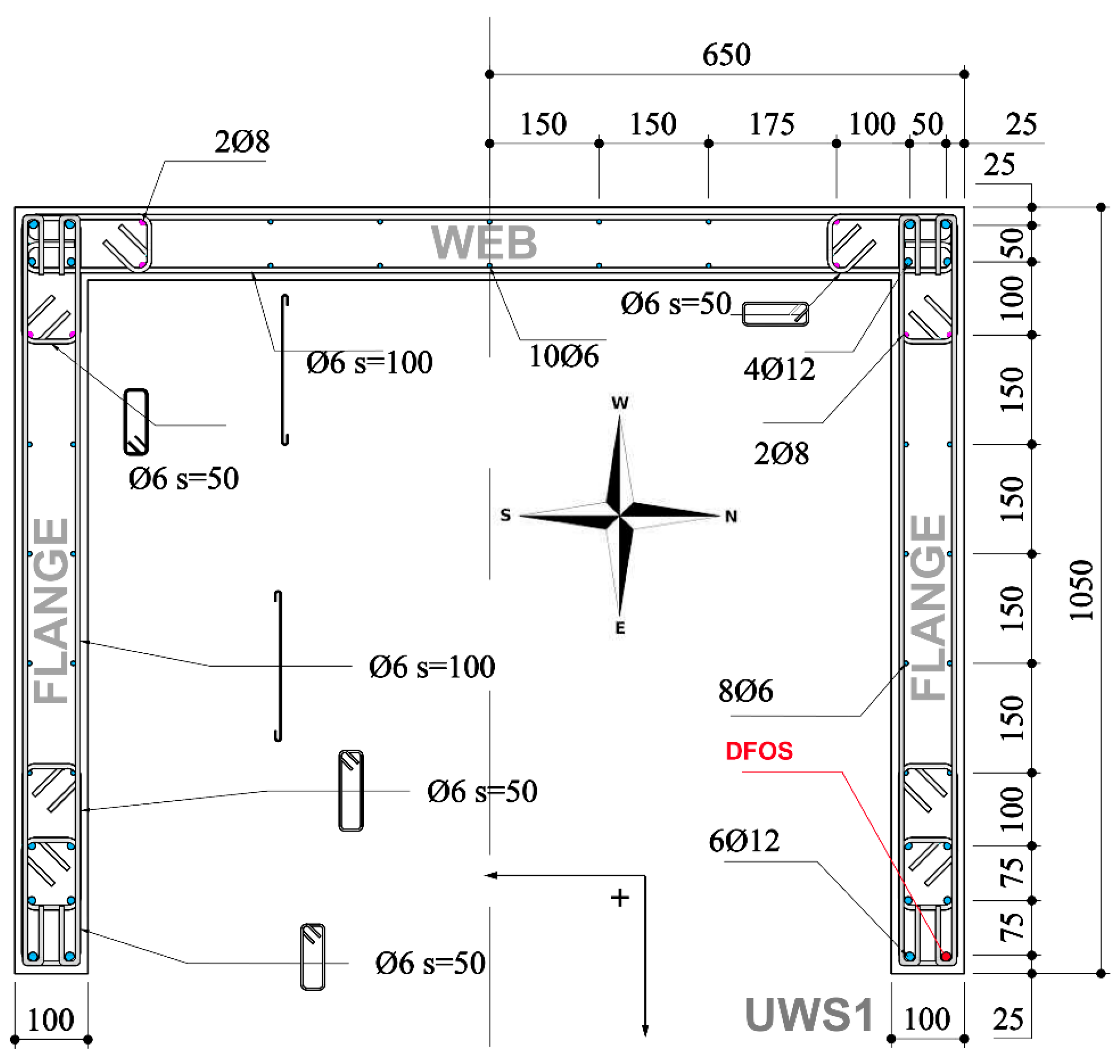
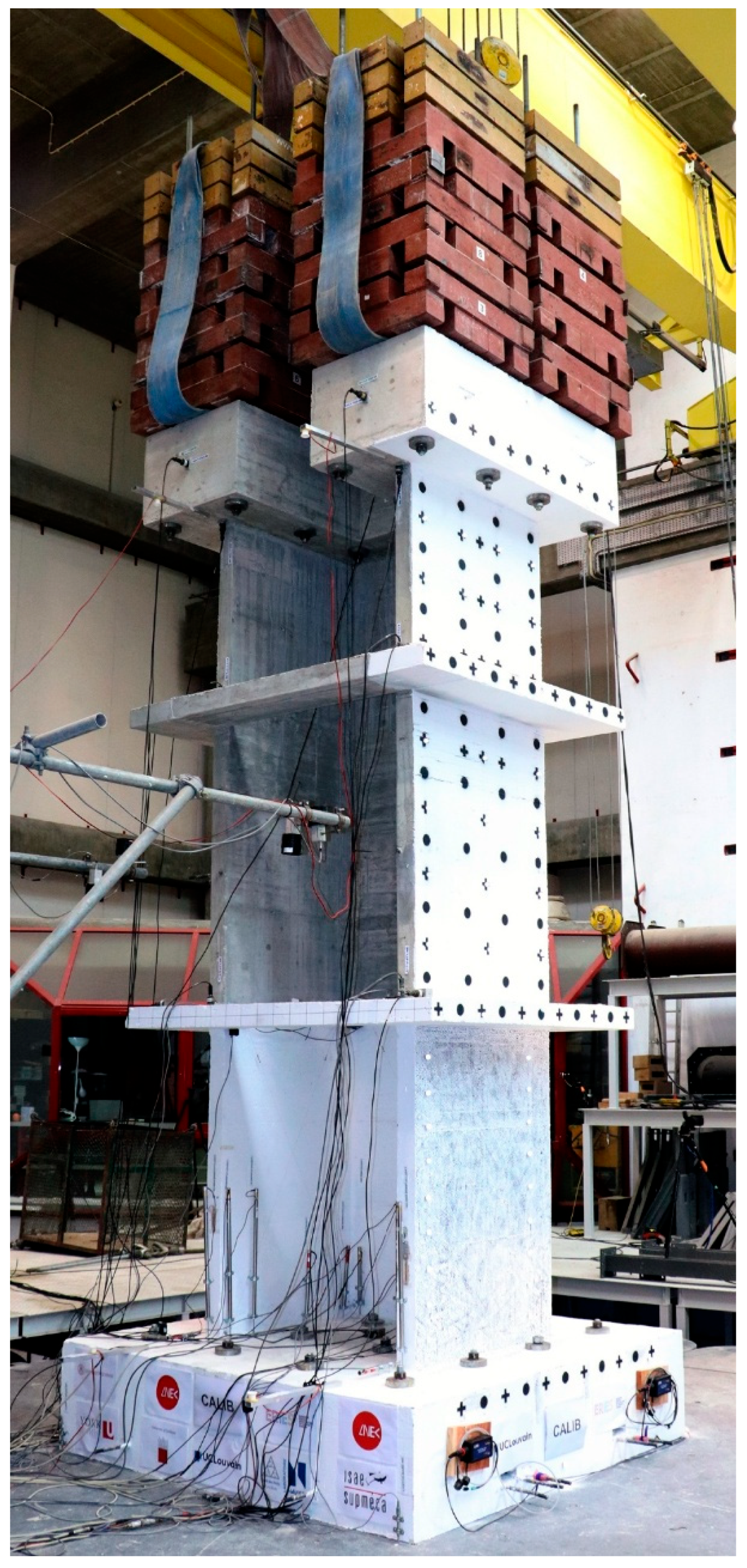
The half-scale UWS1 wall had a thickness (t_w) of 100 mm, with web and flange lengths of 1300 mm and 1050 mm (Figure 1), respectively, aligned with the section bending about its strong axis. Two hollow intermediate slabs (1.9 m × 1.62 m, 100 mm thick) were spaced 1.5 m apart (see Figure 2). The foundation block was anchored to the shake table, and to support the top masses the wall was also designed with a collar [16]. The total height from the foundation top interface to the collar center was 4.29 m. The wall was not designed to a specific code but followed capacity design principles to achieve high ductility. The boundary regions were reinforced with 12 mm diameter steel bars, while 6 mm bars were used elsewhere. Additional 8 mm bars were placed near the web-flange boundaries (see Figure 1). The boundary regions were heavily confined with 6 mm diameter hoops and stirrups at 50 mm spacing, while 6 mm shear reinforcement was spaced at 100 mm along the wall segments.

Concrete cylinder tests at 28 days indicated a mean compressive strength (f′_c) of 27 MPa. The wall was tested 41 days after casting.

Table 1. Mechanical properties of the steel reinforcing bars.

dbl	fy	fu	εsy	εsh	εsu	Es	n
[mm]	[MPa]	[MPa]	[mm/mm]	[mm/mm]	[mm/mm]	[GPa]	−
6 *	577	623	0.0028	−	0.046	208	5
6 #	550	676	0.0027	−	0.095	207	3
8	538	664	0.0027	0.0268	0.12	196	3
12	580	690	0.0029	0.021	0.101	199	3

* transverse steel (i.e., shear reinforcement, confinement ties). ^# longitudinal steel.

presents the mechanical properties of the steel reinforcement based on monotonic tensile tests.

To simulate mass effects, sixteen 1.13-ton and twelve 0.59-ton blocks were placed atop the wall collar (Figure 2), resulting in a total imposed mass of 25.16 tons. Including the 3.27-ton collar, the total mass at the top of the wall was approximately 28.43 tons.

Nine different ground motion (GM) levels were used to test UWS1, each representing a different scaling of the same west–east (WE) and north–south (NS) earthquake components. The motions were recorded from a moment magnitude 6.5 event in Italy [17] at a Joyner–Boore distance of 6.4 km. The WE component had a peak ground acceleration (PGA) of 0.81 g, while the NS component had a PGA of 0.64 g. The positive directions of the motions align with the shake table’s positive direction (see Figure 1). During testing, limited base shear sliding of the wall was observed, becoming more significant from ground motion GM7 onwards. Since incorporating sliding would require modifications to the standard modeling approaches—beyond the scope of this study—ground motions beyond GM6 were omitted. Accordingly, and also to respect space limitations, three ground motion levels are considered for a more detailed analysis: GM1, representing a uni-directional elastic response; GM5, a uni-directional nonlinear response; and GM6, a bi-directional nonlinear response. It is worth noting that nine dynamic analyses (GM0 through GM8) were performed sequentially in all numerical modeling approaches to account for damage accumulation; however, only the results for the three GMs listed in

Table 2. Scale factors (in percent) used for the ground motions.

	Scale [%]
	West–East	North–South
GM1	25	0
GM5	75	0
GM6	75	75

are evaluated in this study. The corresponding scaling factors for each GM are also listed in Table 2. The Cauchy–Froude similitude law was applied with a scaling factor of two, effectively modifying the duration of the input ground motions. The 30 s acceleration input used in the subsequent nonlinear dynamic response history analyses was recorded at 200 Hz by accelerometers mounted on top of the wall unit’s foundation.

Various instrumentation systems captured key engineering parameters during the tests. Conventional sensors included potentiometers (“string pots” or SPs) and accelerometers mounted at mid-collar height (4.29 m) and at the foundation. Linear variable differential transformers (LVDTs) measured vertical elongation inside the wall segments at the base. An OptiTrack motion capture system tracked three-dimensional displacements at selected points on the north flange and web using active markers.

4. Description of Modeling Approaches

This section provides a brief overview of the modeling approaches adopted, which span a wide range of state-of-the-practice methods.

Table 3. Summary of key features, capabilities, and limitations of the four modeling approaches.

Approach	Element Type	Features	Strengths	Weaknesses
VecTor3	3D solid elements	High modeling effort; Smeared rotating crack model; Strain penetration-explicitly represented; Limited suitability for whole-building use	Coupled flexure–shear–torsion interaction; includes strain-rate effects, dowel action, and post-yield behavior	Restricted dynamic analysis duration; No bond-slip
BTM	Beam + truss elements	Low modeling effort; Smeared (truss diagonals) model; Strain penetration-explicitly represented Suitable for whole-building use	Coupled flexure–shear–torsion interaction; flexible material modeling	Fixed diagonal angle
MVLEM-FD	Multi-fiber vertical elements	Moderate modeling effort; Implicit crack representation; Strain penetration requires additional modeling refinement; Extended version for coupled-axial-flexural-shear response; Suitable for whole-building use	Relatively simple; Physically based hysteretic nonlinearity; Adjustable cracking stiffness, Simple result processing	Estimation of some local response quantities-less reliable; Sensitive to mesh discretisation
AEM	Discrete rigid elements	Moderate modelling effort; Discrete crack representation Strain penetration-not inherently included Limited suitability for whole-building use	Hybrid FEM-DEM approach; explicit local damage and failure modeling	No equivalent viscous damping

, at the end of this section of the paper, provides a concise summary of the key features, strengths, and limitations of the four modeling approaches evaluated in this study, with further detail provided in the subsections below. While other RC wall modeling techniques exist [9,18,19,20], they are beyond the scope of this study but remain applicable for simulating core walls.

4.1. VecTor3

VecTor3 [21] (Version 2.0) is a state-of-the-art nonlinear FE analysis software for three-dimensional RC solid structures. The software incorporates the fundamental framework for analyzing the behavior of cracked RC elements under in-plane forces, namely the Modified Compression Field Theory [22] and its extension, the Disturbed Stress Field Model [23]. VecTor3 has been successfully used in previous research investigations to simulate quasi-static U-shaped wall test units [24,25,26]. Furthermore, VecTor3 has been employed to simulate the dynamic behavior of wall unit UWS1 in a separate publication [27]. As such, the same modeling approach from the previous published work is used here. A brief description of the VecTor3 numerical model of UWS1 is given below.

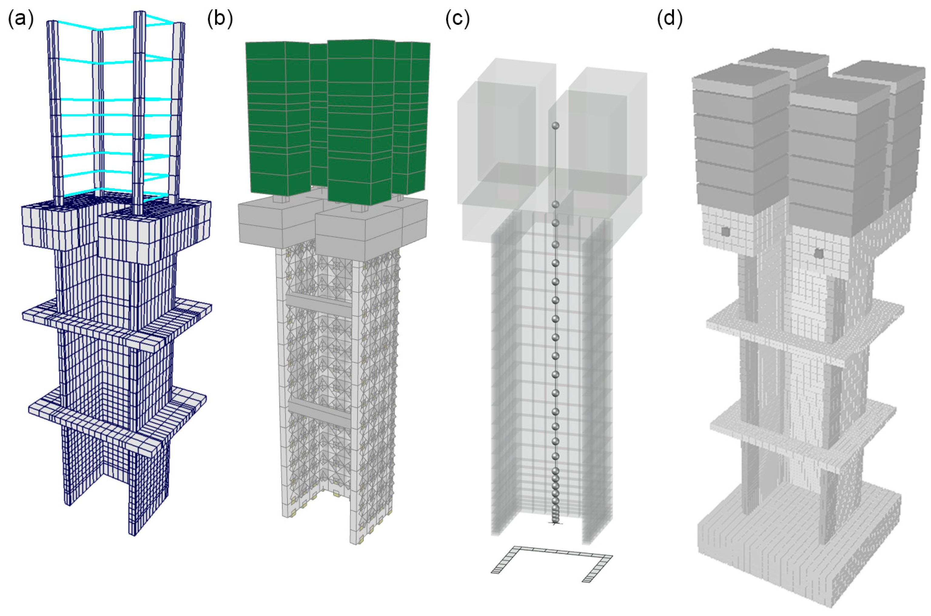
A three-dimensional wall model, shown in Figure 3a, was developed to simulate the dynamic behavior of wall unit UWS1. The model was designed to balance computational efficiency with accuracy by minimizing the number of nodes and elements while ensuring an appropriate mesh size for capturing both local and global wall responses. A prior mesh sensitivity analysis [28] guided the model development, employing eight-noded hexahedral and six-noded wedge elements for the concrete. The 12 mm rebars in the flange boundary ends were modeled using truss elements, while all other reinforcement was represented using the smeared reinforcement option. Link elements for simulating bond behavior between reinforcement and concrete are not supported in this version of VecTor3. To account for the imposed mass of 25.16 tons, rigidly elastic hexahedral elements extended the wall height above the collar to support the lumped masses.

The foundation was not explicitly modeled to reduce computational demand. However, strain penetration effects into the foundation were considered critical for accurately capturing local phenomena [27], such as base strains. To address this, a modeling approach adapted from previous studies [31,32] was used: a bottom row of FEs was incorporated below the foundation–wall interface, maintaining the same cross-section and reinforcement detailing as the elements directly above. A constant strain penetration length of 220 mm was assumed [33], based on prior distributed fiber optic sensor data from quasi-static tests of similarly detailed wall units. These foundation-level elements were assigned elastic concrete properties in compression with zero tensile capacity. The bottom nodes were fully fixed against translation and rotation, while nodes at the foundation level were only constrained against horizontal movement in both orthogonal directions.

A summary of the chosen material and constitutive models is given in the mentioned previous work [27]. VecTor3 implements an initial stiffness-based Rayleigh damping model, with a low damping value of 0.25% assigned to the first vibrational mode [27].

A key current limitation of VecTor3 is its restriction to fewer than approximately 500 data points per analysis [27]. Consequently, to respect this constraint and reduce computational time, the VecTor3 simulations used only seven seconds of acceleration input (280 data points), achieved by increasing the time step from 0.005 s to 0.025 s.

VecTor3 is particularly suitable for simulating non-rectangular, unsymmetrical, or non-planar wall geometries where two-dimensional models, such as VecTor2, may be insufficient. The former is capable of capturing complex flexure–shear–torsion interaction and dynamic effects, including strain-rate influences, dowel action, and post-yield deformation. However, some limitations remain, including the inability to explicitly model foundation flexibility, bond-slip effects, or strain penetration at the base when link elements are unavailable. Appropriate mesh refinement, element aspect ratios, and element types should therefore be selected to balance computational efficiency with simulation accuracy. When implemented with these considerations, VecTor3 provides a robust and validated framework for predicting the inelastic and dynamic behavior of RC wall systems.

For detailed implementation [34] and validation studies, the reader is referred to the literature [27,28,35,36,37,38].

4.2. Beam-Truss Models (BTMs)

The Beam-Truss Model (BTM) was developed to simulate the nonlinear flexure-shear interaction and seismic response of planar and non-planar RC walls [39,40,41]. BTMs have also been used to model RC U-shaped core walls, successfully capturing axial-flexure and axial-torsion responses under quasi-static, reverse-cyclic loading [6,32]. A brief overview of the BTM methodology is provided here.

Figure 3b illustrates the BTM of wall unit UWS1, which comprises two element types: (i) nonlinear fiber-section Euler–Bernoulli beam elements in the vertical and horizontal directions and (ii) nonlinear truss elements in the diagonal directions. The latter models the concrete’s compressive field, with its effective width determined by the element angle, calculated as 48° for this model [6]. This angle was slightly reduced to 47° for the diagonal elements in the web due to the nodal arrangement of the five vertical elements defining the web cross-section. Consistent with prior studies [6,39], the tensile strength of concrete in these diagonal elements is neglected, and no reinforcement is included in their cross-section.

The BTM was implemented in SeismoStruct [29] (Version 2026, Release 2, Built 1), a commercial software for static and dynamic analysis of framed structures. Vertical and horizontal beam elements were modeled using two-node inelastic displacement-based frame elements (infrmDB) with two Gauss–Legendre integration points. Displacement-based elements were chosen over force-based elements, aligning with common engineering software practices [9].

In SeismoStruct, infrmDB elements employ the fiber-section approach, with 150 discretized fibers assigned uniaxial stress–strain relationships. The software automatically calculates axial, flexural, and torsional rigidity for these elements. Concrete and reinforcing steel behavior were modeled using the constitutive laws of Mander, et al. [42] and Menegotto and Pinto [43], respectively.

The head of the wall was modeled using an elastic frame element (“elfrm”) with the same cross-section as the collar (see Figure 2 and Figure 3; dimensions not reported here). The elfrm was connected vertically to only two central nodes. To ensure effective force transfer across all nodes at the top of the wall in the collar, horizontal links—rigid in flexure and shear—were introduced into the model. These rigid links were assigned a torsional stiffness value of zero, based on the recommendations in Xenidis, et al. [44]. The preassigned flexural stiffness of the horizontal links significantly influenced the global response of the wall model; for example, an excessively high value led to unrealistically large wall displacements. In this study, a flexural stiffness of 0.5E_cI_link was used, where I_link was determined based on the collar cross-section. Three sets of horizontal rigid links were distributed along the height of the collar, with I_link calculated as t_collar × h_collar³/12.

Similarly, the contribution of the intermediate slabs to the global response of the wall—particularly in the north–south direction and torsional behavior—was modeled using elfrm elements on the east side of the wall. Only the slab section linking the two ends of the flanges was included. To account for cracking, a torsional stiffness of zero was assigned, and the elastic flexural stiffness values were reduced by 80%.

The same approach used in the VecTor3 model to simulate strain penetration effects into the foundation was applied to the BTM: a bottom row of vertical beam elements, each 220 mm in length, was implemented with the same restraints as before.

An initial stiffness-based Rayleigh damping model was also used to ensure comparability between VecTor3 and other modeling approaches. A damping value of 0.25% was again assigned to the first vibrational mode. However, unlike the VecTor3 model, a better match of the BTM results with the experimental measurements was achieved when a 2% damping value was assigned for the post-yield analyses (i.e., for GM5 and GM6), which was therefore adopted for these runs.

BTMs are particularly well suited for walls in which nonlinear shear deformation, torsion, and warping effects play an important role, including non-planar wall systems, where conventional wide-column or stick models may be inadequate. Care should be taken in defining boundary conditions, including base fixity and potential rotational flexibility, as these can significantly influence global response. While simplified assumptions are commonly adopted for concrete tension and reinforcement buckling in diagonal elements, appropriate strain limits and material models should be employed to enable meaningful interpretation of damage and performance states. When implemented with adequate discretisation and informed parameter selection, BTMs provide a robust and computationally efficient framework for simulating the inelastic seismic response of both planar and non-planar RC wall systems.

For detailed formulation, implementation strategies, and validation studies, the reader is referred to the original BTM developments [39] and subsequent extensions [40,45], addressing shear–flexure interaction and seismic wall response.

4.3. Multiple-Vertical-Line-Element-Model (MVLEM-FD)

The response of UW1 was analyzed using a three-dimensional (3D) version of the force-displacement-based multiple-vertical-line element (MVLEM-FD) developed at the University of Ljubljana [46]. The wall cross-section was subdivided into smaller segments (see Figure 3c), based on the distribution, positioning, and amount of longitudinal reinforcement. Each segment was represented by a corresponding vertical spring. These springs are rigidly connected at each node, simulating coupled axial–flexural behavior under Bernoulli’s hypothesis (“plane sections remain plane”). The wall was also subdivided vertically into smaller elements, with shorter elements placed in the potential plastic hinge region. The positions and number of vertical springs were kept the same along the entire height of the wall.

The boundary elements of the wall were considerably reinforced (see Figure 1). Drawing insights from prior studies [47], the corresponding segments were modeled using a dual-material approach by modeling the concrete (VertSpringType2) and reinforcement (ReinforcingSteel) separately, using two different material models connected in parallel. The buckling model by Dhakal and Maekawa [48] was considered when modelling the boundary elements of the wall to account for potential buckling of the longitudinal reinforcement. The inner segments between boundary elements were modelled using single VertSpringType2 material, combining the contributions of both reinforcement and concrete. The hysteretic response of the vertical springs was defined using standard parameters proposed by the authors [46].

In the basic version of the MVLEM-FD, shear and torsional response are simulated using the shear and torsional springs located at the centroid of the cross-section (in the horizontal plane) and the center of rotation of the corresponding element (in the vertical plane), respectively. In the MVLEM-FD, shear and torsional responses are uncoupled from flexural response. Extended formulations of the element [47], however, can couple axial, flexural, and shear behaviors [49].

As previously mentioned, shear sliding of the wall was observed. Therefore, in the lower shear springs, the shear response was modeled as inelastic. To describe the force-displacement hysteretic response of these springs, two shear mechanisms that transfer shear force over the cracks were considered: the dowel effect of vertical bars [50], and interlock of aggregate particles in the crack [51]. Their parameters were calibrated using results from optical measurements [11]. In OpenSees, their response was described using a hysteretic uniaxial material.

Longitudinal reinforcement serves two primary functions: to provide flexural resistance and to prevent shear sliding via the dowel mechanism. Based on experimental observations, the longitudinal bars in the web were assumed to primarily transfer shear forces. Hence, in the vertical springs corresponding to these segments, flexure resistance was not considered. Conversely, the longitudinal reinforcement in the boundary elements was assumed to contribute solely to flexural resistance, with no contribution to shear strength.

The elastic deformation of the prestressing rods fixing the foundation to the shake table resulted in base rotations. The latter were limited and capped by the bending moment capacity of the wall. Nonetheless, they contributed proportionally more to the total deformation during the lower excitation intensities (GM0–GM2). Consequently, they were simulated using rotational springs at the bottom of the wall. When defining the properties of these springs—which are considered uncoupled in the two perpendicular directions—the results of LVDTs were taken into account. They were modeled using an elastic uniaxial material.

Considering experiences in modeling different shake table tests [52,53,54] and the relatively low level of axial forces involved, the initial stiffness was reduced three-fold compared to that corresponding to the gross cross-sectional properties.

A 2% viscous damping was considered for the two first modes, and implemented using the Rayleigh damping model. Following recommendations from the literature [55,56], the damping matrix was defined considering the structure’s mass and initial stiffness.

When modeling RC walls with the MVLEM-FD, accurate discretization both along the height and across the cross-section is essential; in particular, the mesh should be refined in the potential plastic-hinge region and the cross-section subdivided to represent the actual reinforcement layout. For boundary elements with substantial reinforcement, adopting a dual-material representation (separate concrete and reinforcement components, including a buckling model for longitudinal bars) improves the accuracy of the flexural response. This formulation should be used when its influence on the overall behavior is expected to be significant.

If the wall response is governed primarily by flexure, the basic MVLEM-FD formulation is appropriate. However, when shear–flexure interaction significantly influences the response, the extended MVLEM-SFI formulation, which couples axial, flexural, and shear response, should be employed. Modeling boundary conditions—for instance, base rotations—is essential and should be considered whenever such effects may influence the structural response. Appropriate damping parameters should likewise be selected to ensure accurate dynamic behavior.

For detailed modeling guidelines, the reader is referred to the basic MVLEM-FD formulation [46], the extended MVLEM-SFI formulation [49], and related recommendations for modelling RC walls under dynamic loading [47,52,54].

4.4. Applied Element Method (AEM)

The Applied Element Method (AEM) [57], combining the strength of the continuous FE formulation with the advantages of discrete models, has in the recent years been increasingly employed to assess the failure mechanisms developed by structures subjected to dynamic loading. However, the AEM, of which a detailed description is provided in Orgnoni [58], has been seldomly used in the literature to simulate the local and global quasi-static response of RC walls. Recently, this framework was applied successfully to the numerical modeling of the out-of-plane behavior of thin RC walls [58], as well as for the accurate quasi-static, reverse cyclic simulation of two RC core walls subjected to flexural and torsional loading protocols [59]. Furthermore, the AEM has been employed to simulate the dynamic behavior of wall unit UWS1 in a separate publication [60]. As such, the same modelling approach from the previous published work is used here. For sake of brevity, a short description of the AEM numerical model of UWS1 is given below.

The numerical model of specimen UWS1 was implemented in the computer program Extreme Loading for Structures (ELS) [30]. The approach adopted for the definition of the structural mesh, represented in Figure 3d, is described in Orgnoni, et al. [60] and followed that outlined by Orgnoni and Pinho [59], herein briefly summarized. The foundation and the collar were modeled adopting a coarse mesh with dimensions equal to ~100 mm per element. Regarding the web and flanges, a reasonable departure hypothesis is that the deformations will be concentrated between the foundation and the first slab, while the upper region will mainly behave in an elastic manner. Therefore, a fine mesh equal to 0.5t_w (50 mm) was used below the first slab and for the intermediate slabs, whilst a coarser mesh of 1.0t_w was employed in the remaining upper portion of the wall. The top masses were implemented explicitly through the introduction of elements, rigidly connected to the collar, that have the same dimensions and density of the mass blocks employed in the test. Overall, the numerical model features 10,854 elements, each of which with twenty-five springs (5 × 5) implemented at the contact faces with neighboring elements. Three different types of concrete materials (namely, confined, partially confined, and unconfined) were implemented using the Mander, et al. [42] constitutive model, to account for the confinement effect provided by the reinforcement layout. The rebars are implemented by means of a single spring (for each bar) at the elements’ interfaces; for this reason, rebars are assumed to be fully bonded with the concrete. Foundations and collar were characterized by an elastic material featuring the uncracked stiffness of the concrete. The 30 s long accelerograms recorded atop the foundation fixed to the shake table during the test were used as input for the model, with a time-step of 0.005 s (200 Hz). No external damping contribution was applied to the numerical model.

5. Comparison of Numerical and Experimental Results

The following sections summarize the global and local response estimates of wall unit UWS1 based on the four modeling approaches considered in this study. Each section specifies the instrument used to measure the experimental response, ensuring that researchers and engineers can reproduce the experimental plots using the dataset available in the open repository [61]. For consistency, and whenever possible, the same methodology was applied to derive numerical estimates.

5.1. Displacement, Rotation, and Acceleration History Response

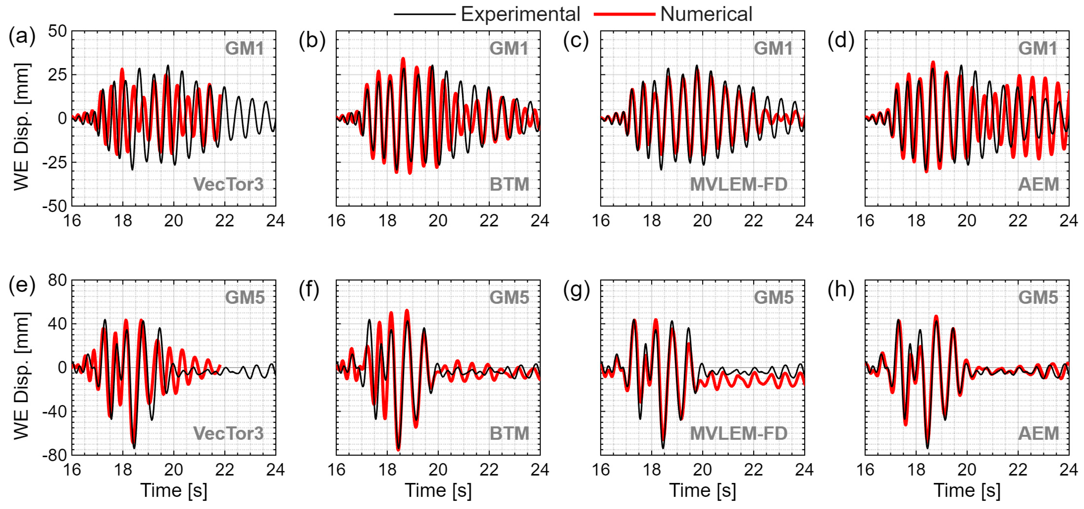
Figure 4a–d presents the west–east displacement (“WE disp.”) response histories for the four modeling approaches used in this study under GM1. The experimental measurements were obtained by averaging the readings from two potentiometers (SP10 and SP11) positioned 4.29 m above the foundation on the eastern face of the collar (head) to the north and south, then subtracting the displacement of the shake table (PosA1T). A small foundation uplift, ranging from 0.5 to 1.0 mm, was observed experimentally during the initial stages of the ground motions. Assuming rigid body motion, this uplift could account for approximately 4–8% of the measured top displacement of the wall under GM1. All models reasonably capture the peak displacements during the cracked-elastic stage of wall behavior, with the MVLEM-FD and BTM approaches seemingly providing the closest match to experimental measurements. As discussed elsewhere [27], selecting a small damping ratio—between 0.25% and 1%—was crucial for obtaining the most accurate predictions in nonlinear dynamic response history analyses from VecTor3 and BTM. This is particularly important for lower-intensity ground motions, where the structure remains in the pre-yield stage, and energy dissipation is not primarily governed by the implemented models of material hysteresis. It is noted that the AEM model applies no equivalent viscous damping; whilst this has negligible impact at higher ground motion intensities where hysteretic energy dissipation is dominant, it manifests in the inability of the AEM to adequately reproduce the experimentally observed displacement amplitude decay in the later stages of GM1 (after approximately 22 s, Figure 4d), where the specimen remains largely in the pre-yield stage and material hysteresis is limited.

Figure 4e–h presents the WE disp. response histories for the wall’s post-yield behavior under GM5. All four modeling approaches predict peak displacements within 10% error, demonstrating their applicability in simulating the wall’s global response to a flexure-governed response from unidirectional ground motions about its weak (minor) axis. While VecTor3 provides reasonable estimates, the BTM, AEM, and MVLEM-FD approaches more closely capture the full displacement history under GM5. However, MVLEM-FD predicts larger residual displacements at rest than those observed experimentally. This discrepancy may be attributed to the exclusion of explicit or implicit modeling of strain penetration into the foundation, which would lead to larger tensile strains at the wall base compared to the experimental response. This issue is investigated further later in the paper, see Section 5.4. The larger plastic tensile strains predicted by MVLEM-FD are therefore also likely responsible for the residual deformations observed in the numerical results.

For higher-intensity ground motions inducing post-yield inelastic behavior (e.g., GM5), the assigned damping values became less critical, as energy dissipation was primarily governed by material hysteresis.

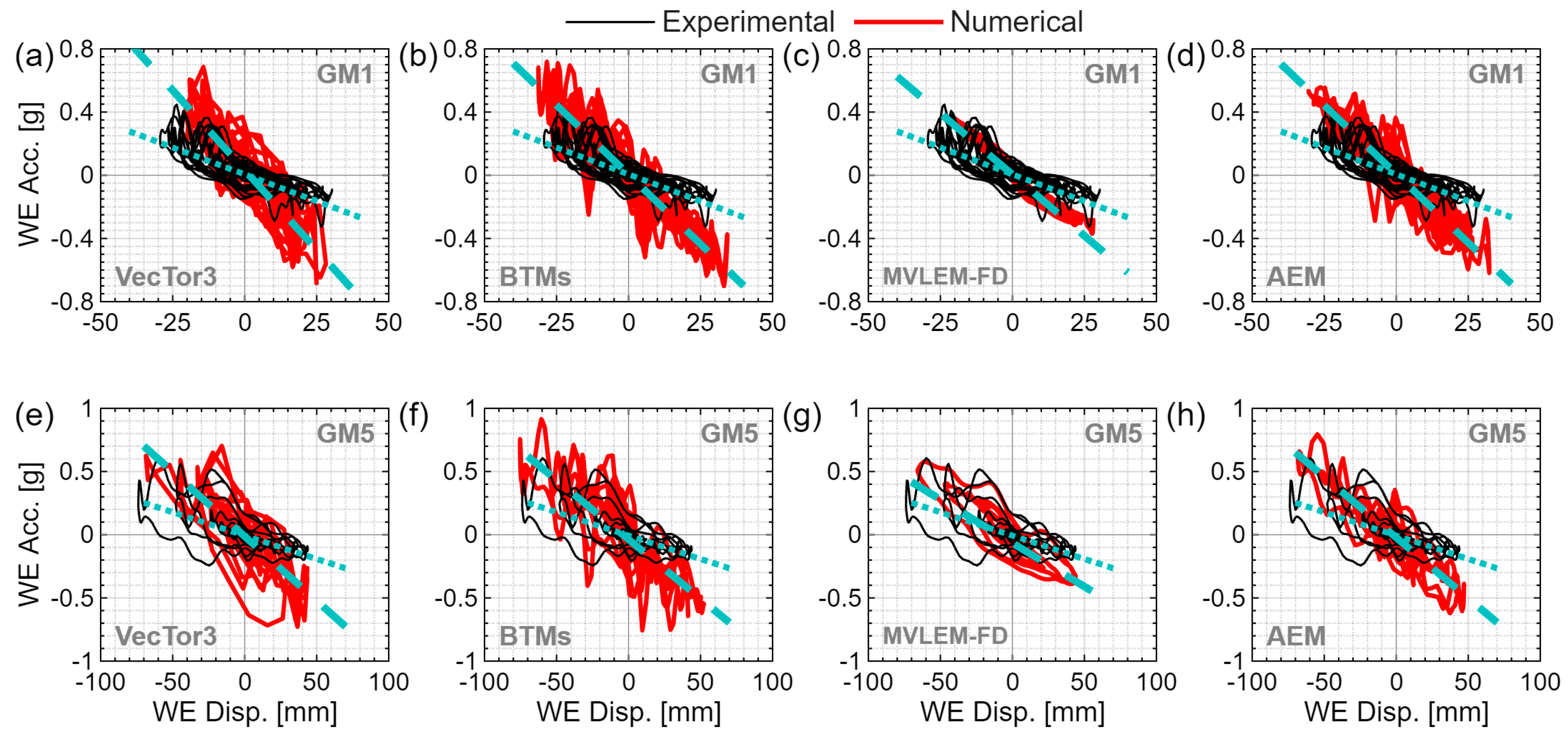
Figure 5 presents west–east acceleration (“WE Acc.”)–displacement hysteresis plots for the unidirectional ground motions of GM1 (a–d) and GM5 (e–h) using the four modeling approaches. The experimental absolute acceleration was measured using an accelerometer (A01) positioned at the center of the eastern face of the collar (head), 4.29 m above the foundation. Since acceleration is proportional to force, the average slope as a proxy for stiffness is included in these plots to further assess the models’ ability to capture the force-displacement response. The average stiffness is determined using a linear regression analysis (i.e., a linear trendline), which represents the secant stiffness connecting the maximum and minimum accelerations. This approach is similar to that used by Hoult and Beyer [25] for torque-rotation. The cyan-dotted line represents the average stiffness derived from the experimental dataset, while the cyan-dashed line corresponds to the average stiffness obtained from the numerical analyses.

All modeling approaches overestimate the wall’s stiffness for both unidirectional ground motions GM1 and GM5. It should be noted that the average slope of the acceleration–displacement relationship is used here as a proxy for stiffness rather than a direct measure of it, and should be interpreted with appropriate caution. In particular, the experimental acceleration–displacement response (in the west–east direction, Figure 5) shows notable asymmetry between the positive and negative loading directions, particularly under GM5 (Figure 5e–h), meaning that an averaged slope over both directions may introduce additional discrepancy relative to the numerical results. Interestingly, despite the apparent differences in slope between the numerical and experimental acceleration–displacement relationships, the displacement response histories (in Figure 4) show generally good agreement in terms of vibration period during the higher-amplitude phases of the response. This suggests that the effective dynamic stiffness may be better captured than the acceleration–displacement plots alone imply. The source of this apparent inconsistency is not fully resolved and may warrant further investigation, including consideration of how local effects influenced the recorded accelerations.

Under GM1 (Figure 5a–d), only the MVLEM-FD model underestimates the peak acceleration, while the others exceed it by more than approximately 40–60%. In contrast, the models better capture the acceleration–displacement response for the inelastic behavior under GM5 (Figure 5e–h), albeit still overestimating the peak acceleration within the range of 20–50% for most models. The exception to this is the MVLEM-FD approach, which underestimated peak acceleration by approximately 4%.

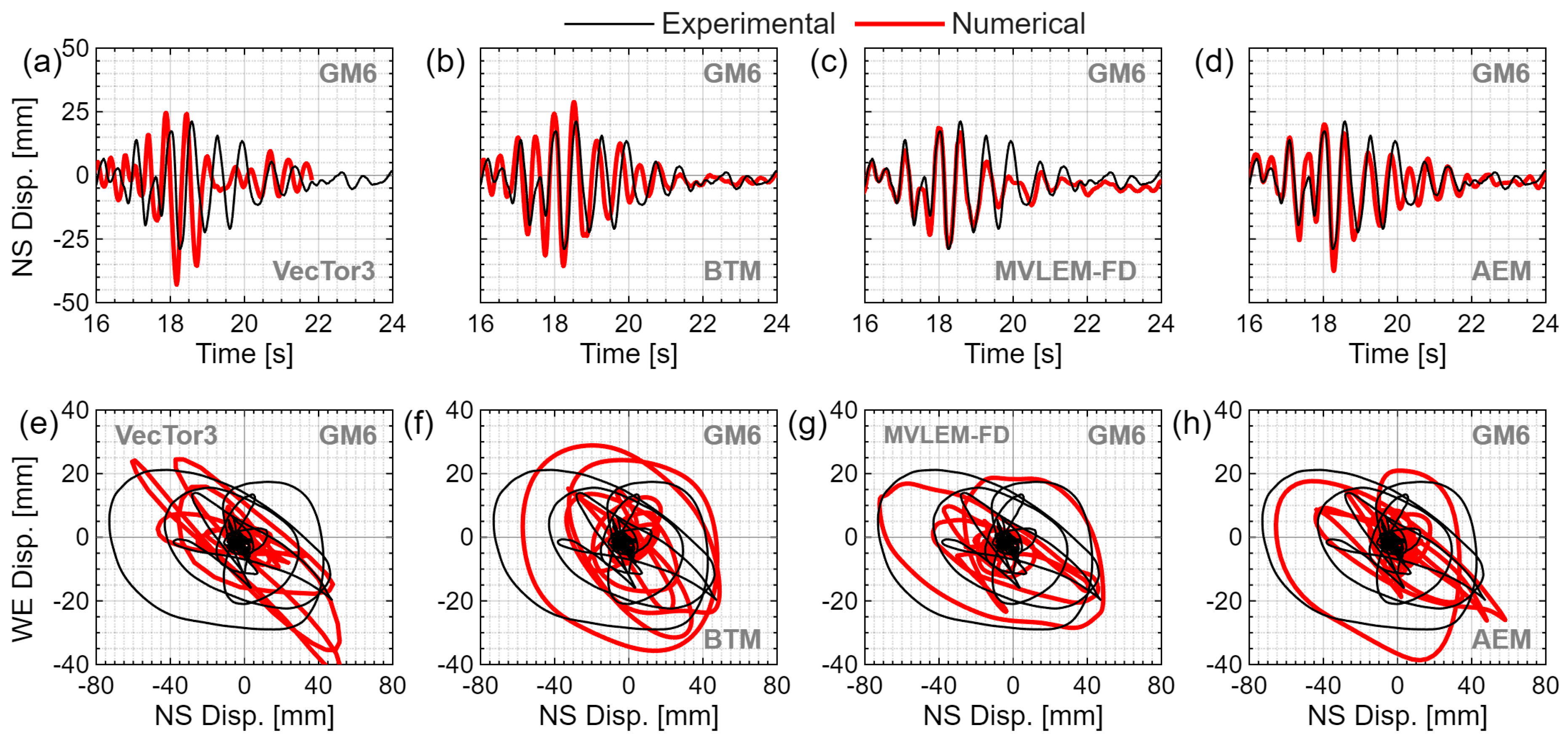
Modeling the wall’s response in the north–south direction proved more challenging due to the complexities of bidirectional GM6, which also induced rotation about the vertical axis. Figure 6a–d presents the north–south displacement (“NS disp.”)-response histories for the four modeling approaches under GM6. The experimental measurements were obtained by averaging the readings from two potentiometers (SP07 and SP08) along the north–south direction, positioned 4.29 m above the foundation on the northern face of the collar (head) to the east and west, then subtracting the displacement of the shake table (PosA2L). Overall, the simulations provide reasonable estimates of peak displacements. For VecTor3, modeling the slab and collar (head) as elastic and rigid was essential for obtaining a more realistic response—yet the peak displacement was estimated to be almost 50% greater than the measured values even with these considerations. The BTM also overpredicted the peak displacements but with a smaller error of approximately 24%, and showed improved agreement with the displacement–response history. It is important to note that the bidirectional response in the BTM was highly sensitive to the assumed properties of the rigid links used in the collar (head) of the wall model—see Section 4 for further details. The MVLEM-FD approach yielded the closest match to the peak absolute displacement, with an error of approximately 2%.

To better illustrate the wall’s bidirectional response, Figure 6e–h plot the WE displacement as a function of NS displacement under GM6. The bidirectional response from VecTor3 is suboptimal, as shown in Figure 6a. In contrast, the BTM, MVLEM-FD, and AEM approaches demonstrated more realistic bidirectional behavior, as evident from the traces in Figure 6f–h.

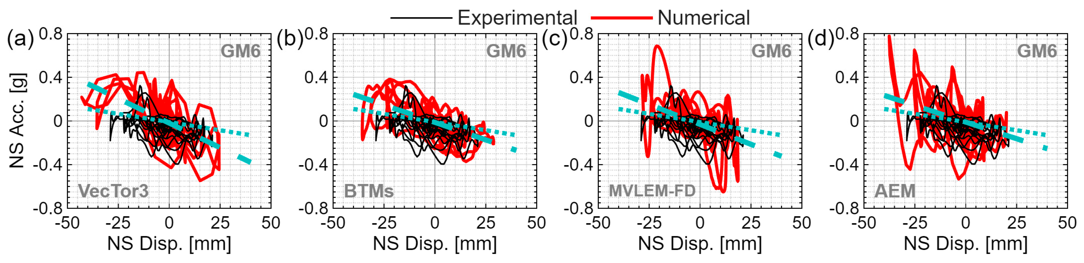
Figure 7 presents the north–south absolute acceleration (“NS Acc.”)–displacement hysteresis under bidirectional GM6 for the four modeling approaches. The experimental absolute acceleration was measured using an accelerometer (A07) positioned to the west of the southern face of the collar (head) at 4.29 m above the foundation. Unlike the east–west direction (Figure 5), where stiffness was generally widely overestimated, most models provided a closer match to the experimentally derived average stiffness. Although the MVLEM-FD reproduced the overall NS acceleration trace under GM6 with reasonable accuracy (Figure 6c), it overestimated some peak accelerations (Figure 7c). It is worth noting, however, that these numerical acceleration peaks coincide with isolated time steps where non-convergence occurred. The other models also overpredict peak absolute north–south accelerations, particularly the AEM, with the BTM providing the closest fit.

5.2. Torque-Rotation

As noted earlier, modeling the wall’s north–south response was more challenging due to its coupled torsional behavior. This torsion arises primarily from the shear center being located outside the section [25,62] and the slight offset (by approximately 24 mm) of the imposed mass blocks from the wall’s geometric centroid [13,15]. All modeling approaches relied on certain assumptions regarding the wall’s overall rotational response, particularly in representing the intermediate slabs, collar (head), and mass blocks.

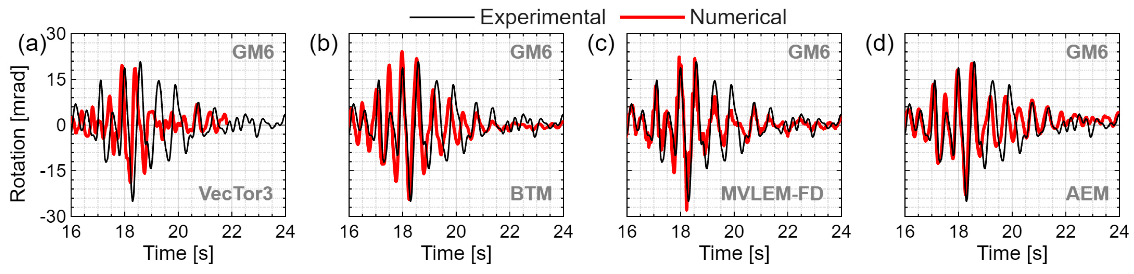
Figure 8 presents the wall’s rotation response histories under GM6 for the four modeling approaches. The experimental measurements were obtained by subtracting the readings from two potentiometers (SP10 and SP11), positioned 4.29 m above the foundation on the eastern face of the collar (head) to the north and south, and dividing by the 1.2 m lever arm distance between them. The displacement of the shake table (PosA1T) was also subtracted. In general, the models provide reasonable estimates: VecTor3 underestimates the peak rotation by approximately 20%, the MVLEM and AEM predict values within an 8–12% margin of error, and the BTM approach achieves the closest match, with deviations limited to about 2%.

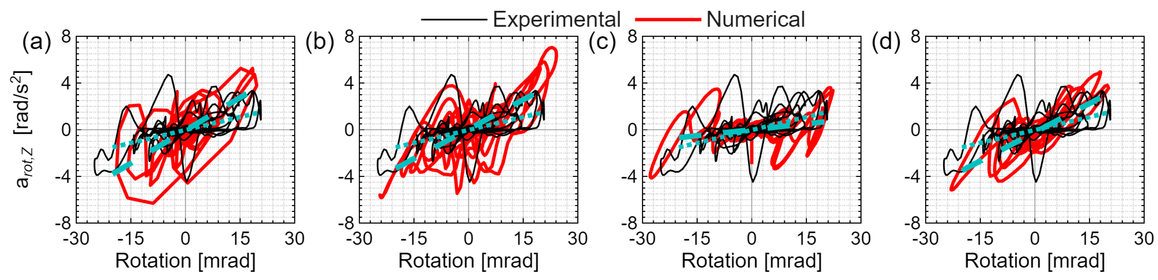
The angular acceleration about the vertical axis (a_rot,z) at the top of the wall was estimated experimentally and numerically using Equation (1) (all symbols are defined in the Notation section). In principle, the corresponding torque could be obtained by multiplying a_rot,z by the rotational inertia of the top mass. However, accurately doing so requires knowledge of the shear-center location, which is difficult to quantify as it has been shown to shift toward the web as a function of imposed drift [25]. For this reason, comparisons in this study are made directly to a_rot,z.

$$a_{rot,z}=\left({\displaystyle \frac{1}{L_x}}\right)\left(a_4-a_2\right),$$

(1)

The angular acceleration–rotation hysteresis plots for the four modeling approaches are given in Figure 9. Most modeling approaches predict a stiffer wall response compared to the experimental data. The exception is the MVLEM-FD approach in Figure 9c. Vector3 and BTM overestimate the absolute peak a_rot,z, while the MVLEM-FD and AEM remain within a 9–12% margin of error.

5.3. Base Strain Profiles

In this section and the next, strain profiles are examined at selected timestamps. However, in cases where the numerical and experimental global displacement response histories differ at these timestamps, strain profiles were extracted from the numerical model at a displacement level comparable to the experimental measurement. This ensures a meaningful comparison between numerical and experimental results.

This section examines base strains across the cross-section. Previous quasi-static tests have investigated this [1,63,64], concluding that the Bernoulli–Euler hypothesis—that plane sections remain plane—is a reasonable assumption for deriving strain gradients. However, this assumption breaks down when torsion is introduced in U-shaped sections due to warping. Limited experimental data from specimens subjected to quasi-static reverse twisting about the wall’s vertical axis indicate that a linear strain profile across each wall segment (i.e., web and flanges) remains a reasonable approximation of the strain distribution [63,64] under torsion. To the authors’ knowledge, this is the first study to investigate these local demands (strain profiles) using data from dynamic shake table tests for RC walls.

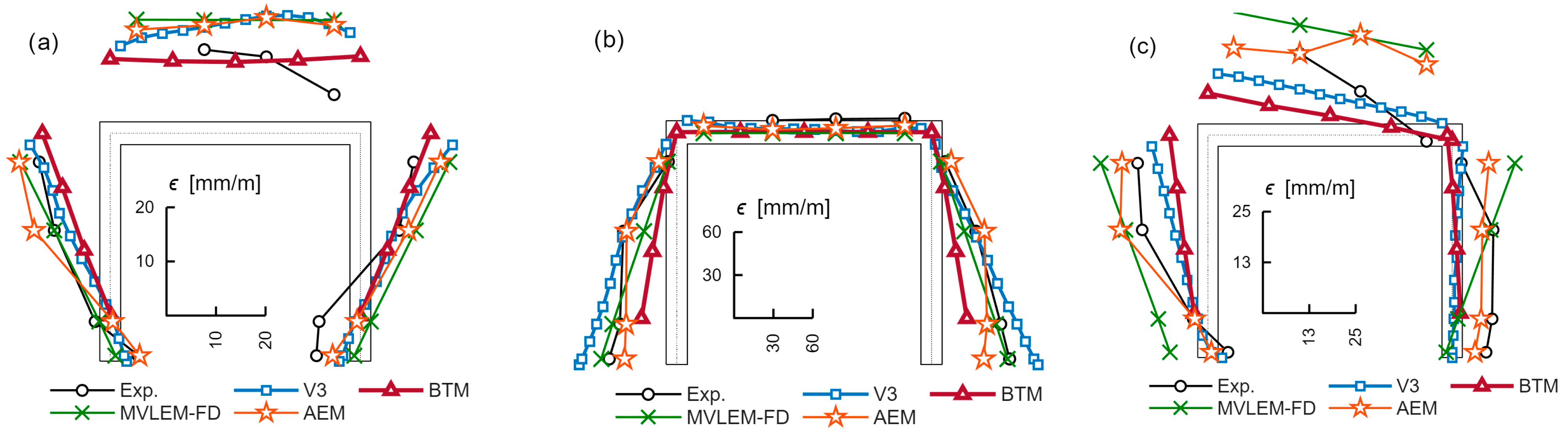
Figure 10 illustrates the base strains of the wall corresponding to the largest displacements to (a) the east and (b) the west, during GM5, and (c) rotation during GM6. The base strains were determined experimentally using an array of LVDTs positioned at the base of the wall, attached to the U-shape inside surface over a 70 mm base length. All models provide reasonably accurate base strain responses at all timestamps and for the two GMs, with the MVLEM-FD offering better tensile strain estimates near the boundary ends for westward displacement (Figure 10b). For eastward displacement (Figure 10a), tensile strains in the web are generally overestimated, although the BTM performs relatively well. This overprediction can be partly explained by the fact that the LVDTs were mounted on the inner surface of the wall, while some of the numerical strain outputs were derived from within the section, depending on the modeling approach. Assuming plane sections remain plane, simple calculations based on the offset between the numerical extraction point and the LVDT location suggest this could account for a 5–10% reduction in the predicted tensile web strains. The models struggle to capture base strains accurately when the wall undergoes rotation (Figure 10c). This is particularly true for those based on the Euler–Bernoulli assumption (e.g., MVLEM-FD), where the plane sections assumption fails under warping. For other models, such as VecTor3, poor simulation of north–south motion combined with torsional effects may contribute to the observed discrepancies.

5.4. Longitudinal (Vertical) Strain Profiles

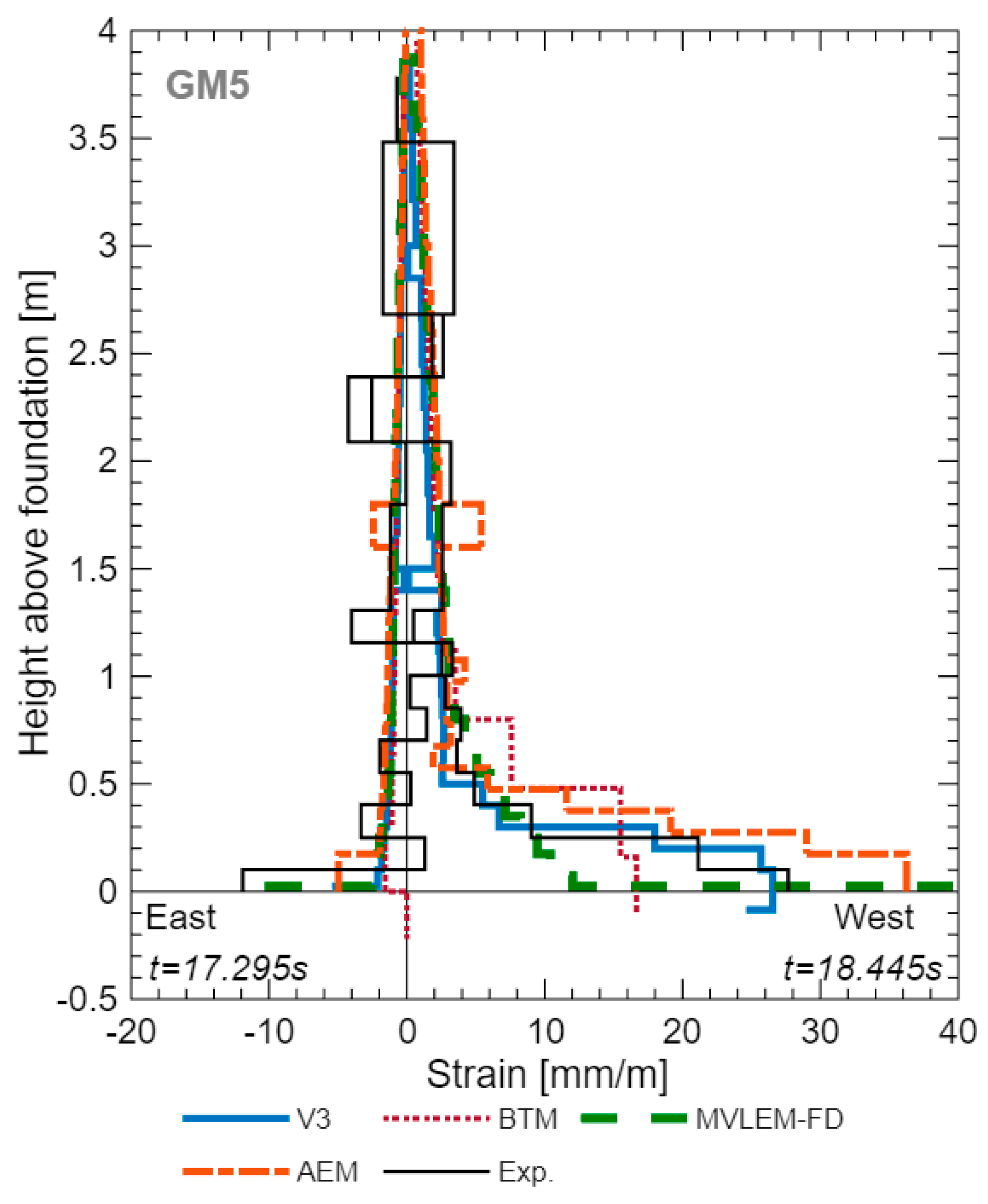
The OptiTrack motion capture system was employed to assess the longitudinal strain profiles along the height of the north flange boundary end (see Figure 1) under post-yield behavior during GM5. Tracking markers were attached to the outer surface of the north flange, positioned approximately 75 mm from the boundary edge and spaced vertically at ~150 mm, with minor deviations introduced by the presence of intermediate slabs.

Figure 11 presents the strain profiles of the north flange boundary end at two time instants, corresponding to the peak in-plane eastward (compression) and westward (tension) displacements recorded during GM5. The numerical strain comparisons were derived from the vertical deformations of nodes near the north flange boundary end. All numerically derived strain profiles show reasonable agreement in compression but generally fail to capture the large compression strains observed at the base. This aligns with previous findings for VecTor3 [27], which has been shown to be incapable of simulating concrete crushing at the wall base and does not account for strength degradation, contrary to experimental observations. With the exception of the MVLEM-FD, which shows a much closer match to the experimental results, the BTM and AEM significantly underestimates the base compression strain compared to experimental measurements.

The numerically determined tensile strains from VecTor3 under GM5 closely match the experimentally measured profile. The tensile strain profile from the AEM appears to have accurately predicted the yielding (or plastic) height at the base but overestimates the tensile strains in this region over a height of approximately 600 mm. The tensile strain profiles from the BTM and MVLEM-FD were also reasonable, though the latter significantly overestimated the tensile strains at the base (7.1% numerically compared with the experimental value of 2.8%). Accurately simulating tensile base strains in RC walls is challenging without explicitly accounting for strain penetration into the foundation—a mechanism included in the BTM and VecTor3 models but not in the present implementations of MVLEM-FD and AEM. It is noted that strain penetration can be incorporated into the MVLEM-FD formulation if required; its omission here reflects a modeling choice rather than a model limitation. Users should nonetheless exercise caution when applying modelling approaches that do not account for strain penetration for strain-based performance assessment or local ductility demand estimation.

5.5. Shear Deformations

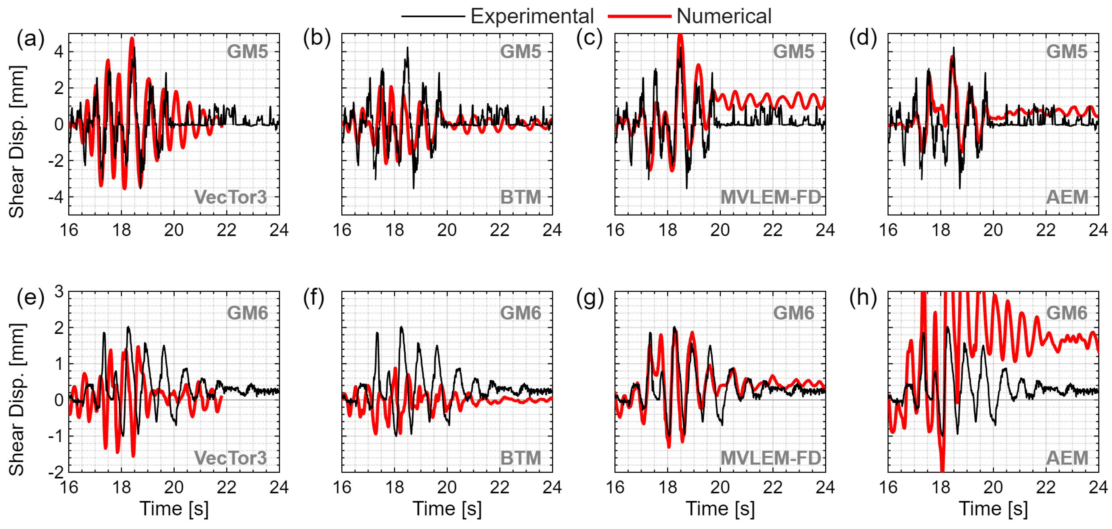
Shear displacements (Δ_s) were calculated using the standard expression in Equation (2). As highlighted by Hiraishi [65], the “α” term in Equation (2) becomes important for RC walls where curvature along the height of the wall panel is not constant. OptiTrack motion capture data, obtained from markers placed in vertical arrays along the eastern and western edges of the north flange, were used to calculate Δ_s of the north flange over the first-story height (1.45 m) under GM5. From these measurements, relative flange rotations (with respect to the markers attached to the foundation below the wall) were derived, allowing the calculation of “α” values at each time step using Equation (3) and, in turn, a corrected Δ_s time history using Equation (2). This correction, which subtracts the contributions of flexural rotation and sliding, was considered especially important under the unidirectional loading of GM5, where large flexural demands on the wall flanges were expected.

For the web shear deformations, the motion-capture data appeared noisy, likely due to (i) the very small shear displacements (<2 mm), which reduced measurement precision, and (ii) the cameras capturing the web’s outer surface being mounted on a platform separate from the other cameras (used to record the north-flange surface; see Figure 1). This platform may have vibrated during shake-table operation, degrading the measurement quality from those cameras. As such, a pair of diagonal potentiometers (SP01 and SP02) were used to directly measure shear deformations on the inside surface of the web over the first-story height. For these calculations, Equation (2) was again applied, with the “α” term assumed to be 0.5, based on comparison with motion capture data under GM6, which suggested this provided a reasonable estimate of Δ_s in the web from the potentiometer measurements.

$${∆}_s={\displaystyle \frac{1}{4b}}\left({\left(d+{\delta }_2\right)}^2-{\left(d+{\delta }_1\right)}^2\right)-(\alpha -0.5)\theta (h_{sh})h_{sh},$$

(2)

$$\alpha ={\displaystyle \frac{{\int }_0^{h_{sh}}\theta \left(z\right)dz}{\theta \left(h_{sh}\right)h_{sh}}},$$

(3)

Figure 12a–d shows the experimental and numerical Δ_s over time for the north flange under GM5. Both VecTor3 and MVLEM-FD capture the shear displacement response reasonably well, including the positive peak, with errors of 12% and 19%, respectively. The MVLEM-FD model predicts some residual displacements after 20 s, which are not observed in the experimental data. It should be noted that the standard MVLEM-FD formulation was used here, and extended versions may provide more accurate shear predictions [47]. The AEM approach also reproduces the shear displacements of the north flange under GM5 reasonably, with the corrected shears underestimating the peak by just 12%. BTM also underpredicts the peak, capturing only about 50% of the experimental maximum. This underprediction likely reflects a combination of factors inherent to the BTM formulation: the fixed diagonal element angle (48°), which governs the orientation and effective width of the concrete compressive field and may not optimally capture the shear transfer mechanism under unidirectional flexural loading; and the use of displacement-based beam elements, which are inherently stiffer than force-based formulations that satisfy equilibrium exactly, and may therefore underestimate shear deformations. The authors note that these are inherent characteristics of the BTM as implemented here rather than user-controlled parameters, and that extensions to the BTM formulation addressing shear-flexure interaction (referenced in Section 4.2) may offer improved shear predictions for future studies.

Figure 12e–h presents the Δ_s response histories of the web under GM6. Overall, the numerical models struggle to capture these relatively small shear displacements. An exception is the MVLEM-FD approach (Figure 12g), which predicts peak shear displacements within a 7% margin of error. It should be noted that the shear-spring parameters in the MVLEM-FD were calibrated against optical measurements to capture shear slip at the wall–foundation interface; the web shear displacements plotted in Figure 12e–h, however, represent deformation above the interface level, with the interface slip contribution handled separately and consistently in both the experimental processing and numerical extraction. The calibration was therefore not performed directly against the plotted response quantity, though readers should remain aware of this relationship when interpreting the close agreement achieved by the MVLEM-FD for web shear displacements. VecTor3 (Figure 12e) and BTM (Figure 12f) provide the next closest estimates, though they still underpredict peak values by 30–60%. The AEM results exhibit residual displacements that are not observed in the experimental data.

6. Implications for Engineering Design Practices

As stated in the introduction, accurately designing RC buildings, particularly in seismic regions, requires a thorough understanding of their nonlinear dynamic behavior under earthquake loading. Nonlinear response-history analysis (NLRHA) has become a crucial tool for assessing the complex response of these structures, capturing key phenomena such as stiffness degradation, strength deterioration, and energy dissipation. Compared to nonlinear static analyses (e.g., pushover), NLRHA is generally considered to provide a more realistic representation of inelastic deformations and failure mechanisms in RC structures.

However, as demonstrated in this work, structural demand variability from earthquake ground motions arises both from aleatory variability and epistemic uncertainty—such as assumed material parameters, modeling constraints, and the mathematical representations of both materials and structural behavior. Therefore, sophisticated models must first be validated against physical tests, such as those explored in this study.

In the analysis and design of RC structures using NLRHA, specific demand parameters are typically selected to quantitatively evaluate performance levels, often including peak deformations. This section summarizes the results presented earlier by comparing key demand parameters obtained from the different numerical approaches to experimentally measured values.

Table 4. Summary of engineering parameter values extracted from the four modeling approaches. ‘Exp.’ denotes experimental (values), ‘Comp.’ represents compression, and ‘BE’ refers to the boundary end. The relative error values are shaded to highlight particularly poor estimates from the numerical models, with blue indicating underprediction and red indicating overprediction. The shading intensity reflects the magnitude of the error, with brighter colors corresponding to greater inaccuracy.

		Exp.	VecTor3		BTM		MVLEM-FD		AEM
		-	-	Rel. Error	-	Rel. Error	-	Rel. Error	-	Rel. Error
Global Demand Parameters	Maximum absolute EW drift (%), GM1	0.71	0.66	−7%	0.80	13%	0.65	−8%	0.75	6%
	Maximum absolute EW drift (%), GM5	1.72	1.60	−7%	1.76	2%	1.53	−11%	1.59	−8%
	Maximum absolute EW drift (%), GM6	1.70	1.41	−17%	1.33	−22%	1.68	−1%	1.46	−14%
	Maximum absolute NS drift (%), GM6	0.67	1.00	49%	0.83	24%	0.66	−1%	0.88	31%
	Maximum absolute rotation (mrad), GM6	25.0	19.6	−22%	24.4	−2%	27.9	12%	23.0	−8%
	Maximum absolute EW acceleration (g), GM1	0.45	0.69	53%	0.72	60%	0.37	−18%	0.62	38%
	Maximum absolute EW acceleration (g), GM5	0.61	0.73	20%	0.91	49%	0.58	−5%	0.80	31%
	Maximum absolute NS acceleration (g), GM6	0.40	0.55	38%	0.38	−5%	0.69	73%	0.78	95%
	Maximum absolute angular acceleration (rad/s2), GM6	4.73	6.31	33%	7.04	49%	4.16	−12%	5.16	9%
Local Demand Parameters	Peak tensile strain of north flange BE (%), GM1	0.85	1.41	66%	1.30	53%	0.26	−69%	0.76	−11%
	Peak tensile strain of north flange BE (%), GM5	5.65	7.94	41%	6.77	20%	4.97	−12%	3.58	−37%
	Peak tensile strain of north flange BE (%), GM6	5.59	8.61	54%	4.49	−20%	2.94	−47%	3.96	−29%
	Peak comp. strain of north flange BE (%), GM1	−0.42	−0.40	−5%	−0.20	−52%	−0.13	−69%	−0.42	0%
	Peak comp. strain of north flange BE (%), GM5	−1.05	−0.50	−52%	−0.18	−83%	−0.92	−12%	−0.89	−15%
	Peak comp. strain of north flange BE (%), GM6	−2.06	−0.48	−77%	−0.46	−78%	−2.68	30%	−1.19	−42%

provides a summary of the primary engineering parameters commonly used by design engineers to assess structural performance. The relative error (“Rel. Error” = [Numerical − Experimental]/Experimental) is also reported in Table 4 to provide insight into the accuracy of each modeling approach. The relative error values are shaded to highlight particularly poor estimates from the numerical models, with blue indicating underprediction and red indicating overprediction. The shading intensity reflects the magnitude of the error, with brighter colors corresponding to greater inaccuracy.

The largest tensile and compressive strains are expected at the flange boundary ends. To capture peak strains, data from an LVDT positioned at the base of the north flange boundary end (“LVDT15”) were used, with strains calculated over a base length of 70 mm from the recorded vertical deformation. For numerical comparisons, strains were extracted over a gauge length as close as possible to the experimental 70 mm, with the exact value depending on the mesh size of each modeling approach. For example, the VecTor3 mesh necessitated a gauge length of 50 mm, which may introduce some variability when comparing numerically and experimentally derived strains.

Some comments on the results of Table 4 are discussed further down and in the Conclusion. While limited to the findings of a single case study, these comparisons are intended to provide practicing engineers with insights for selecting an appropriate modeling approach for a given structure. However, other factors, such as computational efficiency, must also be considered. For instance, the total computation time required to perform NLRHA for a single ground motion (namely, “GM1”) varies across different software.

Table 5. Computational times for running a nonlinear dynamic response history analysis with 30 s of ground motion at 200 Hz, based on the specified computer hardware.

Modeling Approach	NLRHA Time (Minutes)	Computer Specifications
VecTor3 *	319 **	11th Gen Intel Core i7-1165G7 @ 2.80 GHz, 4 Cores, 16 GB RAM, Windows 10 Education, x64-based processor
BTM	8	11th Gen Intel Core i7-1165G7 @ 2.80 GHz, 4 Cores, 16 GB RAM, Windows 10 Education, x64-based processor
MVLEM-FD *	0.22	9th-Gen Intel Core i7-9700K @ 3.60 GHz, 8 Cores, 32 GB RAM, Windows 10 Enterprise, x64-based processor
AEM	112	Intel Core i9-10920X @3.50 GHz, 12 Cores, 48 GB RAM, Windows 11 Pro, x64-based processor

* Software runs on single core only. ** 280 data points, 0.025 s time step only; estimated full runtime ~6800 min by linear extrapolation.

presents the computation times for solid element analyses (in VecTor3), BTM (in SeismoStruct), MVLEM-FD (in OpenSees), and AEM (in ELS), along with the corresponding computer specifications. Additionally, as noted in Section 4, VecTor3 was constrained to fewer than 500 data points per analysis, whereas all other methods, including AEM, completed the full 30 s ground motion simulation with a 0.005 s time step (i.e., 200 Hz). Therefore, the VecTor3 runtime is not directly comparable to those of the other approaches, as it was constrained to approximately seven seconds of input at a coarser time step (0.025 s vs. 0.005 s), and a finer time step over the full ground motion duration would substantially increase the reported computation time. Note that some software is restricted to using a single processor core, as indicated by the asterisks in Table 5.

The microscopic modeling approaches adopted in this study—namely VecTor3 and the AEM—are computationally intensive, making them more suitable for detailed analyses of individual components or standalone structures, such as the wall unit examined herein, rather than for whole-building simulations. Although the VecTor3 simulations reproduced a reasonable global wall response under weak-axis flexural bending, their predictive capability degraded under combined biaxial bending and torsion, and they failed to capture peak base strains. Accurate prediction of these peak strains is critical for defining performance objectives and failure criteria. By contrast, AEM generally provided higher-fidelity predictions of the global response, but similarly struggled to accurately resolve localized responses, including peak base strains.

The macroscopic modeling approaches—namely the BTM and the MVLEM-FD—demonstrated reasonably accurate predictions of both the global and local wall response. These macroscopic models remain the only practical solution for nonlinear response-history analysis of typical structures comprising many members [66]. Among them, the MVLEM-FD provided the closest overall agreement with the experimental results examined in this study, as further evidenced by the minimal shaded relative errors reported in Table 4.

The results summarized in Table 4 indicate that, while certain engineering demand parameters—such as drift and rotation—can be estimated with reasonable accuracy using several of the modeling approaches, further refinement is required to obtain realistic predictions of other key response quantities. Notably, appreciable variability was observed in the predicted peak absolute and angular accelerations across most models. Moreover, as discussed in the preceding sections, nearly all numerical models tended to underestimate compressive strains at the base of the wall. This limitation is particularly significant for the seismic assessment of RC structures, as crushing of the boundary elements at the wall base is a dominant failure mode in ductile RC walls.

These findings align with recent blind prediction competitions’ outcomes conducted by some of the authors for both quasi-static [67] and dynamic tests [13,14], the latter of which involves the same test unit examined in this study. These blind predictions also included other modeling approaches not adopted in the current study but led to similar conclusions.

7. Conclusions

This study assessed the effectiveness of advanced numerical modeling techniques in simulating the dynamic response of non-planar, reinforced concrete U-shaped core walls—critical structural elements in mid- and high-rise buildings designed to resist lateral loads. By comparing simulation results from various micro- and macroscopic approaches with newly obtained large-scale shake table test data, the study identified key strengths and limitations of current modelling practices. The main findings are summarized as follows:

• As a general conclusion, all four modeling approaches were able to reasonably replicate the complex experimental dynamic response of the wall—including combined biaxial bending and torsion, although significant differences were observed both between the methods and across the demand parameters considered.
• The variability in predicting local demand parameters was significantly higher than for global ones. Mitigating this difference remains an important challenge for the scientific community.
• Among the four approaches, solid finite elements using VecTor3 exhibited the poorest relative performance. This may be related to limitations on the maximum number of data points: a current limitation of VecTor3 for dynamic analysis of this type is its restriction to fewer than approximately 500 data points per analysis, which precluded simulation of the full 30 s ground motion at the time step resolution used by the other modeling approaches.
• The MVLEM-FD provided the most accurate simulation of global demand parameters, particularly for the bidirectional-torsional response (except for absolute acceleration), while also achieving the highest computational efficiency. Its performance was closely followed by BTM and AEM.
• The AEM produced the lowest-scatter predictions of local demand parameters across the ground motion levels considered, with a modest but consistent tendency toward underestimation; it did not, however, produce the closest absolute estimates for all individual parameters.
• The BTM, which uses simple and intuitive beam and truss elements, offers a good compromise between accuracy, computational time, and the ability to capture relatively complex phenomena, such as flexural–shear interaction. Of the four approaches considered, the predicted response of the BTM appears most sensitive to the choice of damping ratio; larger damping values are therefore recommended for post-yield analyses.
• Overall, the study highlights the advantages of modeling approaches that have been specifically developed (MVLEM-FD) or tuned (BTM) for RC walls. Their combination of reliable simulation of global response and low computational cost makes them the most viable options among those investigated, for engineering practice. At the same time, more refined approaches, such as solid FEs and AEM, provide a level of detail—for example, in crack distribution and width—that can be important in specific applications.

Overall, the results of this study underscore the importance of selecting appropriate modeling strategies when simulating the seismic response of non-planar RC core wall buildings. While some approaches demonstrated strengths in capturing specific response components—such as flexural or torsional behavior—none of the models were able to fully replicate all aspects of the wall’s dynamic performance, particularly with regard to base strains: VecTor3 and the AEM underestimated the compressive base strains, the MVLEM-FD underestimated the tensile base strains, and the BTM underestimated both compressive and tensile base strains. These limitations point to the need for continued development and calibration of numerical models that can more accurately represent complex axial–flexural–torsional interactions inherent to non-planar geometries. Future research should focus on refining material models, improving shear formulations, and validating these approaches against a broader set of experimental data to enhance confidence in simulation results used for design and assessment of critical RC wall systems.

The findings presented in this study are grounded in a single experimental test unit, and the relative performance of the four modeling approaches may be influenced by the specific wall geometry, material properties, and loading protocol considered. Generalization of these recommendations to walls with different configurations should therefore be treated with appropriate caution until further validation studies are available. A near-term opportunity for such validation exists in the companion wall tested within the same project, which replaced a portion of the longitudinal steel reinforcement with iron-based shape memory alloy bars.

With the modeling approaches evaluated against a high-quality dynamic dataset, a logical next step is to apply these calibrated models in parametric studies examining the influence of wall geometry, axial load ratio, and torsional eccentricity on the relative performance of each approach, as well as key modelling assumptions.

References

1. Constantin, R.; Beyer, K. Behaviour of U-shaped RC walls under quasi-static cyclic diagonal loading. Eng. Struct. 2016, 106, 36–52. [Google Scholar] [CrossRef]
2. Hoult, R.; Doneux, C.; Pacheco de Almeida, J. Tests on reinforced concrete U-shaped walls subjected to torsion and flexure. Earthq. Spectra 2023, 39, 2685–2710. [Google Scholar] [CrossRef]
3. Maruta, M.; Suzuki, N.; Miyashita, T.; Nishioka, T. Structural capacities of H-shaped RC core wall subjected to lateral load and torsion. In Proceedings of the the 12th WCEE; The New Zealand Society for Earthquake Engineering: Wellington, New Zealand, 2000. [Google Scholar]
4. Coull, A.; Tawfik, S.Y. Analysis of core structures subjected to torsion. Build. Environ. 1981, 16, 221–228. [Google Scholar] [CrossRef]
5. Almeida, J.P.; Tarquini, D.; Beyer, K. Modelling Approaches for Inelastic Behaviour of RC Walls: Multi-level Assessment and Dependability of Results. Arch. Comput. Methods Eng. 2016, 23, 69–100. [Google Scholar] [CrossRef]
6. Hoult, R.; Correia, A.A.; Almeida, J.P.D. Beam-Truss Models to Simulate the Axial-Flexural-Torsional Performance of RC U-Shaped Wall Buildings. CivilEng 2023, 4, 292–310. [Google Scholar] [CrossRef]
7. Pelletier, K.; Léger, P. Nonlinear seismic modeling of reinforced concrete cores including torsion. Eng. Struct. 2017, 136, 380–392. [Google Scholar] [CrossRef]
8. Beyer, K.; Dazio, A.; Priestley, M.J.N. Shear Deformations of Slender Reinforced Concrete Walls under Seismic Loading. ACI Struct. J. 2011, 108, 167–177. [Google Scholar] [CrossRef]
9. Beyer, K.; Dazio, A.; Priestley, M.J.N. Inelastic Wide-Column Models for U-Shaped Reinforced Concrete Walls. J. Earthq. Eng. 2008, 12, 1–33. [Google Scholar] [CrossRef]
10. Kolozvari, K.; Arteta, C.; Fischinger, M.; Gavridou, S.; Hube, M.; Isakovic’, T.; Lowes, L.; Orakcal, K.; Vásquez, J.; Wallace, J. Comparative Study of State-of-the-Art Macroscopic Models for Planar Reinforced Concrete Walls. ACI Struct. J. 2018, 115, 1637–1657. [Google Scholar] [CrossRef]
11. Hoult, R.; Correia, A.A.; Bertholet, A.; Candeias, P.; Cumunel, G.; Doneux, C.; Garnier, D.; Han, Y.; Isaković, T.; Janevski, A.; et al. Shake-table Tests on Two 40-ton Reinforced Concrete U-shaped Walls with Uniaxial and Bidirectional-torsional Response. Earthq. Spectra 2025, 41, 4195–4226. [Google Scholar] [CrossRef]
12. Hoult, R.; Almeida, J.P.D. Torque Capacity of U- and H-Shaped Reinforced Concrete Walls Using Warping-Equivalent Bending Moment. ACI Struct. J. 2024, 121, 173–184. [Google Scholar] [CrossRef]
13. Hoult, R.; Almeida, J.P.D.; Correia, A.A. Overview and Blind Prediction from Shake Table Tests of a Large-Scale RC U-shaped Core Wall. In Proceedings of the 8th World Conference on Earthquake Engineering (WCEE2024), Milan, Italy, 30 June–5 July 2024. [Google Scholar]
14. Hoult, R.; Almeida, J.P.D. ERIES ALL4wALL 2023 Blind Prediction Competition: Shake-Table Response of 40-Ton RC U-Shaped Wall; Summary Report—May 2024; UCLouvain: Louvain-la-Neuve, Belgium, 2024. [Google Scholar]
15. Almeida, J.P.D.; Hoult, R.; Bertholet, A.; Candeias, P.; Carvalho, A.; Correia, A.A.; Doneux, C.; Gwendal, C.; Han, Y.; Isakovic, T.; et al. Shake-Table Testing of Two U-Shaped RC Walls: Overview of the Project ERIES-ALL4wALL. In Proceedings of the 8th World Conference on Earthquake Engineering (WCEE2024), Milan, Italy, 30 June–5 July 2024. [Google Scholar]
16. Beyer, K.; Dazio, A.; Priestley, M.J.N. Quasi-Static Cyclic Tests of Two U-Shaped Reinforced Concrete Walls. J. Earthq. Eng. 2008, 12, 1023–1053. [Google Scholar] [CrossRef]
17. Sextos, A.; De Risi, R.; Pagliaroli, A.; Foti, S.; Passeri, F.; Ausilio, E.; Cairo, R.; Capatti, M.C.; Chiabrando, F.; Chiaradonna, A.; et al. Local Site Effects and Incremental Damage of Buildings during the 2016 Central Italy Earthquake Sequence. Earthq. Spectra 2018, 34, 1639–1669. [Google Scholar] [CrossRef]
18. Tura, C.; Orakcal, K.; Gullu, M.F.; Ilki, A. A new layered shell model for reinforced concrete walls I: Model description and dynamic response simulations. Bull. Earthq. Eng. 2025, 24, 43–92. [Google Scholar] [CrossRef]
19. Kolozvari, K.; Gullu, M.F.; Orakcal, K. Finite Element Modeling of Reinforced Concrete Walls Under Uni- and Multi-Directional Loading Using Opensees. J. Earthq. Eng. 2022, 26, 6524–6547. [Google Scholar] [CrossRef]
20. Wang, Z.; Constantin, R.; Zhang, S. Modeling inelastic behavior of U-shaped walls using multi-layer shell element: Assessment at both global and local levels. Bull. Earthq. Eng. 2026, 24, 239–265. [Google Scholar] [CrossRef]
21. Vecchio, F. VecTor3, version 2.0. Nonlinear Analysis of RC Solids. University of Toronto: Toronto, ON, Canada, 2013.
22. Vecchio, F.; Collins, M. The Modified Compression-Field Theory for Reinforced Concrete Elements Subjected to Shear. J. Am. Concr. Inst. 1986, 83, 219. [Google Scholar] [CrossRef]
23. Vecchio, F. Disturbed Stress Field Model for Reinforced Concrete: Formulation. J. Struct. Eng. 2000, 126, 1070–1077. [Google Scholar] [CrossRef]
24. Sadeghian, V.; Hrynyk, T.D. Nonlinear finite element analysis of u-shaped RC core walls: Insights from a blind prediction contest. Bull. Earthq. Eng. 2024, 24, 267–300. [Google Scholar] [CrossRef]
25. Hoult, R.; Beyer, K. Decay of Torsional Stiffness in RC U-Shaped Walls. J. Struct. Eng. 2020, 146, 04020176. [Google Scholar] [CrossRef]
26. Hoult, R.D. Shear Lag Effects in Reinforced Concrete C-shaped Walls. J. Struct. Eng. 2019, 145, 04018270. [Google Scholar] [CrossRef]
27. Hoult, R.; Almeida, J.P.D. Modified compression field theory and disturbed stress field model on the simulation of the global and local behaviour of non-planar reinforced concrete walls under cyclic and dynamic loading. Bull. Earthq. Eng. 2024, 24, 343–388. [Google Scholar] [CrossRef]
28. Hoult, R.; Goldsworthy, H.M.; Lumantarna, E. Plastic Hinge Length for Lightly Reinforced C-shaped Concrete Walls. J. Earthq. Eng. 2018, 24, 1083–1114. [Google Scholar] [CrossRef]
29. SeismoSoft SeismoStruct; Release 1; Build 55; SeismoSoft: Pavia, Italy, 2025.
30. ASI. Extreme Loading for Structures (ELS); Applied Science International: Durham, NC, USA, 2024. [Google Scholar]
31. Zhao, J.; Sritharan, S. Modeling of Strain Penetration Effects in Fiber-Based Analysis of Reinforced Concrete StructuresConcrete Structures. ACI Struct. J. 2007, 104, 133–141. [Google Scholar] [CrossRef]
32. Mavros, M.; Murcia-Delso, J.; Panagiotou, M.; Koutromanos, I. Flexural and torsional response analysis of U-shaped RC walls using the BTM method: Insights from a blind-prediction competition and post-test analyses. Bull. Earthq. Eng. 2025, 24, 179–210. [Google Scholar] [CrossRef]
33. Hoult, R.; Bertholet, A.; Almeida, J.P.D. Vertical Displacement and Strain Measurements of RC Walls using Fiber-Optic Sensors and Conventional Instrumentation. In Proceedings of the 8th Asian Conference on Earthquake Engineering, Taipei, Taiwan, 9–11 November 2022. [Google Scholar]
34. Vecchio, F. Disturbed Stress Field Model for Reinforced Concrete: Implementation. J. Struct. Eng. 2001, 127, 12–20. [Google Scholar] [CrossRef]
35. ElMohandes, F.; Vecchio, F. Vector3 and FormWorks Plus User Manual; Department of Civil Engineering, University of Toronto: Toronto, ON, Canada, 2013. [Google Scholar]
36. Peña, O.A. Modelling and Analysis of Retrofitted Reinforced Concrete Structures; University of Toronto: Toronto, ON, Canada, 2001. [Google Scholar]
37. Naderi, M.; Sadeghian, V.; Tabkhi, A.R. Lessons Learned from Blind Simulations of Three Reinforced Concrete Structural Components. In Building for the Future: Durable, Sustainable, Resilient; Springer: Cham, Switzerland, 2023; pp. 99–108. [Google Scholar]
38. Ni, X.; Cao, S.; Aoude, H. Seismic performance of concrete walls reinforced by high-strength bars: Cyclic loading test and numerical simulation. Can. J. Civ. Eng. 2021, 48, 1481–1495. [Google Scholar] [CrossRef]
39. Lu, Y.; Panagiotou, M. Three-Dimensional Cyclic Beam-Truss Model for Nonplanar Reinforced Concrete Walls. J. Struct. Eng. 2014, 140, 04013071. [Google Scholar] [CrossRef]
40. Lu, Y.; Panagiotou, M.; Koutromanos, I. Three-dimensional beam-truss model for reinforced concrete walls and slabs—Part 1: Modeling approach, validation, and parametric study for individual reinforced concrete walls. Earthq. Eng. Struc. 2016, 45, 1495–1513. [Google Scholar] [CrossRef]
41. Almeida, J.P.D.; Payen, B.; Hoult, R.; Correia, A.A. Non-Planar Reinforced Concrete Walls: Assessing Effective Stiffness and Influence of Axial Load Ratio and Eccentricity with Simplified Beam-Truss Models. J. Earthq. Eng. 2026, 1–28. [Google Scholar] [CrossRef]
42. Mander, J.; Priestley, N.; Park, R. Theoretical Stress-Strain Model for Confined Concrete. J. Struct. Eng. 1988, 114, 1804–1826. [Google Scholar] [CrossRef]
43. Menegotto, M.; Pinto, P.E. Method of analysis for cyclically loaded RC plane frames including changes in geometry and non-elastic behavior of elements under combined normal force and bending. In Proceedings of the IABSE Symposium on Resistance and Ultimate Deformability of Structures Acted on by Well Defined Repeated Loads; International Association for Bridge and Structural Engineering (IABSE): Lisbon, Portugal, 1973; pp. 15–22. [Google Scholar]
44. Xenidis, H.; Athanatopoulou, A.; Avramidis, I. Modelling of shear wall cores under earthquake loading using equivalent frames. In Proceedings of the 2nd European Conference on Structural Dynamics: EURODYN ’93, Trondheim, Norway, 21–23 June 1993; pp. 901–910. [Google Scholar]
45. Arteta, C.A.; Araújo, G.A.; Torregroza, A.M.; Martínez, A.F.; Lu, Y. Hybrid approach for simulating shear–flexure interaction in RC walls with nonlinear truss and fiber models. Bull. Earthq. Eng. 2019, 17, 6437–6462. [Google Scholar] [CrossRef]
46. Fischinger, M.; Isakovic, T.; Kante, P. Implementation of a macro model to predict seismic response of RC structural walls. Comput. Concr. 2004, 1, 211–226. [Google Scholar] [CrossRef]
47. Isaković, T.; Fischinger, M. Assessment of a force–displacement based multiple-vertical-line element to simulate the non-linear axial–shear–flexure interaction behaviour of reinforced concrete walls. Bull. Earthq. Eng. 2019, 17, 6369–6389. [Google Scholar] [CrossRef]
48. Dhakal, R.P.; Maekawa, K. Modeling for Postyield Buckling of Reinforcement. J. Struct. Eng. 2002, 128, 1139–1147. [Google Scholar] [CrossRef]
49. Rejec, K. Inelastic Shear Behavior of RC Structural Walls Under Seismic Conditions; University of Ljubljana: Ljubljana, Slovenia, 2011. [Google Scholar]
50. Vintzeleou, E.N.; Tassios, T.P. Behavior of Dowels Under Cyclic Deformations. ACI Struct. J. 1987, 84, 18–30. [Google Scholar] [CrossRef]
51. Kowalsky, M.J.; Priestley, M.J.N. Improved Analytical Model for Shear Strength of Circular Reinforced Concrete Columns in Seismic Regions. ACI Struct. J. 2000, 97, 388–396. [Google Scholar] [CrossRef]
52. Fischinger, M.; Kante, P.; Isakovic, T. Shake-Table Response of a Coupled RC Wall with Thin T-Shaped Piers. J. Struct. Eng. 2017, 143, 04017004. [Google Scholar] [CrossRef]
53. Gams, M.; Starešinič, G.; Isaković, T. Full-scale shaking table test of a reinforced concrete precast building with horizontal concrete cladding panels and a numerical simulation. J. Build. Eng. 2022, 55, 104707. [Google Scholar] [CrossRef]
54. Janevski, A.; Kang, J.-D.; Isaković, T. Simulation of the E-Defense 2015 test on a 10-storey building using macro-models. Bull. Earthq. Eng. 2023, 21, 6553–6584. [Google Scholar] [CrossRef]
55. Chopra, A.K.; McKenna, F. Modeling viscous damping in nonlinear response history analysis of buildings for earthquake excitation. Earthq. Eng. Struc. 2016, 45, 193–211. [Google Scholar] [CrossRef]
56. Ibarra, L.F.; Medina, R.A.; Krawinkler, H. Hysteretic models that incorporate strength and stiffness deterioration. Earthq. Eng. Struc. Dyn. 2005, 34, 1489–1511. [Google Scholar] [CrossRef]
57. Meguro, K.; Tagel-Din, H. Applied Element Simulation of RC Structures under Cyclic Loading. J. Struct. Eng. 2001, 127, 1295–1305. [Google Scholar] [CrossRef]
58. Orgnoni, A. Accurate and Computationally Affordable Estimation of the Global and Local Response of RC Wall Cores Subjected to Seismic Loading; International Union of Soil Sciences: Pavia, Italy, 2025. [Google Scholar]
59. Orgnoni, A.; Pinho, R. Applied Element Modelling of cyclic flexural and torsional response of non-planar RC walls. Bull. Earthq. Eng. 2024, 24, 135–157. [Google Scholar] [CrossRef]
60. Orgnoni, A.; Pinho, R.; Hoult, R.; Almeida, J.P.D. Numerical simulation of the shake-table response of a U-shaped RC wall using the Applied Element Method. Bull. Earthq. Eng. 2025, 23, 6465–6496. [Google Scholar] [CrossRef]
61. Hoult, R.; Almeida, J.P.D.; Correia, A.A.; Candeias, P.X.; Cumunel, G.; Han, Y.; Lo Feudo, S.; Ribeiro, F.; Bertholet, A.; Archez, J. Dataset: Shake-Table Tests on Two 40-Ton Reinforced Concrete U-Shaped Walls with Uniaxial and Bidirectional-Torsional Response; Open Data @ UCLouvain: Louvain-la-Neuve, Belgium, 2025. [Google Scholar] [CrossRef]
62. Hoult, R. Torsional capacity of reinforced concrete U-shaped walls. Structures 2021, 31, 190–204. [Google Scholar] [CrossRef]
63. Hoult, R.; Almeida, J.P.D. Flexure-Torsion Response of Compressed Open Reinforced-Concrete Cores: Experimental Strain Gradients, Numerical Methods, and Interaction Diagrams. J. Struct. Eng. 2024, 150, 04024111. [Google Scholar] [CrossRef]
64. Hoult, R.; Beyer, K. RC U-shaped walls subjected to in-plane, diagonal, and torsional loading: New experimental findings. Eng. Struct. 2021, 233, 111873. [Google Scholar] [CrossRef]
65. Hiraishi, H. Evaluation of shear and flexural deformations of flexural type shear walls. Bull. N. Z. Soc. Earthq. Eng. 1984, 17, 135–144. [Google Scholar] [CrossRef]
66. Pinho, R. Nonlinear Dynamic Analysis of Structures Subjected to Seismic Action. In Advanced Earthquake Engineering Analysis; Pecker, A., Ed.; Springer: Vienna, Austria, 2007; pp. 63–89. [Google Scholar]
67. Hoult, R.D.; Doneux, C.; Almeida, J.P.D. Blind prediction results of two RC U-shaped walls subjected to flexure and torsion. In Proceedings of the Australian Earthquake Engineering Society 2022 Conference, Mount Macedon, VIC, Australia, 24–25 November 2022. [Google Scholar]
Figure 1. Cross-section and reinforcement layout of test unit UWS1.
Buildings 16 02141 g001
Figure 2. Photo taken from north-east of unit UWS1 prior to testing.
Buildings 16 02141 g002
Figure 3. Models of unit UWS1: (a) Solid finite elements (VecTor3), (b) Beam Truss Model (SeismoStruct [29]), (c) Multiple Vertical-Line Element Model (OpenSees), and (d) Applied Element Method (ELS [30]).
Buildings 16 02141 g003
Figure 4. West–east displacement (“WE Disp.”) response histories for (ad) GM1 and (eh) GM5.
Buildings 16 02141 g004
Figure 5. West–east absolute acceleration (“WE Acc.”) versus relative displacement (“WE Disp.”) for (ad) GM1 and (eh) GM5. The cyan-dotted line represents the average stiffness of the experimental output, whereas the cyan-dashed line is the average of the numerical output.
Buildings 16 02141 g005
Figure 6. (ad) North–south displacement (“NS Disp.”) response histories for GM6 (eh) west–east (WE) versus north–south (NS) displacements under GM6.
Buildings 16 02141 g006
Figure 7. North–south absolute acceleration (“NS Acc.”) versus displacement (“NS Disp.”) for GM6 (a) VecTor3, (b) BTM, (c) MVLEM-FD, and (d) AEM. The cyan-dotted line represents the average stiffness of the experimental output, whereas the cyan-dashed line is the average of the numerical output.
Buildings 16 02141 g007
Figure 8. Rotation response histories under GM6 (a) VecTor3, (b) BTM, (c) MVLEM-FD, and (d) AEM.
Buildings 16 02141 g008
Figure 9. Angular acceleration versus rotation under GM6 (a) VecTor3, (b) BTM, (c) MVLEM-FD, and (d) AEM. The cyan-dotted line represents the average stiffness of the experimental output, whereas the cyan-dashed line is the average of the numerical output.
Buildings 16 02141 g009
Figure 10. Longitudinal base strains around the U-shaped section (a) peak displacement towards the east during GM5 (t = 17.300 s, δ = 1.02%, θ = −0.5 mrad), (b) peak displacement towards the west during GM5 (t = 18.445 s, δ = −1.72%, θ = 0.6 mrad), (c) rotation during GM6 (t = 18.270 s, δ = 0.17%, θ = −23.6 mrad).
Buildings 16 02141 g010
Figure 11. Longitudinal strain profiles of north flange boundary end at the peak in-plane eastward (compression) and westward (tension) displacements recorded during GM5.
Buildings 16 02141 g011
Figure 12. Shear displacement (“Shear Disp.”) response histories for (ad) the north flange under GM5 (eh) the web under GM6.
Buildings 16 02141 g012