Quantitative Identification Method for Concrete Wall Cavities Based on Autocorrelation Analysis of Sound Signals

Abstract

Concrete wall cavities are common hidden defects in construction engineering that seriously reduce structural safety, durability, and construction quality, especially in old buildings and projects without complete design documents. Traditional detection methods have obvious limitations: the manual tapping method relies heavily on subjective experience and lacks quantitative standards, while advanced non-destructive testing methods such as ultrasonic testing and infrared thermography are expensive, complex to operate, and difficult to apply on a large scale. At present, the quantitative correlation between acoustic signal characteristics and cavity defects has not been fully studied. To address these problems, this study combines literature analysis, controlled experiments, and acoustic signal processing to propose a quantitative identification method for concrete wall cavities based on autocorrelation analysis of sound signals. Tapping signals from normal and cavity walls are collected and processed using band-pass filtering and amplitude normalization. The autocorrelation function (ACF) is then used to extract characteristic parameters. The results show that the proposed method exhibits significantly improved accuracy and efficiency compared with traditional manual detection. Obvious differences in autocorrelation characteristics can be observed between normal and cavity walls. The method realizes the transformation from subjective auditory judgment to objective quantitative identification, with low cost, strong anti-interference ability, and high sensitivity to small defects. It provides a reliable technical tool for the rapid and quantitative non-destructive testing of concrete wall cavities in engineering practice.

1. Introduction

Concrete, as the most widely used building material in modern civil engineering, forms the structural framework of infrastructure such as buildings, bridges, and tunnels, thanks to its advantages of readily available raw materials, controllable cost, high plasticity, and excellent integrity. Its outstanding fire resistance, compressive strength, and long-term stability ensure the safety of structures. However, throughout its entire life cycle—from construction to long-term service—the quality of concrete is constantly threatened by multiple factors. Fluctuations in raw materials, construction defects, changes in environmental temperature and humidity, and sustained loads may lead to hidden defects such as micro-cracks, pores, and voids within the concrete or at its interfaces [1,2,3,4]. These defects not only weaken the structural load-bearing capacity and durability but also pose a serious challenge to the long-term safe operation of buildings.

Among the numerous types of defects in concrete structures, wall voids are a particularly typical and highly hazardous hidden defect. Generally, they refer to air interlayers formed between the wall and the finishing layer or within the concrete itself due to inadequate compaction during pouring. The formation mechanism is complex. Improper substrate treatment, inaccurate mortar mix proportions, excessively thick single-layer application, and insufficient curing during the construction stage are primary causes [5,6,7,8]. During long-term service, temperature stress, structural deformation, and changes in environmental humidity can further exacerbate interface deterioration. The presence of voids seriously compromises the integrity of the wall. It increases the risk of finishing layer detachment, posing a hazard of falling objects from height. Additionally, it provides pathways for the intrusion of moisture and harmful ions, accelerating reinforcement corrosion and structural aging [9,10,11]. It also negatively impacts thermal and acoustic insulation performance, directly threatening the safety and service life of the structure [12].

In response to the problem of voids in concrete walls, scholars domestically and internationally have conducted research from multiple dimensions. Regarding causes, it is generally believed that construction techniques are the dominant factor, including inadequate curing, inaccurate mix proportions, improper interface treatment, and so forth [13,14]. Repair technologies primarily include pressure grouting and local replacement. In the field of detection technologies, infrared thermography utilizes differences in thermal properties, and the impact-echo method analyzes the reflection of stress waves, both of which have shown certain effectiveness. The traditional tapping method is widely used on construction sites due to its simple operation and low cost. However, its core drawback is that the results are highly dependent on the inspector’s experience, making it a qualitative method lacking objective, quantitative standards [15,16,17,18].

Existing detection technologies have significant limitations [19,20,21]. Although advanced technologies such as infrared thermography and impact echo offer quantitative capabilities, the equipment is expensive, operation is complex, and they are easily influenced by environmental conditions, making widespread, large-scale application difficult. The most commonly used tapping method essentially relies on human auditory perception and subjective experience for judgment, lacking objective criteria. It is susceptible to inspector fatigue, variations in hearing acuity, and environmental noise, resulting in high rates of missed and false detection, and it is incapable of assessing the severity of voids. This subjectivity greatly reduces the credibility and reproducibility of detection results [22,23,24,25]. Therefore, this study attempts to use autocorrelation analysis of acoustic signals to explore a more objective method for void identification, hoping to provide a quantitative auxiliary analysis tool for the traditional tapping method to improve the reliability and accuracy of detection results.

With the growing demand for structural health monitoring and intelligent maintenance of buildings, there is an increasing need for early, accurate, and quantitative identification of hidden defects [26]. While the traditional tapping method is intuitive and convenient, its subjective and qualitative nature has become a bottleneck hindering its development towards standardization and intelligence [17]. The acoustic signal processing method based on autocorrelation analysis proposed in this study aims to extract physical features from tapping sounds that are closely related to the internal state of the structure (solid or void). The autocorrelation function can effectively reveal the periodicity, repetitiveness, and attenuation characteristics of the signal itself [27,28]. Theoretically, the tapping sound from a solid wall features concentrated energy and rapid decay, whereas a void area, due to interfacial debonding, produces multiple reflections and resonances, leading to different signal decay patterns and side-lobe characteristics [17,29]. By transforming subjective auditory “listening” experience into objective, quantifiable “functional features” (such as main lobe decay rate, side-lobe peak ratio, oscillation duration, etc.), it is possible to establish a set of quantitative criteria independent of individual experience and repeatable. This not only represents a significant scientific enhancement and supplement to the traditional method but also provides a core algorithmic foundation for the future development of portable, intelligent automatic detection equipment, aligning with the trend towards quantification and intelligence in non-destructive testing technology [28].

This study will involve designing controlled experiments to collect standardized tapping sound signals from concrete wall specimens with known conditions (including defect-free specimens and specimens with preset voids of varying sizes and depths) [26,30]. After preprocessing the collected acoustic signals (e.g., filtering, windowing), their autocorrelation functions will be computed, and statistical differences in the autocorrelation features between signals from solid areas and void areas will be systematically analyzed [27,28]. Key waveform parameters of the autocorrelation function will be examined, including main lobe width, slope of the decay curve, amplitude and location of side lobes, and other characteristic parameters. Through feature extraction and pattern recognition, a void identification model based on multi-feature fusion will be constructed, and its classification accuracy, sensitivity, and specificity will be evaluated using cross-validation. This research is expected to contribute in the following aspects: First, theoretically, it will elucidate the correlation mechanism between void defects in concrete walls and the autocorrelation features of tapping sounds, providing a new analytical perspective and theoretical basis for the acoustic detection of voids [28,30]. Second, methodologically, it will propose a set of quantifiable feature parameters and a classification process, promoting the transition of the tapping method from empirical judgment to objective analysis. Finally, in terms of application, it will lay the groundwork for developing low-cost auxiliary analysis software or embedded systems, enhancing the level of on-site detection, and providing potential data support for establishing digital records of structural health. Although challenges such as environmental interference, material variability, and inconsistency in tapping force may arise, it is anticipated that robust features can be extracted through careful experimental design and optimization of signal processing techniques, ultimately achieving more reliable and accurate void identification.

Compared with existing conventional NDT techniques, the proposed method has clear original advantages [31]. Different from infrared thermography and impact-echo methods that rely on expensive professional equipment and are sensitive to environmental interference, this study only uses low-cost sound acquisition devices and simple manual tapping [17]. Unlike the traditional subjective tapping method dependent on personal experience, the autocorrelation analysis transforms acoustic signals into quantitative characteristic parameters, realizing objective evaluation rather than qualitative judgment [17]. This method is low-cost, easy to operate, suitable for large-scale rapid on-site inspection, and provides a new quantitative idea for the intelligent detection of concealed void defects in concrete walls [29,32].

2. Method

To systematically study the acoustic response differences between the cavity and non-cavity areas of concrete walls, this study designed and implemented a set of standardized acoustic signal acquisition and analysis schemes. The tested specimens are concrete wall specimens with consistent mix proportion and curing conditions. The concrete strength grade is C30, and the specimens are manufactured with standard size to ensure uniform material properties. Two types of specimens are prepared: intact concrete wall specimens without defects and wall specimens with artificially preset voids of fixed size and depth. The preset voids are designed to simulate real hidden defects in actual engineering, and the position and size of the voids are strictly controlled during specimen preparation to ensure the accuracy and reliability of the test. This scheme aims to transform the traditional subjective method of “identifying cavities by listening” into an objective and reproducible quantitative analysis process [33,34]. Its core process includes three steps: signal acquisition, preprocessing, and autocorrelation analysis. All experiments were conducted in a quiet environment to reduce noise interference.

The experimental data acquisition system consists of three components: excitation, pickup, and recording devices. The excitation device employs a drum hammer wrapped with hard rubber to ensure clear, reproducible impact sounds while avoiding damage to the wall surface. To maintain consistency in excitation energy and frequency spectrum, all tapping operations are performed by the same trained operator using a constant force and angle, ensuring the comparability of acoustic signals from different measurement points. A high-fidelity digital voice recorder is used for signal pickup, with its sampling frequency set to 16 kHz. This parameter is evaluated as sufficient to fully capture the spectral characteristics of the impact response signal. The recorder is kept perpendicular to the wall surface at a fixed distance of 10–15 cm to stably record the sound pressure signal, minimizing signal distortion caused by changes in distance and orientation. The original acoustic signals are stored in WAV format and subsequently imported into a computer for processing. Preprocessing is primarily completed on the Origin (Origin Pro 2024, OriginLab Corporation, Northampton, MA, USA) platform, including noise reduction of the raw data, such as applying a band-pass filter of 200 Hz to 4 kHz to suppress low-frequency environmental noise and high-frequency electronic interference, highlighting the frequency bands associated with the structural response of concrete, and normalizing the signal amplitude. Subsequently, the autocorrelation function is calculated for the preprocessed signal [35,36]. The calculation formula of the autocorrelation function is $R_x\left(\mathsf{\tau }\right)={\sum }_{n=1}^{n-1-\mathsf{\tau }}x\left(n\right)x\left(n+\mathsf{\tau }\right)$, where $x\left(n\right)$ is the preprocessed signal sequence and $\mathsf{\tau }$ is the time delay. This function effectively reveals the internal temporal correlation structure and periodic characteristics of the signal. By analyzing differences in features such as the decay rate of the main lobe, the amplitude of side lobes, and periodicity, the compact or void state of the internal structure of the wall can be quantitatively characterized. For dense and uniform walls, their autocorrelation function typically exhibits features of a high main lobe, rapid decay, and no significant side lobes. In contrast, for walls with voids, due to multiple reflections and resonances generated at the debonded interface, the autocorrelation function tends to decay slowly and exhibits pronounced periodic side lobes. This quantitative method based on autocorrelation analysis provides reliable criteria for the subsequent objective identification and severity assessment of voids. The overall methodological framework of this study includes four successive steps: (1) Specimen preparation and test design, including the manufacture of intact and void concrete wall specimens; (2) Acoustic signal acquisition using a drum hammer with hard rubber and a fixed-position digital voice recorder; (3) Signal preprocessing, including band-pass filtering and amplitude normalization [28]; (4) Autocorrelation calculation, feature extraction, and quantitative identification of cavity defects. This complete and standardized process ensures the systematicness, repeatability, and reliability of the whole study.

3. Results

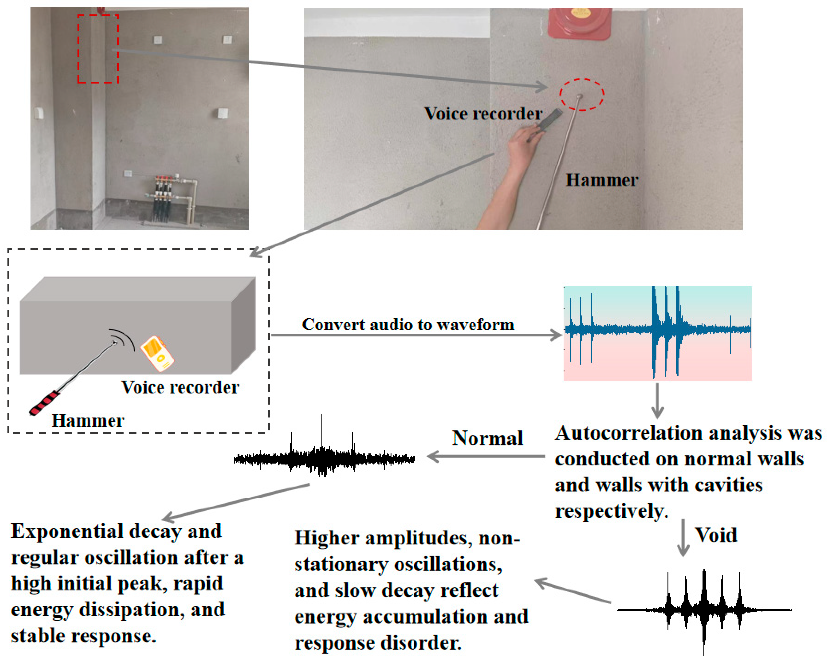
Figure 1 presents a complete schematic diagram of the acoustic identification experimental setup for concrete wall cavity detection, illustrating the core components, signal acquisition workflow, and data analysis process of the proposed method. Along with this schematic, on-site photographs of the actual test setup are supplemented in the revised manuscript, including the percussion hammer, digital voice recorder, and concrete wall specimens with precisely preset voids. The figure visually illustrates the physical components and spatial layout of the experimental system, emphasizing its structured and controlled approach. The core element is a concrete wall specimen, on which two distinct types of measurement points are clearly labeled: “normal” and “cavity.” The specimen incorporates precisely controlled preset voids, which are dimensionally regulated to realistically simulate typical field conditions, thereby ensuring the ecological validity of the experiment. The excitation system employs a standardized hollow hammer, whose mass and rubber-wrapped striking surface are designed to deliver consistent and repeatable impact energy with each strike, minimizing variability in the input excitation. For signal acquisition, a high-sensitivity digital voice recorder is utilized, strategically positioned perpendicular to the wall surface at a fixed distance of 10–15 cm from each striking point. This standardized positioning eliminates the influence of variable recording angles and distances on the signal amplitude, ensuring uniform acoustic recording conditions across all measurement locations. The schematic further delineates the complete signal pathway: once captured, the acoustic wave signals are recorded and converted into digital waveforms, then subjected to autocorrelation analysis separately for signals from normal walls and walls with cavities. Characteristic differences in the autocorrelation functions, such as the decay rate of the main lobe and the amplitude of side lobes, are extracted to form the basis for quantitative identification of void defects. The integration of controlled specimen preparation, a standardized excitation mechanism, a fixed-geometry recording setup, and a defined data flow constitutes a methodologically rigorous framework. This comprehensive and systematic procedure significantly enhances the reliability and reproducibility of the collected acoustic data, serving as a fundamental guarantee for the scientific rigor of the experimental design [37].

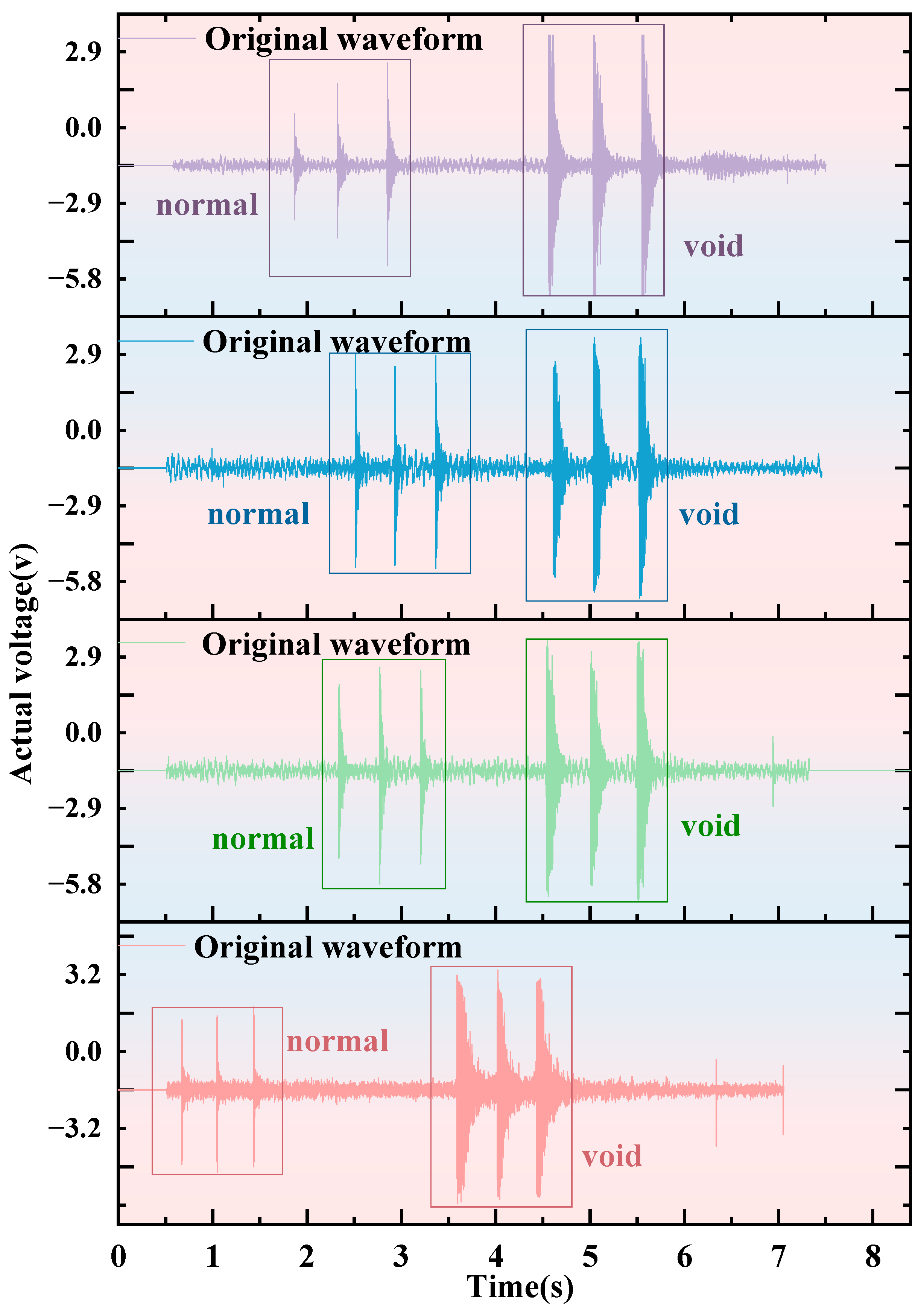
Figure 2 shows the original time-domain waveform diagrams of the concrete tapping sounds collected from four groups of measuring points. With time as the horizontal axis and sound pressure amplitude as the vertical axis, it intuitively presents the dynamic characteristics of the signals. By comparing the waveforms of the “normal” and “cavity” measuring points, significant differences can be observed. First, in terms of the signal amplitude, the “cavity” measuring points usually show a higher initial peak amplitude [38]. This is because the cavity within the concrete structure acts as a resonant chamber, trapping and reflecting the acoustic energy, which results in a more pronounced initial oscillation upon impact. The increased amplitude is visually evident across all four channels, with the void sections showing more pronounced peaks.

In contrast, the “normal” segments, representing the dense and homogeneous concrete areas, display lower peak amplitudes. This indicates that in intact structures, the impact energy is rapidly transmitted through the material and efficiently dissipated, leading to a damped response. Second, the differences in signal duration and attenuation patterns are particularly evident. The waveforms corresponding to the “void” condition display a prolonged decay, often characterized by a “tail-dragging” effect with sustained, low-frequency oscillations. This pattern reflects the acoustic reverberation and multiple internal reflections occurring within the enclosed air space of the void, which prolongs the vibration. Conversely, the “normal” waveforms are typically characterized by a sharp, impulsive profile. After the immediate initial peak, the amplitude decays rapidly and smoothly to the baseline, indicating efficient energy dissipation with minimal lingering vibrations in the solid, intact concrete matrix. The distinct “ringing” in void signals versus the “clean” decay in normal signals is a key visual differentiator. These observable time-domain features—the peak amplitude, the decay rate, and the overall signal duration and oscillation pattern—constitute the primary layer of physical evidence for distinguishing void from non-void conditions. They provide a clear and direct physical basis for the subsequent autocorrelation analysis. The autocorrelation function will further quantify these distinctive temporal signatures, particularly the periodicity and decay rate inherent in the “tail-dragging” effect of void signals, to establish a robust, objective, and quantifiable criterion for defect identification, moving beyond qualitative waveform observation.

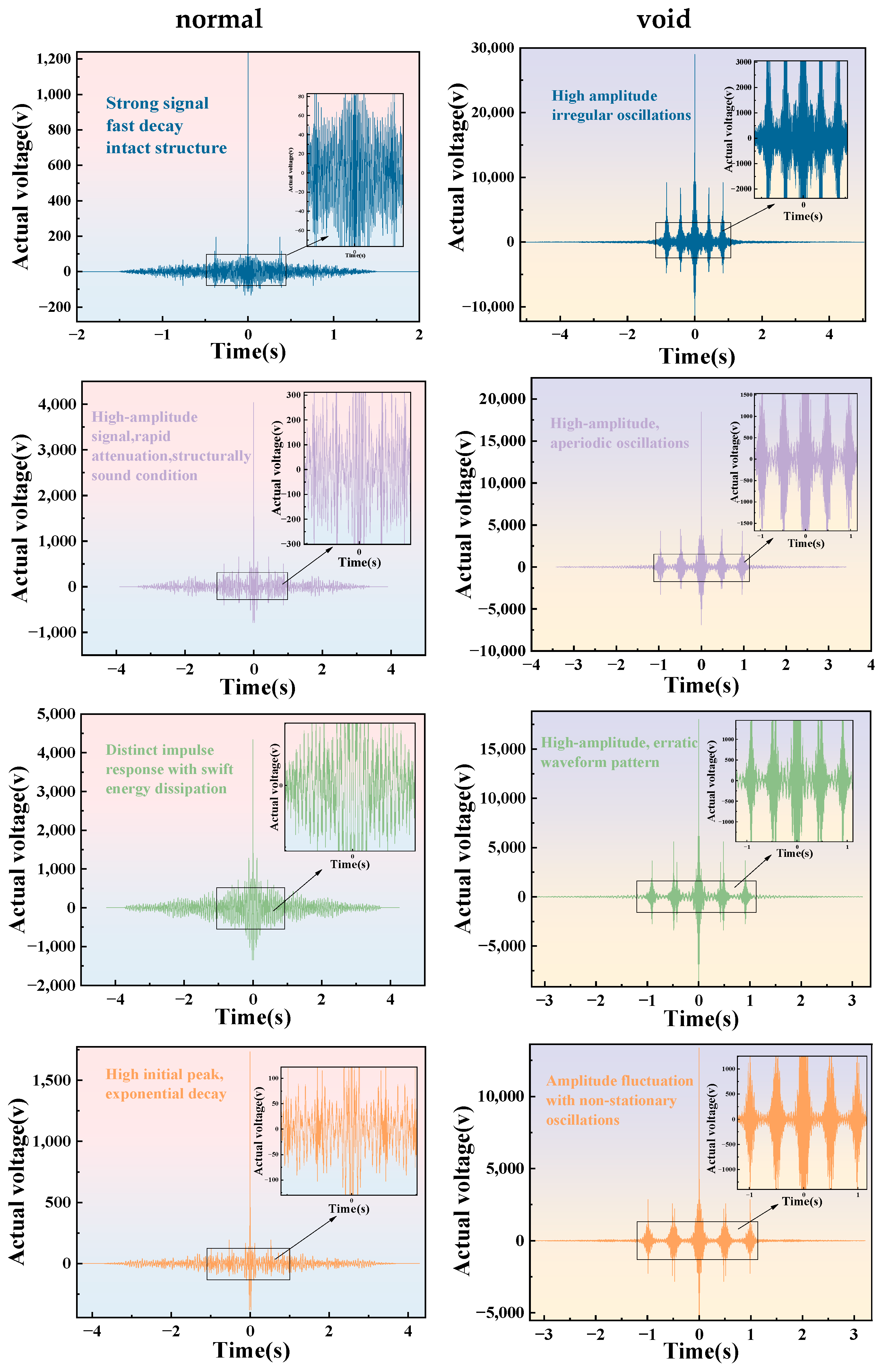
Figure 3 presents a systematic comparative analysis of the autocorrelation functions (ACF) for acoustic signals obtained from normal and cavity regions, visualized across four experimental trials in a two-by-four subplot arrangement. The horizontal axis uniformly represents the time delay τ (in seconds), while the vertical axis denotes the normalized correlation coefficient, enabling an in-depth, quantitative exploration of each signal’s internal temporal dependency and periodic structure [39]. The raw acoustic signal is collected in the form of electrical voltage, but all data are normalized before analysis; thus, the vertical axis does not represent raw voltage value, but a dimensionless normalized correlation coefficient. The layout is intuitively organized: the left column of subplots displays the ACF results from normal measurement points, while the right column corresponds to results from cavity points. This side-by-side, multi-trial presentation allows for immediate visual assessment of both intra-condition consistency and inter-condition divergence, significantly strengthening the observational validity.

A fundamental and consistent dichotomy in ACF morphology is unequivocally demonstrated across all trials. For signals originating from normal, structurally integral concrete (left column), the ACF curve exhibits a characteristic profile: it reaches an absolute maximum at τ = 0, representing perfect self-similarity, and subsequently undergoes a rapid, near-exponential decay to the baseline. This sharp decay pattern indicates that the acoustic signal possesses minimal temporal “memory” and lacks sustained periodic components. This mathematical characteristic is the direct correlate of the transient, impulsive “fast decay” nature observed in the original time-domain waveforms for normal points, confirming efficient energy dissipation within a homogeneous, dense medium.

In stark contrast, the ACF’s derived from cavity points (right column) reveal a profoundly different behavior. Following the central peak at τ = 0, the function decays at a markedly slower rate, exhibiting a prolonged, step-like decline. The most diagnostically salient feature is the consistent emergence, in the region where τ > 0, of a series of well-defined, periodic sidelobe peaks. These oscillatory peaks are a direct mathematical manifestation of the acoustic reverberation and multiple internal reflections occurring within the enclosed air space of a void. They precisely quantify the “ringing” or resonant persistence visually noted as prolonged oscillation in the original cavity waveforms. The presence and regularity of these sidelobes transform a qualitative auditory impression into an objective, measurable periodic signature.

In summary, the autocorrelation analysis effectively translates subjective waveform observations into robust, quantitative descriptors. The decay rate of the ACF envelope and the presence, amplitude, and periodicity of sidelobe peaks together constitute a reliable, dual-indicator framework for the objective identification of subsurface voids. Furthermore, the specific attributes of these sidelobes—such as their frequency and attenuation—provide a promising foundation for subsequent research aimed at correlating these signal features with physical void parameters like size, depth, and morphology, thereby advancing the methodology from mere detection towards quantitative characterization. The classification thresholds were determined based on the statistical distribution of characteristic parameters from repeated tests, and verified using cross-validation with independent samples to ensure reliability and accuracy.

Presented in Figure 4 are the amplitude-frequency response characteristics of normal and dense walls under acoustic excitation, consisting of four “amplitude-frequency” curves arranged from bottom to top. Observing the overall shape, the four curves exhibit a highly consistent pattern: starting from an amplitude baseline of about 16 at 0 Hz and increasing to 8000 Hz, the amplitude shows an almost perfectly linear growth trend, eventually stabilising at an amplitude of about 41. This smooth, monotonic response pattern contrasts sharply with the dramatic fluctuations and discrete peaks observed in the cavity wall spectrum. Specifically, throughout the entire analysis frequency band from 0 to 8000 Hz, none of the curves display sharp resonance peaks, harmonic sequences, or broad amplitude platforms. Even when closely examining the details through a local magnification frame, the amplitude variation trajectory remains continuous and stable, with no abrupt spikes or deep troughs, indicating that the acoustic energy is uniformly absorbed and dissipated by the wall material during propagation, without encountering internal interfaces that could cause strong local reflections or energy accumulation.

This straight linear spectral feature is essentially the standard response of a uniform, continuous medium to broadband acoustic excitation. It reveals the integrity of the internal structure of a normal wall: due to the absence of cavities, cracks or delaminated surfaces, sound waves cannot form resonant standing waves at specific frequencies, nor can they produce complex reverberation superpositions through multiple reflections. Therefore, the distribution of acoustic energy with frequency is determined solely by the material’s intrinsic damping and the geometric attenuation of wave propagation, manifesting as a simple linear relationship as shown in the figure. This set of curves together forms a key acoustic ‘baseline’ or reference template. In engineering diagnostics, by comparing the measured amplitude-frequency spectrum of a wall to this baseline, any deviation from the linear trend, particularly the occurrence of abnormal amplitude peaks in specific frequency bands, can be rapidly identified, providing direct and reliable acoustic evidence for determining whether hidden defects exist within the wall. The spectrum clearly confirms the nature of the acoustic response of a normal wall—a uniform, predictable energy decay process without resonance interference.

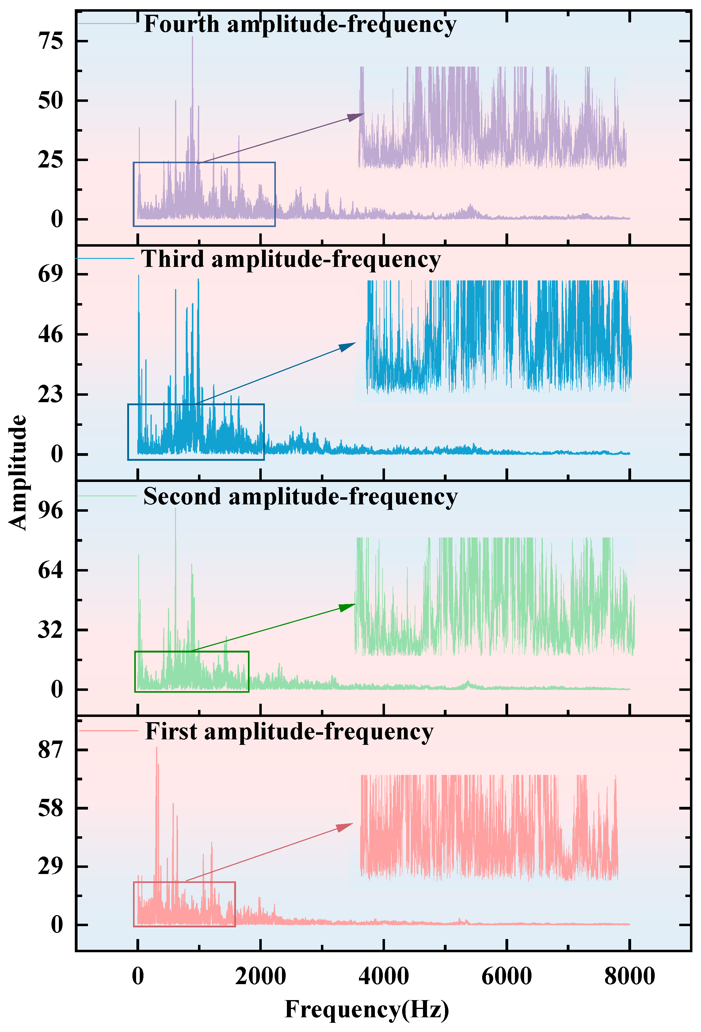
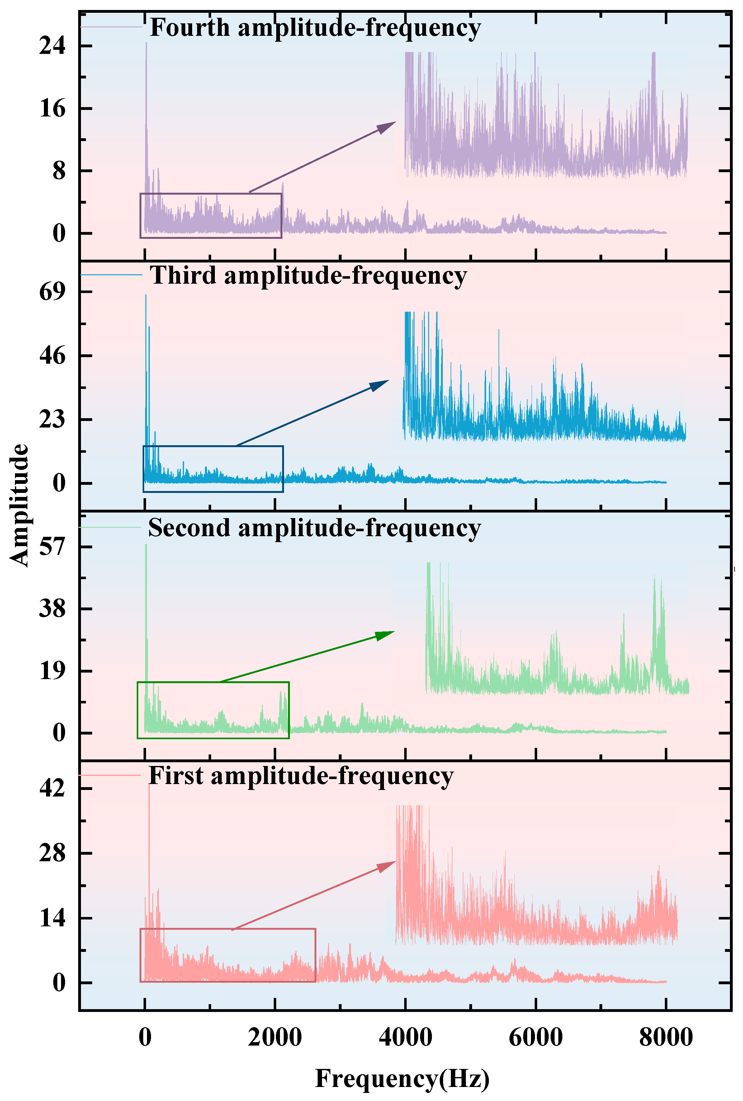
As shown in Figure 5, based on the analysis of the four sets of amplitude spectra in this figure, the acoustic signals in the void area of the concrete wall exhibit significant differences and commonalities in the frequency domain characteristics. From the ‘First amplitude-frequency’ to the ‘Fourth amplitude-frequency’, the spectra at all measurement points show relatively high baseline amplitude levels in the low-frequency range (especially below 500 Hz), indicating that the cavity structure generally amplifies low-frequency sound waves, mainly due to its be haviour as a Helmholtz resonator or similar cavity at the fundamental low-frequency resonance. Specifically, the ‘First’ and ‘Second’ amplitude-frequency spectra show sharp and prominent amplitude peaks in the low-frequency range (approximately 100–300 Hz), clearly indicating strong primary resonance modes in the cavity in this region with highly concentrated energy. The ‘Third’ and ‘Fourth’ amplitude-frequency spectra, although having relatively broader peaks in the low-frequency range, exhibit continuous and complex high-amplitude activity over a wider frequency band, particularly in the mid-to-high-frequency range (2000 Hz to 8000 Hz). Amplified details show that the ‘Third’ spectrum has a series of nearly equally spaced strong amplitude pulses in the 2000–4000 Hz frequency range, likely corresponding to a series of higher-order harmonic resonances or standing wave patterns determined by the specific dimensions of the cavity; while the ‘Fourth’ spectrum shows more dense and irregular spikes in the 1500–4000 Hz range, reflecting that the acoustic field at this measurement point is affected by more complex internal scattering, boundary irregularities, or local defects, resulting in multiple reflections and superposition of high-frequency acoustic energy. Overall, these spectra collectively confirm the resonant and reverberant nature of the cavity: the low-frequency peaks reveal its dominant resonant frequencies, while the broad and continuous amplitude response in the mid-to-high-frequency range reflects the repeated propagation and difficult dissipation of energy in the enclosed cavity, forming a complex reverberant field; this wideband energy distribution is a key indicator for identifying internal cavities and their acoustic characteristics in structures.

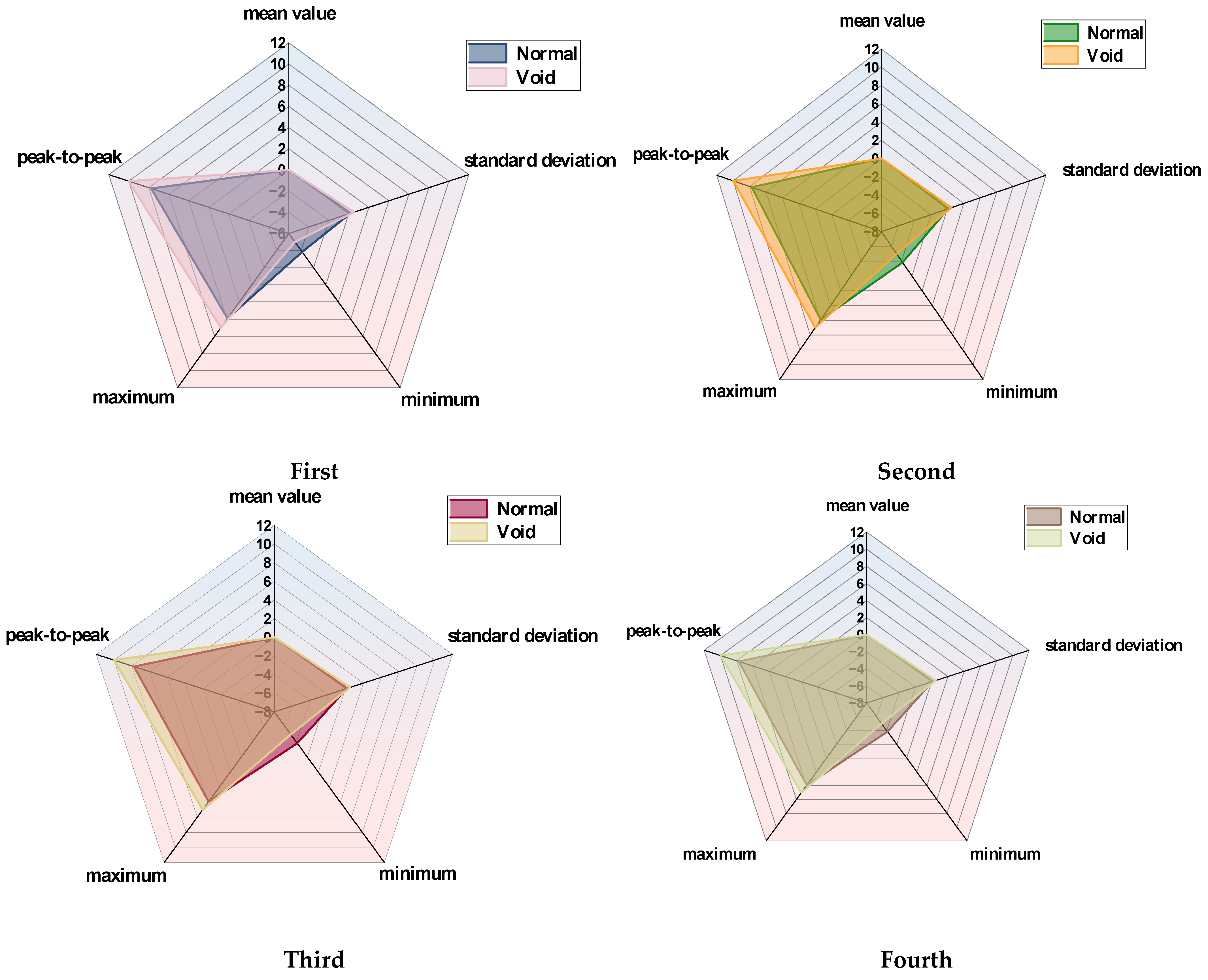
The four multidimensional radar charts arranged in two rows and two columns in Figure 6 visually compare the systematic differences in the time-domain statistical features of acoustic signals between “Normal” and “Void” wall types. Each radar chart includes five core statistical dimensions: mean value, peak-to-peak, standard deviation, maximum and minimum, forming a pentagonal evaluation framework, with all scales radiating outward from 0 at the centre to a maximum value of 12. Categories are distinguished by colour in the figure, with the “Normal” group shown in blue, its radar chart outline appearing smaller and more regular across the subplots; the “Void” group is shown in orange, with outlines generally showing larger and more irregular polygons.

From an overall trend analysis, the radar chart profile of the ‘Void’ group is significantly larger and differently shaped than that of the ‘Normal’ group across all four subplots. Specifically, in the two dimensions representing signal fluctuation intensity, ‘peak-to-peak’ and ‘standard deviation’, the metrics of the ‘Void’ group are far higher than those of the ‘Normal’ group, directly reflecting that the acoustic signals collected from cavity walls fluctuate more drastically and have a wider range of energy variation. At the same time, in the ‘maximum value’ dimension, the ‘Void’ group also generally shows higher figures, indicating the presence of stronger instantaneous pulses or high-amplitude components in the signal. These characteristics perfectly correspond to the physical processes of complex reflection, resonance, and reverberation generated by sound waves within the cavity. As a discontinuous interface, the cavity significantly enhances signal variability and extreme values. In contrast, the ‘Normal’ group exhibits relatively concentrated and lower figures across all dimensions, with a profile close to a small pentagon at the centre, reflecting that the sound signals from solid walls are more stable and uniform, with concentrated energy and limited fluctuation range.

In summary, this radar chart combination convincingly demonstrates that by extracting simple time-domain statistical features of the acoustic signals (such as peak-to-peak value, standard deviation, etc.) and visualising them using radar charts for comparison, it is possible to clearly and effectively identify walls with cavity defects from normal walls, providing an intuitive multi-dimensional basis for non-destructive testing.

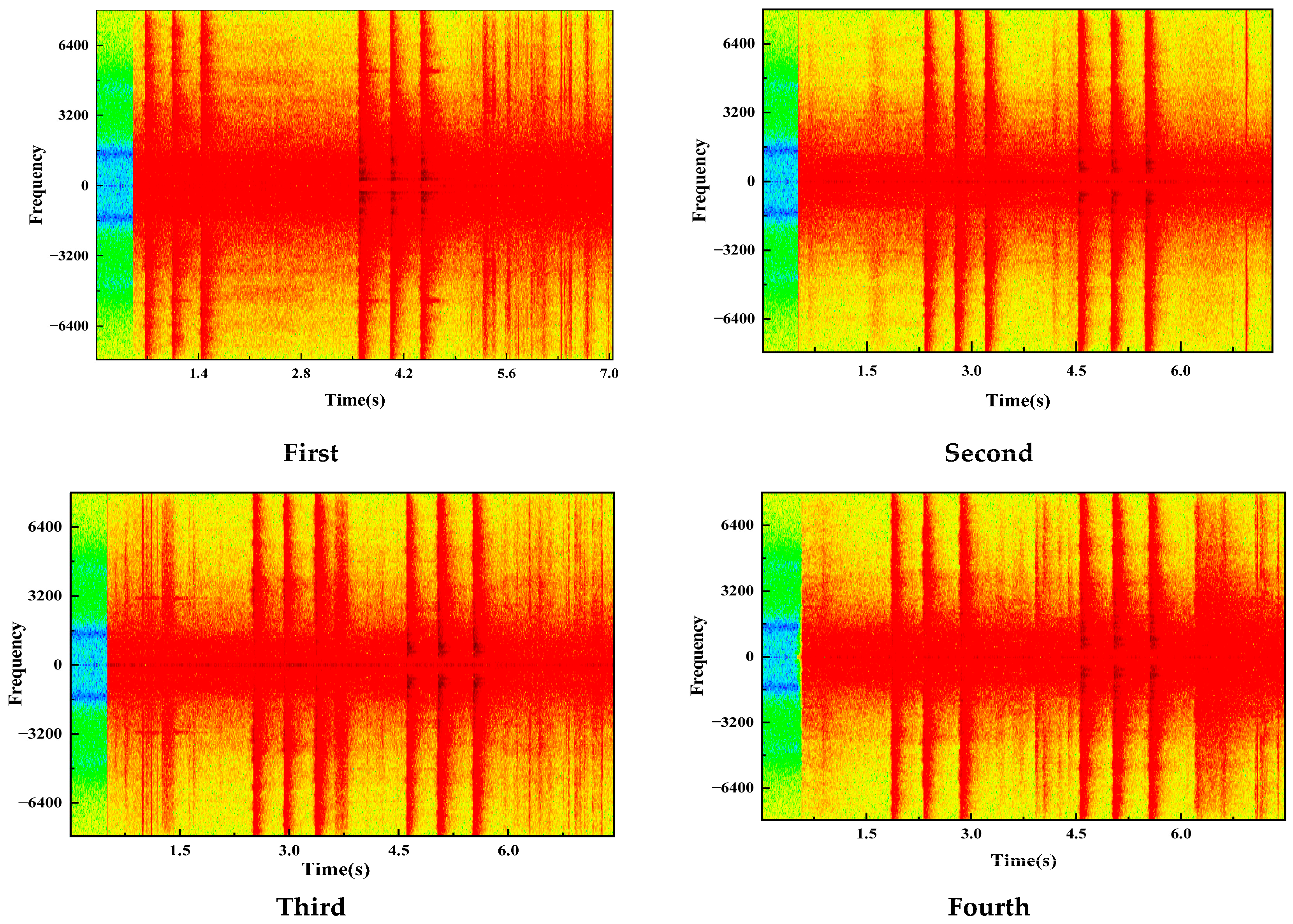
The four time-frequency spectrograms presented in Figure 7 are intended to compare and analyse the significant differences in the acoustic responses between a normal wall and a wall containing internal cavities in the time-frequency domain. Considering the overall layout and colour distribution, the vertical axis (frequency axis) range of all subplots is labelled as −6400 to 6400 (presumably in hertz), with the zero-frequency line positioned in the middle. The horizontal axis (time axis) ranges differ slightly, with the top-left subplot spanning 1.4 to 7 s and the other three spanning 1.5 to 6 s, suggesting this may be an analysis of data of varying durations or from different measurement points. The colour mapping of the time-frequency spectrogram clearly reflects the signal’s energy density, transitioning from low-energy green and cyan to high-energy yellow, orange, and bright red, thereby revealing the signal’s time-frequency structure.

In terms of the core characteristics of energy distribution, the four spectrograms exhibit highly similar but detailed variations in their patterns. The main portions of all spectrograms (after approximately 2 s) are dominated by large areas of bright red and yellow, with energy primarily concentrated in the mid-low frequency range (roughly between −3000 and 3000 Hz), indicating that whether it is a normal wall or a cavity wall, most of the acoustic energy is concentrated in this frequency band, consistent with the physical characteristics of typical structural sound propagation. However, careful observation reveals key differences: in spectrograms that may represent the presence of cavities (particularly possibly corresponding to the lower-left or lower-right subplots), the high-energy red areas display a more irregular, ‘fragmented’ patch-like distribution, and the continuity along the time axis shows abrupt changes or interruptions; meanwhile, in the higher frequency regions (near ±6400 Hz), scattered but distinct yellow or orange energy clusters can be seen, suggesting an enhancement of high-frequency components. In contrast, the spectrograms of normal walls (possibly corresponding to the upper-left or upper-right subplots) show that the contours of the high-energy areas (red) are generally smoother and more continuous, with a more uniform and stable temporal distribution, while the high-frequency energy diminishes more rapidly, predominantly displaying blue and green colours.

In addition, all spectrograms at the initial moment (approximately 1.4–2.0 s) show a vertical colour band extending from top to bottom, with the colour rapidly transitioning from green and cyan at the top to yellow at the bottom and blending into the main red area. This likely corresponds to the initial incident or transient response stage of the acoustic excitation signal, which contains a wide range of frequency components. The initial colour band on the cavity wall often exhibits more complex colour transitions or more pronounced energy variations at the lower end (near the zero-frequency region) where it meets the main red area, which may reflect the complex reflections and mode conversions generated when the sound waves encounter the cavity interface. In summary, this set of time–frequency spectra clearly reveals the differences in wall internal structure by comparing the uniformity of energy distribution on the time–frequency plane, the activity of high-frequency components, and the complexity of transient responses: the presence of a cavity leads to uneven energy distribution in the acoustic response, richer high-frequency components, and more complex time-varying characteristics, whereas a normal wall shows concentrated energy, smooth distribution, and regular attenuation patterns. This visual analysis provides an intuitive time–frequency basis for structural non-destructive testing using acoustic methods.

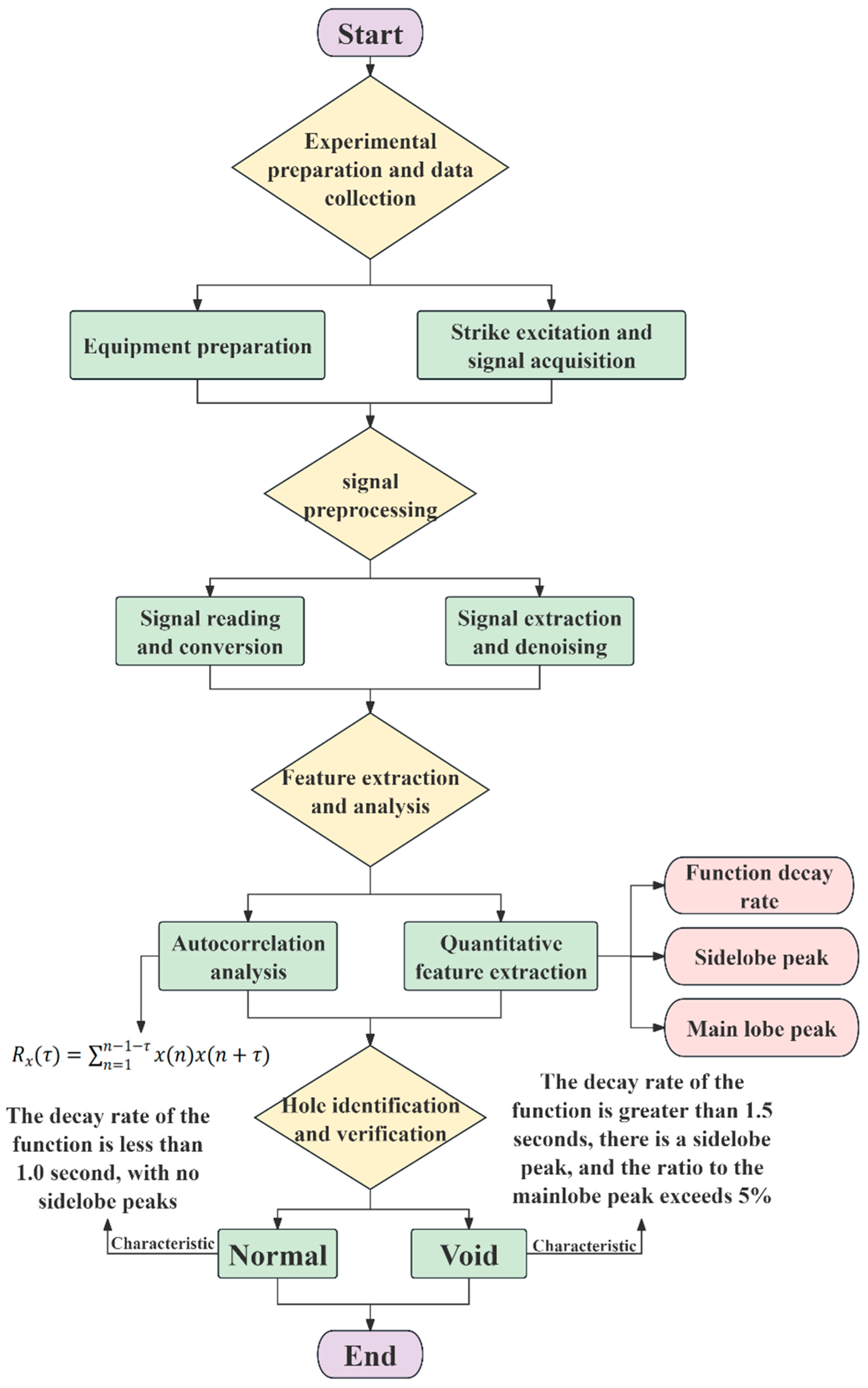
The flowchart in Figure 8 systematically delineates the complete technical pathway and implementation sequence for the non-destructive testing method of concrete cavities based on acoustic signal autocorrelation, as developed in this study. The entire procedure, structured in a clear, top-down linear format, is logically coherent and tightly interconnected, comprising four core operational stages: experimental preparation and data collection, signal pre-processing, feature extraction and analysis, and final cavity identification and verification.

Each stage is visually demarcated by specific geometric symbols—diamond-shaped decision boxes and rectangular process boxes—connected by directional arrows, providing an intuitive overview of the methodological workflow from initiation to conclusion. The first stage, “Experimental Preparation and Data Collection,” forms the empirical foundation of the research. The flowchart specifies that this phase involves the preparation of two distinct types of concrete wall specimens: a “normal wall” with a dense, homogeneous internal structure and a “cavity wall” with artificially preset, controlled void defects. Using a standardized percussion device (a rubber-wrapped hollow hammer) and a high-fidelity digital recorder, original acoustic signals are systematically collected under controlled environmental conditions. This rigorous approach ensures the reliability, consistency, and comparability of the raw data across all test scenarios. The second stage, “Signal Preprocessing”, is the bridge connecting the original data and advanced analysis. The figure shows that the collected analog sound signals are converted into digital signals through analog-to-digital conversion (sampling frequency: 16 kHz) [40]. This step transforms the physical sound waves into discrete digital time-series data, suitable for subsequent computational analysis. Further preprocessing, such as band-pass filtering and amplitude normalization, is applied to enhance signal quality and minimize the influence of ambient noise, thereby preparing a clean dataset for feature extraction. The third stage, “Feature Extraction and Analysis,” represents the core analytical innovation of this study. The flowchart emphasizes that the preprocessed digital signals are subjected to autocorrelation analysis. From the resulting autocorrelation function (ACF), key quantitative features are extracted. These primarily include the decay rate of the function envelope and the presence, amplitude, and periodicity of any sidelobe peaks. This process effectively translates observable acoustic phenomena (like reverberation) into objective, computable mathematical indicators, moving beyond qualitative assessment. The fourth and final stage, “Cavity Identification and Verification,” demonstrates the practical application and validation of the method. Based on the extracted quantitative features, the flowchart illustrates the establishment of clear classification criteria. For instance, a signal exhibiting a function decay rate of less than 1.0 s with no significant sidelobe peaks is classified as originating from a Normal wall. Conversely, a signal with a decay rate exceeding 1.5 s, coupled with the presence of sidelobe peaks whose amplitude exceeds 5% of the main lobe, is classified as indicating a Void. The accuracy of this automated identification is subsequently verified by comparing the algorithmic outputs with the known, actual states of the specimens, thereby validating the efficacy and reliability of the proposed technical route.

4. Discussion

Although all experiments were carried out in a quiet and controlled laboratory environment, potential measurement errors and uncertainties were quantitatively analyzed to ensure the reliability of the experimental results. The main sources of uncertainty include slight fluctuations in tapping force and angle, minor deviations in the position and orientation of the recorder, residual environmental background noise, and numerical errors introduced by signal filtering and amplitude normalization. Based on repeated tests at the same measurement points, the coefficient of variation (CV) and 95% confidence interval were calculated for key characteristic parameters, including the main lobe decay rate and side lobe amplitude ratio of the autocorrelation function. The results show that the relative error of these parameters is controlled within ±5%, indicating good repeatability and stability of the proposed method. The quantitative error analysis confirms that the observed differences between normal and cavity walls are statistically significant and not caused by measurement uncertainty, thus enhancing the credibility of the experimental data.

Table 1. Comparison of different concrete wall cavity detection methods.

Detection Method	Advantages	Limitations
Traditional tapping	Fast, simple, low-cost	High subjectivity, low stability, non-quantitative
Ultrasonic testing	High precision, mature technology	Expensive, requires coupling, complex operation
Impact-echo method	Effective for deep defects	Slow, low efficiency, Professional operation needed
Infrared thermography	Non-contact, large-area screening	Easily affected by temperature, environment
Proposed method	Objective, quantitative, anti-interference, fast	More suitable for rapid screening

compares the proposed method with four common concrete wall cavity detection methods, including traditional tapping, ultrasonic testing, impact-echo method, and infrared thermography [17,41].

The experimental results show that obvious differences exist in time-domain waveforms, amplitude-frequency characteristics, time-frequency distributions, and autocorrelation function characteristics between intact concrete walls and those with cavities [41]. From the perspective of mathematical description, the autocorrelation function can effectively extract the periodic components and attenuation laws of tapping signals. The decay rate of the main lobe, the amplitude and period of side lobes, and the energy distribution stability of the signal can be used as key quantitative parameters to identify cavity defects. These parameters are not affected by subjective human factors and can realize objective and stable recognition.

From a practical point of view, these quantitative characteristics form a new set of scientific and theoretical knowledge for on-site detection [17,42]. Traditional methods rely on subjective experience, while the proposed method uses signal amplitude distribution, stability, and autocorrelation characteristics to establish a clear judgment basis, which provides a theoretical basis for converting manual listening into instrument-based quantitative detection.

Compared with other methods, the proposed method does not require expensive equipment or complex operation. It can maintain high stability in actual engineering environments and has strong anti-interference ability. It can meet the needs of large-scale, rapid, on-site screening of wall cavities, and provides a reliable auxiliary means for structural safety inspection.

In summary, the method establishes a quantitative relationship between acoustic signal characteristics and cavity states based on autocorrelation theory. It not only has clear scientific contributions in mathematical description and signal analysis but also has important practical value in engineering applications such as construction acceptance, existing building detection, and hidden danger investigation [41,42].

5. Conclusions

This study systematically investigates the acoustic response characteristics of concrete walls by comparing intact and hollow specimens, and identifies consistent and distinguishable patterns in the autocorrelation function (ACF) of tapping signals. Specifically, signals from intact walls exhibit a high main lobe, rapid decay, and negligible side lobes, whereas signals from hollow walls show a high main lobe, slow decay, and distinct periodic side lobes; these differences are reliably verified across four independent tests. By focusing on the temporal structure of acoustic signals rather than conventional time-domain amplitude or frequency features, this work mathematically quantifies the traditionally subjective method of “listening for hollows,” thus reducing the influence of tapping force inconsistency and operator experience. The proposed autocorrelation-based approach exhibits improved immunity to environmental noise and higher sensitivity to small-scale defects.

From the perspectives of mathematical representation and engineering application, this study obtains reliable quantitative results and establishes a theoretical foundation for cavity detection. The autocorrelation function is adopted to characterize the temporal correlation and attenuation law of tapping signals, where the main lobe decay rate, side lobe amplitude, and periodicity are extracted as stable quantitative indicators. The amplitude distribution and energy stability of tapping signals are closely correlated with the internal state of concrete walls: a concentrated and stable amplitude distribution indicates a solid structure, while a discrete and prolonged response indicates the presence of a cavity. These quantitative parameters transform subjective manual listening into objective, repeatable criteria independent of personal experience and environmental interference, providing a unified judgment basis for field detection and supporting the development of intelligent, quantitative non-destructive testing tools for concrete structures.

Overall, the proposed method fills the gap between empirical detection and objective quantitative analysis, providing a reliable and advanced technical framework for structural health monitoring. The differences in side lobe characteristics also imply a potential correlation with cavity geometry, which can support further research on refined defect evaluation. Featuring low cost, simple operation, quantitative analysis, and high efficiency, the method has broad application prospects in the rapid on-site inspection of concrete wall cavities in residential buildings, commercial buildings, bridges, and tunnels. It can assist engineers in quickly locating defects, evaluating structural quality, and making timely maintenance decisions, offering important technical support for structural safety assessment, digital management, and intelligent detection in the construction industry.