Article

Prediction on Slip Modulus of Screwed Connection for Timber–Concrete Composite Structures Based on Machine Learning

1
College of Civil Engineering, Nanjing Tech University, Nanjing 211816, China
2
College of Materials Science and Engineering, Nanjing Forestry University, Nanjing 210037, China
*
Author to whom correspondence should be addressed.
Buildings 2025, 15(14), 2458; https://doi.org/10.3390/buildings15142458
Submission received: 2 June 2025 / Revised: 7 July 2025 / Accepted: 11 July 2025 / Published: 13 July 2025
(This article belongs to the Special Issue Performance Analysis of Timber Composite Structures)

Abstract

Screwed connections are widely adopted in timber–concrete composite (TCC) structures. Owing to the diverse connection configurations and complex shear mechanisms, existing empirical models or theoretical formulas cannot accurately and efficiently predict the shear modulus of a screwed connection. Therefore, this study develops machine learning (ML) algorithms to accurately predict the slip modulus. A data set including 222 sets of testing results was established by collecting the values of the slip modulus and associated ten features. Four ML methods, including decision tree (DT), random forest (RF), adaptive boosting machine (AdaBoost), and gradient boosting regression tree (GBRT), are adopted to develop the ML algorithm. The Shapley Additive Explanation (SHAP) framework was employed to interpret the effects of related features on the slip modulus. GBRT demonstrated the best accuracy compared with the other three ML methods in terms of four popular quantitative metrics. Moreover, all ML methods showed an evident accuracy advantage compared to existing analytical methods. Through a SHAP analysis, it was found that concrete strength, screw inclination, timber density, and timber type have a large impact on the slip modulus of a screwed connection compared to other input features.

1. Introduction

Timber–concrete composite (TCC) structures consist of an upper concrete slab and a bottom timber member (beam or slab), as shown in Figure 1. The concrete slab and timber member are connected using shear connection systems. The TCC structure was initially formed for the restoration of old wooden buildings by introducing a concrete slab into the timber floor system [1]. In modern timber buildings, concrete slabs are applied to wooden floors to form TCC floor systems, aiming to improve the bending performance, fire resistance, and vibration performance of the floor system compared to a pure timber floor [2,3,4,5]. Compared with pure concrete buildings, TCC structures offer the advantages of low carbon emissions and high assembly efficiencies [6,7,8].
The shear connections are designed to provide a longitudinal restriction to constrain the relative slip and a vertical restriction to prevent the opening gap between the timber and concrete. The shear performance of shear connection is mostly evaluated by push-out tests, with a symmetric push-out specimen shown in Figure 1. Common connection methods mainly include screwed, notched-screw, and glued-in steel-plate connections [9,10,11,12,13,14]. Among them, the screwed connection achieved significant attention, owing to its excellent load-carrying capacity, good ductility, convenient processing, and low construction cost [9,15].
The typical screw arrangement approaches are depicted in Figure 2. Initially, screws were drilled vertically into the timber [16], as shown Figure 2a. The shear performance of a vertically screwed connector depends primarily on the timber foundation modulus and screw-bending performance [17]. The typical failure modes are timber embedment and screw-bending failures. Then, to improve the shear performance of a screwed connection, some studies [18,19,20] placed screws inclined in the direction of the load, as shown in Figure 2b, which is called a shear–tension screw connection, and achieved the expected improvements. This is because the superior pull-out behavior of the screw increases the shear performance of the shear–tension screw connection. As a bending member, a negative bending moment action may occur at the TCC member end or under the repeated action of seismic loads. Thus, the shear performance of an inverse inclined screw (shear–compression screw) connection shown in Figure 2c was also investigated [21,22], and it was demonstrated that its shear performance was inferior to that of the shear–tension screw connection. To satisfy the shear performance in two directions [23,24], the bidirectional screwed connection is also a commonly used connection method, as shown in Figure 2d.
The screwed connection is characterized by screw-bending yielding and timber embedment failures [25,26,27], demonstrating good ductility. Based on the European yield model, the calculation methods for the load-carrying capacity of each arrangement were established [18,26], and they were adopted in the latest design guidelines [15,28]. However, existing design standards and guidelines, such as FP 1402/WG 4 [15], Eurocode 5 [29], and Auclair [30], did not specify detailed rules for the calculation of the slip modulus of TCC screwed connections, owing to the different stress mechanisms of various screwed connection configurations.
Several analytical methods for predicting the slip modulus of TCC screwed connections have been proposed. There are some limitations to these models in terms of applicability and feasibility. For example, Di Nino et al. [31] obtained an analytical model of the slip modulus of an inclined screw connection with an interlayer by ignoring the interfacial friction between concrete and timber. However, the analytical model proposed by Di Nino [31] is a closed-form expression, and its calculation accuracy depends on the determination of the timber foundation modulus. Mirdad and Chui [32] also proposed a slip modulus prediction model for an inclined screwed TCC connection with a gap by determining the actual rotation positions of the screw in glulam, in which the timber embedment foundation stiffness and screw axial withdrawal stiffness were key parameters that needed to be determined through tests.
In recent years, machine-learning (ML) methods have become powerful tools for solving various engineering problems because they can extract useful patterns and insights from a large amount of information, reduce the risk of human error, and improve the consistency and reliability of the work [33]. Because of the advantages mentioned above, ML methods were applied to solve many structural problems [34], especially concrete-related ones [35,36,37].
As to the application of ML in timber fields, existing studies mainly focused on the physical properties of wood material, such as its time-dependent responses, moisture content variations, and hygro-thermal behaviors [38,39,40,41]. In particular, attempts applying ML methods to TCC structures have not been reported. This study aims to establish ML algorithms and evaluate their feasibility and accuracy in predicting the slip modulus of the TCC screwed connection and to utilize the Shapley Additive Explanation (SHAP) framework [36] to interpret the effects of related features on the slip modulus of TCC screwed connections.
This article employs four popular ML methods—decision tree, random forest, AdaBoost, and gradient boosting regression tree—to provide a prediction of the slip modulus of TCC screwed connections. This study mainly includes four parts: (i) the collection of push-out testing results and the establishment of a data set, (ii) the introduction of the ML methods adopted, (iii) the ML prediction accuracy analysis and SHAP interpretation, and (iv) a comparison of design methods in existing standards and the latest academic research. In addition to the accuracy prediction, the work in this study provides a reference for further improvements in related design methods for screwed connected TCC structures.

2. Establishment of Experimental Data Set

2.1. Introduction of Interfacial Shear Tests for TCC Structures

The interfacial shear performance of TCC screwed connections was evaluated using single or double shear tests. The double shear test on TCC shear connections was conducted mainly by adopting the loading diagram (see Figure 3a) and procedure (see Figure 3b) regulated in EN 26891 [42]. Ling et al. [43] compared the effects of test configurations (single and double shear tests) on the slip modulus of TCC shear connections, and they found that the test configuration has no obvious regular effect on the slip modulus. Therefore, the experimental results based on both single and double shear tests were collected to establish the slip modulus data set in this study. The relative interfacial slip in the middle of the connection region was measured to calculate the slip modulus. The slip modulus of the screwed connection in the serviceability limit state (SLS) was calculated using Equation (1), according to EN 26891 [42], which was used to calculate the bending stiffness of TCC beams and floors in the SLS.
K s = 0.4 F est 4 3 ( s 0.4 s 0.1 )
where Fest denotes the estimated capacity, which is determined through a preliminary test or theoretical prediction and should be corrected when the error compared to the actual maximum test load is larger than 20%; s0.4 and s0.1 represent interfacial slip when the loads are 0.4Fest and 0.1Fest, respectively, at the first loading cycle, as shown in Figure 3b.

2.2. Data Set Processing and Determination of Input Parameters

2.2.1. Data Set Collection

Based on the knowledge of the slip performance of TCC structures, experimental results using TCC screwed connections were collected. Considering the potential characteristic parameters input in ML models, the articles cited in this study provided explicit information about slip modulus test values in SLS, material properties, and geometric configuration parameters. Based on this requirement, 222 sets of experimental data were extracted from 17 studies [18,21,22,26,44,45,46,47,48,49,50,51,52,53,54,55,56] to form the data set. Moreover, all experimental values were adopted by being unified as the slip modulus values provided via a pair of screws in the data set because the bidirectional screwed connection (see Figure 2d) consists of at least two screws.

2.2.2. Determination of Input Features

Many researchers focused on the effects of different features on the slip modulus of screwed connections. Based on the overview of the related investigations [18,21,22,26,31,32,44,46,47,48,49,50,51,52,53,54,55,57], 10 features were determined. First, two typical screw arrangement (SA) methods, including unidirectional and bidirectional screws, were considered, as shown in Figure 2. As shown in Figure 2a–Figure 2c, the unidirectional screw connection includes vertical, shear–tension, and shear–compression screwed connections, respectively.
In addition to SA, the determined input features include the screw diameter, ds, in mm, the screw penetration length in timber, ls, in mm, the screw inclination angle, α, in °, the screw type (ST), the timber density, ρt, in g/cm3, the timber type (TT), the interlayer (plywood) thickness, ti, in mm, the concrete strength, fc, in MPa, and the concrete type (CT). The relevant parameters are depicted in Figure 2.
Under ST, hexagonal head screws and self-tapping screws are considered. Under TT, glued laminated timber (GLT), laminated veneer lumber (LVL), cross-laminated timber (CLT), and composite lumber panel (CLP) are considered, among which CLP is made of lumber and structural composite lumber [58]. CT includes normal concrete (NC) and light-weight aggregate concrete (LWAC).

2.3. Processing and Correlation Analysis

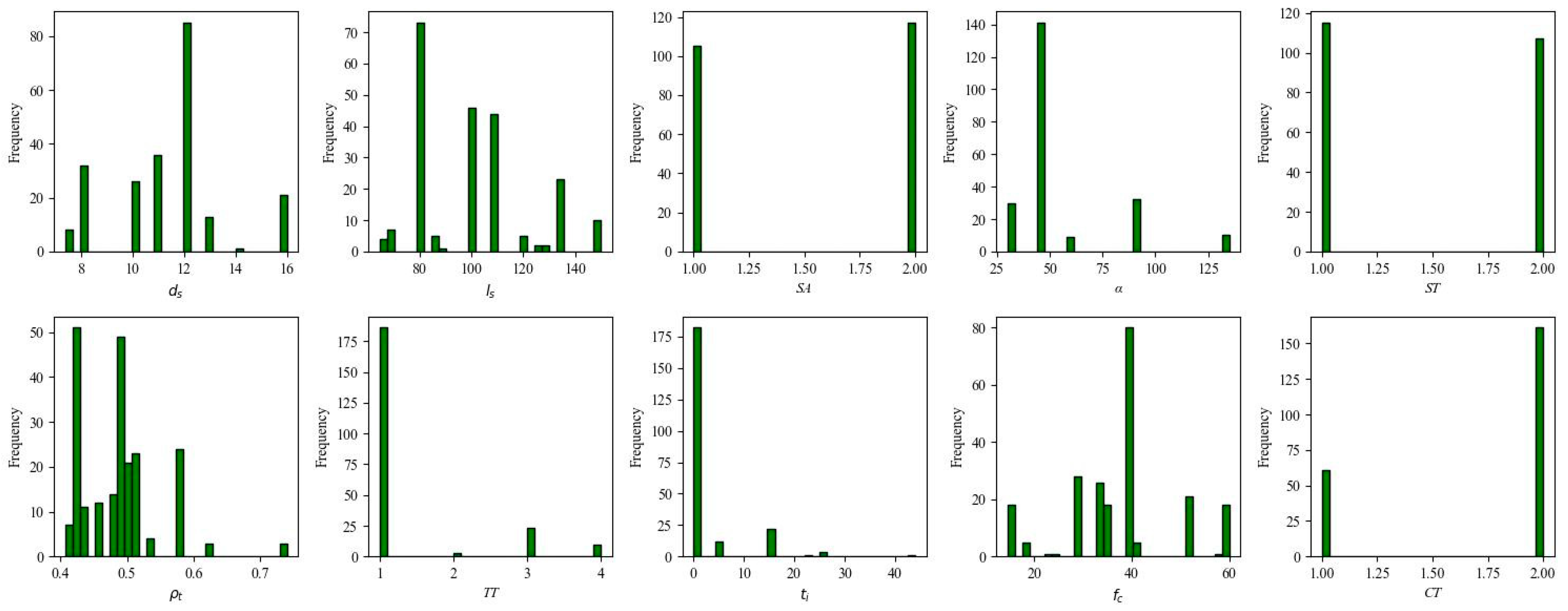
Figure 4 shows the frequency of ten features for the collected data set. In the ML algorithm routine, the experimental data in the data set must be preprocessed to facilitate the use of the model for mathematical model classification and regression calculation. For the features of ds, ls, α, ρt, ti, and fc, the actual values of the corresponding physical variables are adopted in the data set. As to the feature SA, the unidirectional screws are assigned as 1 when the bidirectional screws are 2. For the feature ST, the self-tapping screw is designated as 1 when the hexagon head screw is designated as 2. As to the feature TT, the reference symbols of GLT, LVL, CLT, and CLP are 1, 2, 3, and 4, respectively. For the feature CT, the reference symbols of LWAC and NC are 1 and 2, respectively.
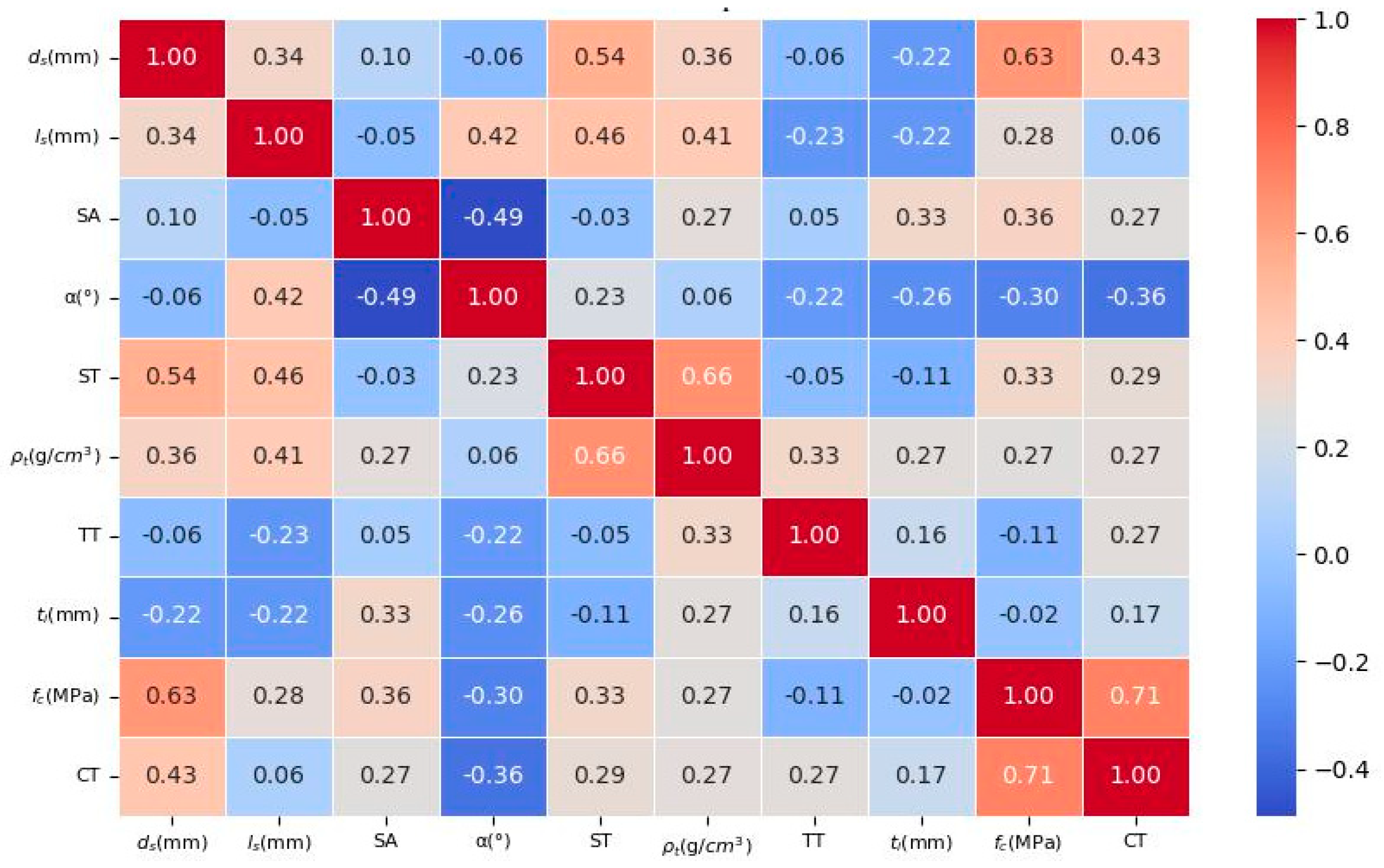
Figure 5 shows the correlation among the input features. There is a moderate correlation between screw diameter and screw types, with a correlation coefficient of 0.54. This is because the diameter of self-tapping screws mainly ranges from 6 to 13 mm, whereas that of the hexagonal head screws is 12–18 mm. The concrete type (CT) and fc have the highest correlation coefficient of 0.71. The NC essentially has a higher compression strength than LWAC. In addition, the screw diameter exhibits a moderate correlation coefficient of 0.63 with the concrete compressive strength. However, the authors believe the moderate correlation between the screw diameter and the concrete compressive strength seems to be coincidental.

3. ML Algorithms

3.1. ML Methods

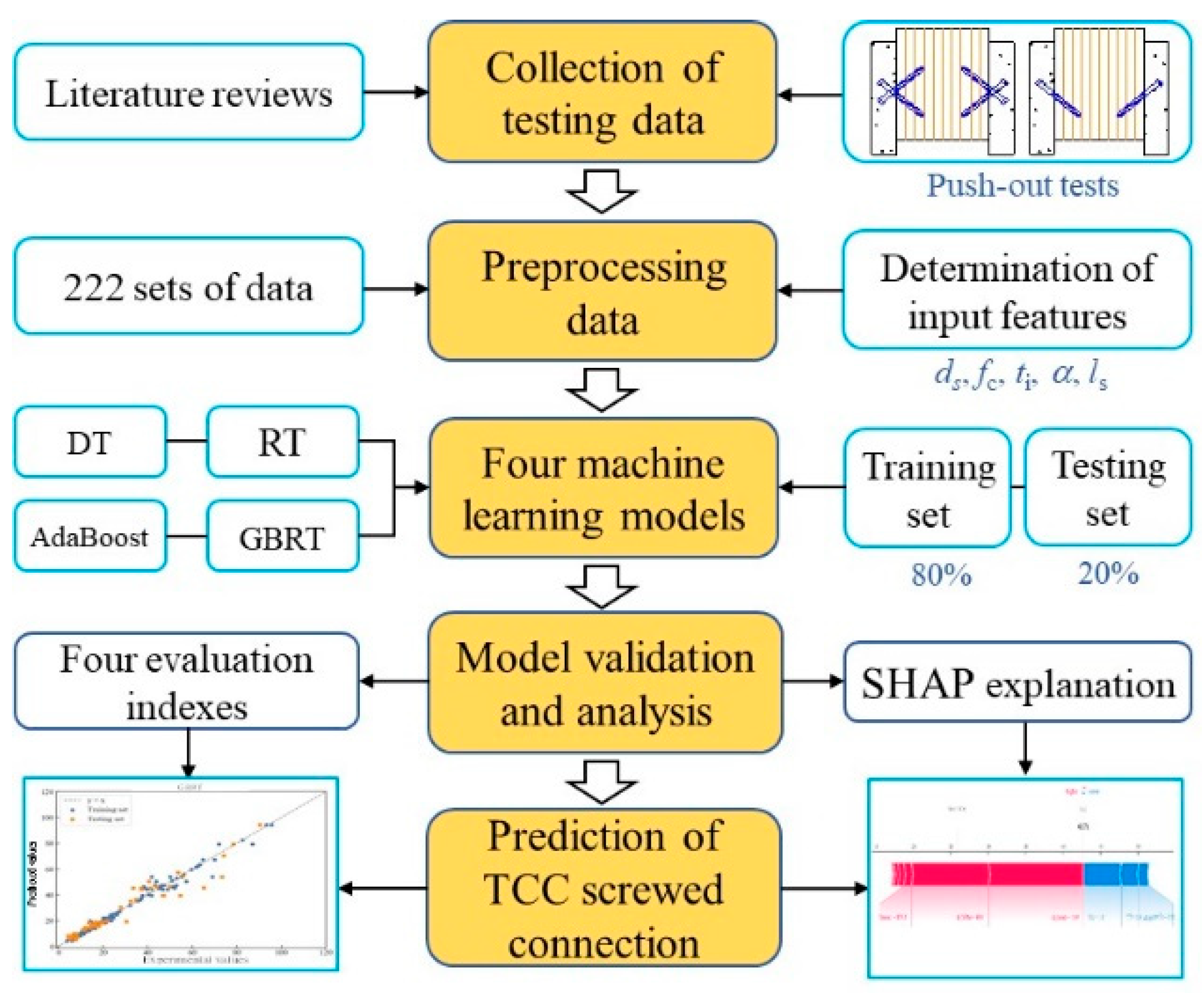
This study uses ML methods to develop an explainable model that can effectively predict the slip modulus of TCC screwed connections. As shown in Figure 6, the research process can be described as follows: (i) Establishing a data set based on experimental results from the existing literature; (ii) preprocessing existing experimental data and determining the input features; (iii) adopting four classical ML models, including DT, RF, AdaBoost, and GBRT, to predict the slip modulus of TCC screwed connections; (iv) validating the accuracy of ML models using four evaluation indexes; and (v) introducing SHAP to explain the effects of different parameters on the slip modulus of screw connections.

3.1.1. Decision Tree

A decision tree (DT) is an ML algorithm based on a tree structure for the classification and regression analysis of a data set [59]. The DT algorithm is characterized by good classification and generalization abilities [60]. In addition, each decision node of the DL algorithm relies only on partial features, rather than the entire data set. Therefore, the influence of local noise or outliers on the entire model is relatively small, resulting in the good robustness of the DT algorithm [61]. DT adopts the Gini index (GI), which is a measure of impurity, as the criterion to measure the feature selection [35]. The GI represents the probability that a randomly selected sample in the data set is misclassified, and it can be expressed as follows:
G I ( P ) = k = 1 K p k ( 1 p k )
where K denotes the total number of ‘classes’, and pk denotes the proportion of samples belonging to class k in the data set P.

3.1.2. Random Forest

A random forest (RF) is a classifier containing many DTs that can be used for both classification and regression problems, as well as dimension reduction problems [62,63,64,65]. It offers a significant advantage in processing massive and high-dimensional data and improving the prediction accuracy without significantly increasing the computational burden of the algorithm [66].
The general steps of RF are summarized as follows: A part of the samples and some of features are randomly selected from the training set, and a DT is constructed using the randomly sampled samples and features; the classification and regression tree (CART) algorithm is adopted to repeat the above steps several times, randomly selecting different samples and features each time to build multiple DTs. The final classification result for the classification task is determined through voting. Meanwhile, for the regression task, the average value of predicted results of all DTs is taken as the final prediction result [67].

3.1.3. Adaptive Boosting Machine

The adaptive boosting machine (AdaBoost) is a popular ensemble learning algorithm. Its core idea is to iteratively train multiple weak learners and weight them together to form a powerful learner [68]. The features of the AdaBoost algorithm mainly include the following [69,70,71]: (i) The AdaBoost algorithm can adaptively adjust the weight of samples. In each iteration, the algorithm adjusts the sample weight based on the prediction results of the previous weak learner. Subsequent weak learners pay more attention to those samples that are misclassified. (ii) The AdaBoost algorithm builds the final powerful learner by iteratively training weak learners. In each iteration, a new weak learner is added until a predetermined error rate or maximum number of iterations is reached. (iii) The weight of each weak learner is assigned according to its classification accuracy. The AdaBoost algorithm can be explained as follows:
H ( x ) = sign i = 1 n ω i h i ( x )
where H(x) denotes the results of a powerful learner, hi(x) is the predicted result for the i-th weak learner, n represents the number of weak learners, and ωi denotes the weight for the i-th weak learner.

3.1.4. Gradient Boosting Regression Tree

The gradient boosting regression tree (GBRT) method proposed by Fredman [72] offers significant benefits in solving classification and regression problems [73]. The procedure of GBRT are summarized as follows: (i) the GBRT algorithm starts by initializing a basic classifier [74]; (ii) it calculates the residual value of the previous term model using gradient descent method; (iii) it minimizes the loss function to obtain the root node value based on the former residual value, as shown in Equation (4); (iv) and it calculates the estimated result at the m-th RT. The final GBRT model can be obtained via Equation (5).
a m , j = argmin a , β i = 1 N [ r i ( m ) β h ( x i ; a ) ] 2
where am,j denotes the output parameter at the m-th iteration for the j-th feature unit, ri(m) is the residual of the fitting results at the m-th (m = 1, …, M) iteration for the i-th data (sample), β denotes the weight value of weak learners [75], h(xi; a) represents the RT function, and a represents the RT parameter.
F m ( x ) = m = 1 M j = 1 J a m , j I ( x R m , j )
where I = 1 for x R m , j , and otherwise, I = 0; R m , j denotes the feature space for leaf nodes at the m-th RT [74].

3.2. Quantitative Indices

To evaluate the accuracy of the adopted ML models, four quantitative indices are adopted: R-Squared (R2), the root mean squared error (RMSE), the mean absolute error (MAE), and the mean absolute percentage error (MAPE). All of these were adopted previously to assess the accuracy of various ML algorithms [68,76,77]. The higher the value of R2 or the lower the values for the other three indexes, the higher the prediction accuracy for ML algorithms. The formulas of the four indices are shown in Equations (6)–(9), respectively.
R 2 = 1 i = 1 n ( X i Y i ) 2 i = 1 n ( Y i Y ¯ ) 2
RMSE = i = 1 n ( X i Y i ) 2 n
MAE = i = 1 n X i Y i n
M A P E = 100 % n i = 1 n X i Y i Y i
where Xi and Yi are the predicted slip modulus and tested slip modulus, respectively; Y ¯ denotes the mean values of all the tested slip modulus, and n is the total sample number.

4. Development and Results of ML Models

4.1. Hyperparameter Tuning

For different data sets, the hyperparameters of each ML model are different, and the decision on the hyperparameters directly affects the prediction performance of the final model. Bayesian optimization is a popular hyperparameter optimization method widely used in various ML tasks. Hyperopt is a Python library for hyperparameter optimization that features a Bayesian optimization algorithm at its core. In this study, the Hyperopt library is used for each ML model, where a parameter space is defined and Bayesian optimization methods are used to automatically select the optimal combination of parameters for optimizing a given objective function.
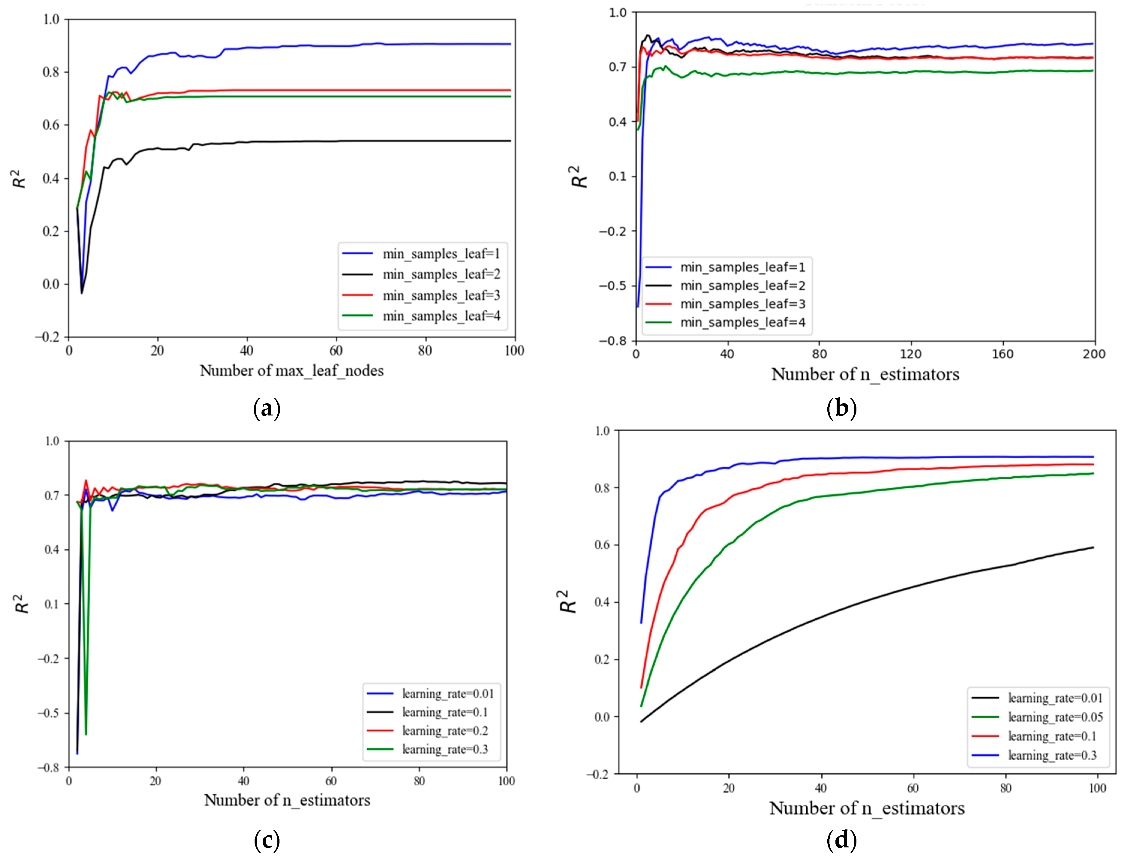
Figure 7 shows the influence of a hyperparameter on the prediction accuracy. In Figure 7a, it can be observed that the minimum sampling leaf significantly affects the prediction accuracy for the DT model. When the minimum sampling leaf is 1, R2 is stable at approximately 0.9. As shown in Figure 7b, with a decrease in the value of the minimum sampling leaf, the prediction accuracy of the RF model tended to increase. As to AdaBoost, the prediction accuracy tends to be stable when the learning rate is larger than 0.01. Figure 7d demonstrates that the R2 of GBRT tends to be stable with the increase in the tree. When the learning rate is 0.01, R2 tends to be stable at only 0.6. For comparison, consider that R2 reaches 0.9 when the learning rate is 0.3. Therefore, the hyperparameters of the ML model significantly affect the final performance of the model.
Through the parameter search method combined with the Hyperopt library and 10-fold cross-validation, the optimal hyperparameter combinations are determined for each ML model. The hyperparameter space and optimal hyperparameter combinations are listed in Table 1, and the optimal hyperparameters are used for model development.

4.2. Prediction Accuracy

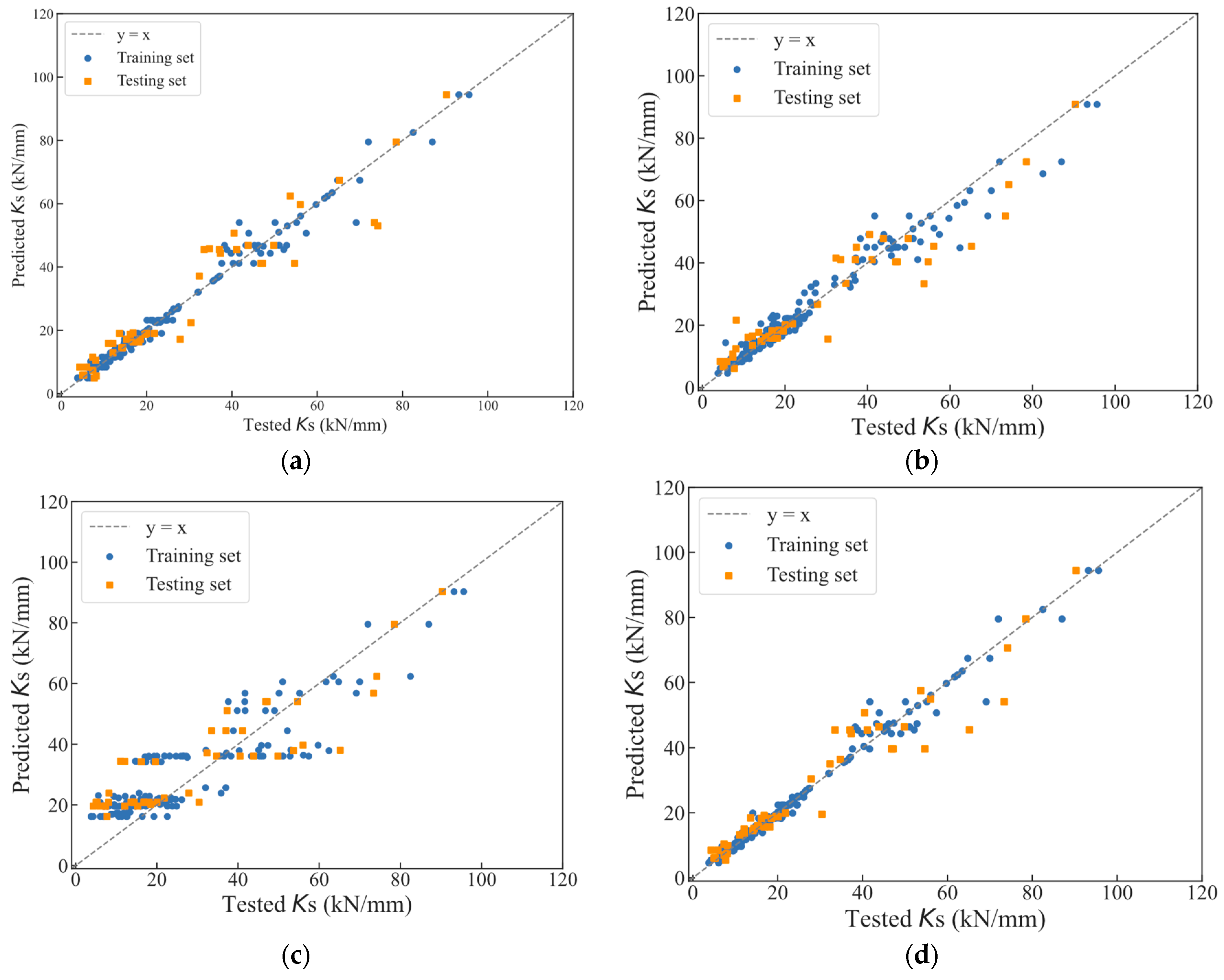
Figure 8 shows comparisons between the experimental values and the prediction results for all the adopted ML models. By means of simple random sampling, the samples in the data set are divided into the training set (80%) and the testing set (20%). To compare the prediction accuracies of the models, Table 2 lists the performance of the ML models evaluated using different quantitative indices. Figure 8 and Table 2 demonstrate that the four adopted ML models can accurately predict the slip modulus of the TCC screwed connection, with R2 values larger than 0.80. This indicates that the ML models achieve good prediction performance.
As shown in Table 2, the scores of the four indices of the GBRT algorithm on the training and testing data sets are the best among the compared models. The GBRT algorithm achieves an R2 value of 0.9197 on the testing data set, indicating excellent prediction performance for the slip modulus of TCC screwed connections. In terms of MAE, RMSE, and MAPE, the GBRT algorithm also exhibits the best prediction accuracy with the lowest values of these associated indices. Moreover, a high fitting accuracy can explain the changes in the target variables in the testing data set well, which is valuable when push-out testing results exhibit high variations. Owing to the best prediction accuracy, the prediction result based on the GBRT model is discussed below.

4.3. Interpretation of the GBRT Model Using Shapley Additive Explanations

Shapley Additive Explanations (SHAP), proposed by Lundberg and Lee [78], are an advanced method for explaining ML model prediction results. The SHAP method can effectively assess the effects of the input features on prediction results. Hence, SHAP has been widely used in previous investigations [68,76].
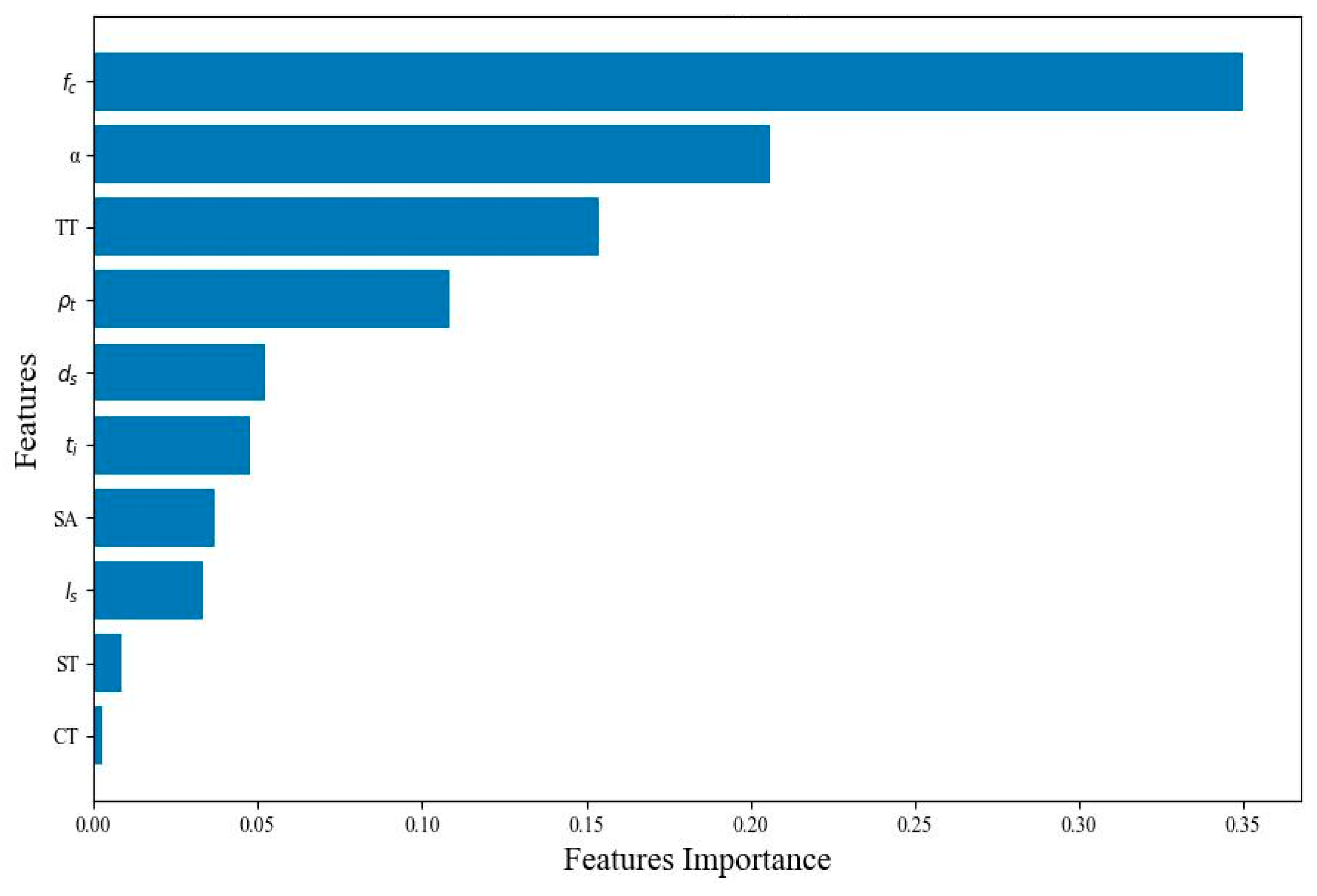
Figure 9 shows the SHAP values of all input features, ordered from the largest to the smallest value. The concrete compressive strength, fc, exerts the greatest influence on the slip modulus of TCC screwed connections, followed by the screw inclination angle, α, the timber type, and the timber density, ρt. Moreover, the screw diameter, ds, the interlayer thickness, ti, the screw arrangement method, and the screw penetration depth, ls, show similar influences on the slip modulus of screwed connections. The effect of the screw type and the concrete type on the connection slip modulus can be ignored. The SHAP values are in exact agreement with the experimental results. For example, the experimental results revealed that, with an increase in the concrete strength and grade, the slip modulus of the screwed connection was improved [26,54]. Similarly, for the screw inclination angle, α, the connection with shear–tension screws, which possess a smaller inclination angle, was demonstrated to achieve better connection performance [21,51].
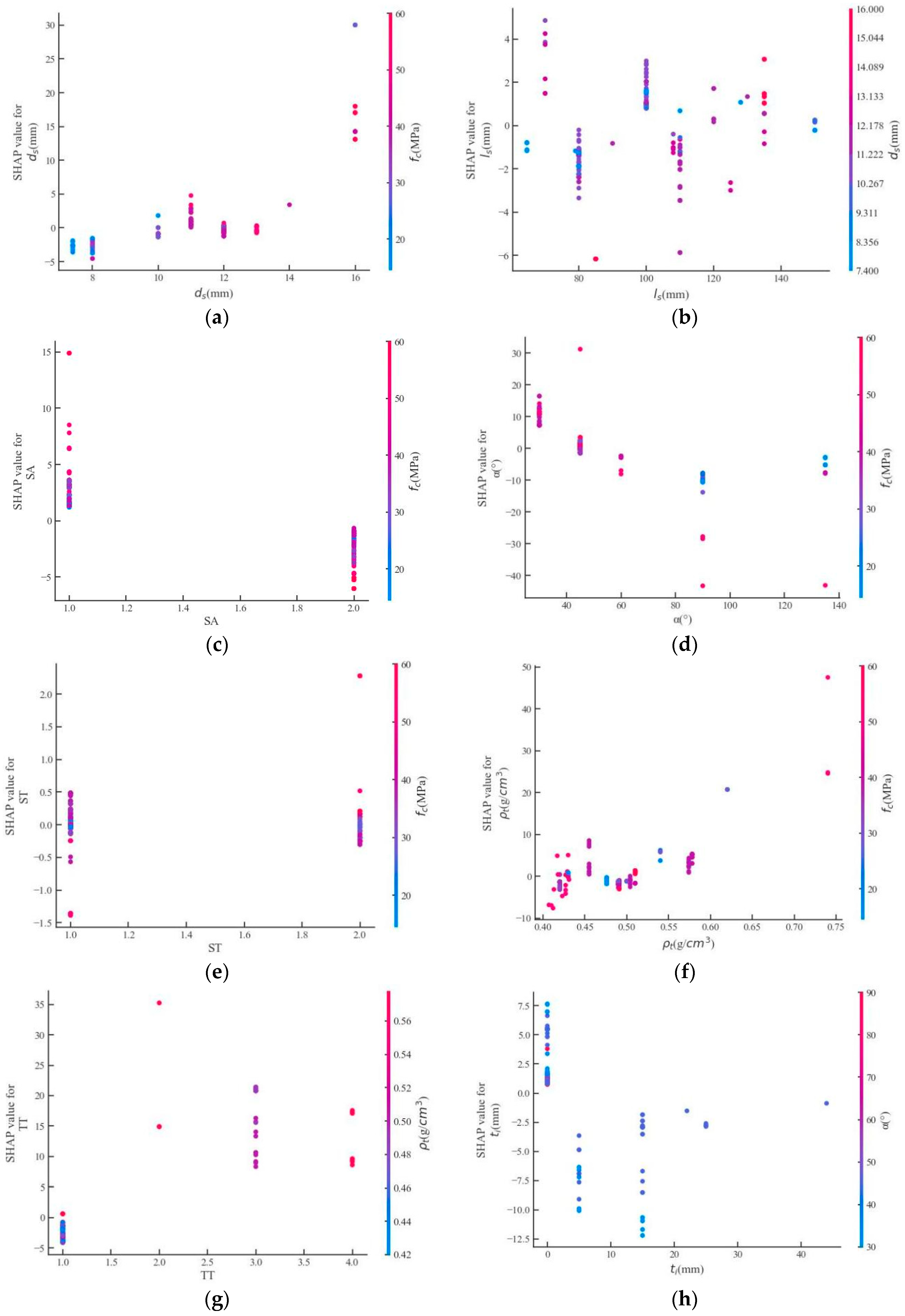
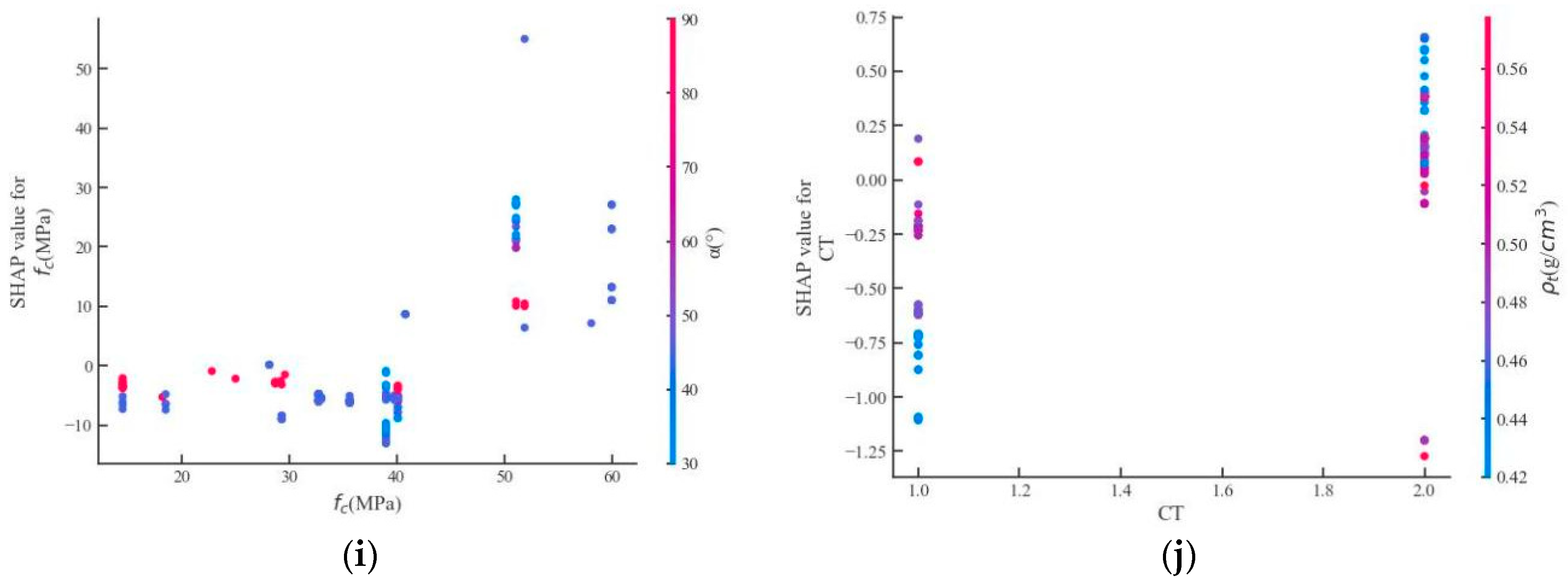
Figure 10 also shows the influence of all input features on the slip modulus of the screw connections. It can be concluded that the feature values of the screw diameter (ds), the timber density (ρt), and the concrete compressive strength (fc) have a positive effect on the slip modulus of TCC screwed connections, as shown in Figure 10a,f,i. For example, the SHAP value has a significant increase when the concrete compressive strength (fc) is larger than 40 MPa. By contrast, with an increase in the screw inclination angle, the slip modulus of the screwed connections decreases, as shown in Figure 10d. Similarly, the interlayer thickness (ti) also has a negative effect on the slip modulus of the TCC screwed connections, as shown in Figure 10h, and lower ti values result in a higher slip modulus.
However, the screw penetration depth (ls) had no regular effect on the slip modulus of the screwed connection, as shown in Figure 10b. This is because a sufficient penetration depth is required in the connection system design process. Regarding to screw arrangement methods, the unidirectional screw connection (eigenvalue 1) showed an approximately higher slip modulus than the bidirectional screw connection (eigenvalue 2), as shown in Figure 10c, owing to the contribution of the higher slip modulus of shear–tension screw for a screw inclination angle smaller than 90°. Figure 10e reveals that the connection using a hexagonal head screw (eigenvalue 2) basically shows similar SHAP values to those using a self-tapping screw (eigenvalue1). As shown in Figure 10j, adopting NC instead of LWAC obviously improves the slip modulus of the screwed connection.
In order to visually observe the influence of the features on the slip modulus, this paper selects several significant features from the data set and lists comparative cases under the same study conditions. The examples are listed in Table 3, in which the line number denotes the positions of the data in the data set uploaded in GitHub (https://github.com/Lww-creator/Timber-Concrete-ML, accessed on 25 June 2025). It can be found that the trend of the influence of the features reflected in the testing results is consistent with the results of the SHAP analysis.

4.4. Interpretation of GBRT

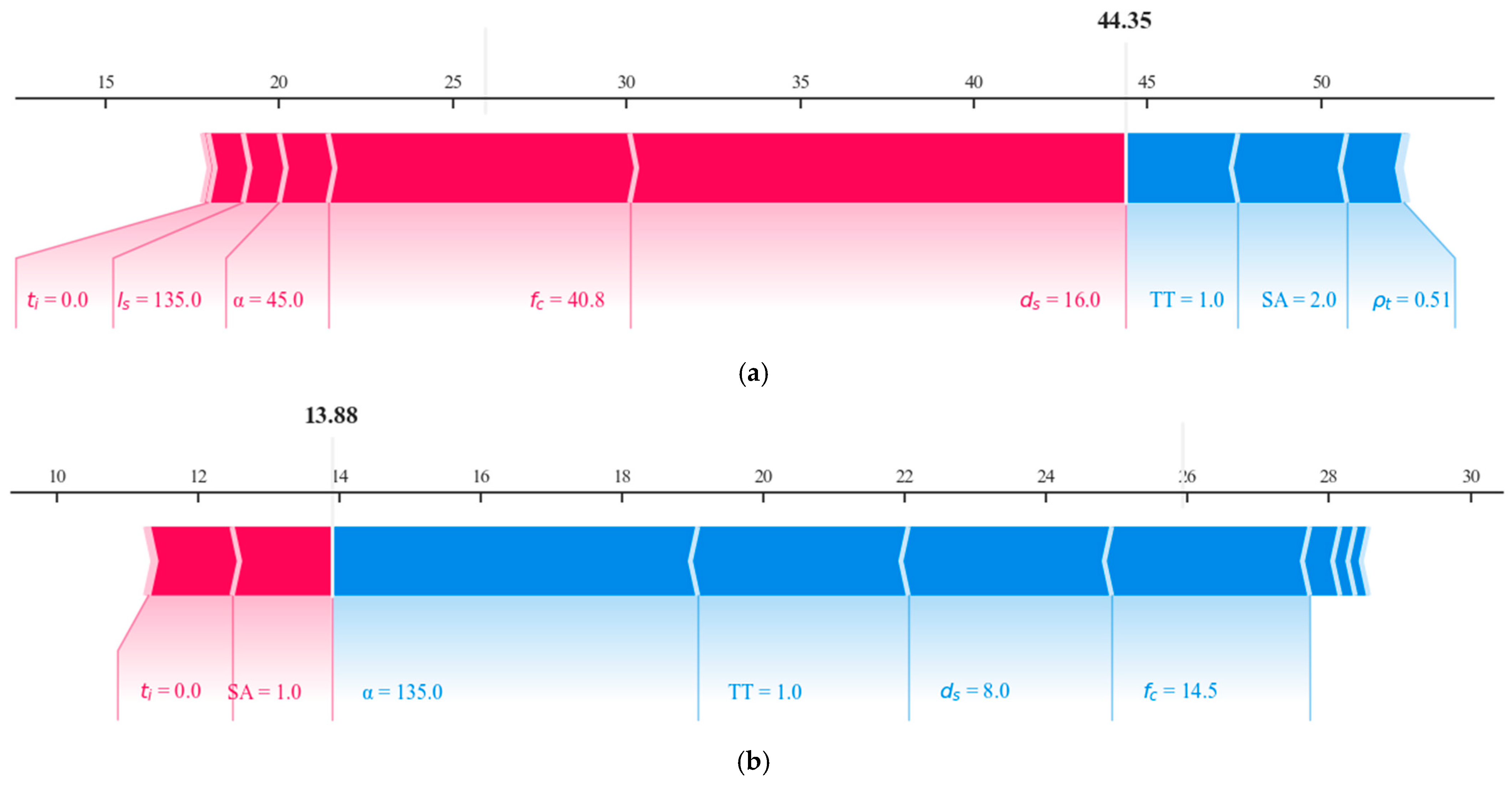
Two typical experimental cases reported by Tao et al. [26] (specimen CBIS16-200-4) and Appavuravther et al. [22] (specimen S-M8-200-45-B) are shown in Figure 11. The dataset sample numbers of specimens CBIS16-200-4 and S-M8-200-45-B are No. 43 and No. 58, respectively. The eigenvalues of testing data samples No. 43 and No. 58 in the SA feature are 2 and 1, respectively. The red area in Figure 11 indicates that the parameters have a positive impact on the interfacial slip modulus, whereas the blue area indicates that the parameters have a negative impact.
As shown in Figure 11a, the predicted slip modulus of specimen CBIS16-2003-4 is 44.35 kN/mm. Comparatively, its experimental value is 41.75 kN/mm, and the average slip modulus of the group to which it belongs was 42.92 kN/mm. Thus, the GBRT model demonstrates good prediction accuracy. Moreover, the large diameter, the absence of an interlayer, the high concrete compressive strength, and the small screw inclination angle resulted in a specimen with a relatively high slip modulus.
As shown in Figure 11b, the predicted value for the slip modulus of specimen S-M8-200-45-B is 13.88 kN/mm, and the corresponding experimental value is 13.040 kN/mm. The large screw inclination angle (135°), the relatively small screw diameter, and the low concrete compressive strength result in a relatively low slip modulus compared to that of specimen CBIS16-2003-4.

5. Compared with Existing Models

5.1. Existing Analytical Methods

In Section 4, the accuracy of the ML models is verified through four quantitative indices and two actual case studies, and it is demonstrated that the GBRT algorithm achieves the best prediction result among the models adopted. To further demonstrate the accuracy and wider applicability of the ML models, the GBRT algorithm is selected for comparison with existing analytical methods.
(a)
Empirical formula suggested in Eurocode 5 [29].
Eurocode 5 introduces the lateral slip stiffness of the screwed connectors in timber structures, as shown in Equation (10). The formula should be multiplied by 2 when it is used to predict the slip modulus of vertical and shear–compression screw connections in TCC structures [18,26,51].
K s = ρ t 1.5 d s 23
(b)
Dias’s model [79].
Based on the theory of the elastic foundation beam model, Dias [79] established a theoretical model for a vertical screw connection, in which one-element and two-element models were separately established by assuming that the concrete foundation modulus is elastic or rigid. Considering that concrete can provide sufficient constraint for screws and the concrete foundation modulus is relatively difficult to determine, the one-element theoretical model is selected to predict the slip modulus of a TCC screwed connection, as follows:
K s = 4 E s I s λ 3
where Es denotes the elastic modulus of the metal screws, and it is determined to be 210 GPa according to Eurocode 3 [80], Is represents the inertia moment of the screw (mm4), λ = k t / ( 4 E s I s ) 1 / 4 , and kt denotes the linear foundation modulus of the timber (N/mm2).
(c)
Wilkinson’s model [81].
Wilkinson [81] proposed a semi-empirical calculation method. In this model, the interface slip modulus was affected by the elastic modulus of the screw, the timber foundation modulus, and the screw diameter, as shown in Equation (12).
K s = 1 6 E s 1 4 k t 3 4 d s 7 4
(d)
Theoretical formula proposed by Du et al. [51].
Du et al. [51] established a formula for a unidirectional inclined screw connection when the screw inclination angle is less than 90°, i.e., a shear–tension screw connection, by considering the contribution of the pulling-out stiffness of the inclined screws. This concept was initially proposed by Marchi et al. [18]. The interface slip modulus of the shear–tension screw connection can be calculated via Equation (13).
K s = K sin α 2 + K / / cos α 2
where K denotes the slip modulus component provided by the embedment stiffness of timber, which can be calculated by Equation (10); K / / denotes the slip modulus component provided via the pull-out stiffness of the screw, which can be calculated by Equation (14).
K / / = 234 ( d s ρ t ) 0.2 l s 0.4
where ls denotes the effective penetration length of the screw drilled into the timber.
(e)
Theoretical formula proposed by Tao et al. [26]
Tao et al. [26] established a theoretical calculation method for the slip modulus of a bidirectional inclined screw connection by superposing the slip modulus provided via the shear–tension and shear–compression screws, as shown in Equation (15). For the shear–tension screw, the slip modulus calculation method was derived according to the elastic foundation beam theory. For the shear–compression screw, the slip modulus calculation method adopted the work of Stamatopoulos and Malo [82].
K s = K s 1 + K s 2
where Ks1 and Ks2 are slip modulus components provided via shear–tension and shear–compression screws, respectively. Ks1 conforms to the idea of Equation (13), in which K and K / / are calculated by Equation (16) and Equations (17)–(19), respectively. Ks2 is calculated via Equation (10).
K = k t ( sin 2 λ l s + sinh 2 λ l s ) λ sin α ( cos 2 λ l s + cosh 2 λ l s + 2 )
K / / = w E s A s l s tanh w
w = 2 k ax E s d s l s
k ax = 9.35 1.5 sin 2.2 α + cos 2.2 α
where As denotes the cross-sectional area of the screw, kax indicates the pull-out modulus of the screw pulled out of the timber, which is an empirical regression formula adopted by Stamatopoulos and Malo [82], and w is a stiffness factor considering the effects of metal fasteners.
To calculate Equations (11), (12), and (16), the timber foundation modulus, kt, must be determined. To uniformly determine the linear modulus of kt, the empirical regression formula proposed by Mirdad et al. [83] was adopted, as shown in Equation (20).
k t = 0.00011 ρ t 2.443 d s 0.044 7.663 cos 2 α + 2.645 sin 2 α

5.2. Accuracy of Existing Design Methods

Table 4 presents the results of the four evaluation indices for the five design models and two typical ML methods for the prediction of the connection with a pair of screw. GBRT and AdaBoost exhibit the highest and lowest prediction accuracies, respectively, in accordance with Table 2 among the adopted four ML methods. The prediction results of the five design models are calculated via Equations (10)–(20), respectively.
The formula given in Eurocode 5 [29] was used to predict the slip modulus of a vertical screw connection. However, the R2 value of the formula in Eurocode 5 is still lower than that of the AdaBoost algorithm used in the prediction of the whole testing set. Moreover, the prediction accuracy of the four other design methods, which are suitable for different specific arrangements, is lower than that of the formula (Equation (10)) in Eurocode 5. In addition, two of them show negative R2 values, which denote the relatively poor prediction accuracy. The values of RMSE, MAE, and MAPE also indicate that the existing design methods cannot accurately capture the real change trend and distribution characteristics of the corresponding data set.
Moreover, the aforementioned design methods face certain limitations. For example, they only apply to specific forms of connection arrangements, and most of the aforementioned design methods cannot be used to predict the screwed connections with an interlayer. In addition, for the theoretical calculation methods, the determination of kt and kax based on the empirical equation may affect the prediction accuracy because of various tree species, screw dimensions, and penetration depths.
By comparing the prediction results of the ML-based algorithms (Table 2, Figure 8, Figure 9 and Figure 10) and the design methods (Table 4), it can be concluded that the ML methods achieve significant advantages concerning the following aspects:
(i)
High accuracy and extensive applicability. The ML-based methods show better prediction accuracy in terms of the four quantitative indices. In addition, the existing theoretical and empirical models mostly apply to a specific connection arrangement depicted in Figure 2. ML-based methods can be used for the slip modulus prediction of any potential connection arrangement, as well as connection-dimensional parameters and material characteristics, which are covered in the data set.
(ii)
Discovery in the interface slip mechanism of a TCC screwed connection. With the use of the SHAP framework, the importance of each feature and its influence on the slip modulus of screwed connections are shown in Figure 9 and Figure 10, respectively. This provides guidance for the optimal design of TCC screwed connections. Particularly, the compressive strength, which is largely overlooked in existing design models, has been verified to exert significantly positive effects on the slip modulus, whereas the influence of the interlayer thickness may have been overestimated in the past [52].
(iii)
High feasibility and convenience. The physical characteristics (input features) of the screwed connection covered in the data set are easy to obtain and determine, which means that the prediction using ML-based methods is remarkably convenient in the process of service engineering design. For comparison, the theoretical and empirical models rely on the determination of the timber foundation coefficient, axial screw pull-out modulus, and concrete foundation coefficient that need to be determined through material tests.

6. Conclusions

This study made a new attempt to introduce the ML method to predicting the slip modulus of a TCC screwed connection. Four ML methods (DT, RF, AdaBoost, and GBRT) were adopted to establish the prediction algorithm, and the SHAP framework was adopted to interpret the ML model prediction results and reveal the slip mechanism of the TCC screwed connection. A total of 222 sets of experimental data from 17 studies were collected to establish the data set, and they were randomly divided into training and testing sets. The prediction accuracies of the four ML methods and five analytical methods were compared using four quantitative indices. The main conclusions are summarized as follows:
(i)
GBRT shows the highest accuracy in terms of R2, RMSE, MAE, and MAPE compared with the other three ML algorithms. The GBRT algorithm for the training and testing sets showed R2 values of 0.9879 and 0.9197, respectively, followed by the DT algorithm corresponding to R2 values of 0.9872 and 0.9076, respectively.
(ii)
The ML algorithms demonstrate higher prediction accuracy and applicability than existing design methods. The empirical formula listed in Eurocode 5 exhibits acceptable accuracy only when it is applied to predict the slip modulus of vertical screw connections without interlayers. The theoretical models face limitations in the arrangement of screws, the presence of an interlayer, and the determination of some physical parameters.
(iii)
Through the SHAP framework, it was verified that the concrete compressive strength exerts the highest influence on the slip modulus of the TCC screwed connection, which is overlooked in existing theoretical models. The SHAP values of the screw inclination, the timber type, and the density, which also greatly affect the slip modulus, follow closely behind the concrete compressive strength.
(iv)
Through an input feature impact analysis and two typical experimental cases, it was demonstrated that increasing the timber density, concrete compressive strength, and screw diameter, as well as decreasing the screw inclination angle and interlayer thickness, can effectively improve the slip modulus of TCC screwed connections, which can provide diverse choices for the performance-based design of TCC structures. The machine-learning method tested in this study can be effectively applied to predict the slip modulus of the screwed connections, providing precise predictions for the parametric and performance-based design of interface connections in timber–concrete composite structures.
The present study can provide a reference for the design of TCC structures with screwed connections. The code of the four models adopted in this study, as well as the collected database of the screwed connections, is available via GitHub (https://github.com/Lww-creator/Timber-Concrete-ML, accessed on 25 June 2025). This article only employed four common machine-learning methods. In the next step, more advanced ensemble machine-learning methods will be adopted. Further work will focus on the development of ML methods to predict the shear performances of other TCC shear connections, such as the notched-screw and glued-in steel-plate ones.

Author Contributions

Conceptualization, H.-F.Y. and B.-K.S.; Methodology, J.-G.X. and B.-K.S.; Software, W.-W.L.; Validation, Y.-W.C., J.-G.X., H.-F.Y., H.-T.T. and W.Z.; Formal analysis, W.-W.L. and J.-G.X.; Investigation, W.-W.L.; Resources, H.-F.Y.; Data curation, Y.-W.C. and H.-T.T.; Writing—original draft, W.-W.L.; Writing—review & editing, Y.-W.C., H.-F.Y., H.-T.T., W.Z. and B.-K.S.; Project administration, B.-K.S. All authors have read and agreed to the published version of the manuscript.

Funding

The authors of this study highly appreciate the support provided by the National Natural Science Foundation of China (Grant No. 52208253, 52308173, and 51878344).

Data Availability Statement

Data will be made available on request.

Conflicts of Interest

The authors declare no conflicts of interest.

References

  1. Dias, A.; Skinner, J.; Crews, K.; Tannert, T. Timber-concrete-composites increasing the use of timber in construction. Eur. J. Wood Prod. 2016, 74, 443–451. [Google Scholar] [CrossRef]
  2. Frangi, A.; Knobloch, M.; Fontana, M. Fire design of timber-concrete composite slabs with screwed connections. J. Struct. Eng. 2010, 136, 219–228. [Google Scholar] [CrossRef]
  3. Wen, B.; Tao, H.; Shi, B.; Yang, H. Dynamic properties of timber–concrete composite beams with crossed inclined coach screw connections: Experimental and theoretical investigations. Buildings 2023, 13, 2268. [Google Scholar] [CrossRef]
  4. Zhang, C.; Lu, X.; Shi, B.; Yang, H.; Tao, H.; Liu, J. Experimental and numerical investigations on flexural behavior of stress-laminated timber-concrete composite decks with butt joints. Eng. Struct. 2024, 316, 118534. [Google Scholar] [CrossRef]
  5. Höltke, T.; Bleicher, A. Experimental and numerical investigations of a timber-concrete composite frame joint for high-rise buildings. Eng. Struct. 2025, 333, 120034. [Google Scholar] [CrossRef]
  6. Otero-Chans, D.; Suárez-Riestra, F.; Martín-Gutiérrez, E.; Estévez-Cimadevila, J. Experimental and numerical analysis of a full-scale timber-concrete-composite beam from simply supported to frame-connected. Eng. Struct. 2025, 327, 119624. [Google Scholar] [CrossRef]
  7. Chen, H.; Ma, W.; Kasal, B.; Wei, Y.; Yan, L. Flexural behavior of adhesively bonded cross-laminated timber-concrete composite (TCC) panel with glass-fiber textile mesh as reinforcement in concrete: Experimental studying and numerical simulation. Eng. Struct. 2025, 330, 119916. [Google Scholar] [CrossRef]
  8. Tao, H.; Yang, H.; Zhou, Z.; Wu, Y.; Ju, G.; Shi, B. Influence of slab composite effect on the seismic performance of a six-story timber-concrete composite moment-resisting frame. J. Build. Eng. 2025, 101, 111815. [Google Scholar] [CrossRef]
  9. Shi, B.; Zhou, X.; Tao, H.; Yang, H.; Wen, B. Long-term behavior of timber–concrete composite structures: A literature review on experimental and numerical investigations. Buildings 2024, 14, 1770. [Google Scholar] [CrossRef]
  10. Yang, H.; Lu, Y.; Ling, X.; Tao, H.; Shi, B. Experimental and theoretical investigation on shear performances of glued-in perforated steel plate connections for prefabricated timber–concrete composite beams. Case Stud. Constr. Mater. 2023, 18, e01885. [Google Scholar] [CrossRef]
  11. Rasmussen, P.K.; Sørensen, J.H.; Hoang, L.C.; Feddersen, B.; Larsen, F. Notched connection in timber-concrete composite deck structures: A literature review on push-off experiments & design approaches. Constr. Build. Mater. 2023, 397, 131761. [Google Scholar] [CrossRef]
  12. Shi, B.; Dai, Y.; Tao, H.; Yang, H. Shear performances of hybrid notch-screw connections for timber-concrete composite structures. BioResources 2022, 17, 2259–2274. [Google Scholar] [CrossRef]
  13. Zhang, L.; Zhou, J.; Chui, Y.H. Development of high-performance timber-concrete composite floors with reinforced notched connections. Structures 2022, 39, 945–957. [Google Scholar] [CrossRef]
  14. Suárez-Riestra, F.; Estévez-Cimadevila, J.; Martín-Gutierrez, E.; Otero-Chans, D. Perforated shear + reinforcement bar connectors in a timber-concrete composite solution. Analytical and numerical approach. Compos. Part B Eng. 2019, 156, 138–147. [Google Scholar] [CrossRef]
  15. Dias, A.; Schaenzlin, J.; Dietsch, P. Design of Timber-Concrete Composite Structures, COST Action FP1402/WG4; Shaker Verlag: Düren, Germany, 2018. [Google Scholar]
  16. Steinberg, E.; Selle, R.; Faust, T. Connectors for timber–lightweight concrete composite structures. J. Struct. Eng. 2013, 129, 1538–1545. [Google Scholar] [CrossRef]
  17. Dias, A.M.P.G.; Cruz, H.M.P.; Lopes, S.M.R.; van de Kuilen, J.W. Stiffness of dowel-type fasteners in timber–concrete joints. Proc. Inst. Civ. Eng. -Struct. Build. 2010, 163, 257–266. [Google Scholar] [CrossRef]
  18. Marchi, L.; Scotta, R.; Pozza, L. Experimental and theoretical evaluation of TCC connections with inclined self-tapping screws. Mater. Struct. 2017, 50, 180. [Google Scholar] [CrossRef]
  19. Symons, D.; Persaud, R.; Stanislaus, H. Slip modulus of inclined screws in timber–concrete floors. Proc. Inst. Civ. Eng. -Struct. Build. 2010, 163, 245–255. [Google Scholar] [CrossRef]
  20. Gan, Z.; Sun, Y.; Sun, X. Push-out performance of inclined screw shear connectors used in nail-laminated timber-concrete composite. Constr. Build. Mater. 2023, 366, 130175. [Google Scholar] [CrossRef]
  21. Sebastian, W.; Piazza, M.; Harvey, T.; Webster, T. Forward and Reverse shear transfer in beech LVL-concrete composites with singly inclined coach screw connectors. Eng. Struct. 2018, 175, 231–244. [Google Scholar] [CrossRef]
  22. Appavuravther, E.; Vandoren, B.; Henriques, J. Behaviour of screw connections in timber-concrete composites using low strength lightweight concrete. Constr. Build. Mater. 2021, 28, 122973. [Google Scholar] [CrossRef]
  23. Martins, C.; Dias, A.M.; Costa, R.; Santos, P. Environmentally friendly high performance timber–concrete panel. Constr. Build. Mater. 2016, 102, 1060–1069. [Google Scholar] [CrossRef]
  24. Tao, H.; Yang, H.; Ju, G.; Xu, J.; Shi, B. Effective width of timber-concrete composite beams with crossed inclined coach screw connections at the serviceability state. Eng. Struct. 2022, 267, 114716. [Google Scholar] [CrossRef]
  25. Zhu, W.; Yang, H.; Liu, W.; Shi, B.; Ling, Z.; Tao, H. Experimental investigation on innovative connections for timber–concrete composite systems. Constr. Build. Mater. 2019, 207, 345–356. [Google Scholar] [CrossRef]
  26. Tao, H.T.; Yang, H.F.; Liu, W.Q.; Wang, C.; Shi, B.; Ling, X. Mechanical behavior of crossed inclined coach screw shear connections for prefabricated timber-concrete composite structures. J. Build. Struct. 2022, 43, 164–174. (In Chinese) [Google Scholar] [CrossRef]
  27. Deam, B.L.; Fragiacomo, M.; Buchanan, A.H. Connections for composite concrete slab and LVL flooring systems. Mater. Struct. 2008, 41, 495–507. [Google Scholar] [CrossRef]
  28. China Association for Engineering Construction Standardization. Technical Standard for Timber-Concrete Composite Structures; China Architecture & Building Press: Beijing, China, impending publication.
  29. EN 1995-1-1:2004; Eurocode 5: Design of Timber Structures—Part 1–1: General—Common Rules and Rules for Buildings. European Committee for Standardization: Brussels, Belgium, 2004.
  30. Auclair, S.C. Design Guide for Timber-Concrete Composite Floors in Canada; FPInnovations: Pointe-Claire, QC, Canada, 2020. [Google Scholar]
  31. Di Nino, S.; Gregori, A.; Fragiacomo, M. Experimental and numerical investigations on timber-concrete connections with inclined screws. Eng. Struct. 2020, 209, 109993. [Google Scholar] [CrossRef]
  32. Mirdad, A.H.; Chui, Y.H. Stiffness prediction of Mass Timber Panel-Concrete (MTPC) composite connection with inclined screws and a gap. Eng. Struct. 2020, 207, 110215. [Google Scholar] [CrossRef]
  33. Chou, J.-S.; Tsai, C.-F.; Pham, A.-D.; Lu, Y.-H. Machine learning in concrete strength simulations: Multi-nation data analytics. Constr. Build. Mater. 2014, 73, 771–780. [Google Scholar] [CrossRef]
  34. Sun, H.; Burton, H.V.; Huang, H. Machine learning applications for building structural design and performance assessment: State-of-the-art review. J. Build. Eng. 2021, 33, 101816. [Google Scholar] [CrossRef]
  35. Xu, J.-G.; Hong, W.; Zhang, J.; Hou, S.-T.; Wu, G. Seismic performance assessment of corroded RC columns based on data-driven machine-learning approach. Eng. Struct. 2022, 255, 113936. [Google Scholar] [CrossRef]
  36. Zhang, S.; Xu, J.; Lai, T.; Yu, Y.; Xiong, W. Bond stress estimation of profiled steel-concrete in steel reinforced concrete composite structures using ensemble machine learning approaches. Eng. Struct. 2023, 294, 116725. [Google Scholar] [CrossRef]
  37. Kazemi, F.; Asgarkhani, N.; Jankowski, R. Optimization-based stacked machine-learning method for seismic probability and risk assessment of reinforced concrete shear walls. Expert Syst. Appl. 2024, 255, 124897. [Google Scholar] [CrossRef]
  38. van Blokland, J.; Nasir, V.; Cool, J.; Avramidis, S.; Adamopoulos, S. Machine learning-based prediction of surface checks and bending properties in weathered thermally modified timber. Constr. Build. Mater. 2021, 307, 124996. [Google Scholar] [CrossRef]
  39. Li, Z.; Tao, D.; Li, M. Prediction of damage accumulation effect of wood structural members under long-term service: A machine learning approach. Materials 2019, 12, 1243. [Google Scholar] [CrossRef]
  40. Shams, S.A.; Ge, H.; Wang, L. Hygrothermal modeling in mass timber constructions: Recent advances and machine learning prospects. J. Build. Eng. 2024, 96, 110500. [Google Scholar] [CrossRef]
  41. Rahimi, S.; Avramidis, S.; Sassani, F.; Nasir, V. Machine learning-based prediction of internal moisture variation in kiln-dried timber, Wood Mater. Sci. Eng. 2024, 19, 499–510. [Google Scholar] [CrossRef]
  42. EN 26891:1991; Timber Structures—Joints Made with Mechanical Fasteners—General Principles for the Determination of Strength and Deformation Characteristics. European Committee for Standardization: Brussels, Belgium, 1991.
  43. Ling, Z.B.; Li, Z.-J.; Rong, X.Q. Effect of test configurations and loading protocols on performance of timber-concrete connectors. Constr. Build. Mater. 2023, 367, 130244. [Google Scholar] [CrossRef]
  44. Mirdad, M.A.H.; Chui, Y.H. Load-slip performance of Mass Timber Panel-Concrete (MTPC) composite connection with Self-tapping screws and insulation layer. Constr. Build. Mater. 2019, 213, 696–708. [Google Scholar] [CrossRef]
  45. Berardinucci, B.; Di Nino, S.; Gregori, A.; Fragiacomo, M. Mechanical behavior of timber–concrete connections with inclined screws. Int. J. Comp. Meth. Exp. Meas. 2017, 5, 807–820. [Google Scholar] [CrossRef]
  46. Jiang, Y.-C. Mechanical Behaviour and Design Methods of Glulam-Lightweight Concrete Composite Beams. Ph.D. Thesis, Nanjing Tech University, Nanjing, China, 2018. (In Chinese). [Google Scholar]
  47. Huang, B.-W. Investigations on Flexural Behavior of Timber-Lightweight Concrete Composite Beams. Master’s Thesis, Nanjing Tech University, Nanjing, China, 2022. (In Chinese). [Google Scholar]
  48. Bao, Y.-W. Study on Flexural Behavior of Cross Laminated Timber (CLT)–Concrete Composite Floor. Master’s Thesis, Nanjing Tech University, Nanjing, China, 2021. (In Chinese). [Google Scholar]
  49. Du, H.; Hu, X.; Sun, Z.; Meng, Y.; Han, G. Load carrying capacity of inclined crossing screws in glulam-concrete composite beam with an interlayer. Compos. Struct. 2020, 245, 112333. [Google Scholar] [CrossRef]
  50. Du, H.; Hu, X.-M.; Wang, H.-C.; Zhang, J.; Sun, Z.-X. Shear performance of inclined screws in glulam-concrete composite beams. J. Build. Struct. 2020, 41, 191–200. (In Chinese) [Google Scholar]
  51. Du, H.; Hu, X.; Xie, Z.; Wang, H. Study on shear behavior of inclined cross lag screws for glulam-concrete composite beams. Constr. Build. Mater. 2019, 224, 132–143. [Google Scholar] [CrossRef]
  52. Jorge, L.F.C.; Lopes, S.M.R.; Cruz, H.M.P. Interlayer Influence on Timber-LWAC Composite Structures with Screw Connections. J. Struct. Eng. 2011, 137, 618–624. [Google Scholar] [CrossRef]
  53. Bao, Y.; Lu, W.; Yue, K.; Zhou, H.; Lu, B.; Chen, Z. Structural performance of cross-laminated timber-concrete composite floors with inclined self-tapping screws bearing unidirectional tension-shear loads. J. Build. Eng. 2022, 55, 104653. [Google Scholar] [CrossRef]
  54. Jiang, Y.; Hong, W.; Hu, X.; Crocetti, R.; Wang, L.; Sun, W. Early-age performance of lag screw shear connections for glulam-lightweight concrete composite beams. Constr. Build. Mater. 2017, 151, 36–42. [Google Scholar] [CrossRef]
  55. Derikvand, M.; Fink, G. Deconstructable connector for TCC floors using self-tapping screws. J. Build. Eng. 2021, 42, 102495. [Google Scholar] [CrossRef]
  56. Du, H.; Xu, R.; Liu, P.; Yuan, S.; Wei, Y. Experimental and theoretical evaluation of inclined screws in glued laminated bamboo and timber-concrete composite beams. J. Build. Eng. 2024, 91, 109579. [Google Scholar] [CrossRef]
  57. Tao, H.; Yang, H.; Liu, W.; Wang, C.; Shi, B.; Ling, X. Experimental and nonlinear analytical studies on prefabricated timber–concrete composite structures with crossed inclined coach screw connections. J. Struct. Eng. 2021, 147, 04021043. [Google Scholar] [CrossRef]
  58. Niederwestberg, J.; Zhou, J.; Chui, Y.-H. Mechanical properties of innovative, multi-layer composite laminated panels. Buildings 2018, 8, 142. [Google Scholar] [CrossRef]
  59. Chen, D.; Montano, V.; Huo, L.; Song, G. Depth detection of subsurface voids in concrete-filled steel tubular (CFST) structure using percussion and decision tree. Measurement 2020, 163, 107869. [Google Scholar] [CrossRef]
  60. Zhang, S.; Chen, X.; Ran, X.; Li, Z.; Cao, W. Prioritizing causation in decision trees: A gramework for interpretable modeling. Eng. Appl. Artif. Intel. 2024, 133 Pt C, 108224. [Google Scholar] [CrossRef]
  61. He, Z.; Wang, J.; Jiang, M.; Hu, L.; Zou, Q. Random subsequence forests. Inform. Sci. 2024, 667, 120478. [Google Scholar] [CrossRef]
  62. Bhatt, P.P.; Sharma, N.; Kodur, V.K.R.; Naser, M.Z. Machine learning approach for predicting fire resistance of FRP-strengthened concrete beams. Struct. Concr. 2024, 1–23. [Google Scholar] [CrossRef]
  63. Arasteh-Khoshbin, O.; Seyedpour, S.M.; Mandl, L.; Lambers, L.; Ricken, T. Comparing durability and compressive strength predictions of hyperoptimized random forests and artificial neural networks on a small dataset of concrete containing nano SiO2 and RHA. Eur. J. Environ. Civ. Eng. 2024, 1–20. [Google Scholar] [CrossRef]
  64. Kim, T.-K.; Hwang, S.-H.; Kim, J.; Jung, W.-T.; Yoon, J. Analysis of bond strength of CFRP cables with concrete using random forest model. J. Build. Eng. 2024, 96, 110658. [Google Scholar] [CrossRef]
  65. Li, R.-H.; Li, M.-Y.; Zhu, X.-Y.; Zeng, X.-W. Application of random forest algorithm in estimating dynamic mechanical behaviors of reinforced concrete column members. Appl. Sci. 2024, 14, 2546. [Google Scholar] [CrossRef]
  66. Lei, Q.; Yu, H.; Lin, Z. Understanding China’s CO2 emission drivers: Insights from random forest analysis and remote sensing data. Heliyon 2024, 10, e29086. [Google Scholar] [CrossRef]
  67. Cai, R.; Han, T.; Liao, W.; Huang, J.; Li, D.; Kumar, A.; Ma, H. Prediction of surface chloride concentration of marine concrete using ensemble machine learning. Cem. Concr. Res. 2020, 136, 106164. [Google Scholar] [CrossRef]
  68. Feng, J.; Zhang, H.; Gao, K.; Liao, Y.; Yang, J.; Wu, G. A machine learning and game theory-based approach for predicting creep behavior of recycled aggregate concrete. Case Stud. Constr. Mater. 2022, 17, e01653. [Google Scholar] [CrossRef]
  69. Chao, Z.; Li, Z.; Dong, Y.; Shi, D.; Zheng, J. Estimating compressive strength of coral sand aggregate concrete in marine environment by combining physical experiments and machine learning-based techniques. Ocean Eng. 2024, 308, 118320. [Google Scholar] [CrossRef]
  70. Jiang, J.; Xin, C.; Wu, S.; Chen, W.; Li, H.; Ran, Z.; Rao, K.R. Enhancing concrete workability prediction through ensemble learning models: Emphasis on slump and material factors. Adv. Civ. Eng. 2024, 2024, 4616609. [Google Scholar] [CrossRef]
  71. Wudil, Y.S.; Al-Fakih, A.; Al-Osta, M.A.; Gondal, M. Effective carbon footprint assessment strategy in fly ash geopolymer concrete based on adaptive boosting learning techniques. Environ. Res. 2025, 266, 120570. [Google Scholar] [CrossRef]
  72. Friedman, J.H. Greedy function approximation: A gradient boosting machine. Ann. Stat. 2001, 29, 1189–1232. [Google Scholar] [CrossRef]
  73. Xu, N.; Wang, Z.; Dai, Y.; Li, Q.; Zhu, W.; Wang, R.; Finkelman, R.B. Prediction of higher heating value of coal based on gradient boosting regression tree model. Int. J. Coal Geol. 2023, 274, 104293. [Google Scholar] [CrossRef]
  74. Pan, Y.; Chen, S.; Qiao, F.; Ukkusuri, S.V.; Tang, K. Estimation of real-driving emissions for buses fueled with liquefied natural gas based on gradient boosted regression trees. Sci. Total Environ. 2019, 660, 741–750. [Google Scholar] [CrossRef] [PubMed]
  75. Nie, P.; Roccotelli, M.; Fanti, M.P.; Ming, Z.; Li, Z. Prediction of home energy consumption based on gradient boosting regression tree. Energy Rep. 2021, 7, 1246–1255. [Google Scholar] [CrossRef]
  76. Xu, J.G.; Chen, S.Z.; Xu, W.J.; Shen, Z.S. Concrete-to-concrete interface shear strength prediction based on explainable extreme gradient boosting approach. Constr. Build. Mater. 2021, 308, 125088. [Google Scholar] [CrossRef]
  77. Nguyen, H.; Vu, T.; Vo, T.P.; Thai, H.-T. Efficient machine learning models for prediction of concrete strengths. Constr. Build. Mater. 2021, 266 Pt B, 120950. [Google Scholar] [CrossRef]
  78. Lungberg, S.M.; Lee, S.-I. An unified approach to interpreting model predictions. In Proceedings of the 31st International Conference on Neural Information Processing Systems, Long Beach, CA, USA, 4–9 December 2017; pp. 4768–4777. [Google Scholar]
  79. Dias, A.M.P.G. Mechanical Behaviour of Timber-Concrete Joints. Ph.D. Thesis, Delft University of Technology, Delft, The Netherlands, 2005. [Google Scholar]
  80. EN 1993-1-1: 2005; Eurocode 3: Design of Steel Structures—Part 1-1: General Rules and Rules for Buildings. European Committee for Standardization: Brussels, Belgium, 2005.
  81. Wilkinson, T.L. Analysis of nailed joints with dissimilar member. J. Struct. Div. 1972, 98, 2005–2013. [Google Scholar] [CrossRef]
  82. Stamatopoulos, H.; Malo, K.A. Withdrawal stiffness of threaded rods embedded in timber elements. Constr. Build. Mater. 2016, 116, 263–272. [Google Scholar] [CrossRef]
  83. Mirdad, M.A.H.; Jucutan, A.; Khan, R.; Niederwestberg, J.; Chui, Y.H. Embedment and withdrawal stiffness predictions of self-tapping screws in timber. Constr. Build. Mater. 2022, 345, 128394. [Google Scholar] [CrossRef]
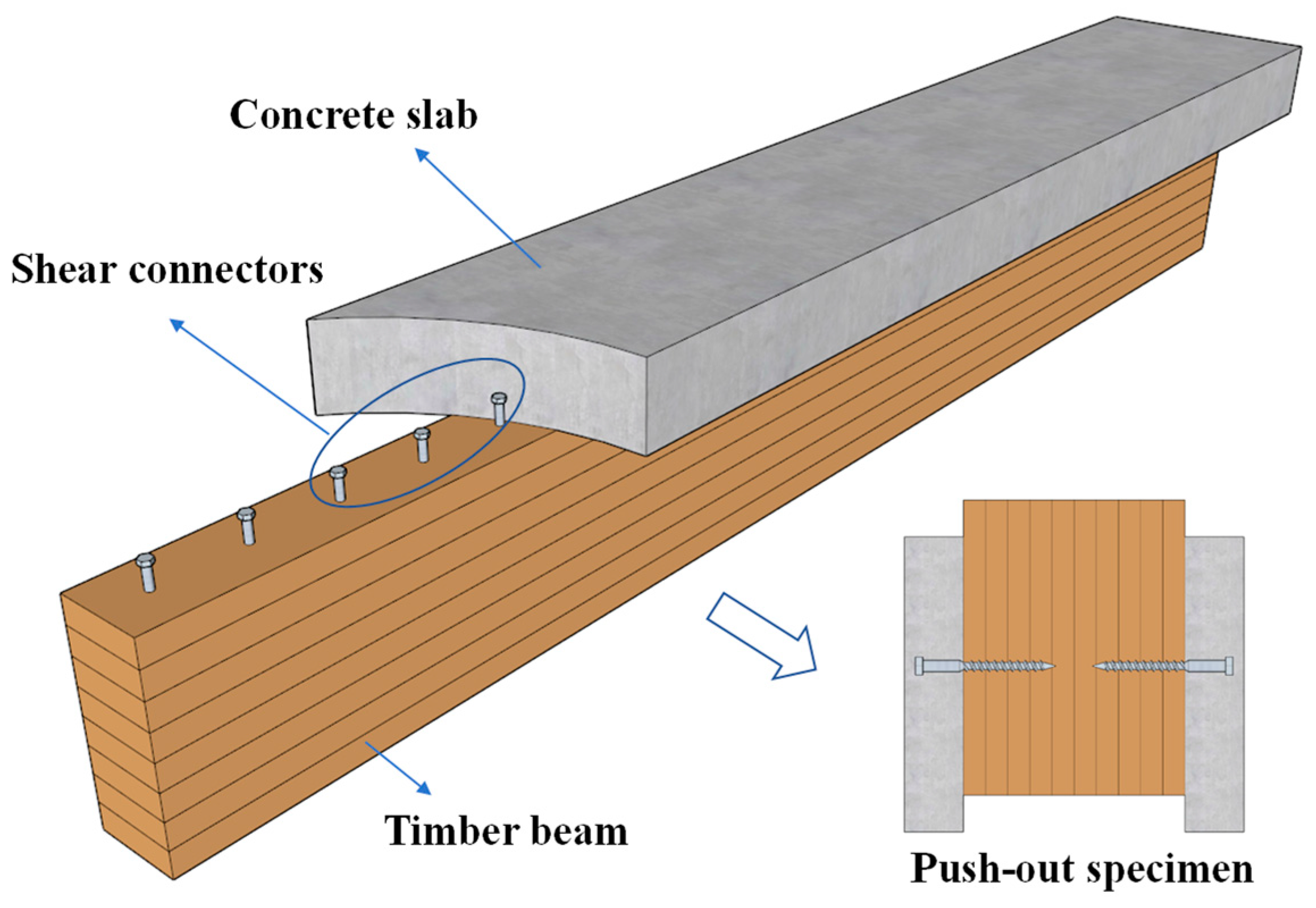
Figure 1. Diagram of TCC beam and its connection systems.
Buildings 15 02458 g001
Figure 2. Interface diagrams of four typical screw arrangements: (a) vertical screw; (b) shear–tension screw; (c) shear–compression screw; (d) bidirectional screws.
Buildings 15 02458 g002
Figure 3. Loading diagram and procedure: (a) diagram; (b) loading procedure in EN 26891 [42].
Buildings 15 02458 g003
Figure 4. Frequency of characteristic parameters.
Buildings 15 02458 g004
Figure 5. Correlation between each input feature.
Buildings 15 02458 g005
Figure 6. Diagram of ML modeling process.
Buildings 15 02458 g006
Figure 7. Influence of different hyperparameters on prediction accuracies: (a) DT; (b) RF; (c) AdaBoost; and (d) GBRT.
Buildings 15 02458 g007
Figure 8. Comparisons between prediction and experimental results (kN/mm): (a) DT model; (b) RF model; (c) AdaBoost model; (d) GBRT model.
Buildings 15 02458 g008
Figure 9. Influence of different input features.
Buildings 15 02458 g009
Figure 10. Features impact analysis: (a) screw diameter; (b) screw penetration depth; (c) screw arrangement methods; (d) screw inclination angle; (e) screw type; (f) timber density; (g) timber type; (h) interlayer thickness; (i) concrete compressive strength; (j) concrete type.
Buildings 15 02458 g010aBuildings 15 02458 g010b
Figure 11. Case studies of two typical experimental specimens: (a) specimen CBIS16-200-4; (b) specimen S-M8-200-45-B.
Buildings 15 02458 g011
Table 1. Hyperparameter space range.
MethodsHyper-Param1Hyper-Param2Hyper-Param3
DTmax_depth(1, 20)/13max_leaf_nodes(1, 100)/69min_samples_leaf(1, 10)/1
RFn_estimators(1, 500)/18max_depth(1, 20)/11min_samples_leaf(1, 10)/1
AdaBoostn_estimators(1, 500)/21Learning_rate(0, 1)/0.3230/
GBRTn_estimators(1, 500)/431max_depth(1, 10)/3learning_rate(0, 0.5)/0.3096
Table 2. Prediction accuracy of ML models adopted.
IndexesR2MAERMSEMAPE (%)
TrainingTestingTrainingTestingTrainingTestingTrainingTesting
DT0.98720.90761.51564.85742.60266.79427.3520.09
RF0.94210.88732.69025.17445.53267.503711.0223.48
AdaBoost0.87510.81766.18257.49098.12539.545441.1154.36
GBRT0.98790.91971.38704.22552.53386.30646.3818.71
Table 3. Examples of the influence of features on test results.
ReferencesFeaturePara. 1Pos. 1Result 1Para. 2Pos. 2Result 2
Tao et al. [26]fc40.8Lines 41–4542.9260.0Lines 26–3057.91
Jiang et al. [54]fc18.2Line 14516.1122.8Line 14624.87
Du et al. [50]α45Lines 5–614.3990 Lines 11–139.49
Derikvand [55]α30Line 20864.8060Line 21032.00
Appavuravther [22]ds8Lines 52–546.2510Lines 55–579.62
Marchi et al. [18]ds8Lines 122–1256.9112Lines 130–1338.20
Mirdad et al. [44]ρt0.574Line 17559.740.455Line 19053.69
Mirdad et al. [44]ti0Line 18727.885Line 18817.18
Jorge et al. [52]ti0Line 20110.125Line 20214.60
Table 4. Accuracy comparison between ML and design models.
MethodsData SetR2RMSEMAEMAPE (%)
GBRTTesting set0.91974.22556.306418.71
AdaBoostTesting set0.81767.49099.545454.36
Eurocode 5 [29]Vertical and shear–
compression screws
0.24902.86022.044018.04
Dias [79]Vertical screw0.15846.74536.253274.63
Wilkinson [81]Vertical screw−1.449211.509410.5199110.65
Du et al. [51]Vertical and shear–
tension screws
−0.386432.105418.961056.72
Tao et al. [26]Bidirectional screws0.102815.780111.252819.45
Disclaimer/Publisher’s Note: The statements, opinions and data contained in all publications are solely those of the individual author(s) and contributor(s) and not of MDPI and/or the editor(s). MDPI and/or the editor(s) disclaim responsibility for any injury to people or property resulting from any ideas, methods, instructions or products referred to in the content.