Experimental and Numerical Assessment of the Thermal Bridging Effect in a Reinforced Concrete Corner Pillar

Abstract

This paper discusses experimental and simulated data regarding the thermal bridging effect in a reinforced concrete corner pillar, which belongs to a building dating back to the 1980s and located in Southern Italy. The thermal field determined by the concrete pillar corner has been evaluated, introducing an experimental procedure based on both direct measurements and indirect observations of the inner superficial temperature by means of thermal imaging techniques and surface temperature probes. Moreover, indoor and outdoor air temperature and relative humidity were measured to provide suitable boundary conditions in the numerical simulations, performed with a commercial software tool widely used in Italy based on 2D finite element techniques. The experimental measurements show that, at more than 50 cm from the corner, the surface temperatures become almost constant, meaning that the thermal bridging effect becomes less evident. However, the surface temperature in the corner is around 1.5 °C lower than in the undisturbed flanking walls. In terms of local heat flux, the discrepancy between simulations and measurements is below 3%. Finally, this paper verifies the effectiveness of External Thermal Insulation Composite System (ETICS) renovation in reducing the thermal bridging effect of the corner pillar. The results also include the calculation of the linear thermal transmittance with a series of relations available in well-known atlases for thermal bridges and show that these relations are more reliable in the case of uninsulated pillar than for the insulated one.

1. Introduction

According to a recent estimation by the Odyssee-Mure project, buildings are responsible for about 39% of the final energy demand in the European Union [1], with 2/3 of this share coming from households. Such a significant energy consumption by the existing building stock can be mostly attributed to the poor thermal performance of their envelope, especially for those buildings built before 1990, when current EU regulations addressing energy efficiency in buildings were not in force. Thus, it is possible to estimate that around 75% of the current EU building stock is not energy efficient [2].

A non-negligible contribution to heat losses in buildings comes from thermal bridges. Thermal bridges are those parts of the building envelope where the otherwise uniform thermal resistance is modified either by a local change in the geometry or by penetration of the building envelope by materials with different thermal conductivity [3]. Common examples of thermal bridges are balconies, floor-to-wall connections, corners, and window sills/reveals. The impact of thermal bridges on the energy balance is particularly relevant in buildings with reinforced concrete (RC) structures. Indeed, the thermal conductivity of RC ranges from 2.0 to 2.5 W∙m⁻¹∙K⁻¹, depending on the quantity of reinforcing steel bars, while other common building materials (e.g., cement screed, mortar, bricks, non-reinforced concrete) have a much lower thermal conductivity (namely, between 0.4 and 1.0 W∙m⁻¹∙K⁻¹). Hence, RC beams, pillars, and balconies locally modify the temperature field, increase heat transfer, and determine “cold points” where mould growth can occur [4].

While the addition of thermal insulation to the building envelope is an effective way to drastically reduce the transmission heat losses through walls and slabs, only an accurate correction of the thermal bridging details may lead to a significant reduction in their impact [5]; thus, thermal bridges may become particularly important also in well-insulated buildings where the construction detailing has not been designed with good accuracy [6]. For instance, Ilomets et al. underlined that neglecting thermal bridges can lead to underestimating by 23% the transmission heat losses in an uninsulated building in Northern Europe, but ETICS renovation is likely to even increase this share up to 34% in case of “bad practice” correction, especially because of window lintels and balconies. Instead, “good practice” ETICS insulation reduces thermal bridges to around 10% of the transmission heat losses [7].

Some studies analysed thermal bridges in buildings with lightweight concrete or clay bricks and RC structures and demonstrated that in these buildings, the most important thermal bridges were due to balconies, pillars, and the contact between the wall and window [5,8,9]. Curto et al. provided a detailed analysis of thermal bridges in a building with tuff blocks and RC structures and drew up a list of “good practice” precautions to insulate the building and reduce the transmission heat losses in the thermal bridges to 9% of the total [10]. Thermal breakers emerge as an interesting, innovative solution to correct the thermal bridge between exterior walls and concrete slabs, both with and without a balcony, leading to a reduction in the space heating demand ranging from 5% to 25% according to the climate and the building geometry [8,11,12,13,14].

Moreover, it is interesting to underline that in Southern Europe, “good practice” insulation with corrected thermal bridges can reduce the space heating demand of a building by around 30% in the winter, but the effects of thermal bridge correction in the summer is practically negligible, because of the limited temperature gradient between indoors and outdoors [15,16,17]. However, in very hot climates such as in the Gulf area, the intense solar radiation hitting the structural elements, especially in the west façades, makes heat gains through thermal bridges not negligible in the summer; covering the exposed structural elements with a layer of insulation of no more than 100 mm can prevent such a negative effect [18]. Finally, the mitigation of thermal bridges is also of crucial importance in the refurbishment of traditional buildings, as pointed out by Cirami et al. [19].

Now, given the importance of thermal bridges and their non-negligible impact on the overall heat losses in buildings, their evaluation must be accurately carried out with reliable tools, such as via numerical finite element analysis or by means of thermal bridge atlases compliant with the recently updated Standard EN ISO 14683:2017 [20]. Previously adopted approximate methods, e.g., based either on a fixed percentage increase applied to the transmission heat losses or on a fixed surcharge to the U-value, regardless of the building’s features, are no longer admitted [21].

The current thermal bridge calculation tools aim at assessing the linear thermal transmittance (ψ): this parameter measures the increase in the transmission heat losses caused by a thermal bridge per unit length if compared to a thermally undisturbed envelope with parallel isothermal lines. Only a few years ago, commercial finite element numerical tools were not widespread; thus, the linear thermal transmittance of thermal bridges was mainly determined through atlases and abacuses, including a large variety of common cases.

For instance, the CENED abacus, published in 2011 under the initiative of the Lombardy Region and based on the research carried out by Politecnico of Milan [22], includes more than one hundred thermal bridges with equations to calculate their linear thermal transmittance (ψ) as a function of technical parameters like the wall thickness, the U-value, and the thermal conductivity of the insulating material (if any). One more atlas available in Italy is edited by Edilclima [23]; this includes a collection of common thermal bridges, and their linear thermal transmittance is reported in tabular form. However, no analytic relations are available. The Standard EN ISO 14683:2017 also includes default ψ-values for a limited range of commonly occurring types of two-dimensional thermal bridges, which can be used when there is no detailed information about the specific building node [20]; other available catalogues are the Swiss atlas distributed by the Office Federal de l’Energie OFEN [24] and the Passive House Institute atlas [25].

All these catalogues consider recurring construction techniques and are sufficiently reliable (accuracy ±20%) if the dimensions and the thermal properties of the included thermal bridges are similar—or less favourable—to those of the real detail; otherwise, catalogues may become very inaccurate and usually underestimate the heat losses through the thermal bridge [26,27].

On the contrary, the finite element analysis has the advantage of avoiding any geometric limitations and allows for an accurate calculation of the depicted construction detail according to the Standard EN ISO 10211:2017, with an error below ±5% [3]; furthermore, it provides both the heat flux and the temperature distribution in the building component, thus giving information on the possible occurrence of mould growth [10]. The use of 2D finite element numerical tools to determine the linear thermal transmittance has recently become very common, even in non-scientific applications such as for the release of Energy Performance Certificates. Indeed, many commercial software tools now include suitable plug-ins to support this.

The present paper shows experimental and simulated analyses regarding the thermal field in a reinforced concrete protruding corner pillar, which belongs to a building with uninsulated lightweight concrete walls. The building dates back to the 1980s; it is located in Southern Italy and displays a very common building solution in Italy, at least until the first comprehensive energy-saving regulation was issued in 1991. The proposed investigation aims to define an experimental procedure to evaluate the thermal bridging effect using both direct measurements and indirect observations of the inner surface temperature around the reinforced concrete protruding corner pillar. In particular, the internal surface temperatures of both the corner pillar and the adjacent building elements were measured by using several Pt 1000 probes and a thermal imaging camera. Indeed, infrared thermography has been recently recognized as a useful, non-invasive method to provide both qualitative and quantitative measures of the actual thermal bridging performance [28,29]. The infrared thermography allows for a precise visualization of the temperature field around the corner pillar, which is here enforced by the direct measurements of the surface temperatures in a grid of points within the investigated area. The thermal bridge was also studied numerically through a commercial software tool widely used in Italy, based on 2D finite element techniques. Moreover, the effectiveness of ETICS renovation in reducing the thermal bridging effect of the corner pillar has been verified.

The findings of this paper demonstrate that the proposed experimental practice can provide a reliable assessment of the thermal field around corner pillars, highlighting the extension of the coldest area, as well as the increased heat flux transmitted through the thermal bridge. One of the strengths of the proposed procedure is its simplicity, both in terms of timing and equipment. Thus, the proposed approach could be followed by technicians to quantify the thermal bridging effect in existing buildings with reinforced concrete structures as well as to verify the efficacy of the retrofit interventions for the mitigation of this kind of thermal bridge. Moreover, this paper casts light on the ability of catalogues and atlases to reliably calculate the so-called “linear thermal transmittance” for this type of thermal bridge, both in the case of insulated and uninsulated walls, thus providing useful methodological information for a reliable assessment of corner pillars in a very high number of buildings.

2. Materials and Methods

The case study here addressed a corner pillar made with reinforced concrete that belonged to a detached house with uninsulated hollow concrete blocks built in the 1980s. The building is in Ragalna (province of Catania), a municipality located on the Southern slope of Mount Etna, at 830 m above sea level (Lat: 37°38′; Long: 14°56′). According to the Italian Presidential Decree DPR 412/93 [30], the Heating Degree Days attributed to this municipality are HDD = 1879 °C∙day (climate zone D). The observed mean minimum daily air temperature in the winter is 3 °C, whereas the mean maximum daily temperature in the summer is 28 °C.

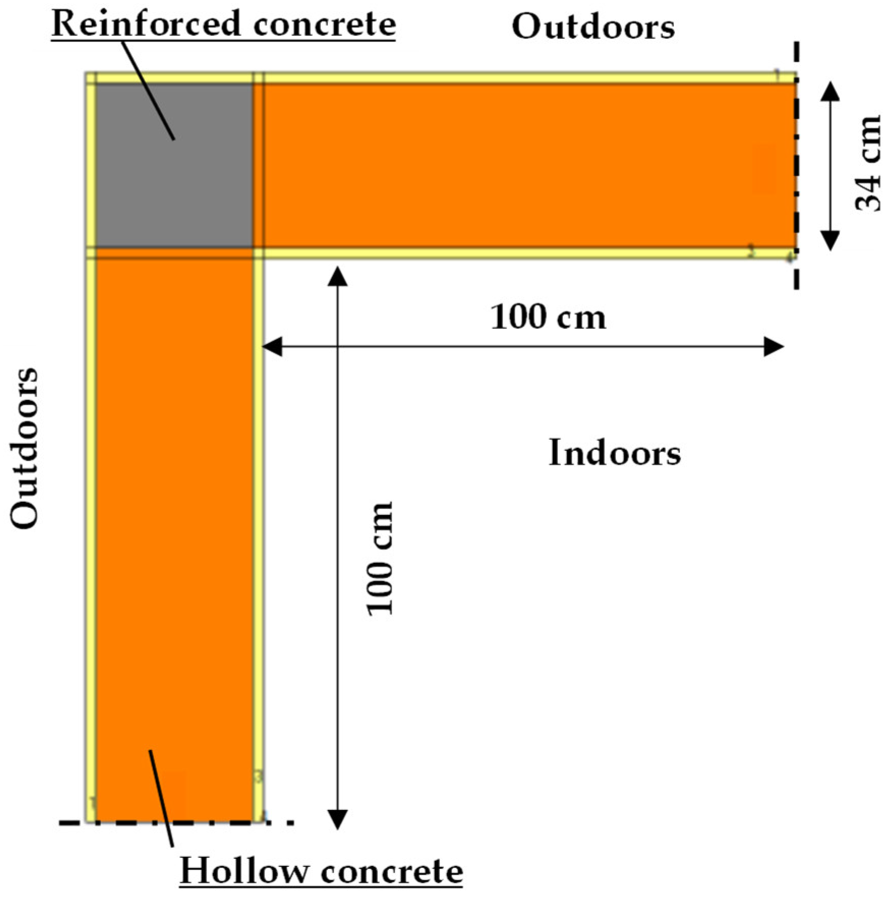
2.1. A 2D Numerical Modelling

The selected thermal bridge has been numerically simulated with the software tool “IRIS”, provided by ANIT (National Association for Thermal and Acoustic Insulation) [31]. The two-dimensional model built in IRIS is shown in Figure 1; as suggested by the Standard EN ISO 10211:2017 [3], the length of the two walls that constitute the thermal bridge (flanking elements) is at least equal to the greater number between 100 cm and is three times the thickness of the flanking elements (here, 34 cm). The thermal field in the modelled detail is supposed not to vary along the third dimension and is determined in steady-state conditions.

The thermal properties of the materials set in the simulations are reported in Table 1. The hollow concrete blocks are described as a “full” layer with equivalent thermal conductivity and density; this means that the equivalent layer has, for the same given thickness (30 cm), the same thermal resistance and surface mass as the real hollow blocks, including 12-mm mortar joints between the blocks. The reported values are taken from an Italian Standard [32] and refer to hollow blocks with 50% void area, typically used in the 1980s in Southern Italy. The internal and external overall surface thermal resistance values have been set to R_si = 0.13 m²∙K∙W⁻¹ and R_se = 0.04 m²∙K∙W⁻¹, respectively [33]. The resulting wall thermal transmittance is U_WALL = 1.26 W∙m⁻²∙K⁻¹.

Regarding the boundary conditions used in the simulations, indoor and outdoor temperatures are given the same values observed during the measurement campaign, as explained in Section 2.2. As a result, the numerical simulation provides the temperature values in all points of the building detail and the transmitted heat flux (q) per unit length. The tool is validated against the cases provided in Appendix C of the Standard EN ISO 10211:2017, showing an error below 0.1 °C on the minimum temperature.

Figure 1. Cross section of the simulated 2D building detail.

Figure 1. Cross section of the simulated 2D building detail.

Table 1. Thermal properties of the selected building materials.

Material	Thickness	Conductivity	Density
	[cm]	[W∙m−1∙K−1]	[kg∙m−3]
Inner cement plaster	2	0.70	1300
Hollow concrete blocks [32]	30	0.55	770
Reinforced concrete	30	2.50	2300
Outer gypsum plaster	2	0.40	1800

Table 1. Thermal properties of the selected building materials.

Material	Thickness	Conductivity	Density
	[cm]	[W∙m−1∙K−1]	[kg∙m−3]
Inner cement plaster	2	0.70	1300
Hollow concrete blocks [32]	30	0.55	770
Reinforced concrete	30	2.50	2300
Outer gypsum plaster	2	0.40	1800

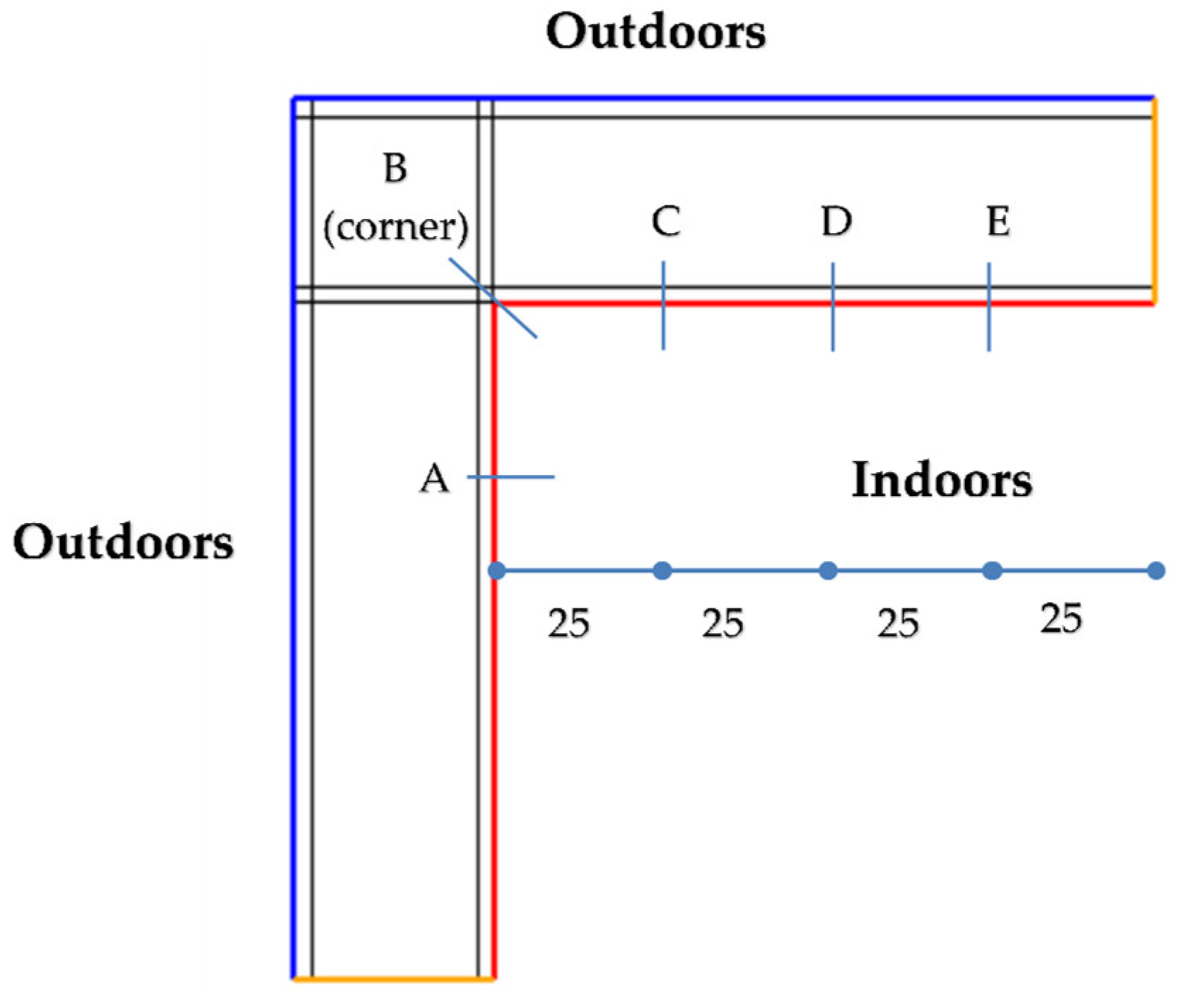
2.2. Experimental Measurements

Several devices were used in this study to measure the internal surface temperatures, as well as the indoor and outdoor conditions. The measurement campaign was carried out on the 22nd of February 2022, in the morning; the two walls are oriented north and west, but they are constantly shaded by a porch and are not hit by direct solar radiation. The room was preliminarily warmed for around two hours with a fan heater until a sufficient temperature difference was observed between the indoor and outdoor environment, and the walls could show a reasonably fully developed and steady thermal field. Once these conditions were achieved, all measured parameters were collected for ten minutes with an acquisition step of one minute, which was deemed sufficient to identify and describe an almost steady behaviour. More in detail, indoor and outdoor conditions were acquired using a Testo 645 high-precision humidity/temperature measuring instrument equipped with a Pt100 probe (Figure 2), with the following features:

• Temperature range: from −200 °C to +200 °C;
• Temperature resolution: ±0.1 °C;
• Temperature accuracy: ±0.2 °C;
• Relative Humidity range: from 0% to +100%;
• Relative Humidity resolution: ±0.1%.

The mean air temperature and relative humidity over the acquisition period are as follows:

• Indoors: T_I = 17.0 °C and RH_I = 52.1%;
• Outdoors: T_E = 10.7 °C and RH_E = 58.4%.

Instead, two ThermoZig dataloggers, manufactured by Carlesi Strumenti (Bologna, Italy), were used to measure the internal wall surface temperature at several different points: while one datalogger was equipped with two Pt1000 (Class A) temperature probes, the second one had a Pt1000 temperature probe plus a heat flux sensor (Figure 2), which was, however, only used to collect a surface temperature value. The features of the probes are as follows:

• Temperature range: from −50 °C to +150 °C;
• Temperature resolution: ±0.01 °C;
• Temperature accuracy: ±0.15 °C.

Figure 2. ThermoZig datalogger (left) and Testo 645 digital humidity/temperature measurement device (right).

Figure 2. ThermoZig datalogger (left) and Testo 645 digital humidity/temperature measurement device (right).

Figure 3 and Figure 4 show the position of the probes: two of them were placed at 25 cm from the corner on both sides in order to verify possible asymmetries; two more probes were placed at 50 cm and 75 cm from the corner, on the same side. All probes were positioned at the height of 1.5 m, that is to say, half the room height; no probe was placed in the corner.

Moreover, when dealing with thermal bridges, using a thermal imaging camera allows for a more comprehensive view of the thermal bridging effect and provides a further reference for the assessment of the local heat transfer. Thus, the thermal field on the internal wall surface was investigated through a thermal imaging camera (Thermacam B4) manufactured by Teledyne Flir LCC (Wilsonville, OR, USA) with the following performance parameters:

• Resolution: 320 × 240 pixels;
• Thermal sensitivity: 0.08 °C at 30 °C;
• Spectral range: 7.5 to 13 μm;
• Temperature range: from −20 °C to +55 °C;
• Temperature accuracy: ±2 °C.

The thermal emissivity was set at ε = 0.93. Using a thermal imaging camera is appropriate when the structures are preliminarily warmed up and when no solar radiation influences the thermal field observed with the camera. This justifies the choice of both the measurement time (early morning) and the position of the investigated walls (north and west fronts).

In this paper, the measured surface temperature values coming from the two different instruments will be compared to the simulated values, and the consequences of the possible differences in the assessment of the heat losses will be discussed.

Figure 3. Position and labelling of the points where the inner surface temperatures are measured (dimensions in cm).

Figure 3. Position and labelling of the points where the inner surface temperatures are measured (dimensions in cm).

Figure 4. Picture of the probes installed on the wall surface.

Figure 4. Picture of the probes installed on the wall surface.

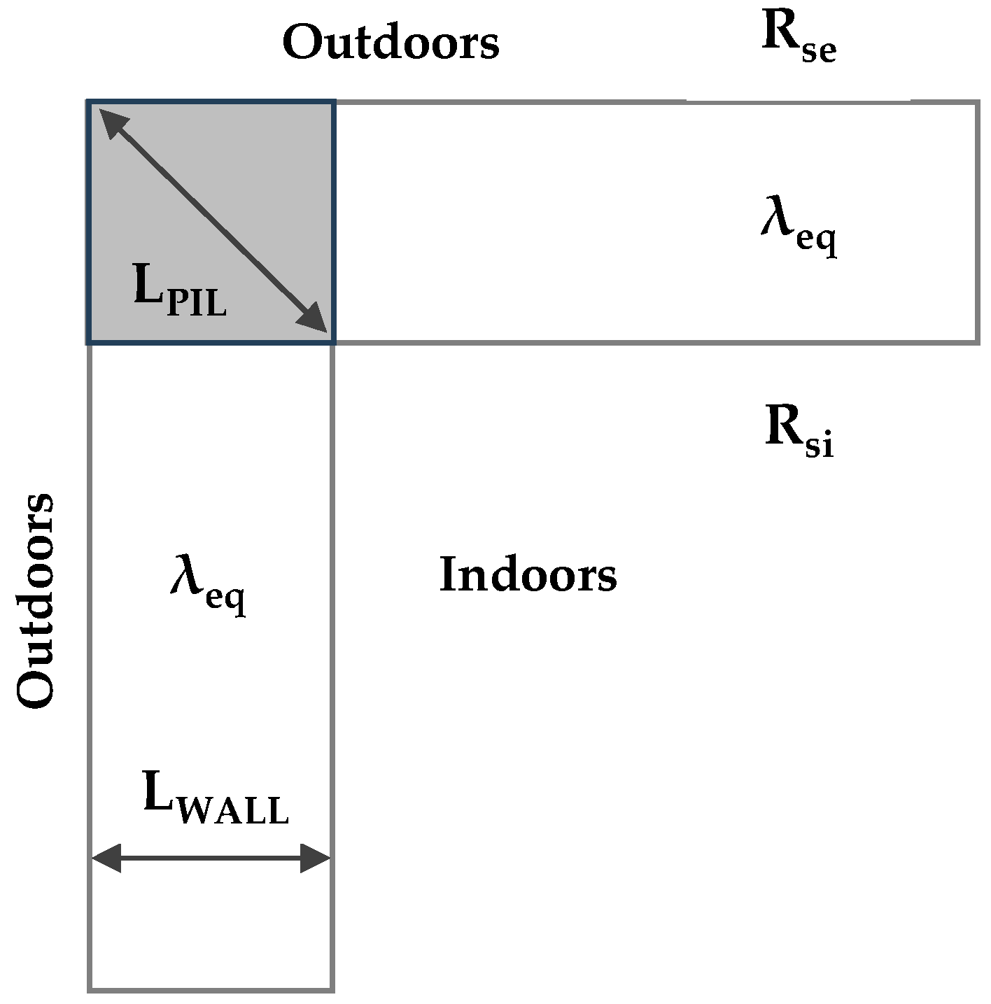
2.3. Determination of the Linear Thermal Transmittance

The first way to determine the linear thermal transmittance consists of elaborating on the results of the numerical simulations described in Section 2.1. Indeed, once the transmitted heat flux per unit length (q) is calculated, the linear thermal transmittance can be determined as follows [3]:

$$\psi =\frac{q}{\left(T_I-T_E\right)}-U·A$$

(1)

In Equation (1), (A) is the area of the flanking elements per unit length that can be measured between the finished external or internal faces, giving rise to two different values of the linear thermal transmittance, respectively identified as ψ_E and ψ_I.

Moreover, the CENED abacus [22] proposes the relations reported in Equations (2) and (3). The thermal bridge is identified via the code ASP.004 and is described by the parameters shown in Figure 5. The “non-dimensional” thermal transmittance U* is the ratio of two U-values, respectively referred to as the diagonal of the pillar (U_PIL) and to the wall (U_WALL), whereas the “equivalent thermal conductivity” (λ_eq) refers to the wall, but it does not include any insulation layers, if available.

$${\psi }_E=0.075+0.025\cdot U^{*}-1.056\cdot {\lambda }_{eq}$$

(2)

$${\psi }_I=0.350-0.003\cdot U^{*}+0.103\cdot {\lambda }_{eq}$$

(3)

On the other hand, in the Edilclima atlas [23], the case which is closest to the investigated thermal bridge is C15 (“Joint between two walls with distributed thermal insulation and uninsulated protruding pillar”); the linear thermal transmittance is assigned for nine different combinations of wall thickness (25 cm, 30 cm and 40 cm) and U-value (0.32, 0.73 and 1.3 W∙m⁻²∙K⁻¹). It is worth highlighting that this atlas only provides the “outer” linear thermal transmittance ψ_E; furthermore, the thermal conductivity of reinforced concrete elements is set by default to λ_RC = 2.0 W∙m⁻¹∙K⁻¹ and cannot be modified.

A further possible reference to calculate the linear thermal transmittance of a corner pillar comes from an outdated French regulation [34]. Here, the linear thermal transmittance of the investigated thermal bridge—actually, with hollow bricks in place of the lightweight concrete blocks—is provided as a function of the wall thickness. Other atlases available in the literature—including the Standard EN ISO 14683:2017—as well as the more recent versions of the French regulations, do not consider the case of a reinforced concrete corner pillar.

3. Results and Discussion

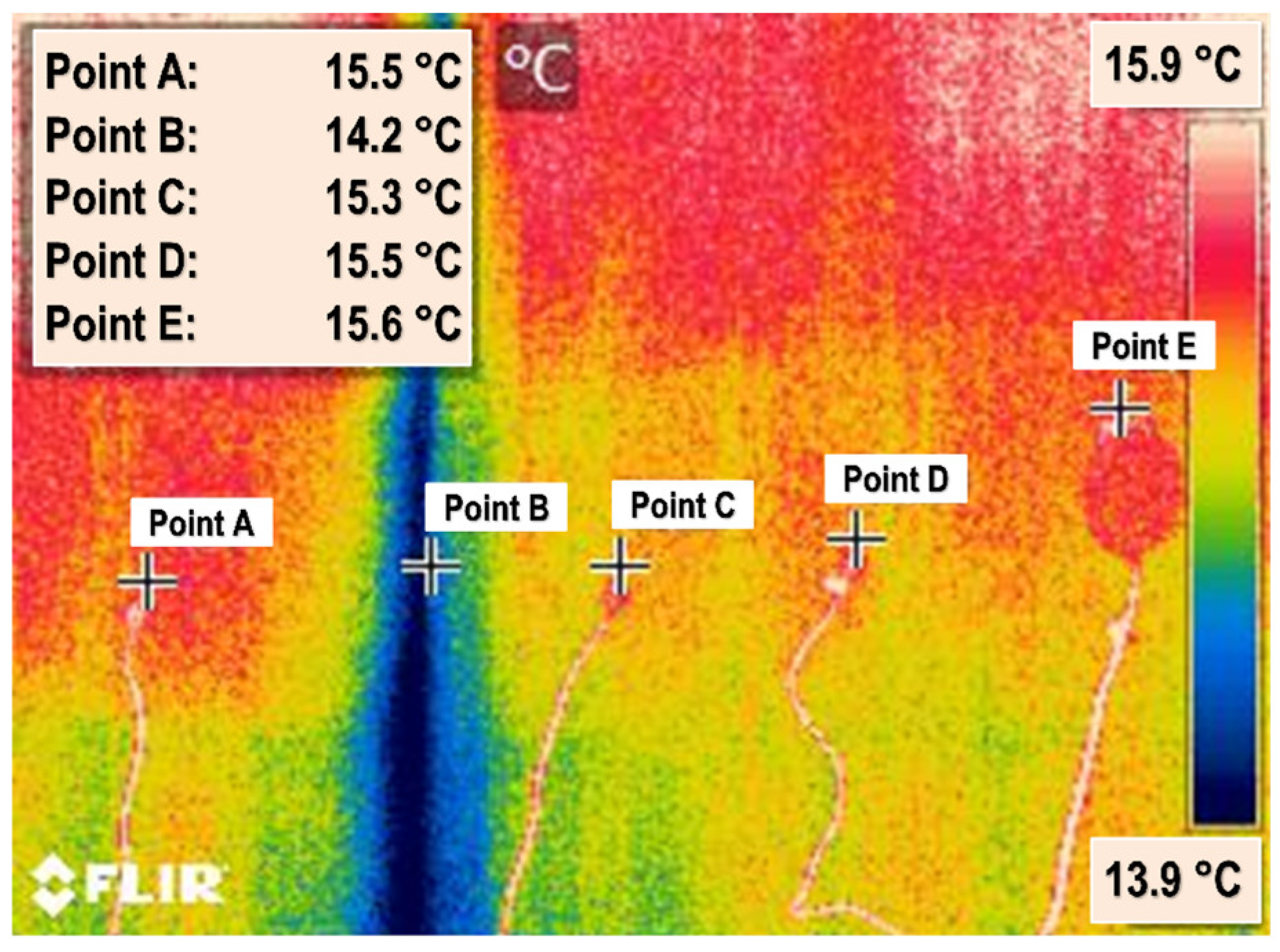
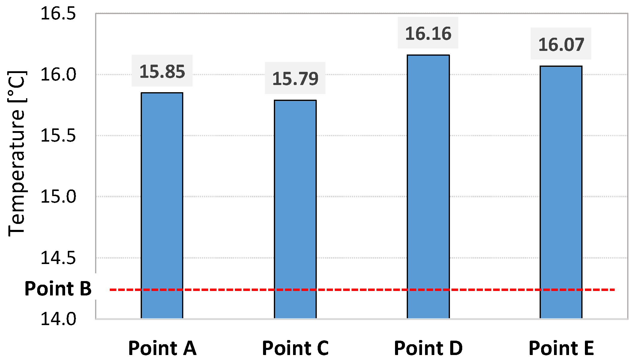
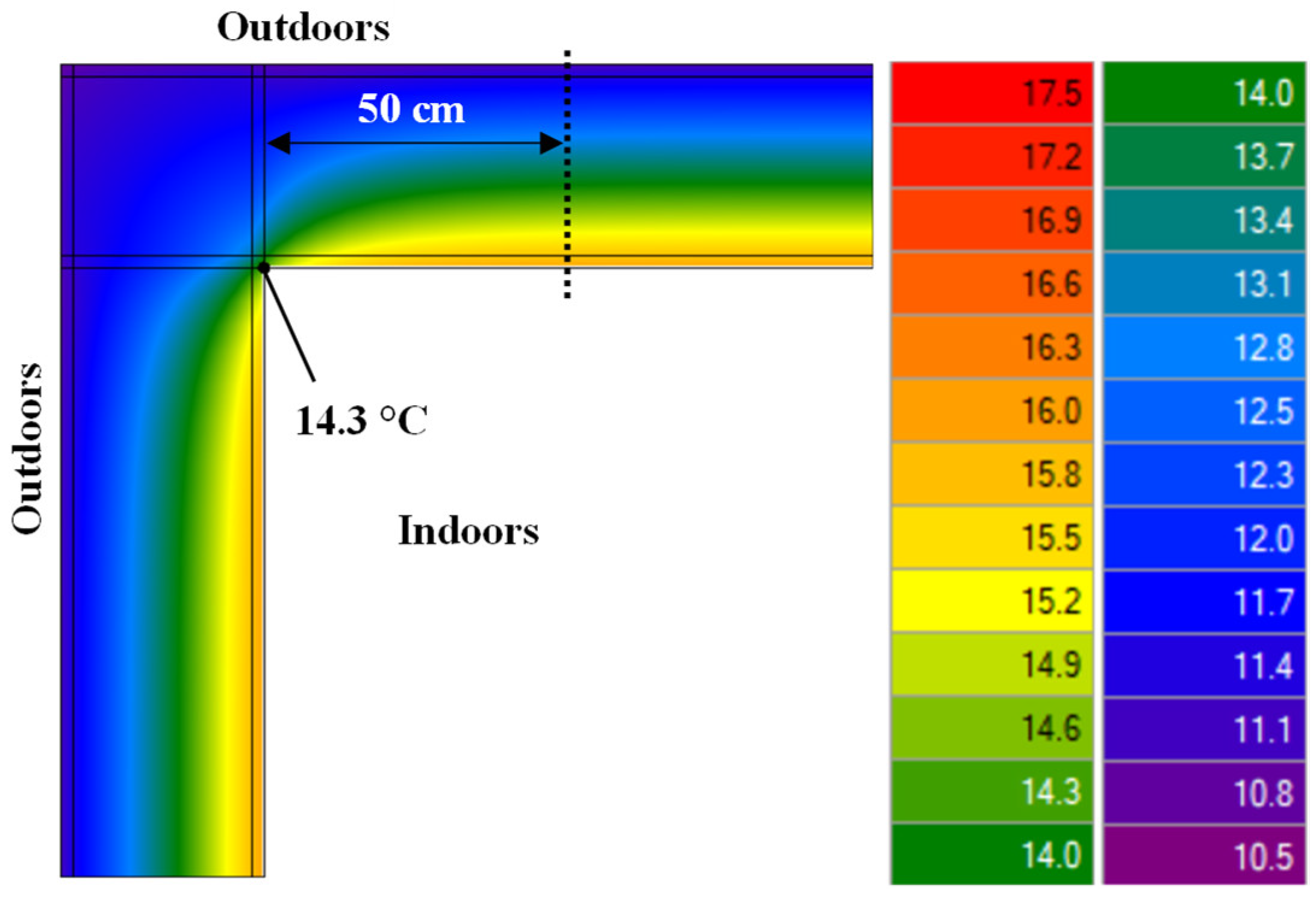
3.1. Surface Temperature

This section discusses the comparison among the surface temperature values determined through the various techniques described in Section 2, both experimentally and numerically. Starting from the thermal imaging survey, Figure 6 shows the thermal image taken in the middle of the measuring campaign five minutes after the first data acquisition. The thermal image allows for visualizing the thermal bridging effect, with the coldest point in the corner (Point B) reaching 14.2 °C along the horizontal plane where the ThermoZig probes belong. The thermal image also shows a slight asymmetry, with the left-hand side (Point A) being only 0.2 °C warmer than the corresponding point on the right-hand side (Point C). The surface temperature tends to become stable after point D, farther than 50 cm from the corner: the maximum observed difference in terms of surface temperature (from Point E to Point B, in the corner) amounts to 1.4 °C. Finally, a slight gradient in the surface temperature can be observed along the vertical direction, possibly due to buoyancy effects.

On the other hand, Figure 7 shows the mean values of the surface temperatures measured by the four ThermoZig probes during the ten-minute experiment (no probe has been installed in Point B in the corner). Figure 7 confirms that Point A and Point C, both at 25 cm from the corner, show almost the same temperature: indeed, Point A on the left-hand side keeps at slightly higher values (+0.06 °C on average). These two points are 0.3 °C colder than Point D, placed 25 cm farther. Then, Point D and Point E have practically the same temperature, thus suggesting that the thermal bridging effect becomes negligible beyond 50 cm from the corner.

Figure 6. Thermal image and corresponding surface temperatures in the five selected points.

Figure 6. Thermal image and corresponding surface temperatures in the five selected points.

Figure 7. Mean surface temperatures measured by the ThermoZig probes.

Figure 7. Mean surface temperatures measured by the ThermoZig probes.

Furthermore, Figure 8 shows the temperature distribution inside the corner pillar and the flanking elements resulting from the 2D numerical simulation. The simulation relies on a subdivision in 645 elements, which provided a variation of less than 0.05% on the total heat flux compared with a simulation based on 384 elements. Here, it is evident that not only does the surface temperature become stable farther than 50 cm from the corner, but that this is the distance after which the thermal bridging effect vanishes, and all isothermal lines become parallel. The RC pillar is signify/cantly colder than the adjacent walls; indeed, almost the entire pillar keeps below 12 °C, while a local temperature increase is observed close to the corner, with a minimum surface temperature corresponding to 14.3 °C. Finally, Figure 9 proposes a comparison between measured and simulated results. There is a very good agreement between numerical simulations and ThermoZig measurements, with a discrepancy in the order of 0.1 °C, while the thermal imaging tends to underestimate the surface temperatures, with a difference of around 0.5 °C from the simulations emerging in Point D and Point E. These results must be interpreted considering the temperature probes’ accuracy: on the one hand, this is 0.15 °C for the Pt1000 ThermoZig probes (Carlesi Strumenti, Bologna, Italy), which is the same order of magnitude as the discrepancy between measurements and numerical simulations. On the other hand, the accuracy of the thermal imaging camera is 2 °C, which may explain the higher discrepancy obtained using this kind of instrument.

3.2. Transmitted Heat Flux

Based on the internal surface temperature values collected by the ThermoZig dataloggers, one can also estimate the heat flux (q) locally exchanged by the surface of the investigated wall per unit length in steady-state conditions and compare it to the corresponding result of the numerical simulation. Indeed, given the symmetry of the component, which is confirmed by the very close temperature values in Point A and Point C, the following set of equations holds. The ratio behind these equations is that the two symmetrical adjacent walls are divided into four equal elements (25 cm each); the surface temperature attributed to each element is the average of the values measured at its extreme points.

$$q=2\cdot \left(q_1+q_2+q_3+q_4\right)$$

(4)

$$q_1=\frac{0.25}{R_{si}}\cdot \left[T_I-\frac{\left(T_{sB}+T_{sC}\right)}{2}\right]=3.8\frac{ W}{m}$$

(5)

$$q_2=\frac{0.25}{R_{si}}\cdot \left[T_I-\frac{\left(T_{sC}+T_{sD}\right)}{2}\right]=2.2 \frac{W}{m}$$

(6)

$$q_3=\frac{0.25}{R_{si}}\cdot \left[T_I-\frac{\left(T_{sD}+T_{sE}\right)}{2}\right]=1.8 \frac{W}{m}$$

(7)

$$q_4=\frac{0.25}{R_{si}}\cdot \left[T_I-T_{sE}\right]=1.8 \frac{W}{m}$$

(8)

Since the temperature in Point B was not measured by the ThermoZig device, in Equation (5), the thermal imaging value is used as T_B. Moreover, Equation (8) implies that the temperature in Point E holds until the far end of the flanking element, which is reasonable due to the stabilization of the temperature values beyond 50 cm from the corner. According to this approach, which relies on experimentally measured temperatures, the estimated heat flux transferred by the thermal bridge with its flanking walls amounts to 19.2 W∙m⁻¹. Considering the accuracy in the measurement of the indoor air temperature T_I (0.2 °C) and the surface temperatures in the various points (0.15 °C), the uncertainty in the estimated heat flux according to Equations (4)–(8) is 1.4 W∙m⁻¹. On the other hand, the value provided by the numerical simulation in IRIS is 18.6 W∙m⁻¹, with a discrepancy of only 2.7% from the estimated central value.

3.3. Linear Thermal Transmittance

This section compares the linear thermal transmittance of the uninsulated corner pillar, determined through the various methods discussed in Section 2.3, including the numerical simulations in IRIS based on the approach reported in the Standard EN ISO 10211:2017.

Table 2. Linear thermal transmittance of the investigated thermal bridge, according to different sources.

Source	ψI (W∙m−1∙K−1)	ψE (W∙m−1∙K−1)
Numerical simulation (IRIS)	0.385	−0.471
CENED abacus	0.401	−0.456
Edilclima atlas	-	−0.380
French regulation (Th-K 77)	0.15	-

compares the various values.

On the one hand, the CENED abacus implies the calculation of the “equivalent thermal conductivity” (λ_eq) and the “non-dimensional thermal transmittance” (U*). Here, the above-mentioned parameters assume the values calculated using Equations (9)–(11), where the wall thickness is L_WALL = 0.34 m:

$${\lambda }_{eq}=\frac{L_{WALL}}{\left(\frac{1}{U_{WALL} }-R_{si}-R_{se}\right)}=0.545 \frac{W}{m\cdot K}$$

(9)

$$\begin{gathered} U_{PIL}={\left(R_{si}+\sum _{j=1}^3\frac{L_j}{{\lambda }_j}+R_{se}\right)}^{-1}={\left(0.13+\frac{0.028}{0.7}+\frac{0.424}{2.5}+\frac{0.028}{0.4}+0.04\right)}^{-1} \\ =2.22 \frac{W}{m^2\cdot K} \end{gathered}$$

(10)

$$U^{*}=\frac{U_{PIL}}{U_{WALL}}=1.76$$

(11)

Under these circumstances, Equations (2) and (3) can be used since they hold if 0.23 ≤ λ_eq ≤ 0.81 and 1.5 ≤ U* ≤ 4.5. On the other hand, the ψ-value derived from the Edilclima atlas refers to 30 cm thick walls with U = 1.3 W∙m⁻²∙K⁻¹, i.e., very close to the investigated configuration. Finally, in the French regulation, a thickness between 30 and 34 cm provides ψ_I = 0.15 W∙m⁻¹∙K⁻¹, but no data about ψ_E are available.

Table 2 comparison proves that the formulation available in the CENED abacus is reliable as it deviates from the detailed 2D numerical simulations by only 3%. On the other hand, the Edilclima atlas overestimates the heat losses in the corner pillar by around 20%. Finally, the outdated French standard cannot be considered reliable since it underestimates the linear thermal transmittance by more than 60%. The main reason is that these sources have some underlying hypotheses that do not always correspond to the current case study (for instance, the Edilclima atlas considers λ_RC = 2.0 W∙m⁻¹∙K⁻¹ for reinforced concrete, and this value cannot be modified). In all cases, the linear thermal transmittance is lower when using the external building dimensions (ψ_E); indeed, the heat loss surface is already overestimated, and a minor additional heat loss must be accounted for.

One further interesting result consists of defining the increase in the heat flux caused by the corner pillar if compared to a couple of real undisturbed uninsulated walls. Indeed, if one considers two real walls with an internal size A_I = 10.8 m² each (height H = 2.7 m, width W = 4 m), the heat losses in the absence of the thermal bridging effect (Q_noTB) would be determined as in Equation (12). Instead, taking the thermal bridge into account, one should adopt Equation (13):

$$Q_{n{o}_{TB}}=U_{WALL}\cdot \left(T_I-T_E\right)\cdot 2\cdot A_I=171.5 W$$

(12)

$$Q_{TB}=q_{n{o}_{TB}}+{\psi }_I\cdot \left(T_I-T_E\right)\cdot H=178.0 W$$

(13)

This result suggests that the RC corner pillar causes an increase of 3.8% in the local heat losses, thus confirming that thermal bridges associated with RC corner pillars in uninsulated walls have a relatively low impact on the heat losses while determining possible mould growth due to the low internal surface temperatures.

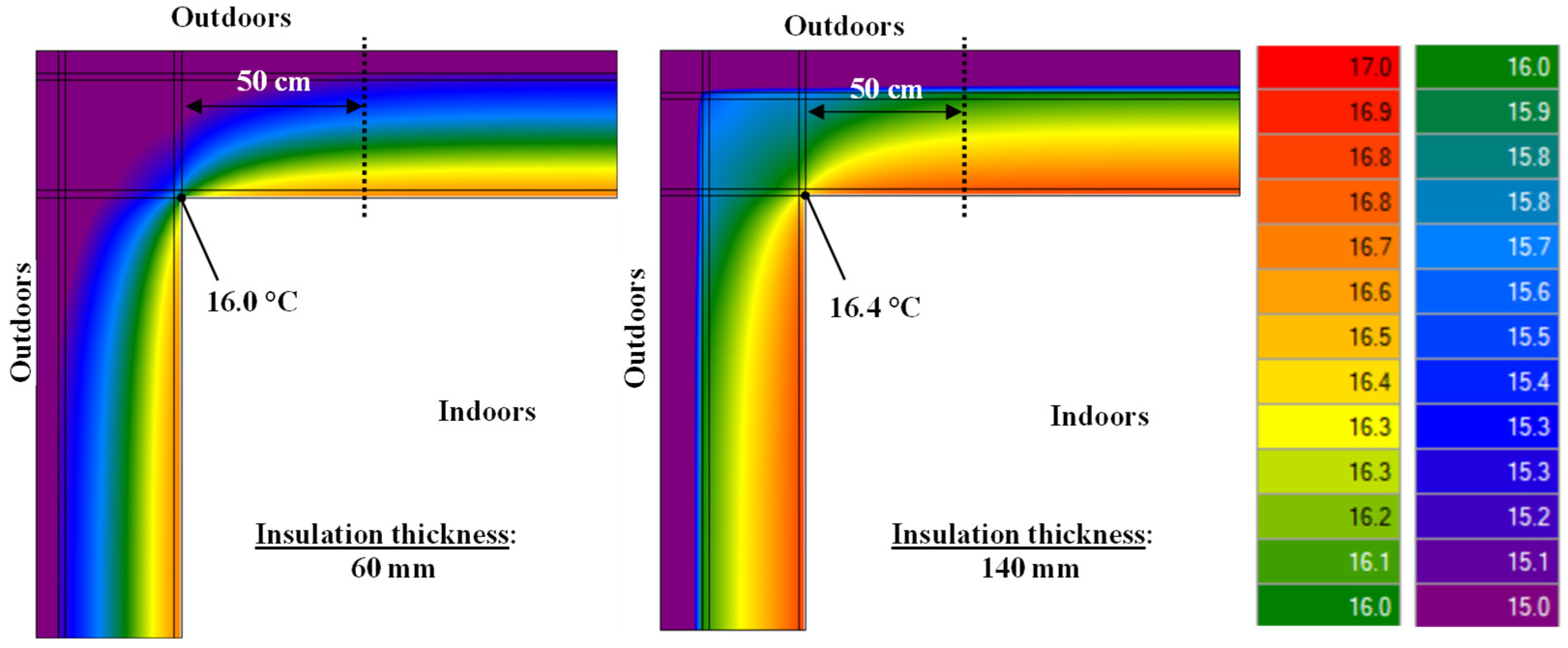
4. Effect of ETICS Renovation on Thermal Bridges

This section explores the effectiveness of ETICS insulation in reducing the thermal bridging effect in the RC corner pillar. To this aim, a layer of extruded polystyrene (XPS) with ρ = 40 kg∙m³ and λ = 0.035 W∙m⁻¹∙K⁻¹ is added on the external side of the wall; several different thickness values are tested, from 6 cm to 14 cm. The thermal performance of the insulated building detail is evaluated numerically by means of IRI, in terms of minimum internal surface temperature and linear thermal transmittance; for the sake of comparison, the latter is also assessed using the CENED abacus and the Edilclima atlas.

In particular, the CENED abacus considers the following set of equations to calculate the linear thermal transmittance of a protruding corner pillar with externally insulated walls, identified by the code ASP.005:

$${\psi }_E=-0.281+0.147\cdot U^{*}+0.143\cdot L_{WALL}$$

(14)

$${\psi }_I=0.385-0.116\cdot U^{*}-0.198\cdot L_{WALL}$$

(15)

Here, the wall thickness L_WALL and the “non-dimensional” thermal transmittance U*, calculated as in Equation (11), take the insulating layer into account. Equations (14) and (15) hold if 0.30 m ≤ L_WALL ≤ 0.65 m and 0.76 ≤ U* ≤ 1.18, which is the case of the investigated thermal bridge (U* = 0.78 to 0.87, L_WALL = 0.40 m to 0.48 m).

Coming to the Edilclima atlas, the relevant case is C14 (“Joint between two walls with continuous external insulation and insulated protruding pillar”).

Table 3. Linear thermal transmittance values (ψ_E) according to Edilclima atlas [23]—thermal bridge C14 (“Joint between two walls with continuous external insulation and insulated protruding pillar”).

	Linear Thermal Transmittance ψE
U-Value	Thickness = 30 cm	Thickness = 40 cm
0.70 W∙m−2∙K−1	−0.16 W∙m−1∙K−1	−0.21 W∙m−1∙K−1
0.60 W∙m−2∙K−1	−0.13 W∙m−1∙K−1	−0.17 W∙m−1∙K−1
0.50 W∙m−2∙K−1	−0.11 W∙m−1∙K−1	−0.14 W∙m−1∙K−1
0.40 W∙m−2∙K−1	−0.09 W∙m−1∙K−1	−0.11 W∙m−1∙K−1
0.30 W∙m−2∙K−1	−0.07 W∙m−1∙K−1	−0.09 W∙m−1∙K−1
0.20 W∙m−2∙K−1	−0.06 W∙m−1∙K−1	−0.07 W∙m−1∙K−1
0.10 W∙m−2∙K−1	−0.06 W∙m−1∙K−1	−0.06 W∙m−1∙K−1

The thickness refers to the wall without insulation, with λ_eq = 0.5 W∙m⁻¹∙K⁻¹.

reports the suggested values for the “outer” linear thermal transmittance ψ_E holding if the uninsulated portion of the wall has an equivalent thermal conductivity λ_eq = 0.5 W∙m⁻¹∙K⁻¹, i.e., only 10% lower than the investigated wall.

Table 4. Main parameters describing the thermal performance of the insulated corner pillar (the acronym NA indicates non-available data).

Insulation Thickness	6 cm	8 cm	10 cm	12 cm	14 cm
UWALL [W∙m−2∙K−1]	0.399	0.325	0.274	0.237	0.209
Minimum TSI (°C)	16.0	16.1	16.2	16.3	16.4
Linear thermal transmittance—external ψE (W∙m−1∙K−1)
Numerical simulation (IRIS)	−0.099	−0.083	−0.073	−0.067	−0.063
CENED abacus (case ASP.005)	−0.096	−0.098	−0.099	−0.098	−0.097
EDILCLIMA atlas (case C14)	−0.100	−0.085	−0.075	−0.070	−0.065
Linear thermal transmittance—internal ψI (W∙m−1∙K−1)
Numerical simulation (IRIS)	0.220	0.190	0.168	0.151	0.137
CENED abacus (case ASP.005)	0.205	0.205	0.204	0.201	0.199
EDILCLIMA atlas (case C14)	NA	NA	NA	NA	NA

resumes the various results; those pertaining to the Edilclima atlas were interpolated from Table 3 by considering a thickness of 34 cm and the U-values reported in the second row of Table 4 itself.

The results suggest that increasing the insulation thickness from 6 cm to 14 cm has a minor effect on the internal surface temperature, which changes from 16.0 °C to 16.4 °C; in any case, the ETICS allows for increasing this temperature by around 2.0 °C compared to the uninsulated corner pillar (point B in Figure 9), and this avoids the risk of mould growth on the internal surface. Moreover, higher insulation thickness means lower internal linear thermal transmittance (ψ_I): this effect is particularly evident in the numerical simulations (IRIS), while the results of the CENED abacus are not sensitive to the insulation thickness and show a non-negligible discrepancy from the detiled IRIS simulations, ranging from 7% underestimation (6 cm of insulation) to 50% overestimation (14 cm of insulation). On the contrary, the Edilclima atlas reflects very well the numerical predictions in this case. Previous studies highlighted that thermal bridge catalogues are not always very reliable: in some cases, their use allows for calculating the overall heat losses through thermal bridges with an error below 10%, while in other cases, very high discrepancies were observed [35].

Further interesting information comes from Figure 10, which shows the temperature distribution inside the insulated walls, resulting from IRIS simulations. Here, please consider that the size of the flanking elements is not the same as in the uninsulated thermal bridge (Figure 8): indeed, the flanking element must be at least three times as long as the wall thickness [3], leading to a length of 1.2 m and 1.44 m, respectively, with 6 cm and 14 cm of thermal insulation. The two diagrams show that in both cases, the isothermal lines become parallel at more than 50 cm, precisely at around 60 cm in the case of medium-thermal insulation (6 cm) and 70 cm in the case of high-thermal insulation (14 cm). Interestingly, Hallik et al. demonstrated that, in the case of a well-insulated building envelope with RC structures, the sufficient length of the flanking element to adequately calculate the linear thermal transmittance is equal to approximately the wall’s thickness [36]. In our study, this minimum distance approximates 1.5 times the wall thickness; by the way, it is confirmed that the minimum distance imposed by the Standard EN ISO 10211:2017 is, in many cases, excessive and that it could be reduced by around 50% to minimize computational time.

Finally, it is interesting to repeat the same exercise discussed at the end of Section 3.3, aimed at quantifying the local increase in the heat losses due to the thermal bridge between two real walls with an internal size A_I = 10.8 m² each. In the case of the ETICS application, the heat flux transferred with no thermal bridging—see Equation (12)—would range from 28.4 W (insulation: 14 cm) to 54.3 W (insulation: 6 cm). Instead, taking the thermal bridge into account, Equation (13) would provide heat losses ranging from 30.7 W (insulation: 14 cm) to 58.0 W (insulation: 6 cm). Hence, the insulated RC corner pillar locally increases the heat losses by 7% to 8%, which is twice as high as in the case of the uninsulated corner pillar; this is coherent with the findings of Figure 10, showing that the thermal bridging effect penetrates deeper into the flanking elements in case of insulated corner pillar. In conclusion, insulating an RC corner pillar with an ETICS solution obviously drastically reduces the transmission heat losses, but the role of the thermal bridge becomes more important—in percentage—than in the uninsulated corner.

5. Conclusions

This research has studied, both experimentally and numerically, the thermal field in a thermal bridge consisting of a reinforced concrete corner pillar, which belongs to a building dating back to the 1980s and located in Southern Italy. The inner surface temperatures near the corner pillar have been measured using Pt 1000 temperature probes and thermal imaging techniques. Moreover, 2D finite element simulations were performed based on the same boundary conditions as those measured in the experimental campaign. This study has allowed us to verify that a 30 cm thick RC corner pillar generates, in a building made with lightweight concrete blocks (U_WALL = 1.26 W∙m⁻²∙K⁻¹), a local increase of around 4% in the heat flux, if compared to undisturbed one-dimensional heat transfer through the flanking elements. The thermal bridging effect vanishes farther than 50 cm from the corner, where the isothermal lines inside the walls become parallel; however, in only 50 cm, the measured inner surface temperature drops from 15.5 °C to 14.2 °C (in the corner), which also has significant effects in terms of increased radiant heat transfer, increased thermal discomfort, and higher risk of mould formation.

The first message resulting from the 2D numerical simulations conducted with the software tool IRIS and based on the same average boundary conditions as in the measurement campaign is that this tool provides very reliable results since the discrepancy with the measured inner surface temperatures is in the order of 0.1 °C; moreover, the estimated heat flux in the two cases differs by less than 3%. Furthermore, the adoption of thermal imaging techniques is very useful for obtaining visual information about the presence and the extension of the thermal bridging effect, but it proves less accurate for quantifying it, with a discrepancy of even 0.5 °C in terms of surface temperature. The results also suggest that the relations proposed by the CENED abacus can be reliably used to calculate the linear thermal transmittance of this uninsulated thermal bridge since their outcome deviates by around 3% from accurate numerical simulations. Other sources, such as the Edilclima atlas and the French regulation Th-K 77, provide less accurate values, and their use is not fully recommended in this case.

Moreover, numerical simulations were used to study the thermal performance of the same building detail in the case of the ETICS insulation by adding from 6 cm to 14 cm of XPS to the external side of the wall. The ETICS allows for increasing the minimum internal surface temperature by around 2.0 °C compared to the uninsulated corner pillar, thus reducing the risk of mould growth. However, the relative impact of the thermal bridge on the local transmission heat losses becomes higher than in the uninsulated building, doubling from 4% to around 8%. This paper also shows that the relations proposed by the CENED abacus are less reliable to describe the insulated corner pillar and can even lead to an overestimation by almost 50% of the local transmission heat losses.

Finally, the proposed experimental approach provides a reliable assessment of the steady thermal field around corner pillars: it consists of installing a limited number of Pt1000 probes on both sides of the corner in order to verify possible asymmetries and the extensions of the thermal bridging effect. The knowledge of the surface temperature values plus the indoor and outdoor temperature allows for estimating the transmitted heat flux as in Equations (4)–(8); the linear thermal transmittance can then be assessed by dividing the heat flux by the temperature difference between indoors and outdoors. The measurements must be carried out in the absence of direct solar radiation hitting the investigated structures and only after the indoor temperature has been warmed up.

The reliability of this procedure has been backed up by the numerical simulations and the thermal imaging camera, which makes it suitable for technicians to experimentally quantify the thermal bridging effect in existing buildings with reinforced concrete structures, as well as to verify the effect of renovation actions for the mitigation of this kind of thermal bridge.

References

1. Odyssee-Mure Project Website, Sectoral Profile—Overview, Final Energy Consumption by Sector in EU. Available online: https://www.odyssee-mure.eu/publications/efficiency-by-sector/overview/final-energy-consumption-by-sector.html (accessed on 4 January 2024).
2. European Commission, Department of Energy. In Focus: Energy Efficiency in Buildings. Brussels. 17 February 2020. Available online: https://ec.europa.eu/info/news/focus-energy-efficiency-buildings-2020-lut-17_en (accessed on 23 December 2023).
3. EN ISO 10211; CEN, European Committee for Standardisation. Thermal Bridges in Building Construction—Heat Flows and Surface Temperatures—Detailed Calculations. CEN: Brussels, Belgium, 2017.
4. Ilomets, S.; Kalamees, T. Evaluation of the criticality of thermal bridges. J. Build. Pathol. Rehabil. 2016, 1, 11. [Google Scholar] [CrossRef]
5. Alhawari, A.; Mukhopadhyaya, P. Thermal bridges in building envelopes—An overview of impacts and solutions. Int. Rev. Appl. Sci. Eng. 2018, 9, 31–40. [Google Scholar] [CrossRef]
6. Janssen, A.; Van Londersele, E.; Vandermarcke, B.; Roels, S.; Standaert, P.; Wouters, P. Development of limits for the linear thermal transmittance of thermal bridges in buildings. In Proceedings of the X International Conference on Thermal Performance of the Exterior Envelopes of Whole Buildings—ASHRAE, Clearwater Beach, FL, USA, 1–5 December 2013. [Google Scholar]
7. Ilomets, S.; Kuusk, K.; Paap, L.; Arumägi, E.; Kalamees, T. Impact of linear thermal bridges on thermal transmittance of renovated apartment buildings. J. Civ. Eng. Manag. 2017, 23, 96–104. [Google Scholar] [CrossRef]
8. Zhang, X.; Jung, G.-J.; Rhee, K.-N. Performance evaluation of thermal bridge reduction method for balcony in apartment buildings. Buildings 2022, 12, 63. [Google Scholar] [CrossRef]
9. Evola, G.; Costanzo, V.; Urso, A.; Tardo, C.; Margani, G. Energy performance of a prefabricated timber-based retrofit solution applied to a pilot building in Southern Europe. Build. Environ. 2022, 222, 109442. [Google Scholar] [CrossRef]
10. Curto, D.; Franzitta, V.; Guercio, A.; Martorana, P. FEM analysis: A review of the most common thermal bridges and their mitigation. Energies 2022, 15, 2318. [Google Scholar] [CrossRef]
11. Kim, M.-Y.; Kim, H.-G.; Kim, J.-S.; Hong, G. Investigation of thermal and energy performance of the thermal bridge breaker for reinforced concrete residential buildings. Energies 2022, 15, 2854. [Google Scholar] [CrossRef]
12. Ge, H.; McClung, V.R.; Zhang, S. Impact of balcony thermal bridges on the overall thermal performance of multi-unit residential buildings: A case study. Energy Build. 2013, 60, 163–173. [Google Scholar] [CrossRef]
13. Baba, F.; Ge, H. Dynamic effect of balcony thermal bridges on the energy performance of a high-rise residential building in Canada. Energy Build. 2016, 116, 78–88. [Google Scholar] [CrossRef]
14. Aghasizadeh, S.; Kari, B.M.; Fayaz, R. Thermal performance of balcony thermal bridge solutions in reinforced concrete and steel frame structures. J. Build. Eng. 2022, 48, 103984. [Google Scholar] [CrossRef]
15. Theodosiou, T.G.; Papadopoulos, A.M. The impact of thermal bridges on the energy demand of buildings with double brick wall constructions. Energy Build. 2008, 40, 2083–2089. [Google Scholar] [CrossRef]
16. Evola, G.; Margani, G.; Marletta, L. Energy and cost evaluation of thermal bridge correction in Mediterranean climate. Energy Build. 2011, 43, 2385–2393. [Google Scholar] [CrossRef]
17. Kotti, S.; Teli, D.; James, P.A.B. Quantifying thermal bridge effects and assessing retrofit solutions in a Greek residential building. Procedia Environ. Sci. 2017, 38, 306–313. [Google Scholar] [CrossRef]
18. Alayed, E.; O’Hegarty, R.; Kinnane, O. Solutions for exposed structural concrete bridged elements for a more sustainable concrete construction in hot climates. Buildings 2022, 12, 176. [Google Scholar] [CrossRef]
19. Cirami, S.; Evola, G.; Gagliano, A.; Margani, G. Thermal and economic analysis of renovation strategies of a historic building in Mediterranean area. Buildings 2017, 7, 60. [Google Scholar] [CrossRef]
20. EN ISO 14683; CEN, European Committee for Standardisation. Thermal Bridges in Building Construction—Linear Thermal Transmittance—Simplified Methods and Default Values. CEN: Brussels, Belgium, 2017.
21. Berggren, B.; Wall, M. Calculation of thermal bridges in (Nordic) building envelopes—Risk of performance failure due to inconsistent use of methodology. Energy Build. 2013, 65, 331–339. [Google Scholar] [CrossRef]
22. CENED, Atlante dei Ponti Termici. 2011. Available online: https://www.cened.it/download (accessed on 25 March 2023). (In Italian).
23. Capozzoli, A.; Corrado, V.; Gorrino, A.; Soma, P. Atlante Nazionale dei Ponti Termici: Conforme alle UNI EN ISO 14683 e UNI EN ISO 10211; Edizioni Edilclima: Novara, Italy, 2011. (In Italian) [Google Scholar]
24. Office Fédéral de L’ÉNergie (OFEN). Catalogue des Ponts Thermiques; Office Fédéral de L’ÉNergie (OFEN): Bern, Switzerland, 2003. [Google Scholar]
25. Passive House Institute (PHI). Thermal Bridge Catalogue; Passive House Institute: Darmstadt, Germany, 2019. [Google Scholar]
26. Basiricò, T.; Cottone, A.; Enea, D. Analytical mathematical modeling of the thermal bridge between reinforced concrete wall and inter-floor slab. Sustainability 2020, 12, 9964. [Google Scholar] [CrossRef]
27. Theodosiou, T.; Tsikaloudaki, K.; Kontoleon, K.; Giarma, C. Assessing the accuracy of predictive thermal bridge heat flow methodologies. Renew. Sustain. Energy Rev. 2021, 136, 110437. [Google Scholar] [CrossRef]
28. O’Grady, M.; Lechowska, A.A.; Harte, A.M. Infrared thermography technique as an in-situ method of assessing heat loss through thermal bridging. Energy Build. 2017, 135, 20–32. [Google Scholar] [CrossRef]
29. Baldinelli, G.; Bianchi, F.; Rotili, A.; Costarelli, D.; Seracini, M.; Vinti, G.; Asdrubali, F.; Evangelisti, L. A model for the improvement of thermal bridges quantitative assessment by infrared thermography. Appl. Energy 2018, 211, 854–864. [Google Scholar] [CrossRef]
30. Presidential Decree 412/93. Regulation Containing the Laws for Design, Installation, Operation and Maintenance of Buildings Heating Systems in order to Reduce Energy Consumptions, for the implementation of the item 4, paragraph 4, of the Law 9th January 1991, n. 10. Available online: http://www.normattiva.it/atto/caricaDettaglioAtto?atto.dataPubblicazioneGazzetta=1993-10-14&atto.codiceRedazionale=093G0451 (accessed on 29 January 2024). (In Italian).
31. IRIS v.5.1, Software ANIT. Available online: https://www.anit.it/iris (accessed on 12 April 2023).
32. UNI 10355; UNI, Ente Nazionale di Normazione. Murature e Solai. Valori Della Resistenza Termica e Metodo di Calcolo. UNI: Rome, Italy, 1994.
33. EN ISO 6946; CEN, European Committee for Standardisation. Building Components and Building Elements—Thermal Resistance and Thermal Transmittance—Calculation Methods. CEN: Brussels, Belgium, 2017.
34. Règles Th-K 77: Règles de Calcul des Caractéristiques Thermiques Utiles des Parois de Construction, Mises à Jour au 1er Janvier 1990; Centre Scientifique et Technique du Bâtiment, CSTB: Marne-la-Vallée, France, 1990.
35. Bergero, S.; Chiari, A. The influence of thermal bridge calculation method on the building energy need: A case study. Energy Procedia 2018, 148, 1042–1049. [Google Scholar] [CrossRef]
36. Hallik, J.; Kalamees, T. The effect of flanking element length in thermal bridge calculation and possible simplifications to account for combined thermal bridges in well insulated building envelopes. Energy Build. 2021, 252, 111397. [Google Scholar] [CrossRef]
Figure 5. Horizontal section of the investigated thermal bridge (ASP.004: uninsulated protruding corner pillar and uninsulated wall) [22].
Buildings 14 00378 g005
Figure 8. Temperature distribution inside the uninsulated walls and corner pillar, resulting from 2D numerical simulations with IRIS.
Buildings 14 00378 g008
Figure 9. Comparison between measured and simulated temperatures (ThermoZig values correspond to the time average).
Buildings 14 00378 g009
Figure 10. Temperature distribution inside the insulated walls and corner pillar, resulting from 2D numerical simulations with IRIS (left: 6 cm insulation; right: 14 cm insulation).
Buildings 14 00378 g010