Two Stochastic Methods to Model Initial Geometrical Imperfections of Steel Frame Structures

Abstract

The stochastic modeling of geometrically imperfect steel frame structures requires statistical inputs for imperfection parameters, often with specific mutual correlations. The stochastic input values of geometrical imperfections are derived from European Standard EN 1090-2:2018 tolerance criteria. Two advanced stochastic methods, #RSS (random storey sway) and #RSP (random storey position), are developed based on these criteria. This paper presents a verification study, using random sampling simulations, for these two stochastic methods (#RSS and #RSP) to directly model the initial global geometrical imperfections of steel frame structures. The proposed methods have been verified for structures with equidistant storey heights and for those comprising up to 24 storeys, making them applicable to a wide range standard steel frame structures. It has been found that the performance of the #RSS method is satisfactory. An advantage of #RSS is that the random parameters are statistically independent. On the other hand, the #RSP method requires the definition of these mutual correlations in order to satisfy the criterion that 95 percent of random realizations of initial imperfections fall within the tolerance limits of the corresponding European Standard. The #RSP method, however, might have certain advantages for structures with a larger number of storeys (above 24), as closely discussed in this study. Additionally, this study provides useful provisions for the advanced numerical analyses of multi-storey steel frames of various geometries.

1. Introduction

Steel frame structures exhibit initial imperfections, which can be classified into three main categories: geometrical, material, and structural imperfections [1,2]. The consideration of initial imperfections is crucial for the analysis of steel structures, as imperfect geometry along with other imperfections can significantly reduce load-carrying capacity [3,4,5] and increase deflections [6,7]. Understanding and addressing these imperfections is crucial for ensuring the reliability of steel structures, as shown in [8,9,10].

The focus of this paper is on geometrical imperfections, specifically the steel frame geometry (not the imperfections of the column and beam cross-sectional geometries). Imperfections arise during manufacturing and erection, with tolerances defined in design standards such as EN 1090-2:2018 [11]. Geometrical imperfections include local (bow imperfections in vertical members) and global (out-of-plumb sway of the entire floor) imperfections. The paper introduces two entirely new stochastic methods for addressing global imperfections (sways of the frame floors).

Several recent studies focus on the investigation of the optimal methods or proper values of the initial geometrical imperfections of the steel frame structures [12,13]. For example, Terrestrial Laser Scanners have been used to measure the initial imperfections of steel frames, intended to be used in subsequent geometrically nonlinear analysis [14].

Eurocode standards employ methods for introducing initial imperfections [15,16], often treated deterministically in standard computational models as the “worst-case scenario” [17]. However, this deterministic approach may be overly conservative, leading to uneconomical designs [17]. The various approaches of initial geometrical imperfection consideration include scaling elastic buckling modes (EBM) [18,19], the notional horizontal forces method (NHF) [20], member stiffness reduction [21], and direct modeling of imperfections [22]. The US standard AISC-360 [23] introduces similar approaches, but directly comparing with EC3 [20] is challenging due to differing design philosophies regarding limit state and allowable stress concepts [24].

The EBM approach [18,19] relies on linear elastic buckling results, scaling the first mode for frame imperfect geometry. It is assumed that the most critical geometry is represented by the first buckling mode. However, it may lack conservatism if the critical loads of the first and second modes are close [25], and the final failure shape may deviate from the scaled buckling mode. An adapted EBM for special cases considers unique global and local initial geometrical imperfections [26].

The NHF method introduces equivalent horizontal forces for each storey as an alternative to global sway imperfections. This method, used in a study [27] and allowed by steel design standards [20], treats geometric imperfections indirectly through equivalent loads. However, it may lead to overly conservative designs due to the consideration of imperfections in the most unfavorable direction and form [16].

Another approach involves decreasing member stiffness [21] by 15%, calibrated by plastic zone analyses. While easy to use, full probabilistic verification is pending [17], and practical verification for all possible geometries may be challenging.

In the article presented here, the advanced studies investigate direct modeling, a methodology that facilitates the integration of probabilistic techniques into reliability analysis [28]. This approach is highly regarded for its realism, treating all initial imperfections, including frame sways, as random variables. However, a significant gap exists in detailed stochastic models for global imperfections in 3D frames. While probabilistic and reliability analyses often concentrate on individual components such as compressed columns [29,30] or bent beams [31,32], sensitivity analysis reveals that the load-carrying capacity of the frame is more affected by global imperfections than local ones [33]. The latest research involves the application of probabilistic methods to entire 3D frames, including sway imperfections [34]. Although more complex due to numerous random inputs, this approach offers a more accurate representation of real-world structures.

Using the standard EN 1090-2:2018 [11], statistical values of initial geometric imperfections can be determined, assuming compliance with building tolerance criteria. However, this standard defines two different tolerance criteria for two mutually dependent parameters: sways of each floor and cumulative deviations of each floor relative to the base position. As a result, two methods, labeled #RSS (random storey sway) and #RSP (random storey position), are derived to account for stochastic input parameters related to global geometrical imperfections. The #RSS method utilizes input parameters representing sways of each floor (rotations of columns out of verticality between floors), while the #RSP method focuses on defining floor positions relative to the base. This paper aims to statistically validate, compare, and discuss the potential advantages and disadvantages of these two methods. The verification of stochastic models is carried out by determining that 95 percent of random realizations of initial imperfections fall within the tolerance limits of standard EN 1090-2:2018 [11].

Both of the proposed methods, #RSS and #RSP, use statistical values (mean value and standard deviation) derived from the tolerance criteria defined in the standard for the execution of steel structures EN 1090-2:2018 [11], hence the used values are supported by the standard. These statistical values are similar to real measurements of the existing structures [35], hence the values might be considered as rather realistic (not overly conservative). The utilization of the proposed approach to define initial imperfections for numerical analyses is rather complex (requires the analysis of a sufficiently large number of random realizations), but on the other hand, is more realistic than the other available approaches (EBM approach [18], NHF method [20] or the member stiffness reduction [21]). The presented probabilistic methods might also be feasibly used to verify all the other deterministic approaches to consider the initial imperfection.

The utilization of probabilistic methods to model the initial geometrical imperfections in 3D structures provides a more accurate representation of real-world structural geometries. Other imperfections, such as material imperfections, can also be considered as random factors in the probabilistic analysis of reliability, and most of them (yield strength, Young modulus) can be assumed to be uncorrelated with geometrical imperfections. This paper exclusively focuses on two models, #RSS and #RSP, for representing initial geometrical imperfections.

2. Steel Frames Erection Tolerances: Stochastic Methods #RSS and #RSP

The statistical values (mean value μ and the standard deviation σ) of input parameters (global geometrical imperfections) that are required for stochastic analyses of the FORM method [28] are derived from the European standard that defines the erection tolerances criteria, EN 1090-2:2018 [11]. Alternatively, these statistical values (μ and σ) might be obtained from a large sample of real measurements directly from construction sites, for example those summarized by Lindner and Gietzel [35]. Similar values have also been used by Shayan et al. [17]. The values in this study are derived from the erection tolerance standard, as the differences from the direct measurements are rather negligible.

2.1. Eurocode Standard Requirements—Tolerance Criteria

The erection tolerances of multi-storey steel buildings are considered according to Table B.18 of the Annex B of standard EN 1090-2:2018 [11]. In this table, values for two functional tolerance classes are provided. Class 2, the stricter one, can be required if a glazed façade is to be installed between the structural members, as mentioned in chapter 11.3.2 of the EN [11]. Otherwise, tolerances of Class 1 are sufficient, and should be applied unless otherwise required by the execution specification. Therefore, in this study, the functional tolerances defined by Class 1 are also considered for all the erection tolerances.

The maximal permitted deviation Δ_i (here also noted as the cumulative tolerance) for the location of the whole storey level, which is located i levels above the base relative to the base position, is expressed as:

$$\left|{\mathsf{\Delta }}_i\right|=\frac{{{\displaystyle \sum }}_{j=1}^i{h}_j}{300\sqrt{i}},$$

(1)

where h_j is the height of the j-th storey (in this study all the storeys are considered of the same height) [11].

Another functional tolerance defines the criterion of the maximal column inclination between two adjacent storey levels, i − 1 and i, marked as Δ_dif,i,i−1 in this study, also noted as the i-th storey sway, sway_i (or by abbreviation sw_i). The criterion is stated as:

$${sway}_i=\left|{\mathsf{\Delta }}_{dif,i,i-1}\right|\le \frac{h_i}{300},$$

(2)

where h_i is the storey height (column height) between these two adjacent storeys at the levels i − 1 and i [11].

These two parameters, sway_i and Δ_i, are mutually dependent, hence the statistical values of the mean value and standard deviation for further stochastic analyses might be derived either from Equation (1), with the subsequent verification of Equation (2)’s requirements, or vice versa.

The standard [11] also defines the tolerance for the straightness of a continuous column between adjacent storey levels, so-called local imperfection, also known as the bow imperfection of the column [36,37]. This is marked as LI_k, which is limited to the value:

$$\left|L{I}_k\right|\le \frac{h_k}{1000},$$

(3)

where h_k is the height of the column k, hence the height of the storey i in which the column is located. However, this criterion is not influenced by any other erection or manufacturing tolerance criterion, and mutual dependency would occur as between Equations (1) and (2). Therefore, this criterion is not further discussed in this paper.

These three criteria are graphically depicted in the schema for the m-storey structure in Figure 1, with floors numbered by i from 1 to m, and columns marked by k. An example showing the x-axis direction of the global coordinate system is provided, and this direction is stated in the index behind the parameter symbols. Analogical notation would be used for the imperfections in the global y-axis direction.

2.2. Two Stochastic Methods for Statistical Parameters of Frame Imperfections

The so-called 2 sigma (2σ) rule might be utilized in order to achieve the maximum of 5% of random realizations not fulfilling the considered tolerance criterion, in case the frame geometry is to be considered stochastically for the subsequent numerical analyses. The 2σ rule has been applied in many studies, e.g., [32], based on the results of experimental research. For example, for the local imperfection of the k-th column, the mean value of the imperfection would be 0, and the standard deviation 1/2000 of the column height, as derived from the Equation (3).

It is not a condition, but a stochastic model typically assumes that the mean value is the characteristic value of the considered random variable—see Figure 2. The probability density function of geometric imperfections can be considered as Gaussian, which is an approach commonly used in conventional stochastic models [2,32,38]. A more sophisticated representation of imperfections is often based on Gaussian random fields, e.g., [39,40,41].

The imperfections in the bows can be treated as statistically independent variables. However, the random characteristics of sway imperfections are more complex due to mutual dependencies arising from the interaction between individual floors. Because there are two standard criteria for storey positions that are mutually dependent, two different ways for determining stochastic values may be used.

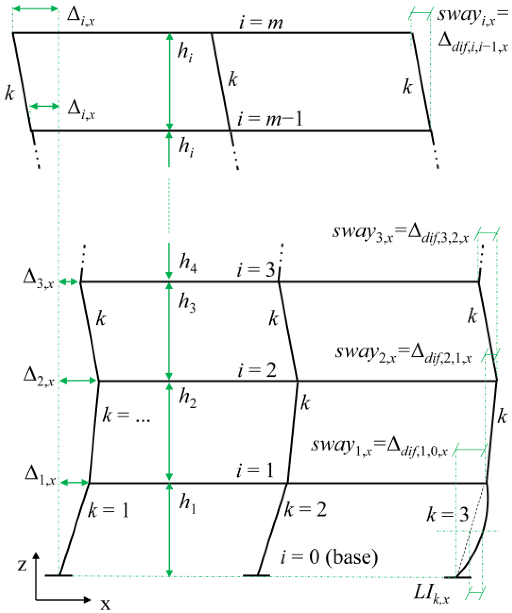
2.2.1. #RSS Method (Random Storey Sway)

The first approach is to consider the random input of sways for each storey, based on Equation (2). The sways are considered as angles of declination from the vertical direction, and the mean value of each storey sway would be 0, with the standard deviation of 1/600 radians.

In this approach, it appears to be useful to conduct a verification using the criterion of the Equation (1), and thus to check the number of random realizations that violate the maximal value of storey deviation relative to the base position, verified for each storey separately. Ideally, there should be approximately 5% of these violations for each corresponding storey.

This approach is further noted as the “random storey sways” method, or #RSS, as the stochastic inputs are the sways of each i-th storey (sway_i, or shorter notation sw_i). A certain limit for the location of each storey relative to the base position (the criterion of Equation (1) to be verified) is already partially indirectly incorporated in the logic of what is considered as the random parameters for input due to the fact that the geometry of each storey is bonded to the position of the storey below. It is questionable whether, for greater numbers of storeys, the number of random realizations that would violate the criteria for the locations of the uppermost stories relative to the base would still be approximately 5%, and what the influence would be on the structural resistance determined by statistical methods.

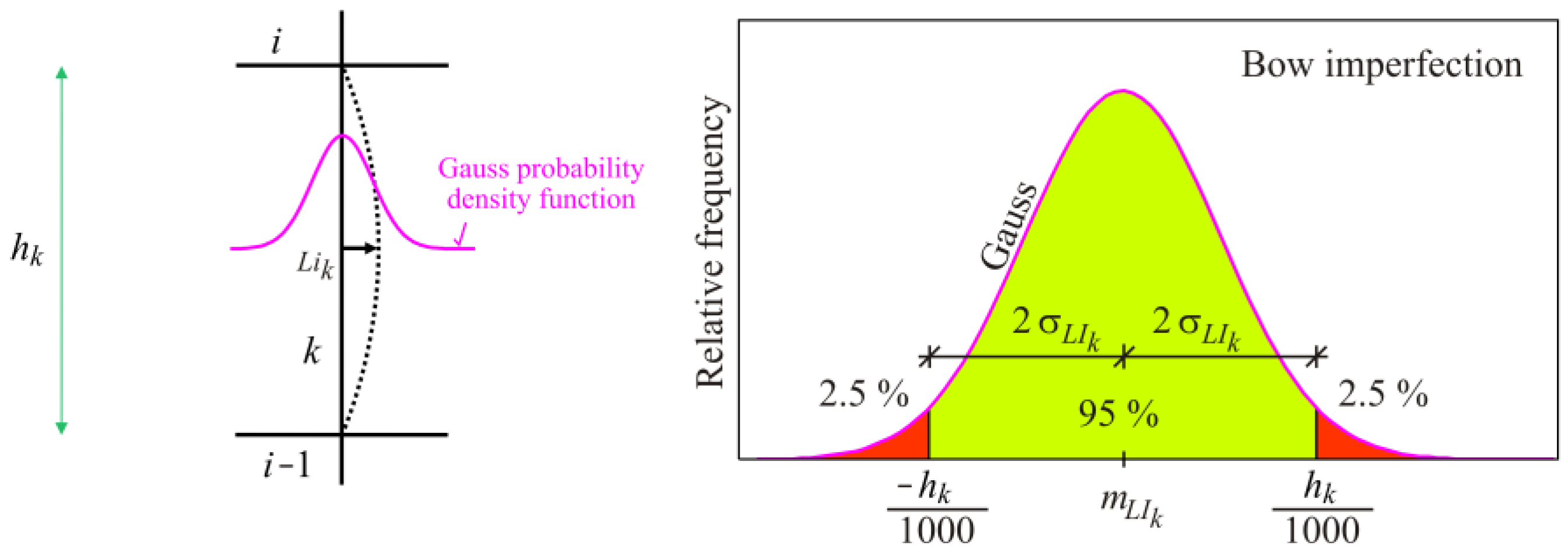
2.2.2. #RSP Method (Random Storey Positions)

The second approach would be to consider the mean values of each i-th storey deviation relative to the position of the base Δ_i (Figure 1) as 0 mm, and the standard deviations would be derived for each storey based on Equation (1). Hence, different standard deviations are given for each i-th storey, and larger values are yielded with increasing levels of the corresponding storey.

Subsequently, the maximal mutual deviations of each set of two adjacent storeys (sways) needs to be verified—Equation (2)—as does whether a maximum of 5% of random realizations are violating the considered criterion. In this case, certain correlations (positive) between the input Δ_i parameters (storey deviations relative to the base position) need to be introduced, mainly for multiple storey structures. Otherwise, this approach would lack any relation between two adjacent storeys, resulting in too many realizations violating the tolerance criteria for storey sways (Equation (2)).

This approach will be further noted as the “random storey position” method (approach #RSP), as the inputs are deviations relative to the base position Δ_i (Figure 1). The question is, what values of the mutual correlations should be used.

3. Verifications of the Stochastic Methods of #RSS and #RSP

In both approaches, the Advanced Latin Hypercube Sampling (ALHS) method has been used to generate the random realizations. In this method, the correlation errors are minimized by the stochastic evolution strategies [42]. The representation of the specified input distributions and the input correlations is also very accurate when the standard Latin Hypercube Sampling (LHS) method [43] is used, whereby a method to minimize the undesired correlations is implemented (Iman and Conover) [44]. Furthermore, it is easier to work with sampling methods when there is a correlation between parameters, e.g., [45,46,47]. ALHS has been preferred, as it is recommended for not so large numbers of input parameters [48]. To manage ALHS sampling, the OptiSLang version 7.4.1 software [48] has been used.

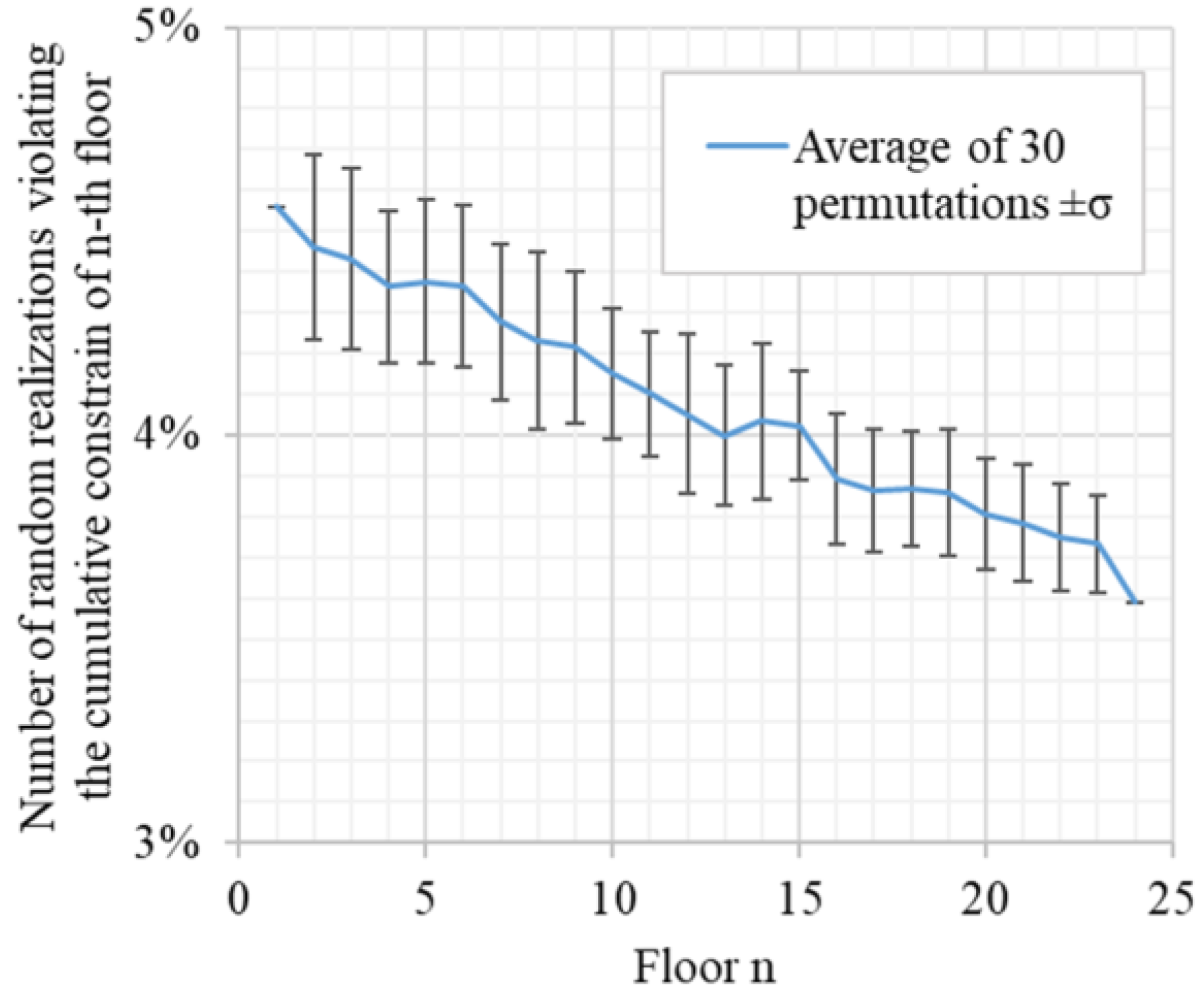
3.1. Random Storey Sway (#RSS) Method Verification

In order to verify the number of violated tolerances for each floor, a 24-storey structure is considered, with an equidistant storey height of h (h was considered as 4.5 m for the verification, but the value itself does not matter as long as the storeys are equidistant). Here, 10,000 random realizations of sways are generated for set of 24 storeys (sets noted as A, B, C, … X), with the mean value of 0 and standard deviation of 1/600 radians for each storey. The standard Gauss distribution is considered. Each storey-set (A, B, C, … X) of 10,000 random sway realizations then might be considered as a set of random sways of any storey number (1, 2, 3, … 24), hence 30 random permutations (I., II., III., … XXX.) of the storey-set to storey number assignments have been considered (the order of random realizations within the 10,000 random realizations of each set A, B, C, … X is kept). Examples of 3 of these 30 permutation assignments are depicted in a matrix in

Table 1. Example of the permutation assignments.

Assigned Permutation	Storey-Set
	A	B	C	D	E	F	G	H	I	J	K	L	M	N	O	P	Q	R	S	T	U	V	W	X
I.	1	2	3	4	5	6	7	8	9	10	11	12	13	14	15	16	17	18	19	20	21	22	23	24
II.	15	8	13	23	19	24	20	9	12	10	4	18	21	2	1	22	5	7	6	3	14	17	16	11
III.	6	21	1	11	9	10	24	16	22	3	19	18	4	13	8	14	15	5	17	2	7	20	23	12

. For example, the I. permutation considers all the 10,000 random sways of set A as sways of the first floor, sways of the set B as sways of the second floor, etc. All the other permutations (II.–XXX.) are then randomly mixed, e.g., in permutation II., the set of random sways A is considered as random sways of the 15th floor. This approach has been used in order to reduce the amount of data used for statistical post-processing (instead of 30 × 24 sets of 10,000 random realizations, only 24 such sets have been created).

For each set of 30 random permutations, the cumulative deviations Δ_i of each i storey relative to the position of the base are expressed, and compared with the maximal permitted deviation (Equation (1)). The relative numbers of random realizations that violate these cumulative tolerances are monitored for each storey, and the average values along with standard deviation bars (of the 30 permutations) are depicted in Figure 3.

Note: For the 1st and last (24th) floors, these values are the same (4.56% and 3.59%, respectively) in all 30 permutations, hence the 0 standard deviation. The reason in the case of the first floor is the fact the storey deviation depends only on the sway of the first floor itself (Equation (1) is the same as Equation (2) for i = 1). For each storey sway, the 2 sigma rule has been considered in order to achieve 5% of the random realization violating the tolerance (Equation (2)). This value for the ALHS algorithm is precisely 4.56% (not exactly 5%), as the number 2 within the 2 sigma rule is rounded. For all the sets (A, B, C, … X), the relative number of realizations violating the tolerance of maximal inclination (Equation (2)) is the same, hence, it does not matter which of the 24 sets is to be considered as the set for the 1st floor. The value for the last (24th) floor is the same for all 30 permutations, as the final deviation of this last floor relative to the base does not depend on the order of individual sways (for equidistant floors).

In general, the number of random realizations violating the cumulative tolerance (Equation (1)) decreases with the increasing storey number (Figure 3). The decrease appears to be approximately linear, on average −0.0375% per storey. Approximately up to the 15th floor, the number of these realizations violating the cumulative tolerance is still around 4%. For the 23rd floor, the average number is 3.73%. In order to get a more precise value for the 24th floor, either additional random realizations of 24 sway parameters would be necessary, or permutations of sway assignments for larger floor numbers are required. This has not been further investigated in detail, as the objective, the decreasing trend and its intensity, has been found already.

Overall, it appears this approach, #RSS, might be used without any additional modification for smaller numbers of floors. For larger numbers of storeys, it is questionable whether the number of realizations that violate the cumulative tolerances for the uppermost floors is not too small, as the value is not as close to the 5% threshold.

3.2. Random Storey Position (#RSP) Method Verification

Similarly to the previous verification, 24 floor structures are here considered, with an equidistant storey height h of 4.5 m. The random inputs are storey deviations relative to the position of the base. For each storey, the mean value of this deviation is set to 0 mm, and the standard deviation σ_Δj is set in accordance with

Table 2. Example of the standard deviations for the random input of storey positions relative to the base.

Storey Number i	Σhj (m)	σΔj (mm)	Storey Number i	Σhj (m)	σΔj (mm)
1	4.5	7.500	13	58.5	27.042
2	9.0	10.607	14	63.0	28.062
3	13.5	12.990	15	67.5	29.047
4	18.0	15.000	16	72.0	30.000
5	22.5	16.771	17	76.5	30.923
6	27.0	18.371	18	81.0	31.820
7	31.5	19.843	19	85.5	32.692
8	36.0	21.213	20	90.0	33.541
9	40.5	22.500	21	94.5	34.369
10	45.0	23.717	22	99.0	35.178
11	49.5	24.875	23	103.5	35.969
12	54.0	25.981	24	108.0	36.742

, where the values are derived from the tolerance Equation (1) considering the 2 sigma rule.

Additionally, these storey deviations are mutually correlated through the Gaussian correlation function (Equation (4)), which represents a 1D random field with correlation length L_cor (m) and was used also in [49]:

$${\rho }_{jh}=p\cdot e^{-{({\zeta }_{jh}/L_{cor})}^2},$$

(4)

where ρ_jh is the member of the correlation matrix, p is the multiplication factor set to ensure the matrix is definitely positive (applicable mainly for larger matrixes, considered as 0.99, except for diagonal matrix members that are exactly 1.0), and ζ_jh is the vertical distance between two points (two floors). Various correlation lengths L_cor are verified.

In this approach, the maximal deviations of each set of two adjacent storeys needs to be verified—Equation (2)—as does whether a maximum of 5% of random realizations are violating the considered criterion. Hence, it is necessary to find the smallest possible value of the correlation length L_cor, such that the number of random realizations that violate this tolerance (Equation (2)) is below 5% for each pair of two adjacent storeys of an m-storey structure with equidistantly spaced floors (each with a height of h).

These optimal values of correlation lengths L_cor are to be determined for 2–24-storey structures, expressed relatively as the ω ratio, which is a function of m:

$$\omega (m)=\frac{L_{cor}}{m\cdot h},$$

(5)

where m is the total number of floors, each with a height of h. As long as the vertical distance between two floors ζ_jh might be expressed as a natural multiplication n·h of the storey height h, Equation (4) can be expressed as:

$${\rho }_{jh}=p\cdot e^{-{\left(\frac{n}{\omega (m)\cdot m}\right)}^2},$$

(6)

where n is the relative distance between two floors (e.g., n = 1 for the distance between the first floor and the second floor). The values of ω ratio are determined considering the storey height h = 4.5 m, with corresponding values of the L_cor.

Firstly, for the 24-floor structure, nine different values of the correlation lengths L_cor have been verified (13.5, 18.0, 22.5, 27.0, 31.5, 36.0, 40.5, 45.0 and 54.0 m) in order to determine the correlation matrixes (Equation (4)). For each of these nine sets, 10,000 random realizations of the 24 input parameters (24 random storey deviations relative to the position of the base Δ_i) have been generated by the ALHS method. For each of these nine sets, the number of realizations that violate the maximal column inclination between two adjacent floors (Equation (2)) is monitored for each pair of two adjacent floors. For easier notation, this inclination between ith and i − 1st floor is noted as the sway of the ith floor (e.g., the sway of the third floor is determined from the inclination of the columns between the second and third floor levels; see Figure 1, sway_i = Δ_dif,i,i−1). This workflow is graphically depicted in Figure 4.

Afterwards, in order to determine the optimal correlation length L_cor for each ith floor more precisely and to verify this value, several more sets using linearly interpolated values of the L_cor have been realized. This time, for the determination of the optimal L_cor for the ith storey, only an i-storey structure was considered (with i random storey deviations) to decrease unnecessary data. However, to be more precise, for each of these interpolated L_cor values, the ratio of random realizations that violate the maximal sway of the corresponding floor (Equation (2)) is determined as the average of four sets, each with 10,000 random realizations. For each floor, the L_cor values are determined more precisely until the ratio of random realizations that violate the sway tolerance is 5% ± 0.2%. If the ratio fits within this tolerance, L_cor is considered as optimal for the corresponding ith floor.

These values of the correlation lengths L_cor for structures up to 24 floors (floor heights h = 4.5 m) and the corresponding ratio of realizations violating the sway of the corresponding ith floor number (sway_i = Δ_dif,i,i−1) are graphically depicted in Figure 5.

In this graph, the dots represent relative numbers of random realizations that violate the sways tolerances either for 10,000 random realizations (those dots where L_cor = 13.5, 18.0, 22.5, 27.0, 31.5, 36.0, 40.5, 45.0 and 54.0 m) or based on an average of four sets, each comprising 10,000 random realizations (the more exact values are based on the interpolated L_cor values). Note: For the fourth and third floors, the optimal L_cor value is verified based on an average of 10 sets (each with 10,000 random realizations), and for the second floor the average is made of two sets of 10,000 random realizations. It was found that using 10 sets does not improve the precision significantly compared to four sets. On the other hand, using two sets seems to be feasible, but four sets are more precise, hence this number was used for all the other floors.

The optimal values of the correlation lengths L_cor for a structure of storey height h = 4.5 m, and the relatively expressed ω ratio (independent of the storey height h), are summarized in

Table 3. Summary of the optimal correlation values L_cor expressed relatively by the ω ratio.

m-Storey Structure	Lcor (m) (for h = 4.5 m)	ω(m) (-)	m-Storey Structure	Lcor (m) (for h = 4.5 m)	ω(m) (-)
1	-	-	13	25.60	0.4376
2	7.50	0.8333	14	26.60	0.4222
3	9.80	0.7259	15	27.90	0.4133
4	11.70	0.6500	16	29.50	0.4097
5	13.72	0.6098	17	30.35	0.3967
6	15.51	0.5744	18	31.93	0.3942
7	17.06	0.5416	19	33.80	0.3953
8	18.46	0.5128	20	35.00	0.3889
9	19.73	0.4872	21	36.56	0.3869
10	21.44	0.4764	22	38.00	0.3838
11	22.34	0.4513	23	39.80	0.3845
12	24.00	0.4444	24	42.20	0.3815

.

Graphically, the ω ratio is depicted in Figure 6a, and it appears that linear approximation of the ratio ω is feasible for floors 17–24, or for the extrapolation of higher storeys; see Figure 6b.

In this #RSP approach, the ratios of random realizations violating the maximal sway tolerances for the i−1, i−2, … second floor in the case of an i-storey structure are significantly below 5% if the optimal L_cor (or relative ω ratio) for the ith storey is considered. For example, in the case of a seven-storey structure, the optimal correlation length for the storey height h = 4.5 m is L_cor = 17.06 m (Table 3), but for this value, the percentages of realizations violating the sway tolerances for the sixth, fifth, fourth, third and second floor are 3.42%, 2.13%, 1.06%, 0.41% and 0.08%, respectively (see Figure 5, the dots at L_cor = 17.06 m). Note: The first floor is not depicted in the graph, as the sway of the first floor is dependent only on the directly input value of the cumulative tolerance Δ₁ for the first floor (the storey deviation relative to the position of the base)—see Figure 1, where Δ₁ = sway_i = Δ_dif,I,i−1. Hence, the number of realizations that violate the sway tolerance of the first floor is the same as the number of realizations that violate the cumulative tolerance for the first floor, and this value is approximately 4.4%, independent of the considered L_cor value, as will be further discussed (Figure 7).

Furthermore, the numbers of random realizations that violate the cumulative tolerance (Equation (1)), and thus the direct input of storey deviations relative to the base position, are verified (as there are correlations between these inputs). These values have been monitored and averaged for each storey in nine sets of 24-storey structures (with L_cor values of 13.5, 18.0, 22.5, 27.0, 31.5, 36.0, 40.5, 45.0 and 54.0 m), and the values along with their standard deviations are depicted in Figure 7a. In this graph, each dot represents an average value for nine sets, where each set contains 10,000 random realizations. Due to input correlations between the parameters, the utilized ALHS algorithm generates slightly different numbers of realizations that violate the cumulative tolerance for each floor. It appears that there is some local minimum in this value in the mid-part of the floor, with the averaged value of 4.3% for the 1st and 24th floor, and around 4.0% near the 12th floor. In general, the mid-floor values are more correlated (to both sides, up and down), and on the other hand, the edge floors are correlated only to one side. Otherwises the deviations of these values are not so large.

The standard deviations of the graph in Figure 7a are slightly scattered, hence the same was verified for all the realizations used to determine the optimal L_cor values more precisely (in short, “all the dots” from Figure 5, except those already used for the graph in Figure 7a). The result is presented in Figure 7b. When averaging from a larger data set, a similar tendency is observed, with slightly more aligned standard deviations. It is important to note that in the case of this graph (Figure 7b), the data set is different for each floor. The reason is that this graph was created from data used to determine more precise L_cor values for various storey structures. As was mentioned before, in order to more precisely determine L_cor for the n-th storey, only the n-storey structure was considered. But an n-storey structure also contains data for the n − first, n − second, … first floors. Hence, since these data were already available, they have also been used for the averaging. The data that were used to build the graph in Figure 7b are depicted in Figure 8. For example, for the 24th floor, there are 8 × 10,000 random realizations. This correlates with the two additional points for the 24th floor line shown in Figure 5 (where each point is an average of 4 sets of 10,000 realizations). The largest data set is apparently related to the first floor, as all of the n-storey structures contain the first floor.

The numbers of random realizations that violate the cumulative tolerance have also been verified via a different averaging approach. This time, the averaging was done using the data set of all the floors, separately, for each n-storey structure. The averaged values are depicted in Figure 9, and the data set out of which the values were averaged is in Figure 10. For example, there were two sets of 10,000 random realizations of two-storey structures, hence the combined data were averaged out of four floors for the two-storey structure. There were two 24-storey structures (with L_cor = 41.2 and 41.6 m—see Figure 5), and each contained four sets of 10,000 random realizations, hence for the 24-storey structure, the average was composed of 2 × 4 × 24 = 192 floors together. Although the data set differs for each n-storey structure, the number of realizations that violate the cumulative tolerance (of any floor of the considered structure) seems to slightly decrease with the increasing number of floors of the structure (Figure 9). This decrease is in general not so large.

Overall, the number of random realizations that violate some cumulative tolerance (considering the 2 sigma rule) is approximately 4.3% for any floor of any of the n-th-storey structures in the considered data set. This seems reasonable, and is not so far from the 5% threshold. However, in this #RSP approach, the previously discussed number of realizations that violate the sway tolerance appears to be more questionable (Figure 5).

4. Discussion of the #RSS and #RSP Approaches

The input statistical parameters based on the tolerance criteria in accordance with Table B.18 of Annex B of standard EN 1090-2:2018 [11] are considered in both the approaches, #RSS and #RSP. For the #RSS (random storey sway), the random inputs are based on Equation (2) and the tolerances derived from Equation (1) are verified. For the #RSP approach (random storey position), the input parameters are derived from Equation (1), and Equation (2) is used for the verification. In general, both approaches are correct.

The advantage of the #RSS approach is that the input parameters (random storey sways) have zero mutual correlations. The number of random realizations violating any sway tolerance is equal to 4.56% (when the 2 sigma rule is considered to determine the standard deviation from the tolerance criterion), which is close to 5% and the same for all uncorrelated random inputs. The verification of the cumulative tolerances (Equation (1)) resulted in ratios of violations between 5% and 4% for the 1st to about the 15th floor (Figure 4). This ratio decreases for higher floors, and might have some impact on the structural resistance determined by statistical methods (e.g., first-order reliability method—FORM), depending also on the load distribution of such structures.

On the other hand, the #RSP approach requires the definition of mutual correlations between the input parameters (storey deviations relative to base), making it less robust for utilization. Therefore, optimal correlations for structures up to 24 storeys expressed relatively as ω ratios (which might be used for a structure with any number of (equidistantly placed) storeys of height h) have been determined (Figure 6a, Table 3). Due to the correlated inputs, the numbers of random realizations that violate the cumulative tolerances are not the same, but are slightly variable (see averages in the Figure 7a,b and Figure 9), and are in general around 4.3%, which might be considered as acceptable. However, in order to achieve the 5% of random realizations that violate the sway tolerance of the last, ith floor, the number of realizations that violate the tolerances of the other floors must be much smaller than 5% (Figure 5). It is unknown what the impact would be on the structural resistance.

The provisions offered by this paper include the optimal correlation lengths (Table 3), which might be used in further numerical analyses of steel frame structures via the utilization of finite element methods. For example, the #RSS method, as presented here, has been used, along with the probabilistic FORM method [28], for stochastic analyses of a three-storey steel frame, as has been presented in a previous verification study [38]. In this study, the ultimate resistance of a steel frame structure was compared, in accordance with the FORM method, with the resistance of a deterministic design, in accordance with the assumptions of the EN standard for steel structure design [20]. However, this verification was conducted based only on one specific type of steel frame geometry. In future research, the ultimate resistances of several different steel frame geometries will be estimated via the stochastic FORM approach [28] and compared with the assumptions in the EN standard [20]. The resistances will be estimated using both methods verified in this paper, #RSS and #RSP, along with the FORM method, in order to investigate the influences of these presented methods on the structural resistance of steel frame structures. In other studies, models based on the correlation length have been utilized to enhance the understanding of imperfections arising in bridge arch analyses [50] and the seismic resistance of steel-braced frames [12].

5. Conclusions

This study introduces two distinct methods, namely, the random storey sway (#RSS) and the random storey position (#RSP), in order to incorporate stochastic parameters associated with the global geometrical imperfections of steel frame structures. The #RSS method focuses on rotations caused by column out-of-verticality between different floors (storey sways), while the #RSP method focuses on floor positions relative to the base. The #RSS method stands out by eliminating the need for incorporating correlations between statistical parameters related to member rotations among floors. Conversely, the #RSP method requires the utilization of correlations between the deviations of individual floors, defined by a random field, and approaches to defining the optimal correlations are provided in this study.

Both of these methods have been tested on structures with up to 24 floors using numerous randomly generated input parameter values. It might be concluded that the utilization of both method is feasible, with possible limitations in the #RSS when applied to structures with more storeys (above 24). The #RSP method is limited to the defined correlation values, which are provided for structures of up to 24 floors. It is expected that the structural resistances given by the #RSP and #RSS methods will differ for structures of more storeys. This needs to be verified in future research via numerical analyses of several steel-framed structures with various geometries.

Both of the presented methods, #RSS and #RSP, offer ways to consider statistical input parameters (storey sways or storey positions) as part of a probabilistic method to directly model the initial geometrical imperfections of steel frames (via changes in the model’s geometry). The proposed methods might be utilized in 3D numerical analyses of steel structures. The probabilistic method used to directly model the initial geometrical imperfections offers more accurate representations of real-world structural geometries compared with other methods, such as the scaling of the elastic buckling modes (EBM), the notional horizontal forces method (NHF), or member stiffness reduction. The statistical values (mean value and standard deviation) of the input parameters (sways or positions) for the #RSS and #RSP methods are derived from the tolerance criteria set in the standard for the building of steel structures, and these values are similar to those measured in real structures. Hence, the values might be considered as rather realistic, and not overly conservative. The presented probabilistic methods might also be feasibly used to verify all the other deterministic approaches applied to model initial geometrical imperfections (in various frame geometries), without conducting a costly physical experiment on such a structure.

References

1. Melcher, J. Classification of structural steel members initial imperfections. In Structural Stability Research Council: Proceedings 1980; Lehigh University: Bethlehem, PA, USA, 1980; Available online: https://scholarsmine.mst.edu/ccfss-library/234 (accessed on 12 August 2023).
2. Kala, Z. Sensitivity assessment of steel members under compression. Eng. Struct. 2009, 31, 1344–1348. [Google Scholar] [CrossRef]
3. Chen, G.; Zhang, H.; Rasmussen, K.J.; Fan, F. Modeling geometric imperfections for reticulated shell structures using random field theory. Eng. Struct. 2016, 126, 481–489. [Google Scholar] [CrossRef]
4. Wang, J.; Li, H.-N.; Fu, X.; Li, Q. Geometric imperfections and ultimate capacity analysis of a steel lattice transmission tower. J. Constr. Steel Res. 2021, 183, 106734. [Google Scholar] [CrossRef]
5. Jůza, J.; Jandera, M. I-section stainless steel portal frames: Loading tests and numerical modelling. J. Constr. Steel Res. 2024, 212, 108293. [Google Scholar] [CrossRef]
6. Ma, T.; Xu, L. Effects of column imperfections on capacity of steel frames in variable loading. J. Constr. Steel Res. 2020, 165, 105819. [Google Scholar] [CrossRef]
7. Dario Aristizabal-Ochoa, J. Second-order slope–deflection equations for imperfect beam–column structures with semi-rigid connections. Eng. Struct. 2010, 32, 2440–2454. [Google Scholar] [CrossRef]
8. Nowak, A.S.; Collins, K.R. Reliability of Structures; McGraw-Hill: New York, NY, USA, 2000; Available online: https://www.researchgate.net/publication/37427378_Reliability_of_Structures (accessed on 10 October 2023).
9. Liu, W.; Rasmussen, K.J.R.; Zhang, H. Systems reliability for 3D steel frames subject to gravity loads. Structures 2016, 8, 170–182. [Google Scholar] [CrossRef]
10. Liu, W. System Reliability-Based Design of Three-Dimensional Steel Structures by Advanced Analysis. Ph.D. Thesis, The University of Sydney, Sydney, Australia, 2016. Available online: https://ses.library.usyd.edu.au/handle/2123/16126 (accessed on 10 December 2023).
11. BS EN 1090-2:2018; Execution of Steel Structures and Aluminium Structures Part 2: Technical Requirements for Steel Structures. British Standard Institution (BSI): London, UK, 2018.
12. Jin, T.; Yu, H.; Li, J.; Hao, G.; Li, Z. Design and seismic performance of tied braced frames. Buildings 2023, 13, 1652. [Google Scholar] [CrossRef]
13. Antonodimitraki, S.; Thanopoulos, P.; Vayas, I. EC3-compatible methods for analysis and design of steel framed structures. Modelling 2021, 2, 567–590. [Google Scholar] [CrossRef]
14. Chacón, R.; Puig-Polo, C.; Real, E. TLS measurements of initial imperfections of steel frames for structural analysis within BIM-enabled platforms. Autom. Constr. 2021, 125, 103648. [Google Scholar] [CrossRef]
15. Baláž, I.; Koleková, Y.; Agüero, A.; Balážová, P. Consistency of imperfections in steel Eurocodes. Appl. Sci. 2023, 13, 554. [Google Scholar] [CrossRef]
16. Zhang, Z.-J.; Chen, B.-S.; Bai, R.; Liu, Y.-P. Non-Linear Behavior and Design of Steel Structures: Review and Outlook. Buildings 2023, 13, 2111. [Google Scholar] [CrossRef]
17. Shayan, S.; Rasmussen, K.J.R.; Zhang, H. On the modelling of initial geometric imperfections of steel frames in advanced analysis. J. Constr. Steel Res. 2014, 98, 167–177. [Google Scholar] [CrossRef]
18. Gu, J.X.; Chan, S.L. Second-order analysis and design of steel structures allowing for member and frame imperfections. Int. J. Numer. Methods Eng. 2005, 62, 601–615. [Google Scholar] [CrossRef]
19. Kala, Z. Strain energy and entropy based scaling of buckling modes. Entropy 2023, 25, 1630. [Google Scholar] [CrossRef]
20. EN 1993-1-1:2005+A1:2014; Eurocode 3: Design of Steel Structures Part 1-1: General Rules and Rules for Buildings. European Committee for Standardization: Brussels, Belgium, 2014.
21. Kim, S.E. Practical Advanced Analysis for Steel Frame Design. Ph.D. Thesis, Purdue University, West Lafayette, IN, USA, 1996. Available online: https://docs.lib.purdue.edu/dissertations/AAI9638189/ (accessed on 5 November 2023).
22. Chan, S.L.; Huang, H.Y.; Fang, L.X. Advanced analysis of imperfect portal frames with semirigid base connections. J. Eng. Mech. 2005, 131, 633–640. [Google Scholar] [CrossRef]
23. AISC 360; Specification for Structural Steel Buildings. American Institute of Steel Construction: Chicago, IL, USA, 2016.
24. Bernuzzi, C.; Cordova, B.; Simoncelli, M. Unbraced steel frame design according to EC3 and AISC provisions. J. Constr. Steel Res. 2015, 114, 157–177. [Google Scholar] [CrossRef]
25. Bažant, Z.P.; Xiang, Y. Postcritical imperfection-sensitive buckling and optimal bracing of large regular frames. J. Struct. Eng. 1997, 123, 513–522. [Google Scholar] [CrossRef]
26. Agüero, A.; Baláž, I.; Koleková, Y.; Martin, P. Assessment of in-Plane Behavior of Metal Compressed Members with Equivalent Geometrical Imperfection. Appl. Sci. 2020, 10, 8174. [Google Scholar] [CrossRef]
27. Liew, J.Y.R.; White, D.W.; Chen, W.F. Notional-load plastic-hinge method for frame design. J. Struct. Eng. 1994, 120, 1434–1454. [Google Scholar] [CrossRef]
28. EN 1990:2002; Eurocode—Basis of Structural Design. European Committee for Standardization: Brussels, Belgium, 2002.
29. De Domenico, D.; Falsone, G.; Settineri, D. Probabilistic buckling analysis of beam-column elements with geometric imperfections and various boundary conditions. Meccanica 2018, 53, 1001–1013. [Google Scholar] [CrossRef]
30. Chepurnenko, A.; Turina, V.; Akopyan, V. Simplified method for calculating the bearing capacity of slender concrete-filled steel tubular columns. CivilEng 2023, 4, 1000–1015. [Google Scholar] [CrossRef]
31. Quan, C.Y.; Walport, F.; Gardner, L. Equivalent imperfections for the out-of-plane stability design of steel beams by second-order inelastic analysis. Eng. Struct. 2021, 251, 113481. [Google Scholar] [CrossRef]
32. Kala, Z.; Valeš, J. Sensitivity assessment and lateral-torsional buckling design of I-beams using solid finite elements. J. Constr. Steel Res. 2017, 139, 110–122. [Google Scholar] [CrossRef]
33. Zhang, H.; Shayan, S.; Rasmussen, K.J.R.; Ellingwood, B.R. System-based design of planar steel frames, I: Reliability framework. J. Constr. Steel Res. 2016, 123, 135–143. [Google Scholar] [CrossRef]
34. Liu, W.; Rasmussen, K.J.R.; Zhang, H.; Xie, Y.; Liu, Q.; Dai, L. Probabilistic study and numerical modelling of initial geometric imperfections for 3D steel frames in advanced structural analysis. Structures 2023, 57, 105190. [Google Scholar] [CrossRef]
35. Lindner, J.; Gietzelt, R. Imperfektionsannahmen für Stützenschiefstellungen (Assumptions for imperfections for out-of-plumb of columns). Stahlbau 1984, 53, 97–102. [Google Scholar]
36. Prokop, J.; Vičan, J.; Jošt, J. Numerical analysis of the beam-column resistance compared to methods by European standards. Appl. Sci. 2021, 11, 3269. [Google Scholar] [CrossRef]
37. Jönsson, J.; Stan, T.C. European column buckling curves and finite element modelling including high strength steels. J. Constr. Steel Res. 2017, 128, 136–151. [Google Scholar] [CrossRef]
38. Jindra, D.; Kala, Z.; Kala, J. Ultimate Load Capacity of Multi-Story Steel Frame Structures with Geometrical Imperfections: A Comparative Study of Two Methods. In Modern Building Materials, Structures and Techniques. MBMST 2023; Lecture Notes in Civil Engineering; Springer: Cham, Switzerland, 2023; Volume 392. [Google Scholar] [CrossRef]
39. Kalogeris, I.; Papadopoulos, V. Limit analysis of stochastic structures in the framework of the Probability Density Evolution Method. Eng. Struct. 2018, 160, 304–313. [Google Scholar] [CrossRef]
40. Schillinger, D.; Papadopoulos, V.; Bischoff, M.; Papadrakakis, M. Buckling analysis of imperfect I-section beam-columns with stochastic shell finite elements. Comput. Mech. 2010, 46, 495–510. [Google Scholar] [CrossRef]
41. Radwan, M.; Kövesdi, B. Equivalent geometric imperfection for interaction buckling of welded box-section columns—Stochastic analysis. J. Constr. Steel Res. 2024, 213, 108374. [Google Scholar] [CrossRef]
42. Hungtington, D.E.; Lyrintzis, C.S. Improvements to and limitations of Latin hypercube sampling. Probabilistic Eng. Mech. 1998, 13, 245–253. [Google Scholar] [CrossRef]
43. McKay, M.D.; Beckman, R.; Conover, W. A comparison of three methods for selecting values of input variables in the analysis of output from a computer code. Technometrics 1979, 21, 239–245. [Google Scholar] [CrossRef]
44. Iman, R.L.; Conover, W.J. A distribution-free approach to inducing rank correlation among input variables. Commun. Stat. Simul. Comput. 1982, 11, 311–334. [Google Scholar] [CrossRef]
45. Mahmood, A.; Varabuntoonvit, V.; Mungkalasiri, J.; Silalertruksa, T.; Gheewala, S.H. A Tier-wise method for evaluating uncertainty in life cycle assessment. Sustainability 2022, 14, 13400. [Google Scholar] [CrossRef]
46. Xie, M.; Yuan, J.; Jia, H.; Yang, Y.; Huang, S.; Sun, B. Probabilistic seismic sensitivity analyses of high-speed railway extradosed cable-stayed bridges. Appl. Sci. 2023, 13, 7036. [Google Scholar] [CrossRef]
47. Magini, R.; Moretti, M.; Boniforti, M.A.; Guercio, R. A Machine-learning approach for monitoring water distribution networks (WDNs). Sustainability 2023, 15, 2981. [Google Scholar] [CrossRef]
48. Dynardo GmbH, OptiSLang Software Manual: Methods for Multi-Disciplinary Optimization and Robustness Analysis, Weimar. 2019. Available online: https://www.ansys.com/products/platform/ansys-optislang (accessed on 7 September 2023).
49. Kala, Z.; Valeš, J.; Jönsson, J. Random fields of initial out of straightness leading to column buckling. J. Civ. Eng. Manag. 2017, 23, 902–913. [Google Scholar] [CrossRef]
50. Odrobiňák, J.; Farbák, M.; Chromčák, J.; Kortiš, J.; Gocál, J. Real geometrical imperfection of bow-string arches—Measurement and global analysis. Appl. Sci. 2020, 10, 4530. [Google Scholar] [CrossRef]
Figure 1. Tolerance criteria for the steel frame structures.
Buildings 14 00196 g001
Figure 2. Stochastic model of initial bow imperfections.
Buildings 14 00196 g002
Figure 3. Verification of the cumulative tolerance criterion for the #RSS method.
Buildings 14 00196 g003
Figure 4. Workflow used to determine the optimal values of the correlation lengths for each floor.
Buildings 14 00196 g004
Figure 5. Verification of the storey sway tolerance criterion for the #RSP method.
Buildings 14 00196 g005
Figure 6. The values of the ω ratio: (a) Optimal values of the ω ratio used to determine the optimal correlation length for the #RSP method; (b) linear approximation of the optimal ω ratio for a 17–24-storey structure.
Buildings 14 00196 g006
Figure 7. Ratio of random realizations violating the maximal cumulative tolerance of the corresponding n-th floor: (a) Selected sets; (b) average.
Buildings 14 00196 g007
Figure 8. Data set for averaging (for graph in Figure 7b).
Buildings 14 00196 g008
Figure 9. Ratio of random realizations violating the maximal cumulative tolerance for all the floors of n-th storey structure.
Buildings 14 00196 g009
Figure 10. Amount of data used for averaging (for graph in the Figure 9).
Buildings 14 00196 g010