Abstract
The objective of this paper is to show a study on the influence of vegetation on the outdoor thermal comfort (OTC) of a high-altitude tropical megacity. The OTC is evaluated by the PET (Physiological Equivalent Temperature) index and by establishing three simulation scenarios: (i) Current OTC, (ii) OTC under RCPs 4.5 and 8.5 (Representative Concentration Pathway), and (iii) OTC under RCPs and ENSO (El Niño–Southern Oscillation). The results show that the hourly variation range of the current OTC in urban areas with vegetation is greater (+3.15 °C) compared to impermeable areas. Outdoor thermal stress due to cold in vegetated areas is 1.29 °C lower compared to impervious areas. The effect of vegetated coverage on the improvement of urban OTC increases as the phenomenon of global warming intensifies. On average, in the current, RCP4.5, and RCP8.5 scenarios for each 10% increase in urban vegetation coverage, an increase of 0.22, 0.24, and 0.28 °C in OTC is obtained, respectively. The hourly variation range of the PET index increases during the ENSO scenario (vegetated areas: +16.7%; impervious areas: +22.7%). In the context of climate change and variability, this study provides a reference point for decision-makers to assess possible planning options for improving OTC in megacities.
1. Introduction
Worldwide, it was estimated that since pre-industrial times the temperature of the planet increased by approximately 1.0 °C and that this increase was progressive during the 21st century [1]. The increase in temperature associated with climate change could contribute to the occurrence of warmer days, mainly in low latitude areas, and in the manifestation of more heat waves, with greater incidence in cities [2,3]. This environmental problem has also been intensified in cities because urban growth was one of the main causes of natural ecosystem degradation and therefore of decrease in outdoor thermal comfort (OTC) [4]. The previous urban trend also increased the loss of environmental quality and well-being of the inhabitants [5]. Thus, the accelerated growth, reduction of natural areas, and low percentage of vegetated areas were aspects of concern in relation to the temperature increase in urban areas [6].
The effects of temperature increase in urban areas were also intensified due to the increase in energy demand from cooling systems, CO2 emission by electric power plants, and emissions from the use of fossil fuels and refrigerant gases in air conditioners and refrigerators [7,8]. Urban adaptation strategies to the possible impacts of climate change included increased vegetation, use of cold roofs that could be vegetated or with greater solar reflectance, and increasing cold pavements [9,10]. Therefore, it is necessary to develop studies on the influence of vegetation on OTC in urban areas. These types of studies will be useful for decision-makers in public and private institutions, who are continually looking for tools to guide the planning of their cities. The increase in temperature is one of the planning challenges that cities must continue to address in the coming years, as well as its possible intensification due to phenomena such as El Niño—Southern Oscillation (ENSO) and heat islands.
In the IPCC’s Fifth Assessment Report (AR5), climate change scenarios were based on total anthropogenic radioactive forcing by the end of the 21st century. Four representative concentration pathways (RCPs) for greenhouse gases (GHGs) were defined [11]. The four RCPs incorporated a strict mitigation scenario (RCP2.6), two intermediate scenarios (RCP4.5 and RCP6.0), and a scenario with extremely high GHG emissions (RCP8.5) [12]. These scenarios evolve based on the driving force: population growth, socioeconomic development, and GHGs [13]. In this study, the RCP4.5 and RCP8.5 scenarios are considered to analyze the influence of vegetation on the urban OTC. The RCP4.5 scenario forecasts climate under the assumption that the current level of CO2 emissions is maintained. The RCP 8.5 scenario forecasts climate under the assumption that the current level of CO2 emissions changes dramatically [14]. In the global warming context, climate variation generates significant worldwide interest given its direct and indirect regional effects on the economy, public health, and ecosystems [15]. Due to possible teleconnections [16], the ENSO phenomenon is considered a significant factor in predicting regional climate variations in the study megacity. The ENSO phenomenon can be classified into three phases: El Niño (warm phase), La Niña (cold phase), and Neutral [17]. ENSO cycle lasts between 12–18 months, in periods of two to seven years, although some El Niño and La Niña events can last longer than 24 months. This phenomenon occurs along the equator between latitudes 5° N and 5° S [18].
The OTC was defined as the relationship between the climate of a site and the population perception [19]. According to psychometric tables, OTC was observed in temperature ranges between 20–26.7 °C and relative humidity between 20–80% [20,21]. However, OTC was a subjective variable and depended on factors such as the person’s age, whether they are female or male, body shape, skin color, eating habits, and health status [22]. Other studies also reported clothing type and metabolic activity as influencing factors. These last two factors were conditioned by environmental variables such as radiant temperature and airflow rate [23]. Although people could not control the climate conditions of a given site, they could adapt to them and the environmental conditions of their surroundings through clothing and housing [24]. The normal development of daily activities and habitability in cities required the existence of several hours of OTC, between 2–9 h [25,26]. In addition, other factors were reported to be considered, such as the importance of the cultural condition on OTC. That is, if it came from a region different from the site where it was inhabited, the thermal memory related to the weather of the last days, the adaptation to the environment, and the expectations of the population [20,27].
Urban vegetation was recognized as an outdoor thermal adaptation strategy for its benefits over temperature regulation, contribution with the efficient use of electrical energy, the contribution of shade, decrease in surface temperature, and influence of evapotranspiration in cities of temperate and subtropical climates [9,28]. The study city (Bogotá, Colombia) is in a tropical zone, at 2600 m.a.s.l., and shows hourly temperature variations on the same day of up to 10 °C. The city is also part of one of the Latin American regions of high altitude most susceptible to climate variations (tropical mountain climate—cold), and before any of the representative concentration pathway (RCP) of climate change, a temperature increase of up to 2.0 °C is forecast between 2041–2070 [29]. These temperature increases could generate a greater impact on the city because of the effects associated with the El Niño—Southern Oscillation (ENSO) phenomenon [30]. Moreover, in the city, there is evidence of the occurrence of the heat island phenomenon [31], which together with temperature variations due to climate change, the ENSO phenomenon, and its high altitude, can become adjuvants of discomfort or outdoor thermal stress in the city [32].
The objective of this paper is to show a study on the influence of vegetation on OTC in a tropical megacity of high altitude (Bogotá, Colombia). The effect of vegetation on OTC is studied from its spatial variation in relation to other types of urban coverage. The predominant coverage in the study megacity is that of the impervious type. Thus, monitoring stations with a predominance of vegetated coverage and monitoring stations with a predominance of impervious coverage were selected. Within the context of OTC, this study is relevant for the following aspects: (i) analyzes the influence of vegetation in tropical urban areas of high altitude, (ii) evaluates the effect of the variation of urban surface coverage, and (iii) studies the influences of climate change and the ENSO phenomenon on OTC.
2. Materials and Methods
2.1. Study Site
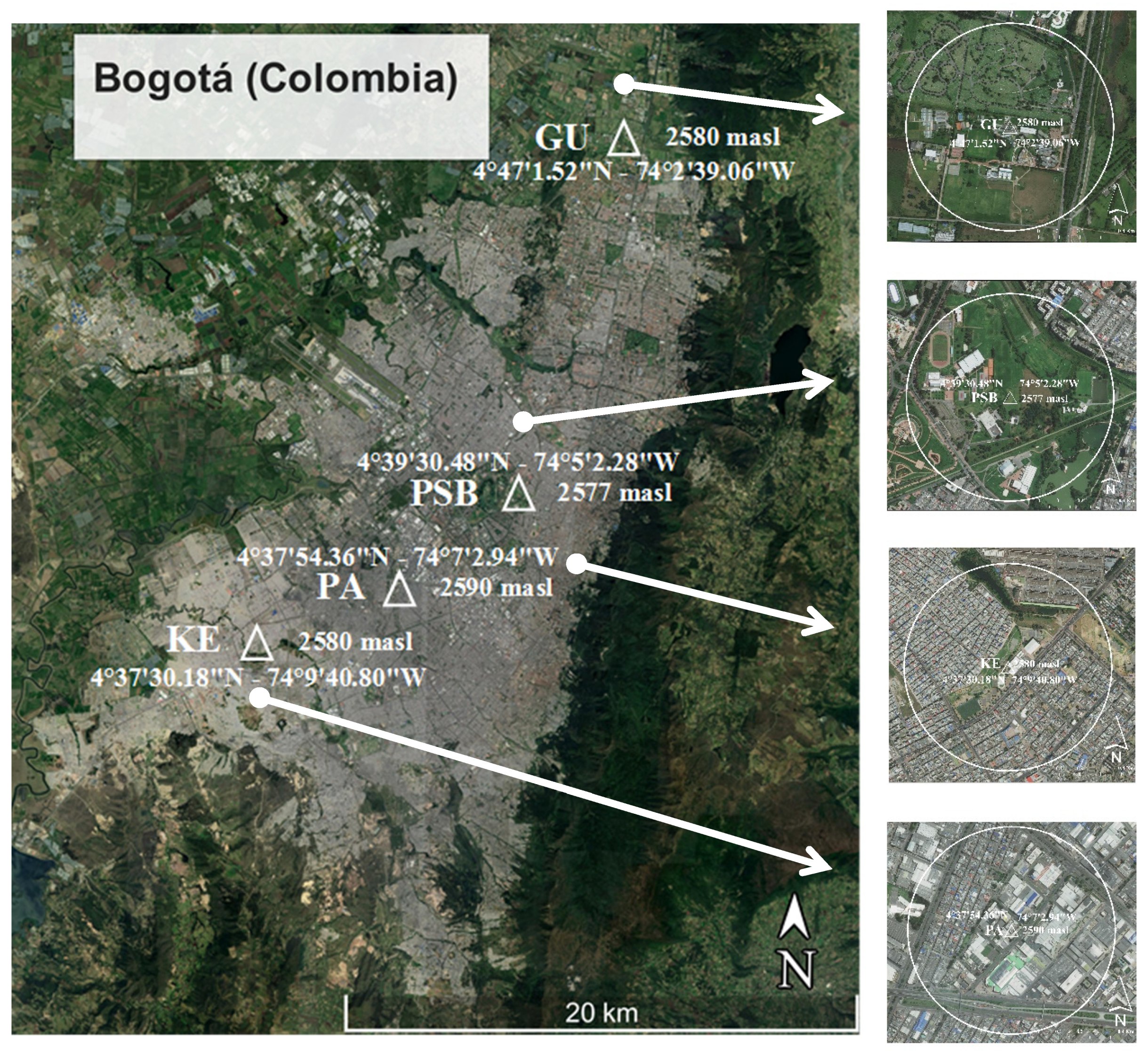
This study was conducted in the high-altitude tropical megacity of Bogotá, Colombia (4°35′57″ N; 74°04′51″ W). Four monitoring stations distributed throughout the megacity were established. The elevation of the monitoring stations was between 2577–2590 m.a.s.l. In this study, two monitoring stations were established where the predominant urban coverage was vegetated: Guaymaral = GU and Parque Simón Bolívar = PSB. In contrast, two monitoring stations were also established where the predominant urban coverage was impervious: Puente Aranda = PA and Kennedy = KE (Figure 1). On average, the annual climate characteristics of the study sites were as follows: Rainfall = 1091 mm, temperature = 12.9 °C, wind speed = 9.60 km/h, and relative humidity = 77.0%.
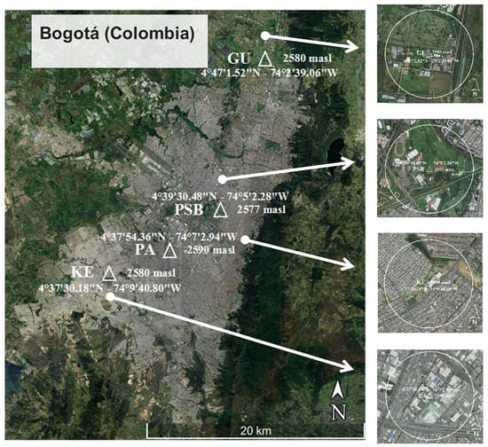
Figure 1.
Location of monitoring stations in the megacity of Bogotá, Colombia (Google Earth Pro, 2022).
2.2. Information Collection
Orthomosaics from 2010–2017 were used. These were downloaded from the Spatial Data Infrastructure Platform for the Capital District of Bogotá, Colombia [33]. Subsequently, maps were generated at each monitoring station on a scale of 1:5000. The maps were generated within a radius of 500 m in relation to the physical location of each monitoring station [34,35]. Within this radius of influence, the following types of urban coverage were identified: impervious coverage—IC (pavement, concrete, and buildings), vegetated coverage—VC (grass, uncovered soil, and trees), and water coverage—WC (rivers, lakes, and wetlands). The types of urban coverage were quantified using ArcGis software (Version 10.3, Esri, San Diego, CA, USA). In addition, climate information was collected at each monitoring station during the study period: 1 January 2010–31 December 2017. The climate information was downloaded from the Platform of the Air Quality Monitoring Network of Bogotá, Colombia [36]. The climate variables considered were the following: air temperature (Ta), wind speed (Va), and relative humidity (RH).
2.3. Information Analysis
Initially, a pre-processing of the climate information obtained at each monitoring station was conducted. The missing information in the time series of climate variables was completed using the normal ratio method [37]. Before completing the missing information, it was verified that the time series had more than 75% of the information from the study period considered. Subsequently, the existence of anomalies in the time series was analyzed using the double-mass method [38]. In relation to temperature, the months of greatest hourly variation during the same day were identified, taking as a reference their monthly average at the multi-year level. From the time series of climate variables, the mean radiant temperature (TMR) was calculated. This corresponded to the amount of radiation absorbed by the pedestrian during the day, where the sources were all the surfaces that surrounded him and the view factor that existed between the sources and the pedestrian [39]. The TMR considered both shortwave (direct, diffuse, and reflected) and longwave radiation (surrounding surfaces and from the atmosphere). The equations used for the calculation of TMR (°C) considered the guidelines of Sen and Nag [40]:
where, Td is the dew point temperature (°C), Ta is the air temperature (°C), RH is the relative humidity (%), Tg is the globe temperature (°C), Va is the wind speed (m/s), and TMR is the mean radiant temperature (°C).
From the calculated TMR, the OTC in each monitoring station was analyzed using the Physiological Equivalent Temperature (PET) index. This is due to its wide use to evaluate the effect of vegetated coverage on OTC (e.g., [34,41]). The PET index calculation was performed with RayMan Pro Beta software (Version 3.1, Meteorological Institute, University Freiburg, Baden-Württemberg, Germany) [42] and based on TMR. This software was selected for its wide use in OTC studies on low and non-seasonal latitudes, such as India [40] and Singapore [43]. The following simulation conditions proposed by Matzarakis and Amelung [44] were used: physiological profile of a man, 35 years old, 1.75 m in height, 75 kg in weight, with 0.90 of clothing (dressed without a coat), standing, and 80 W of metabolic activity (standing and resting). In addition, it was assumed that the influencing factors in anthropogenic heat were uniform at all monitoring stations. Namely, no variations in OTC associated with factors such as heating and cooling systems, traffic, and industries were considered. Validation of the calculated PET index using RayMan Pro Beta software (Version 3.1, Meteorological Institute, University Freiburg, Baden-Württemberg, Germany) was performed in two ways. Initially, the Universal Thermal Comfort Index (UTCI) calculated using RayMan Pro Beta software (Version 3.1, Meteorological Institute, University Freiburg, Baden-Württemberg, Germany) was compared with that calculated using the UTCI calculator [45]. Thus, differences in the calculation of the PET index were compared using these two free-use tools. Subsequently, linear correlation analyses were performed between the PET index calculated using RayMan Pro Beta software (Version 3.1, Meteorological Institute, University Freiburg, Baden-Württemberg, Germany) and the temperature values observed at the monitoring stations. A strong relationship between these two variables suggested adequate performance for the software used [40,42].
The current OTC was estimated for each study area during the 24 h and in the months detected with the greatest range of hourly temperature variation for the same day. The PET index was classified according to the following ranges [46]: <4 °C = Extreme cold stress, 4–8 °C = Strong cold stress, 8–13 °C = Moderate cold stress, 13–18 °C = Light cold stress, 18–23 °C = No thermal stress, and 23–29 °C = light heat stress. This was based on the PET range that was historically observed in the monitoring stations selected in the study megacity. Spatiotemporal analysis of the influence of vegetated coverage on the current OTC (PET index) was carried out based on the guidelines of Sun et al. [47]. The influence of the two types of predominant urban coverage (VC: vegetated coverage and IC: impervious coverage) on OTC was analyzed (Figure 1). This analysis was developed during the study period and at the following hours: 1:00, 7:00, 13:00, and 19:00 h.
The study of the influence of urban coverage under RCP scenarios was carried out for the month detected as the one with the greatest hourly variation in temperature for the same day, and with a simulation horizon to 2100. Future OTC was calculated from the Ta projection for the RCPs 4.5 and 8.5. In this analysis, the guidelines proposed by Aminipouri et al. [48] were followed and considering the increase in Ta predicted for the Bogotá city (Colombia). This temperature increase corresponded to 2.20 °C and 4.90 °C under the RCPs 4.5 and 8.5, respectively [30]. Thus, Va and RH were also projected under the previous RCPs in all monitoring stations and from their correlation with Ta (linear regression models). Then, TMR with Equations (1)–(3), and OTC through the PET index were estimated for these RCP scenarios. All these calculations were executed with RayMan Pro Beta software (Version 3.1, Meteorological Institute, University Freiburg, Baden-Württemberg, Germany). Lastly, forecasts were also made based on average values of minimum and maximum Ta observed during the study period.
Base on OTC calculated for scenarios RCP 4.5 and 8.5, influence of the ENSO phenomenon was simulated (ENSO scenario). For this purpose, average PET index during the study period (2010–2017) was determined and compared with the years in which the occurrence of the ENSO phenomenon was reported. Hourly differences observed in the PET index between these two time periods (average and occurrence of ENSO) were considered to analyze the influence of the ENSO phenomenon on OTC under the RCPs considered. During the study period, the occurrence of a strong ENSO was reported for 2010 (Oceanic Niño Index—ONI = 1.50 °C) [49]. This was the reference year to study the future influence of the ENSO phenomenon under the RCP scenarios considered. Therefore, in this study, three scenarios of information simulation and analysis were considered: (i) Current OTC, (ii) OTC under RCPs 4.5 and 8.5, and (iii) OTC under RCPs 4.5 and 8.5, and ENSO (El Niño). Lastly, the following statistical tests were applied for the analysis of the information: Kolmogov-Smirnov normality test (p-values > 0.050), Pearson correlation coefficient, t-Student test, and linear regression models. All statistical tests were applied using IBM-SPSS software (Version 19.0, IBM, New York, NY, USA) and with 95% confidence.
3. Results and Discussion
3.1. Urban Surface Coverage
The coverage analysis during the study period (2010–2017) allowed us to identify variations in each monitoring station (Table 1). For example, the results showed that in 2017 the monitoring stations with the highest vegetated coverage were GU (VC = 75.9%) and PSB (VC = 72.3%). In contrast, the PA and KE stations were those with the highest impervious coverage (IC: 83.1% and 75.8%) and the lowest vegetated coverage (VC: 16.9% and 24.2%), respectively. Only two monitoring stations showed water coverage (WC: GU = 4.40% and PSB = 3.90%), which was constant during the study period. In this study, there were two monitoring stations with a predominance of vegetated coverage and two stations with a predominance of impervious coverage to analyze the variation of urban OTC.

Table 1.
Spatial variation of urban surface coverage during the study period (2010–2017).
3.2. Current OTC
On average, the results showed during the study period that the months with the greatest range of hourly temperature variation for the same day were in order of importance January, February, and December. For example, at the GU station, the maximum hourly temperature variation in January, February, and December was 12.9 °C, 11.5 °C, and 11.3 °C, respectively. These months were prioritized to analyze the OTC of all the monitoring stations under study. The Institute of Hydrology, Meteorology, and Environmental Studies of Colombia also reported equivalent results [29]. They reported hourly temperature variations for the same day exceeding 10 °C at the GU and PSB stations. The analysis of OTC in the monitoring stations and for the most critical month (January) showed that the time interval of the highest thermal stress due to strong cold (PET: 4–8 °C) was between 1:00–7:00 h (Table 2). The OTC was improved as the day progressed. Thus, at 13:00 h, OTC was of stress due to light cold (PET: 13–18 °C). However, at night, a reduction in OTC was again observed. This was of moderate cold thermal stress (PET: 8–13 °C). The results suggested that during the month of greatest temperature variation (January) there was no time interval without outdoor thermal stress. This trend was also observed for the other months and throughout the study period in this high-altitude megacity (tropical mountain climate—cold). During the other months, there were fewer hourly variations in the PET index for the same day. Though, cold thermal stress remained.
Table 2.
Average values of PET index (°C) for January.
A comparative analysis was conducted between 2010, 2014, and 2017 in relation to the occurrence of the ENSO phenomenon and its influence on OTC. This is for the month with the greatest hourly variation of temperature on the same day (January). The results showed the occurrence of El Niño for 2010 (ONI = 1.50 °C, strong), La Niña for 2014 (ONI = −0.40 °C, weak), and La Niña for 2017 (ONI = −0.30 °C, weak) [49]. When analyzing the possible influence of the ENSO phenomenon, the results showed that during its occurrence in 2010, OTC tended to decrease during the most critical hour (7:00 h). On average, thermal stress due to strong cold increased between 25.2–38.6% (Table 2). However, OTC tended to increase slightly during the least critical hour (13:00 h). On average, light cold thermal stress decreased between 2.45–8.07% during this hour. In the study megacity, the ENSO phenomenon historically manifested itself as a period of dry weather (decrease in rainfall) and an increase in temperature [49]. Therefore, the results suggested for the high-altitude megacity under study (tropical mountain climate—cold) that the ENSO phenomenon tended to increase outdoor thermal stress more compared to outdoor thermal comfort. This is for the identified hours of lowest (7:00 h) and highest (13:00 h) OTC during the day, respectively. In the study sites, as the ENSO phenomenon is associated with a greater number of days of dry weather and increased temperature, it is likely that the above findings will be intensified in the future due to the global warming phenomenon. In other words, there will possibly be a greater hourly range of temperature variation and, therefore, greater outdoor thermal stress during the day.
Overall, OTC at study sites ranged from strong cold stress (PET: 4–8 °C) to moderate cold stress (PET: 13–18 °C) (Table 2). A t-Student test showed the existence of significant differences in the PET index between monitoring stations with different urban surface coverage: GU–PA (p-value = 0.005), GU–KE (p-value = 0.010), PSB–PA (p-value = 0.007), and PSB–KE (p-value = 0.210). As mentioned, the GU and PSB stations showed predominantly vegetated coverage (GU = 78.0% and PSB = 73.1%) compared to the PA and KE stations, where the predominant coverage was impervious (PA = 82.4% and KE = 76.9%). Therefore, the results suggested that OTC was influenced by the type of surface coverage predominant in the study stations. Obiakor et al. [50] reported similar results in urban areas. The radius of influence analyzed in our study was 500 m, in relation to the physical location of the selected monitoring stations.
On average, the results suggested comparatively that an increase between 55.0–60.5% in vegetated coverage generated an increase between 12.4–12.7% (PET: 1.28–1.31 °C) in urban OTC. This trend was more marked during the hours of greater OTC (13:00 h). In this case, OTC increased between 22.3–28.3% (2.87–3.53 °C). In contrast, this trend was less marked during the hours of lower OTC (7:00 h). At this time, OTC increased only between 1.49–12.4% (0.13–1.00 °C) (Figure 2). The results suggested for the high-altitude megacity under study that the increase in vegetated coverage tended to improve thermal comfort during the hours of lower thermal stress (13:00 h) compared to the hours of greater thermal stress (7:00 h). The difference observed in the improvement of OTC between these two hours was between 9.90–26.8% (1.87–3.40 °C). The previous results were consistent with those reported by Chow et al. [43] in Singapore, where at noon the highest values of OTC (PET) were observed in areas with a predominance of vegetated coverage, and the lowest values were observed in areas with a predominance of impervious coverage. In our study, the average ratio between the percentage increase in vegetated coverage and the percentage increase in OTC was 4.60. Namely, for every 10.0% increase in urban vegetation coverage, an increase of 0.22 °C in OTC was obtained.
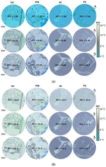
Figure 2.
Average PET index for (a) 7:00 h and (b) 13:00 h during January. PET: 4–8 °C = Stress/strong cold, 8–13 °C = Stress/moderate cold, 13–18 °C = Stress/light cold, and 18–23 °C = No thermal stress.
Additionally, the results showed, on average, that the hourly variation range of OTC in monitoring stations with a predominance of vegetated coverage was greater (PET range = 9.50 °C) compared to monitoring stations with a predominance of impervious coverage (PET range = 6.35 °C) (Figure 2). These findings indicated that monitoring stations with a predominance of impervious coverage tended to be more frequently in conditions of higher cold thermal stress (PET: 7.25–13.6 °C) compared to monitoring stations located in areas of predominance vegetated coverage (PET: 7.00–16.5 °C). During the study period, the outdoor thermal stress in the monitoring stations with a predominance of vegetated coverage (VC between 73.1–78.0%) was 1.29 °C lower compared to the monitoring stations with a predominance of impervious coverage (IC between 82.4–76.9%). Song and Wang [51] reported similar results in the City of Phoenix (USA).
As expected, there were no significant differences between the GU and PSB stations in relation to the PET index (p-value = 0.894). This is possibly due to the same type of urban surface coverage predominant in these two study stations: vegetated coverage (GU = 78.0% and PSB = 73.1%) (Figure 2). Likewise, between the PA and KE stations, there were no significant differences in relation to the PET index (p-value = 1.000). This trend was possibly associated with the predominant impervious coverage at these two monitoring stations (PA = 82.4% and KE = 76.9%). Therefore, consistency in the findings was observed from the analysis of the influence of urban surface coverage on OTC.
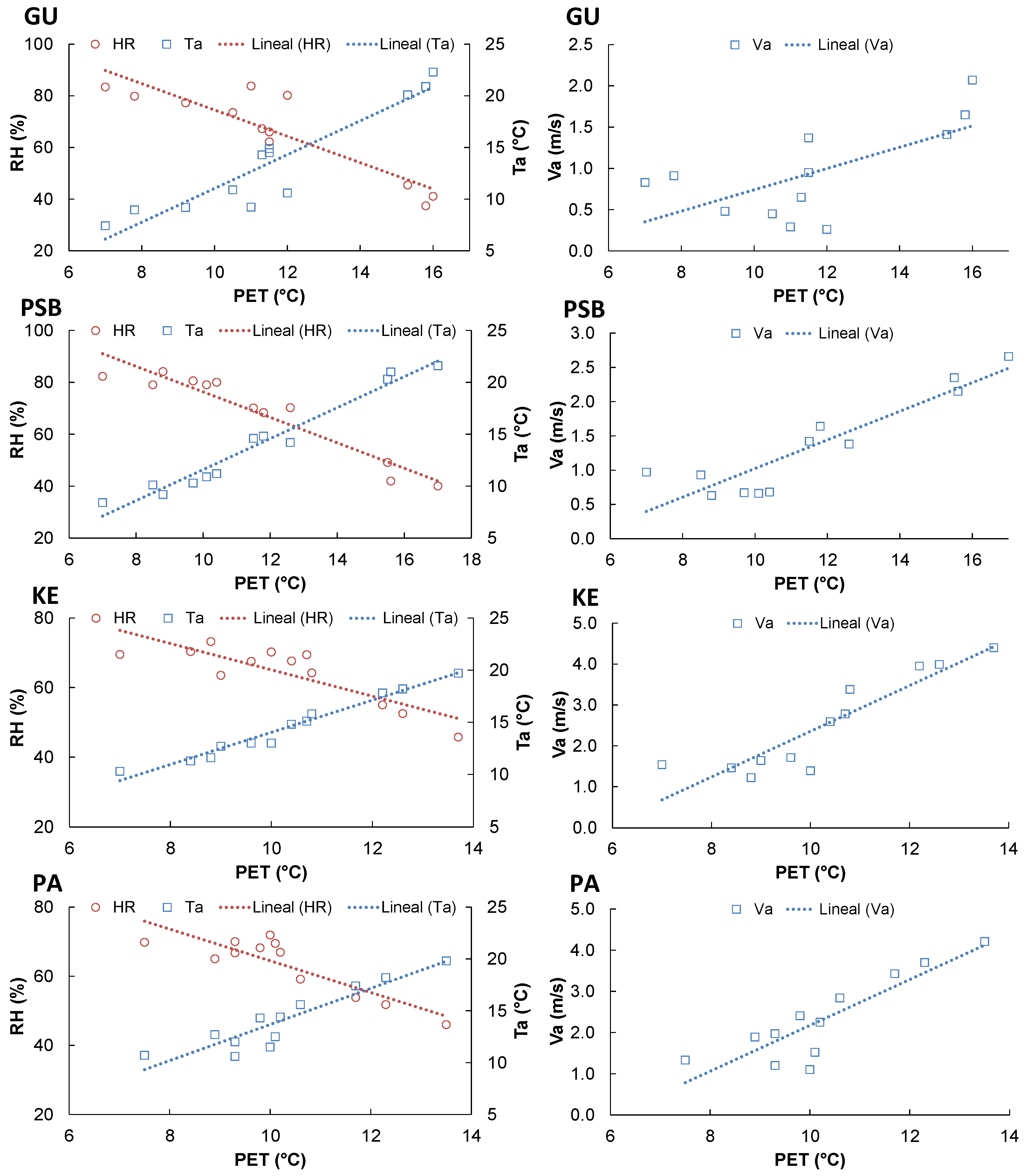
The results consistently showed that the climate variable that best correlated with the PET index at all monitoring stations was Ta. The relationship detected was direct and very strong (average r-Pearson = 0.955). This was the main climate variable that conditioned the PET index (Figure 3). However, the results showed differences for the other climate variables considered from the predominant urban surface coverage. In the monitoring stations with a predominance of vegetated coverage, the order of importance in the correlations between the PET index and the other climate variables was as follows: RH (average r-Pearson = −0.923) > Va (average r-Pearson = 0.784). Conversely, in stations with a predominance of impervious coverage the order of importance was as follows: Va (average r-Pearson = 0.890) > RH (average r-Pearson = −0.857). Therefore, the results suggested that in areas with a predominance of vegetated coverage (GU and PSB), RH had a greater influence on the PET index compared to Va. Conversely, in stations with a predominance of impervious coverage (KE and PA), Va had a greater influence compared to RH.
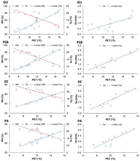
Figure 3.
Average trend of climate variables in relation to the PET index. Ta = Temperature, RH = Relative humidity, and Va = Wind speed.
Under the climate conditions of the study (tropical mountain climate—cold), the results showed that when Ta increased, the outdoor thermal stress due to cold decreased (PET) in all the monitoring stations considered (Figure 3). On average, in the monitoring stations with a predominance of vegetated coverage, for each increase of 1.0 °C in Ta, the OTC increased by 7.27% (0.84 °C). In the monitoring stations with a predominance of impervious coverage, for every increase of 1.0 °C in Ta, the OTC increased by 7.00% (0.72 °C). Comparatively, as Ta increased, OTC increased more rapidly in monitoring stations with vegetated coverage rather than in monitoring stations with impervious coverage. The findings also hinted that when RH decreased, OTC was increased in the high-altitude megacity under study. On average, in monitoring stations with a predominance of vegetated coverage, for every 10.0% decrease in RH, the OTC increased by 14.8% (1.71 °C). In monitoring stations with a predominance of impervious coverage, for every 10.0% decrease in RH, the OTC increased by 15.7% (1.61 °C).
The results showed that during the hours in which the highest wind speeds were observed, the greatest OTC was also observed. However, thinking in this study that when Va increased OTC also increased could be a mistake. These increases in Va towards the hour of greater OTC (13:00 h) were possibly related to atmospheric instability conditions in the high-altitude megacity under study [52]. If this trend had not occurred, OTC would have been greater during this time. When analyzing the trend of the main variables to determine OTC (Ta, RH, and Va), it was observed that, although there was a high Ta (18.0 °C) and a low RH (between 37.0–52%), an increase in Va (between 0.60 m/s–1.70 m/s) could reduce OTC, and therefore increase the outdoor thermal stress due to cold. A multiple linear regression analysis between the PET index (dependent variable) and the climate and coverage variables (independent variables) showed that there were no significant models for the study sites. In this study, the PET index could not be explained statistically from the type of urban coverage considered. This index could only be explained statistically from the three climate variables considered for its calculation (R2 ≥ 0.916, p-value < 0.001) (Figure 3).
Finally, during the validation of the selected software (RayMan Pro Beta software, Version 3.1, Meteorological Institute, University Freiburg, Ba-den-Württemberg, Germany)), a very strong linear correlation was evidenced between the calculated PET index and the temperature values observed in all monitoring stations (r-Pearson ≥ 0.920, p-value < 0.001). In addition, the results showed that the differences in the calculation of UTCI using the RayMan Pro Beta software (Version 3.1, Meteorological Institute, University Freiburg, Baden-Württemberg, Germany) and UTCI calculator [45] were between 0.26–2.62 °C. Therefore, in this study, the findings suggested good performance of the selected software.
3.3. RCP Scenarios
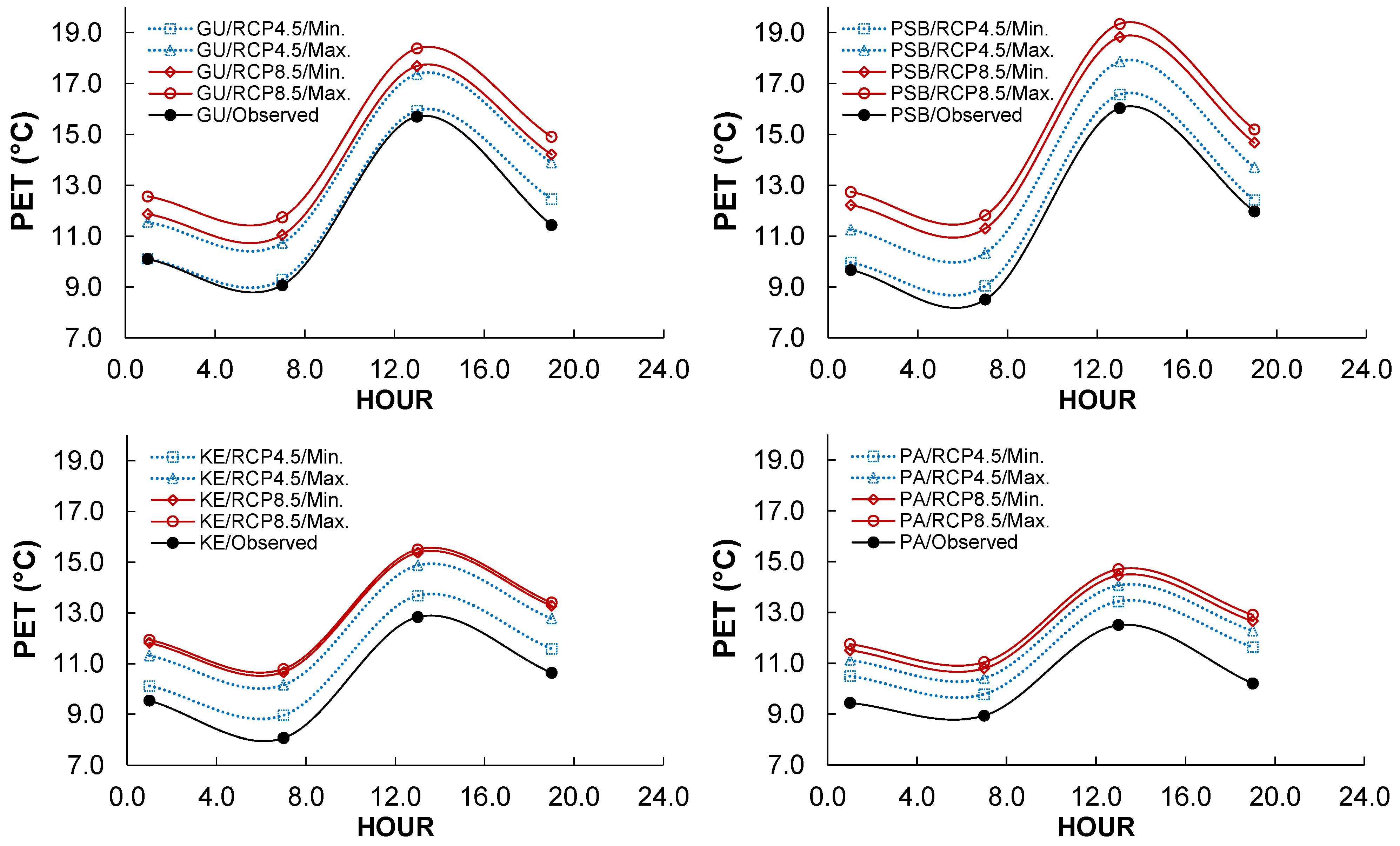
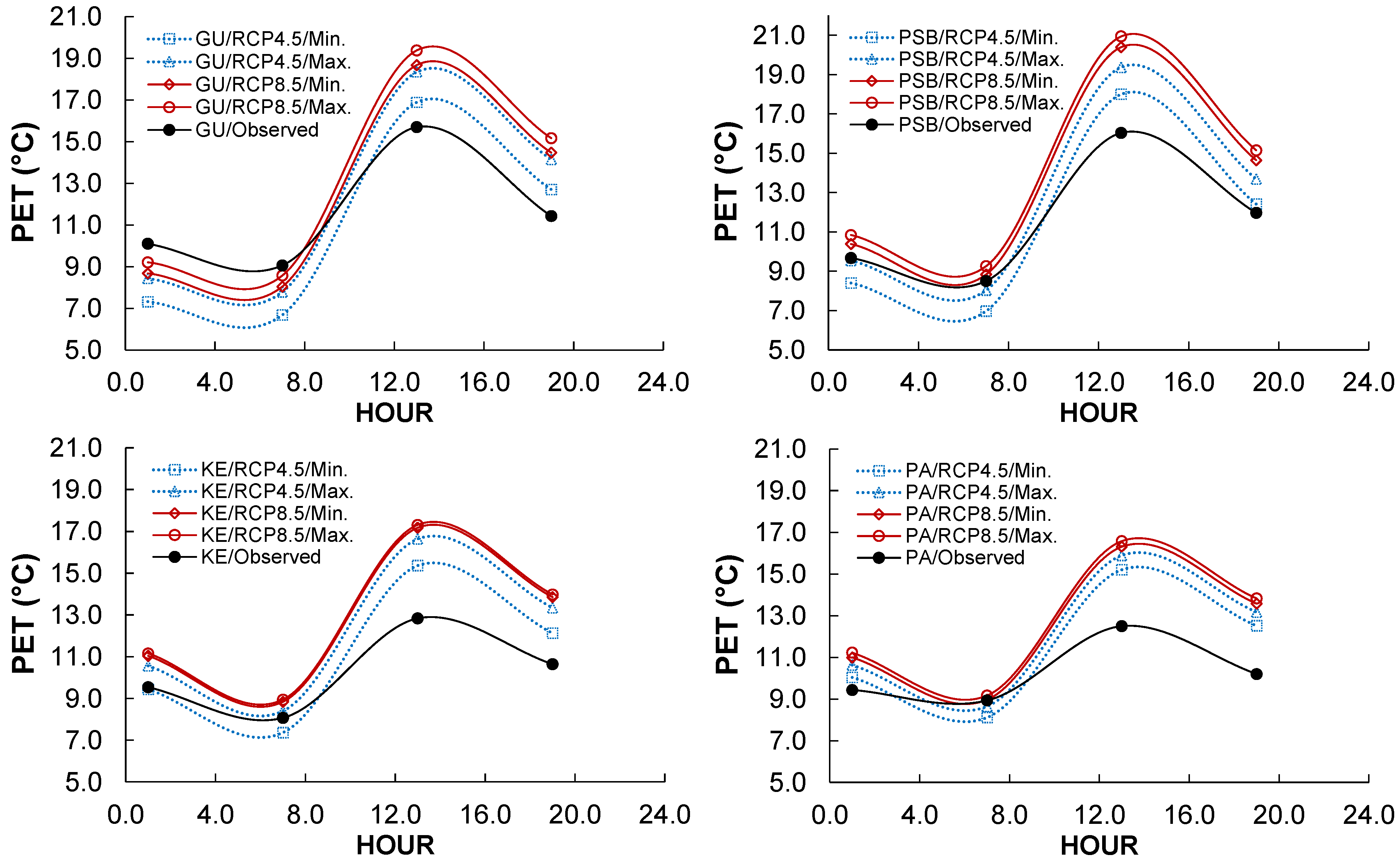
Overall, the results showed that OTC predicted under RCP scenarios (2070–2100) had a similar hourly trend compared to that observed during the baseline study period (2010–2017). This is based on the increases in the PET index forecast under the two RCP scenarios considered (RCPs 4.5 and 8.5). The results showed that the months with the greatest hourly temperature variation for the same day were in order of importance January, February, and December. Thus, OTC under RCP scenarios was evaluated for the most critical month (January). Figure 4 shows the observed average PET values, and the minimums and maximums forecast under the RCP scenarios considered for the most critical month.
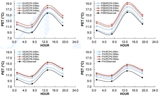
Figure 4.
Observed average PET values, and the minimums and maximums forecast under RCP scenarios at monitoring stations. PET: 4–8 °C = Stress/strong cold, 8–13 °C = Stress/moderate cold, 13–18 °C = Stress/light cold, and 18–23 °C = No thermal stress.
A t-Student test showed the existence of significant differences in the predicted PET index between monitoring stations with different urban surface coverage: GU–PA (p-values < 0.037), GU–KE (p-values < 0.004), PSB–PA (p-values < 0.027), and PSB–KE (p-values < 0.003). The results hinted at differences in predicted OTC from the type of coverage predominant in the study stations. As mentioned, vegetated coverage predominated at GU and PSB stations, and impervious coverage predominated at KE and PA stations. On average, greater differences were observed between monitoring stations with different coverage when considering the predicted maximum PET values (difference = 12.2%, 1.52 °C), compared to the predicted minimum PET values (difference = 9.12%, 1.09 °C). This is under each of the RCP scenarios considered (Figure 4). Therefore, the findings suggested that the differences in OTC between urban areas with a predominance of vegetated and impervious coverage were greater when maximum temperatures were observed under the RCP scenarios. The results also showed that the global warming phenomenon had a greater effect during the hour of lower OTC (7:00 h) compared to the hour of greater OTC (13:00 h). On average, regardless of the coverage type, the increase in PET at 7:00 h was 21.4% and at 13:00 h was 13.2%. The previous trend suggested that the global warming phenomenon had a lower impact during the hours of greater OTC (13:00 h) compared to the hours of lower OTC (7:00 h). This is under the particular high-altitude climate conditions of the tropical megacity under study.
On average, for the RCP4.5 scenario, the results suggested comparatively that an increase between 55.0–60.5% in vegetated coverage generated an increase between 8.36–13.5% (PET: 1.06–1.71 °C) in urban OTC. Namely, a decrease in moderate cold stress was observed. Under this scenario, during the hour of greatest OTC (13:00 h) it was observed that in the monitoring stations with a predominance of vegetated coverage the thermal stress was light cold. In monitoring stations with a predominance of impervious coverage, the outdoor thermal stress was similar (Figure 4). On average, for the RCP8.5 scenario, the findings comparatively hinted that an increase between 55.0–60.5% in vegetated coverage generated an increase between 8.57–14.0% (PET: 1.20–2.04 °C) in urban OTC. That is, cold stress decreased from moderate to light. During the hour of greatest OTC (13:00 h), it was observed that in the monitoring stations with a predominance of vegetated coverage the thermal stress was between light cold and without thermal stress. While in the monitoring stations with a predominance of impervious coverage there was always stress due to light cold. In the high-altitude tropical megacity under study, the results suggested that the effect of vegetated coverage on improving OTC increased as the phenomenon of global warming (RCP8.5) intensified. This compared to the urban coverage of impervious type. The global warming phenomenon under the scenarios RCPs 4.5 and 8.5 caused cold stress to decrease in the megacity under study.
Finally, under the RCP4.5 scenario, for each 10.0% increase in urban vegetation coverage, an average increase of 0.24 °C in OTC was obtained. Under the RCP8.5 scenario, for each 10.0% increase in urban vegetation coverage, an average increase of 0.28 °C in OTC was obtained. Without climate change scenarios, the average increase observed was 0.22 °C for each 10.0% increase in vegetated coverage. Therefore, the results suggested that the positive effect of vegetation on OTC increased as the global warming phenomenon intensified.
3.4. ENSO Scenario
In this study, the effect of climate change (RCPs 4.5 and 8.5) during the ENSO phenomenon (2070–2100) was considered. Under this scenario, the results showed that the months with the highest hourly temperature variation for the same day were in order of importance January, February, and December. Thus, OTC under the ENSO scenario was evaluated for that month of greatest variation in the PET index (January). Figure 5 shows the observed average PET values and those forecast under the ENSO scenario for January. A t-Student test showed the existence of significant differences in the predicted PET index between monitoring stations with different urban coverage: GU–PA (p-values < 0.019), GU–KE (p-values < 0.044), PSB–PA (p-values < 0.021), and PSB–KE (p-values < 0.040). As reported, vegetated coverage predominated at GU and PSB stations and impervious coverage predominated at KE and PA stations. On average, greater differences were observed between monitoring stations with different coverage when considering the predicted maximum PET values (difference = 12.2%, 0.53 °C), compared to the predicted minimum PET values (difference = 1.36%, 0.16 °C). This considers the ENSO scenario and each of the RCP scenarios. The results suggested that the difference in OTC between monitoring stations with different types of coverage (vegetated and impervious) was greater when maximum temperatures were observed under the ENSO scenario.
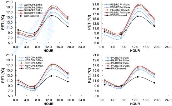
Figure 5.
Observed average PET values and the minimums and maximums forecast under the ENSO scenario at monitoring stations. PET: 4–8 °C = Stress/strong cold, 8–13 °C = Stress/moderate cold, 13–18 °C = Stress/light cold, and 18–23 °C = No thermal stress.
The results showed that under the ENSO scenario, OTC had a different behavior than that predicted for the RCP scenarios. In other words, cold stress increased during the hour of lower OTC (7:00 h) (Figure 5). This trend was most evident for monitoring stations with a predominance of vegetated coverage. On average, at the GU and PSB stations, OTC decreased by 16.6% (PET: 1.29 °C) and 2.74% (PET: 0.23 °C), respectively. In contrast, in the monitoring stations with a predominance of impervious coverage, no trend was appreciable during this hour. In the KE station, a slight increase was observed (3.89%, PET: 0.31 °C), and in the PA station, a slight decrease in OTC was observed (2.39%, PET: 0.21 °C). At this time, the outdoor thermal stress was between strong cold and moderate cold. During the hour of greatest OTC (13:00 h), in all monitoring stations, an increase in the PET index was observed regardless of the coverage type. However, this increase in OTC was stronger for monitoring stations with a predominance of impervious coverage. In the KE and PA stations (impervious coverage), the increase in OTC was 29.5% (PET: 3.79 °C) and 28.0% (PET: 3.50 °C), respectively. In the GU and PSB stations (vegetated coverage), the increase in OTC was 16.7% (PET: 2.62 °C) and 22.7% (PET: 3.64 °C), respectively. During this time, the outdoor thermal stress was between light cold and no thermal stress. Therefore, the results suggested that the ENSO phenomenon had a greater impact on the monitoring stations with a predominance of vegetated coverage during the hours of lower OTC (7:00 h). Conversely, the ENSO phenomenon had a greater impact on monitoring stations with a predominance of impervious coverage during the hours of greatest OTC (13:00 h).
On average, during the ENSO scenario, it was observed that the hourly variation range of OTC in monitoring stations with a predominance of vegetated coverage was greater (PET range = 11.0 °C) compared to monitoring stations with a predominance of impervious coverage (PET range = 7.80 °C) (Figure 5). The hourly ranges observed without ENSO and RCP scenarios were 1.16 and 1.23 times lower for vegetated and impermeable coverage stations, respectively (Figure 4). The results suggested that the hourly variation range of the PET index increased during the occurrence of the ENSO phenomenon. In other words, the ENSO phenomenon increased the range of outdoor thermal stress during the day in the high-altitude tropical megacity under study. Lastly, under the ENSO scenario, for each 10.0% increase in urban vegetated coverage, an average increase of 0.28 °C was obtained in OTC.
4. Conclusions
The results of this study on the influence of vegetation on the outdoor thermal comfort (PET) of a high-altitude tropical megacity (cold mountain climate) allow us to visualize the following conclusions:
- Hourly variation range of the current OTC in urban vegetated areas is greater (+3.15 °C) compared to impervious areas. Thus, the outdoor thermal stress due to cold in vegetated areas is 1.29 °C lower compared to impervious areas.
- The effect of vegetated coverage on the improvement of urban OTC increases as the phenomenon of global warming intensifies. On average, in the current, RCP4.5, and RCP8.5 scenarios, for each 10.0% increase in urban vegetation coverage, an increase of 0.22, 0.24, and 0.28 °C in OTC is obtained, respectively.
- ENSO scenario has a greater negative impact on vegetated areas during the hours of lower OTC (7:00 h). Conversely, the ENSO scenario has a greater positive impact on impervious areas during the hours of greater OTC (13:00 h).
- Hourly variation range of the PET index increases during the ENSO scenario: vegetated areas = +16.7% and impervious areas = +22.7%.
- On average, in the ENSO scenario, for each 10.0% increase in urban vegetated coverage, an increase of 0.28 °C in OTC is obtained. This trend is like that reported in the RCP8.5 scenario.
The following detected limitations should be considered to visualize future research lines: (i) the influence of anthropogenic heat (e.g., heating and cooling, transport, and industrial processes) was not considered in the simulations performed, and (ii) the analysis of coverage was simplified, i.e., only urban areas with a predominance of vegetated or impervious coverages were considered. Indeed, a more detailed study on OTC requires consideration of all types of coverage existing in a megacity. Lastly, in the context of climate change and variability, this study constitutes a reference point for decision-makers in public and private organizations to evaluate possible planning options for improving OTC in megacities.
Author Contributions
Conceptualization, A.M.B.-Z. and C.A.Z.-M.; methodology, A.M.B.-Z., C.A.Z.-M. and H.A.R.-Q.; validation and formal analysis, A.M.B.-Z., C.A.Z.-M. and H.A.R.-Q.; resources, A.M.B.-Z., C.A.Z.-M. and H.A.R.-Q.; writing—original draft preparation, A.M.B.-Z. and C.A.Z.-M.; writing—review and editing, A.M.B.-Z., C.A.Z.-M. and H.A.R.-Q.; funding acquisition, A.M.B.-Z., C.A.Z.-M. and H.A.R.-Q. All authors have read and agreed to the published version of the manuscript.
Funding
This research received no external funding.
Institutional Review Board Statement
Not applicable.
Informed Consent Statement
Not applicable.
Data Availability Statement
Not applicable.
Acknowledgments
The authors appreciate the academic support of the Universidad Distrital Francisco José de Caldas (Colombia) and of the INDESOS and GIIAUD research groups.
Conflicts of Interest
The authors declare no conflict of interest.
References
- Brown, S.; Nicholls, R.; Lázár, A.N.; Hornby, D.; Hill, C.; Hazra, S.; Addo, K.A.; Haque, A.; Caesar, J.; Tompkins, E.L. What are the implications of sea-level rise for a 1.5, 2 and 3 °C rise in global mean temperatures in the Ganges-Brahmaputra-Meghna and other vulnerable deltas? Reg. Environ. Chang. 2018, 18, 1829–1842. [Google Scholar] [CrossRef] [Green Version]
- Matthews, T. Humid heat and climate change. Prog. Phys. Geogr. Earth Environ. 2018, 42, 391–405. [Google Scholar] [CrossRef] [Green Version]
- McMichael, A.J.; Woodruff, R.E.; Hales, S. Climate change and human health: Present and future risks. Lancet 2006, 367, 859–869. [Google Scholar] [CrossRef]
- Najafzadeh, F.; Mohammadzadeh, A.; Ghorbanian, A.; Jamali, S. Spatial and Temporal Analysis of Surface Urban Heat Island and Thermal Comfort Using Landsat Satellite Images between 1989 and 2019: A Case Study in Tehran. Remote Sens. 2021, 13, 4469. [Google Scholar] [CrossRef]
- Pigliautile, I.; Pisello, A.; Bou-Zeid, E. Humans in the city: Representing outdoor thermal comfort in urban canopy models. Renew. Sustain. Energy Rev. 2020, 133, 110103. [Google Scholar] [CrossRef]
- Silva, J.S.; da Silva, R.M.; Santos, C.A.G. Spatiotemporal impact of land use/land cover changes on urban heat islands: A case study of Paço do Lumiar, Brazil. Build. Environ. 2018, 136, 279–292. [Google Scholar] [CrossRef]
- Solano–Olivares, K.; Romero, R.; Santoyo, E.; Herrera, I.; Galindo–Luna, Y.; Rodríguez–Martínez, A.; Santoyo-Castelazo, E.; Cerezo, J. Life cycle assessment of a solar absorption air-conditioning system. J. Clean. Prod. 2019, 240, 118206. [Google Scholar] [CrossRef]
- Crutzen, P.J.; Mosier, A.R.; Smith, K.A.; Winiwarter, W. N2O Release from Agro-biofuel Production Negates Global Warming Reduction by Replacing Fossil Fuels. In A Pioneer on Atmospheric Chemistry and Climate Change in the Anthropocene; Crutzen, P.J., Brauch, H.G., Eds.; Springer International Publishing: Cham, Switzerland, 2016; pp. 227–238. [Google Scholar] [CrossRef] [Green Version]
- Tan, M.L.; Juneng, L.; Tangang, F.T.; Chung, J.X.; Firdaus, R.B.R. Changes in temperature extremes and their relationship with ENSO in Malaysia from 1985 to 2018. Int. J. Clim. 2021, 41, E2564–E2580. [Google Scholar] [CrossRef]
- Taleghani, M. Outdoor thermal comfort by different heat mitigation strategies–A review. Renew. Sustain. Energy Rev. 2018, 81, 2011–2018. [Google Scholar] [CrossRef]
- IPCC. Climate Change 2013—The Physical Science Basis: Working Group I; Contribution to the Fifth Assessment Report of the Intergovernmental Panel on Climate Change; Intergovernmental Panel on Climate Change, Ed.; Cambridge University Press: Cambridge, UK, 2014. [Google Scholar] [CrossRef] [Green Version]
- Bienvenido-Huertas, D.; Rubio-Bellido, C.; Marín-García, D.; Canivell, J. Influence of the Representative Concentration Pathways (RCP) scenarios on the bioclimatic design strategies of the built environment. Sustain. Cities Soc. 2021, 72, 103042. [Google Scholar] [CrossRef]
- Nilawar, A.P.; Waikar, M.L. Impacts of climate change on streamflow and sediment concentration under RCP 4.5 and 8.5: A case study in Purna river basin, India. Sci. Total Environ. 2019, 650, 2685–2696. [Google Scholar] [CrossRef]
- Kim, H.G.; Lee, D.K.; Park, C.; Kil, S.; Son, Y.; Park, J.H. Evaluating landslide hazards using RCP 4.5 and 8.5 scenarios. Environ. Earth Sci. 2015, 73, 1385–1400. [Google Scholar] [CrossRef]
- Zhou, P.; Liu, Z.; Cheng, L. An alternative approach for quantitatively estimating climate variability over China under the effects of ENSO events. Atmos. Res. 2020, 238, 104897. [Google Scholar] [CrossRef]
- Diniz, F.R.; Iwabe, C.M.N.; Piacenti-Silva, M. Valuation of the human thermal discomfort index for the five Brazilian regions in the period of El Niño-Southern Oscillation (ENSO). Int. J. Biometeorol. 2019, 63, 1507–1516. [Google Scholar] [CrossRef] [PubMed]
- Ren, H.-L.; Zheng, F.; Luo, J.-J.; Wang, R.; Liu, M.; Zhang, W.; Zhou, T.; Zhou, G. A Review of Research on Tropical Air-Sea Interaction, ENSO Dynamics, and ENSO Prediction in China. J. Meteorol. Res. 2019, 34, 43–62. [Google Scholar] [CrossRef]
- McGregor, G.R.; Ebi, K. El Niño Southern Oscillation (ENSO) and Health: An Overview for Climate and Health Researchers. Atmosphere 2018, 9, 282. [Google Scholar] [CrossRef] [Green Version]
- Johansson, E.; Thorsson, S.; Emmanuel, R.; Krüger, E. Instruments and methods in outdoor thermal comfort studies–The need for standardization. In Proceedings of the Urban Climate, ICUC8: The 8th International Conference on Urban Climate and the 10th Symposium on the Urban Environment, Dublin, Ireland, 1 January 2014; Volume 10, pp. 346–366. [Google Scholar] [CrossRef] [Green Version]
- Shooshtarian, S.; Lam, C.K.C.; Kenawy, I. Outdoor thermal comfort assessment: A review on thermal comfort research in Australia. Build. Environ. 2020, 177, 106917. [Google Scholar] [CrossRef]
- Tahbaz, M. Psychrometric chart as a basis for outdoor thermal analysis. Iran Univ. Sci. Technol. 2011, 21, 95–109. [Google Scholar]
- Tung, C.-H.; Chen, C.-P.; Tsai, K.-T.; Kántor, N.; Hwang, R.-L.; Matzarakis, A.; Lin, T.-P. Outdoor thermal comfort characteristics in the hot and humid region from a gender perspective. Int. J. Biometeorol. 2014, 58, 1927–1939. [Google Scholar] [CrossRef] [PubMed]
- Haldi, F.; Robinson, D. Modelling occupants’ personal characteristics for thermal comfort prediction. Int. J. Biometeorol. 2011, 55, 681–694. [Google Scholar] [CrossRef] [PubMed]
- Patiño, E.D.L.; Vakalis, D.; Touchie, M.; Tzekova, E.; Siegel, J. Thermal comfort in multi-unit social housing buildings. Build. Environ. 2018, 144, 230–237. [Google Scholar] [CrossRef]
- Golasi, I.; Salata, F.; Vollaro, E.D.L.; Coppi, M.; Vollaro, A.D.L. Thermal Perception in the Mediterranean Area: Comparing the Mediterranean Outdoor Comfort Index (MOCI) to Other Outdoor Thermal Comfort Indices. Energies 2016, 9, 550. [Google Scholar] [CrossRef] [Green Version]
- Zain, Z.M.; Taib, M.N.; Baki, S.M.S. Hot and humid climate: Prospect for thermal comfort in residential building. In Proceedings of the Ninth Arab International Conference on Solar Energy (AICSE-9), Manama, Bahrain, 30 April 2007; Volume 209, pp. 261–268. [Google Scholar] [CrossRef]
- Aljawabra, F.; Nikolopoulou, M. Influence of hot arid climate on the use of outdoor urban spaces and thermal com-fort: Do cultural and social backgrounds matter? Intell. Build. Int. 2010, 2, 198–217. [Google Scholar] [CrossRef]
- Lai, D.; Liu, W.; Gan, T.; Liu, K.; Chen, Q. A review of mitigating strategies to improve the thermal environment and thermal comfort in urban outdoor spaces. Sci. Total Environ. 2019, 661, 337–353. [Google Scholar] [CrossRef]
- IDEAM. La Variabilidad Climática y el Cambio Climático en Colombia; Instituto de Hidrología, Me-Teorología y Estudios Ambientales: Bogotá, Colombia, 2018. [Google Scholar]
- IDEAM. Modelo Institucional del IDEAM Sobre el Efecto Climático de los Fenómenos El Niño y La Niña en Colombia (No. 063–2007); Instituto de Hidrología, Meteorología y Estudios Ambientales: Bogotá, Colombia, 2007. [Google Scholar]
- Ramírez-Aguilar, E.A.; Souza, L.C.L. Urban form and population density: Influences on Urban Heat Island intensities in Bogotá, Colombia. Urban Clim. 2019, 29, 100497. [Google Scholar] [CrossRef]
- Anselm, N.; Rojas, O.; Brokamp, G.; Schütt, B. Spatiotemporal Variability of Precipitation and Its Statistical Relations to ENSO in the High Andean Rio Bogotá Watershed, Colombia. Earth Interact. 2020, 24, 1–17. [Google Scholar] [CrossRef]
- Ideca: Infraestructura de Datos Espaciales para el Distrito Capital. Available online: https://www.ideca.gov.co/ (accessed on 15 January 2018).
- Meili, N.; Acero, J.A.; Peleg, N.; Manoli, G.; Burlando, P.; Fatichi, S. Vegetation cover and plant-trait effects on outdoor thermal comfort in a tropical city. Build. Environ. 2021, 195, 107733. [Google Scholar] [CrossRef]
- Zafra, C.; Ángel, Y.; Torres, E. ARIMA analysis of the effect of land surface coverage on PM 10 concentrations in a high-altitude megacity. Atmospheric Pollut. Res. 2017, 8, 660–668. [Google Scholar] [CrossRef]
- RMCAB: Red de Monitoreo de Calidad del Aire de Bogotá. Available online: http://201.245.192.252:81/Report/stationreport (accessed on 15 January 2018).
- Tang, W.; Kassim, A.; Abubakar, S. Comparative studies of various missing data treatment methods–Malaysian experience. Atmos. Res. 1996, 42, 247–262. [Google Scholar] [CrossRef]
- Li, D.; Lu, X.X.; Yang, X.; Chen, L.; Lin, L. Sediment load responses to climate variation and cascade reservoirs in the Yangtze River: A case study of the Jinsha River. Geomorphology 2018, 322, 41–52. [Google Scholar] [CrossRef]
- Krüger, E.L.; Minella, F.O.; Matzarakis, A. Comparison of different methods of estimating the mean radiant temperature in outdoor thermal comfort studies. Int. J. Biometeorol. 2014, 58, 1727–1737. [Google Scholar] [CrossRef]
- Sen, J.; Nag, P.K. Effectiveness of human-thermal indices: Spatio–temporal trend of human warmth in tropical India. Urban Clim. 2019, 27, 351–371. [Google Scholar] [CrossRef]
- Farhadi, H.; Faizi, M.; Sanaieian, H. Mitigating the urban heat island in a residential area in Tehran: Investigating the role of vegetation, materials, and orientation of buildings. Sustain. Cities Soc. 2019, 46, 101448. [Google Scholar] [CrossRef]
- Matzarakis, A.; Rutz, F.; Mayer, H. Modelling radiation fluxes in simple and complex environments: Basics of the RayMan model. Int. J. Biometeorol. 2010, 54, 131–139. [Google Scholar] [CrossRef] [Green Version]
- Chow, W.T.; Akbar, S.N.B.A.; Heng, S.L.; Roth, M. Assessment of measured and perceived microclimates within a tropical urban forest. Urban For. Urban Green. 2016, 16, 62–75. [Google Scholar] [CrossRef] [Green Version]
- Matzarakis, A.; Amelung, B. Physiological Equivalent Temperature as Indicator for Impacts of Climate Change on Thermal Comfort of Humans. In Seasonal Forecasts, Climatic Change and Human Health; Health and Climate, Advances in Global Change Research; Thomson, M.C., Garcia-Herrera, R., Beniston, M., Eds.; Springer: Dordrecht, The Netherlands, 2008; pp. 161–172. [Google Scholar] [CrossRef]
- IfADo: Leibniz Research Centre for Working Environment and Human Factors. Available online: http://www.utci.org/utcineu/utcineu.php (accessed on 15 February 2019).
- Zare, S.; Hasheminejad, N.; ElahiShirvan, H.; Hemmatjo, R.; Sarebanzadeh, K.; Ahmadi, S.; Zare, S.; Hasheminejad, N.; ElahiShirvan, H.; Hemmatjo, R.; et al. Comparing Universal Thermal Climate Index (UTCI) with selected thermal indices/environmental parameters during 12 months of the year. Weather Clim. Extrem. 2018, 19, 49–57. [Google Scholar] [CrossRef]
- Sun, S.; Xu, X.; Lao, Z.; Liu, W.; Li, Z.; Garcia, E.H.; He, L.; Zhu, J. Evaluating the impact of urban green space and landscape design parameters on thermal comfort in hot summer by numerical simulation. Build. Environ. 2017, 123, 277–288. [Google Scholar] [CrossRef]
- Aminipouri, M.; Rayner, D.; Lindberg, F.; Thorsson, S.; Knudby, A.J.; Zickfeld, K.; Middel, A.; Krayenhoff, E.S. Urban tree planting to maintain outdoor thermal comfort under climate change: The case of Vancouver’s local climate zones. Build. Environ. 2019, 158, 226–236. [Google Scholar] [CrossRef]
- NOAA. NOAA’s Climate Prediction Center. Available online: https://origin.cpc.ncep.noaa.gov/products/analysis_monitoring/ensostuff/ONI_v5.php (accessed on 22 March 2022).
- Obiakor, M.O.; Ezeonyejiaku, C.D.; Mogbo, T.C. Effects of Vegetated and Synthetic (Impervious) Surfaces on the Microclimate of Urban Area. J. Appl. Sci. Environ. Manag. 2012, 16, 85–94. [Google Scholar] [CrossRef]
- Song, J.; Wang, Z.-H. Impacts of mesic and xeric urban vegetation on outdoor thermal comfort and microclimate in Phoenix, AZ. Build. Environ. 2015, 94, 558–568. [Google Scholar] [CrossRef] [Green Version]
- Zafra, C.; Suárez, J.; Pachón, J. Public Health Considerations for PM10 in a High-Pollution Megacity: Influences of Atmospheric Condition and Land Coverage. Atmosphere 2021, 12, 118. [Google Scholar] [CrossRef]

Publisher’s Note: MDPI stays neutral with regard to jurisdictional claims in published maps and institutional affiliations. |
© 2022 by the authors. Licensee MDPI, Basel, Switzerland. This article is an open access article distributed under the terms and conditions of the Creative Commons Attribution (CC BY) license (https://creativecommons.org/licenses/by/4.0/).