
Three-Dimensional Morphology and Watershed-Algorithm-Based Method for Pitting Corrosion Evaluation


Abstract
1. Introduction
2. Experiment Procedure
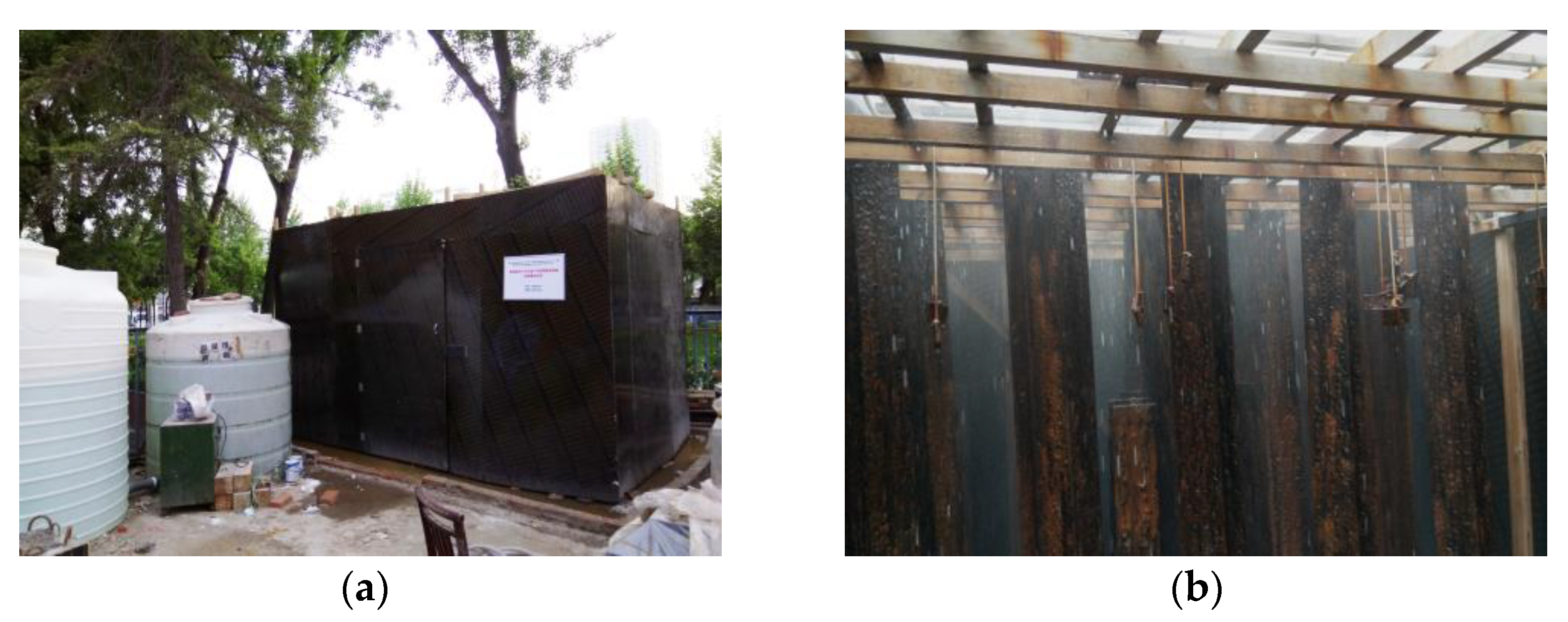
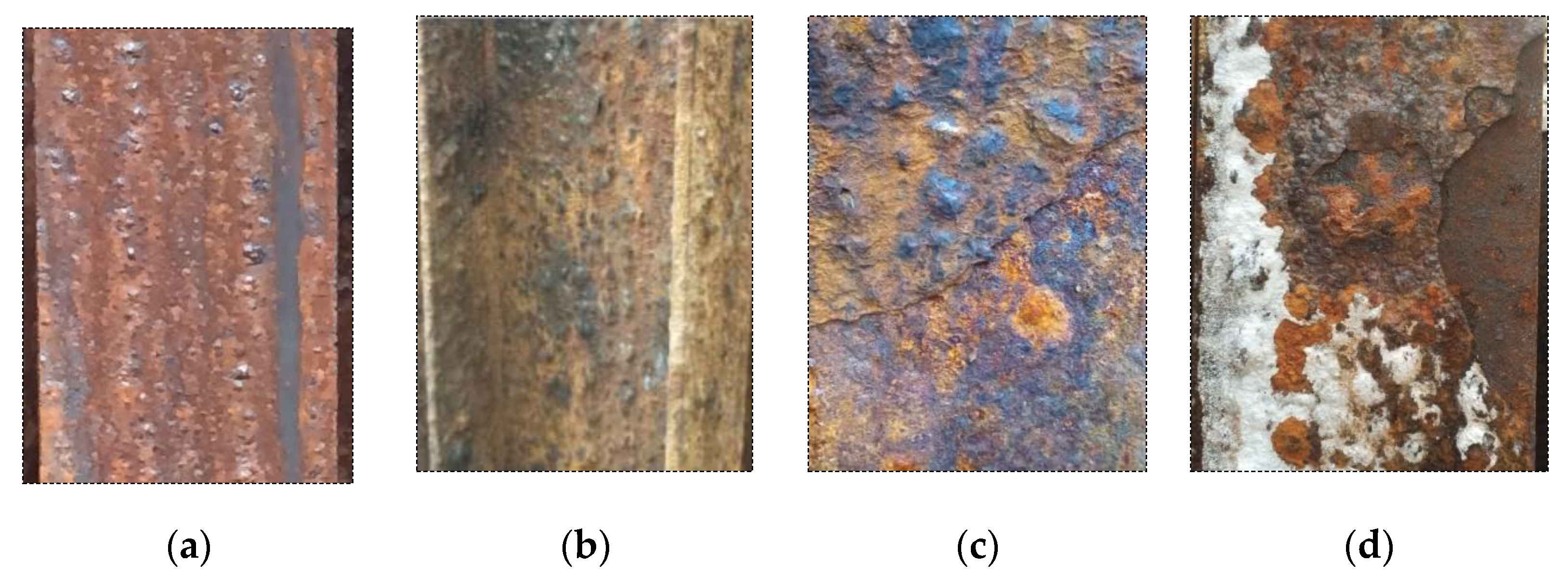
2.1. Accelerated Corrosion Test of H-Beams
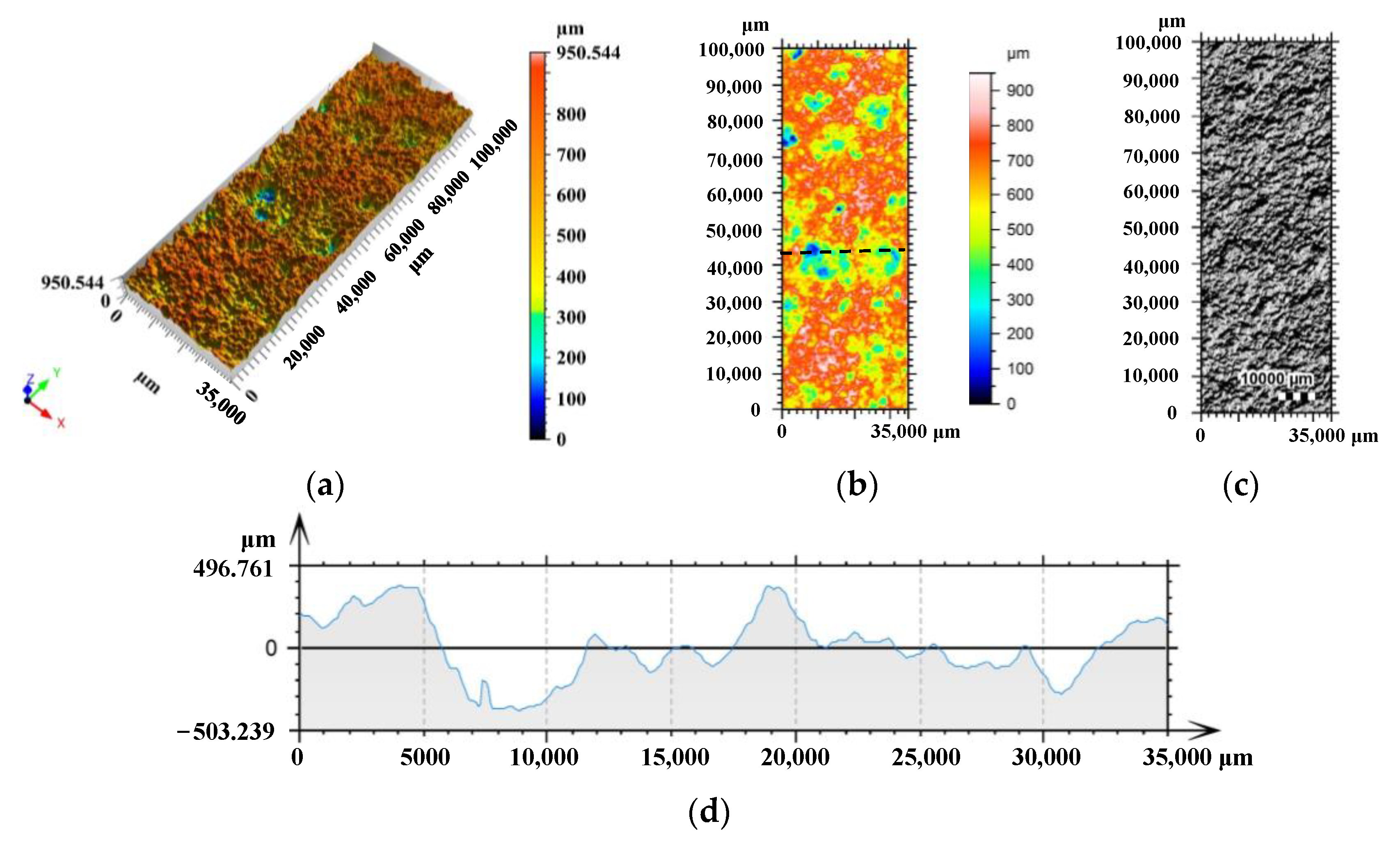
2.2. Three-Dimensional Morphological Scanning of Corroded Steel Plates
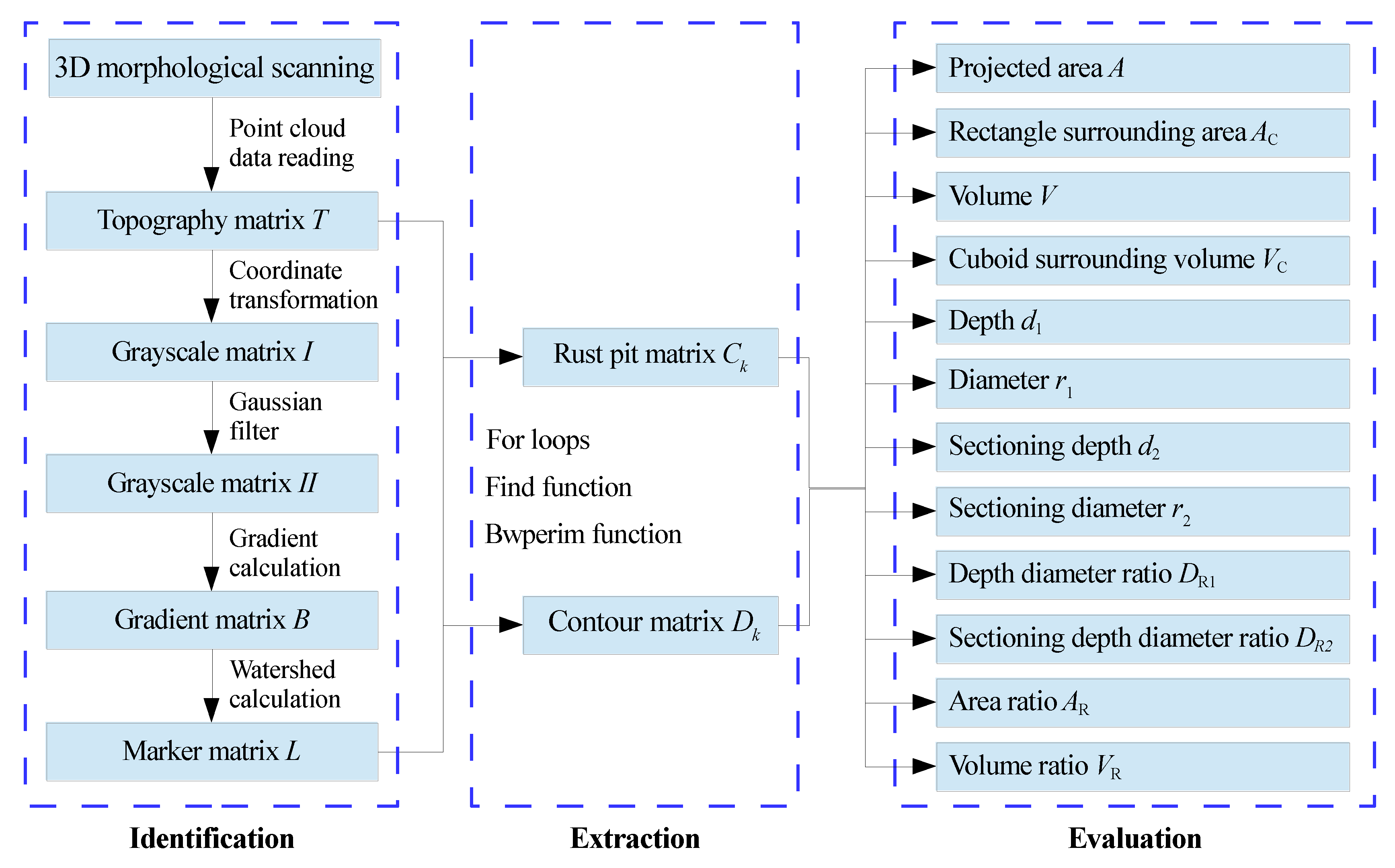
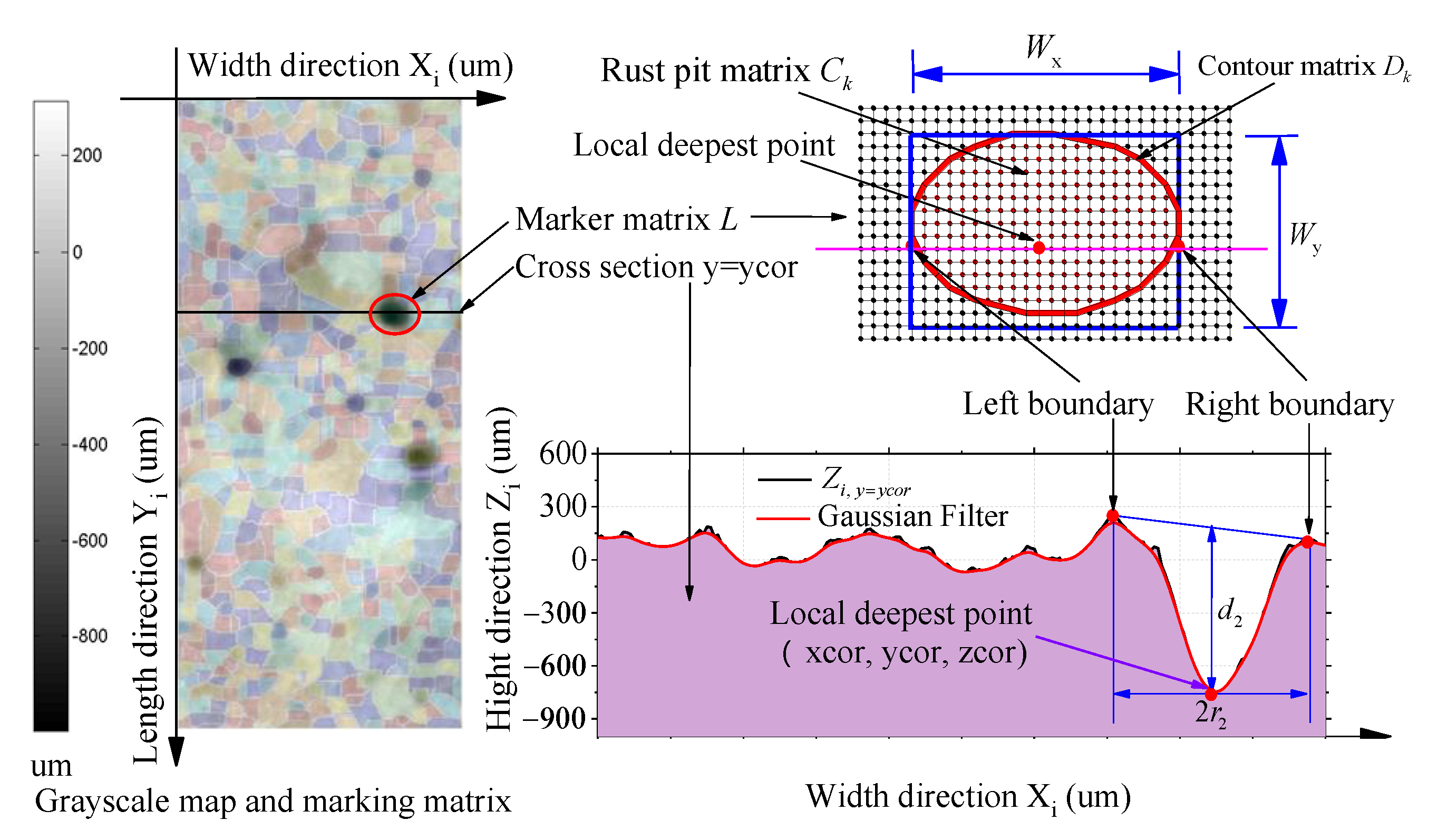
3. Identification, Extraction, and Evaluation Method for Rust Pits
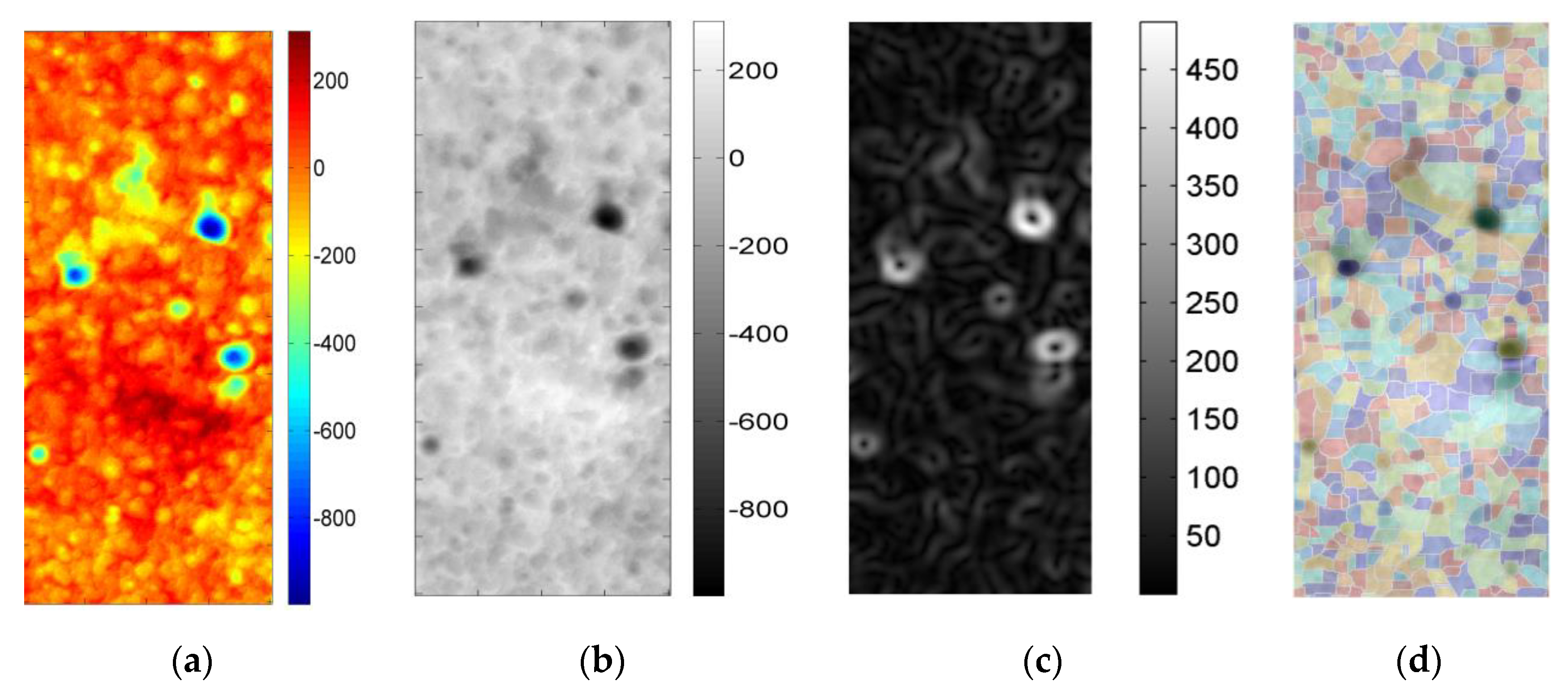
3.1. Method of Identifying and Extracting Surface Rust Pits
3.2. Method of Calculating the Size and Shape of Rust Pits
4. Results and Discussion
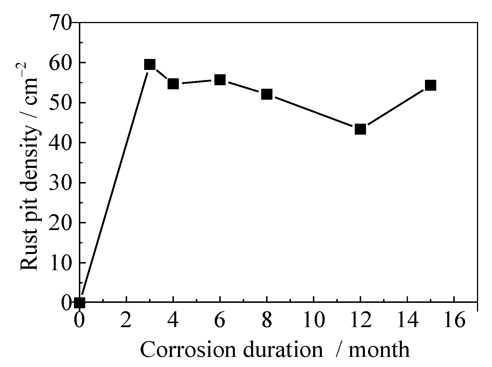
4.1. Rust Pit Density
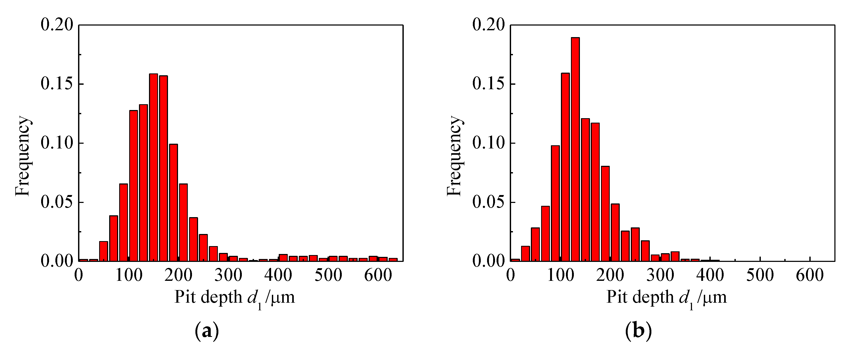
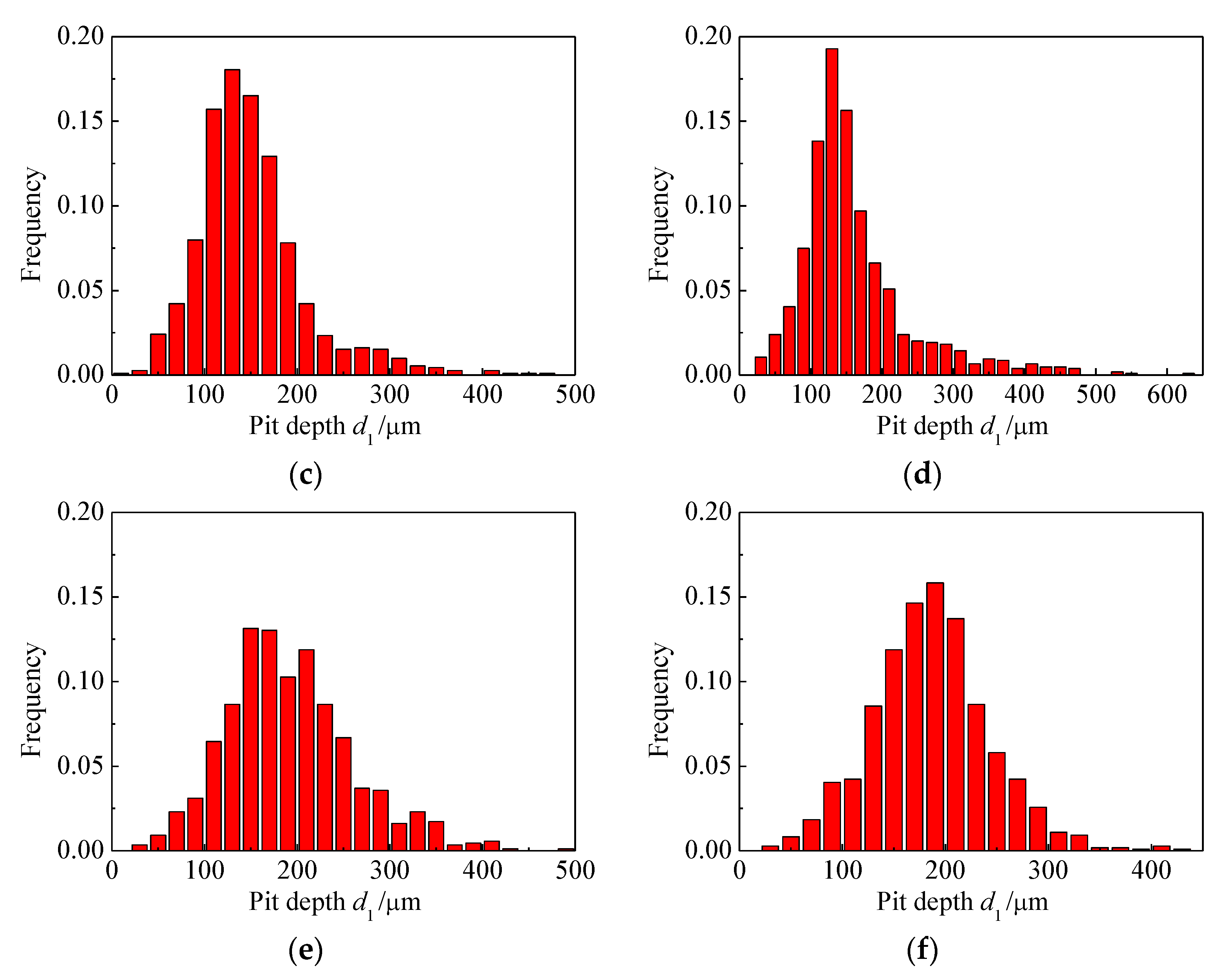
4.2. Rust Pit Size
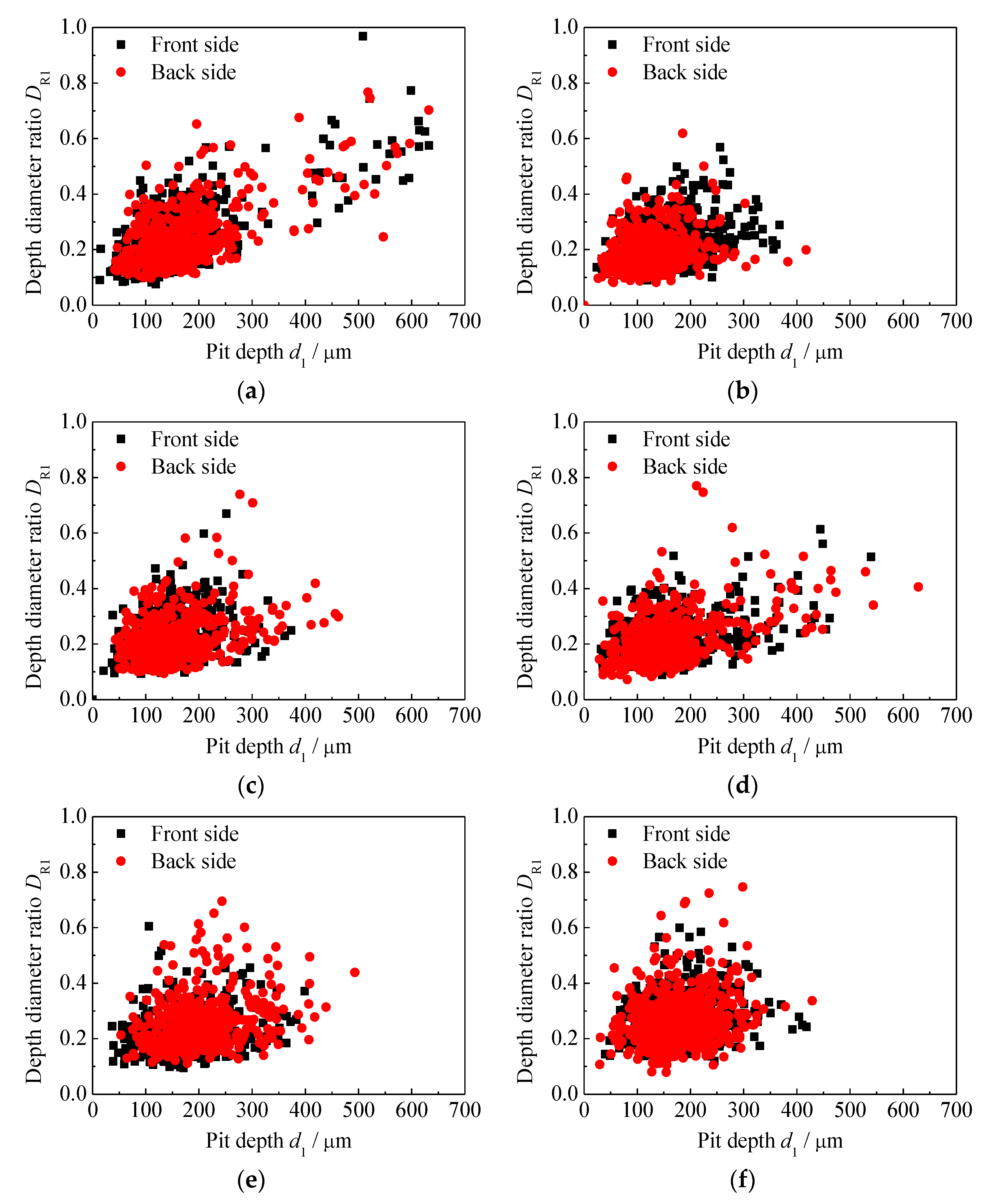
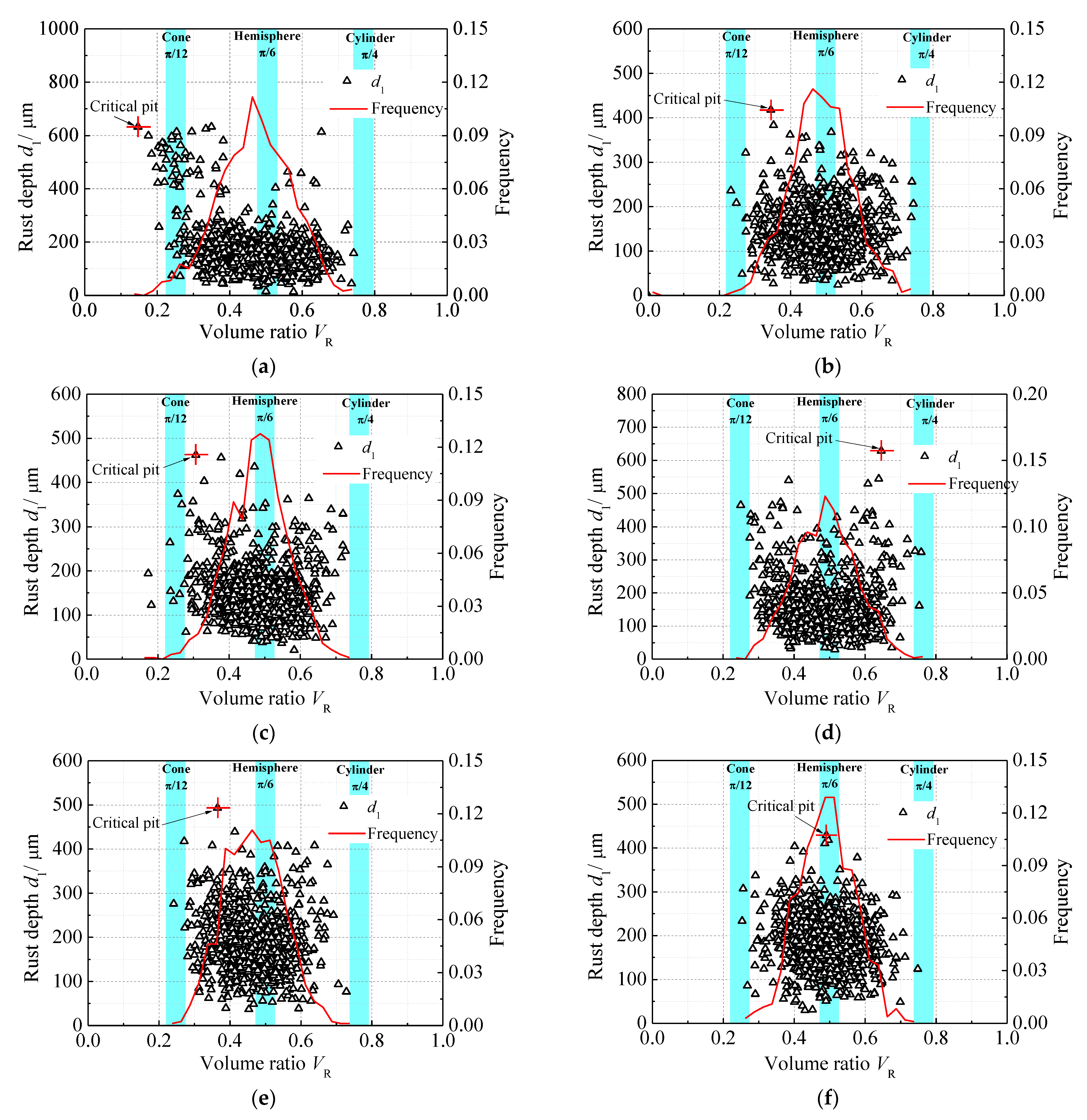
4.3. Rust Pit Shape
5. Conclusions
Author Contributions
Funding
Data Availability Statement
Conflicts of Interest
References
- Xu, S.; Wang, H.; Li, A.; Wang, Y.; Su, L. Effects of corrosion on surface characterization and mechanical properties of butt-welded joints. J. Constr. Steel Res. 2016, 126, 50–62. [Google Scholar] [CrossRef]
- Wang, Y.; Zhou, X.; Wang, H.; Kong, D.; Xu, S. Stochastic constitutive model of structural steel based on random field of corrosion depth. Case Stud. Constr. Mater. 2022, 16, e00972. [Google Scholar] [CrossRef]
- Li, A.; Xu, S.; Wang, Y.; Wu, C.; Nie, B. Fatigue behavior of corroded steel plates strengthened with CFRP plates. Constr. Build. Mater. 2022, 314, 125707. [Google Scholar] [CrossRef]
- Li, A. Fatigue Behavior and Design Method of Corroded Steel Plate Strengthened with CFRP Plates. Ph.D. Thesis, Xi’an University of Architecture & Technology, Xi’an, China, 2020. [Google Scholar]
- Cerit, M. Numerical investigation on torsional stress concentration factor at the semi elliptical corrosion pit. Corros. Sci. 2013, 67, 225–232. [Google Scholar] [CrossRef]
- Xu, S.-H.; Qiu, B. Experimental study on fatigue behavior of corroded steel. Mat. Sci. Eng. A-Struct. 2013, 584, 163–169. [Google Scholar] [CrossRef]
- Xu, S.H.; Wang, Y.D. Estimating the effects of corrosion pits on the fatigue life of steel plate based on the 3D profile. Int. J. Fatigue 2015, 72, 27–41. [Google Scholar] [CrossRef]
- Dolley, E.J.; Lee, B.; Wei, R.P. The effect of pitting corrosion on fatigue life. Fatigue Fract. Eng. Mater. Struct. 2000, 23, 555–560. [Google Scholar] [CrossRef]
- Duquesnay, D.L.; Underhill, P.R.; Britt, H.J. Fatigue crack growth from corrosion damage in 7075-T6511 aluminium alloy under aircraft loading. Int. J. Fatigue 2003, 25, 371–377. [Google Scholar] [CrossRef]
- Zhang, C.; Yao, W.X. Judgment of critical pits and calculation of fatigue life. J. Mech. Strength 2013, 35, 207–213. [Google Scholar]
- Sankaran, K.K.; Perez, R.; Jata, K.V. Effects of pitting corrosion on the fatigue behavior of aluminum alloy 7075-T6: Modeling and experimental studies. Mater. Sci. Eng. A 2001, 297, 223–229. [Google Scholar] [CrossRef]
- Li, A.B.; Wang, H.; Li, H.; Kong, D.L.; Xu, S.H. Stress Concentration Analysis of the Corroded Steel Plate Strengthened with Carbon Fiber Reinforced Polymer (CFRP) Plates. Polymers 2022, 14, 3845. [Google Scholar] [CrossRef] [PubMed]
- Holme, B.; Lunder, O. Characterisation of pitting corrosion by white light interferometry. Corros. Sci. 2007, 49, 391–401. [Google Scholar] [CrossRef]
- Pidaparti, R.M.; Patel, R.R. Correlation between corrosion pits and stresses in Al alloys. Mater. Lett. 2008, 62, 4497–4499. [Google Scholar] [CrossRef]
- Wang, Y.; Cheng, G. Quantitative evaluation of pit sizes for high strength steel: Electrochemical noise, 3-D measurement, and image-recognition-based statistical analysis. Mater. Des. 2016, 94, 176–185. [Google Scholar] [CrossRef]
- Tang, F.; Lin, Z.; Chen, G.; Yi, W. Three-dimensional corrosion pit measurement and statistical mechanical degradation analysis of deformed steel bars subjected to accelerated corrosion. Constr. Build. Mater. 2014, 70, 104–117. [Google Scholar] [CrossRef]
- Codaro, E.N.; Nakazato, R.Z.; Horovistiz, A.L.; Ribeiro, L.M.F.; Ribeiro, R.B.; Hein, L.R.O. An image processing method for morphology characterization and pitting corrosion evaluation. Mat. Sci. Eng. A-Struct. 2002, 334, 298–306. [Google Scholar] [CrossRef]
- Walde, K.V.D.; Hillberry, B.M. Characterization of pitting damage and prediction of remaining fatigue life. Int. J. Fatigue 2008, 30, 106–118. [Google Scholar]
- Wang, Y.; Xu, S.; Wang, H.; Li, A. Predicting the residual strength and deformability of corroded steel plate based on the corrosion morphology. Constr. Build. Mater. 2017, 152, 777–793. [Google Scholar] [CrossRef]
- Beucher, S. Use of watersheds in contour detection. In Proceedings of the International Workshop on Image Processing: Real-Time Edge and Motion Detection, Rennes, France, 17–21 September 1979. [Google Scholar]
- Vincent, L.; Soille, P. Watersheds in digital spaces: An efficient algorithm based on immersion simulations. IEEE Trans. Pattern Anal. 1991, 13, 583–598. [Google Scholar] [CrossRef]
- De Smet, P.; Pires, R.L.V. Implementation and analysis of an optimized rainfalling watershed algorithm. In Image and Video Communications and Processing 2000; International Society for Optics and Photonics: San Jose, CA, USA, 2000; pp. 759–767. [Google Scholar]
- Zhang, J.; Feng, W.; Hu, C.; Luo, Y. Image segmentation method for forestry unmanned aerial vehicle pest monitoring based on composite gradient watershed algorithm. Trans. Chin. Soc. Agric. Eng. 2017, 33, 93–99. [Google Scholar]
- Wu, X.; Liao, Y.; Fan, Y.; Cheng, F. Segmentation of Pork Longissimus Dorsi Based on KFCM Clustering and Improved Watershed Algorithm. Trans. Chin. Soc. Agric. Mach. 2010, 41, 172–176. [Google Scholar]
- Tong, Z.; Pu, L.; Dong, F. Automatic segmentation of clustered breast cancer cells based on modified watershed algorithm and concavity points searching. J. Biomed. Eng. 2013, 30, 692–696. [Google Scholar]
- Song, L.W.; Song, C.Y.; Zhuang, T.G. Watershed-Based Brain Magnetic Resonance Image Automated Segmentation. J. Shanghai Jiaotong Univ. 2003, 37, 1754–1756. [Google Scholar]
- Cai, H.Y.; Yao, G.Q. Optimized method for road extraction from high resolution remote sensing image based on watershed algorithm. Remote Sens. Land Resour. 2013, 25, 25–29. [Google Scholar]
- Zhang, B.; He, B.B. Multi-scale segmentation of high-resolution remote sensing image based on improved watershed transformation. J. Geo-Inform. Sci. 2014, 16, 142–150. [Google Scholar]
- Fang, Y.; Yang, X.C.; Lei, J.B. Research on shallow spot defect detection based on laser remanufacturing robot. Chin. J. Lasers 2012, 39, 1203005. [Google Scholar] [CrossRef]
- Lan, H.; Fang, Z.Y. Image recognition of steel plate defects based on a 3D gray matrix. J. Image Graph. 2019, 24, 859–869. [Google Scholar]
- Xiaoguang, Z.; Zheng, S.; Xiaolei, H. Extraction method of welding seam and defect in ray testing image. Trans. China Weld. Inst. 2011, 32, 77–80. [Google Scholar]
- GB/T 24517-2009; Corrosion of Metals and Alloys, Outdoors Exposure Test Methods for Periodic Water Spray. Standards Press of China: Beijing, China, 2009.
- GB/T 10125-2012; Corrosion Tests in Artificial Atmospheres—Salt Spray Tests. Standards Press of China: Beijing, China, 2012.


| Specimen No. | Corrosion Duration/Month | Weight Loss Rate/% | Rust Pit Density /mm−2 | Average Pit Depth /μm | Maximum Pit Depth /μm | Median of Rust Pit Depth /μm |
|---|---|---|---|---|---|---|
| C3 | 3 | 5.08 | 59.55 | 170.21 | 632.51 | 155.25 |
| C4 | 4 | 6.15 | 54.65 | 145.48 | 417.63 | 137.14 |
| C6 | 6 | 7.92 | 55.7 | 150.62 | 462.16 | 141.63 |
| C8 | 8 | 10.07 | 52.1 | 161.36 | 628.74 | 142.37 |
| C12 | 12 | 15.02 | 43.35 | 191.80 | 493.09 | 184.04 |
| C15 | 15 | 18.09 | 54.3 | 185.76 | 428.90 | 184.13 |
Publisher’s Note: MDPI stays neutral with regard to jurisdictional claims in published maps and institutional affiliations. |
© 2022 by the authors. Licensee MDPI, Basel, Switzerland. This article is an open access article distributed under the terms and conditions of the Creative Commons Attribution (CC BY) license (https://creativecommons.org/licenses/by/4.0/).
Share and Cite
Li, A.; Ma, H.; Xu, S. Three-Dimensional Morphology and Watershed-Algorithm-Based Method for Pitting Corrosion Evaluation. Buildings 2022, 12, 1908. https://doi.org/10.3390/buildings12111908
Li A, Ma H, Xu S. Three-Dimensional Morphology and Watershed-Algorithm-Based Method for Pitting Corrosion Evaluation. Buildings. 2022; 12(11):1908. https://doi.org/10.3390/buildings12111908
Chicago/Turabian StyleLi, Anbang, Hongwang Ma, and Shanhua Xu. 2022. "Three-Dimensional Morphology and Watershed-Algorithm-Based Method for Pitting Corrosion Evaluation" Buildings 12, no. 11: 1908. https://doi.org/10.3390/buildings12111908
APA StyleLi, A., Ma, H., & Xu, S. (2022). Three-Dimensional Morphology and Watershed-Algorithm-Based Method for Pitting Corrosion Evaluation. Buildings, 12(11), 1908. https://doi.org/10.3390/buildings12111908