Abstract
Aiming at simulating the surface morphology of corroded steel and providing a modeling method with higher accuracy, the accelerated corrosion test was used to obtain six groups of corroded specimens, and then applied to stochastic finite element analysis (FEA) for studying the mechanical behavior of corroded steel. The pitting parameters (the depth, width, and diameter–depth ratio) of all specimens were investigated and statistically analyzed. Considering the irregularity of corroded surface, the random pitting model (RPM) was established based on the secondary development of ABAQUS. Moreover, the rough surface meshing method (RSMM) was subsequently proposed to optimize the element quality of the FEA model. At last, the modeling method was applied to investigate the bearing capacity of corroded steel beams. The results indicate that, firstly, the pitting parameters of all specimens obeyed log-normal distribution, and their logarithmic mean values grew with increase in corrosion time. The corroded surface the RPM can reproduce the evolution behaviors of a corroded surface with higher accuracy. In addition, the FEA model of corroded steel structures can be meshed easily into hexahedron elements by using the RSMM and effectively optimizing the number and quality of elements. By comparing with other test results, the calculation results of the FEA model of steel beams established by using the modeling method proposed in this study demonstrate a good accuracy in mechanical behavior analysis. The modeling method provides further support for the study of mechanical properties of corroded steel structures.
1. Introduction
Corrosion is the major problem of steel structures in the long service, which can cause performance degradation and even lead to severe various engineering accidents [1,2,3], so the damage identification and residual capability assessment of corroded steel structures were focused on by engineering technicians, and many studies about them were carried out [2,3,4,5,6,7,8,9]. In these studies, testing methods were usually utilized, and the corroded specimens were typically derived from existing steel structures or artificial accelerated corrosion tests. However, because the service age and environmental factors of most existing steel structures were hard to confirm, even though they can reflect the actual corrosion results, the specimens obtained by accelerated corrosion tests were widely considered and used [5,6,7,8,9,10,11,12].
On capability evaluation, the FEA was a critical method for analyzing the effect of irregular surfaces on the mechanical properties of corroded steel, except for experimental analysis [6,8,12]. However, owing to many corrosion pits with complex shapes and different scales on corroded surfaces, the surface randomness of existing steel structures should be considered because it mainly leads to property degradation [9,10,11,12,13]. Furthermore, corrosion can also reduce the effective section thickness, weaken the bearing capacity of steel structure, and even change its failure mode from ductile to brittle fracture [13,14,15,16]. Therefore, the characteristics of corroded surfaces cannot be ignored in FEA, and the simulation accuracy of corroded surfaces primarily determines the analyzing results.
In previous studies, for investigating the mechanical behaviors of steel structures, the reverse reconstitution of corroded surfaces was a common method to establish the FEA model with actual surfaces [12,15,16,17,18]. Although the reverse reconstruction method is widely used in the modeling of corroded surfaces, it was also challenging to establish the FEA model for large steel members, such as corroded steel beams. Thus, in order to be operated easily, many methods were often also performed to simplify the corrosion result, i.e., the mean residual thickness and simplification of corrosion pits (semi-ellipsoid, cone, or cylinder) [19,20,21]. However, there was always a significant flaw in these methods that they failed to take into account the roughness of corroded surfaces on the stress concentration, causing them to neglect the early failure.
The main characteristic of a corroded steel surface was stochastic nucleation of the corrosion pit. It was also one of the critical reasons for roughing the corroded surface and complicating the pitting morphology. To consider the complex morphology of a corroded steel surface, the stochastic FEA was often used. Based on the random corrosion pits, the FEA model of a corroded steel structure can also be established [22,23]. Then, the residual loading capacity can be investigated [21,24,25,26,27,28]. However, in these works, few studies can be able to take account of the characteristics of corrosion pits, including growth, connection, and overlap in the stochastic FEA model, which makes the model surface different from the actual corroded surface and affects the calculation accuracy of FEA.
As is well known, with corrosion time extending, corrosion pit on a corroded steel surface evolves continuously, and its pitting parameters, including pit depth (d), pit width (w), and diameter–depth ratio (Rw/d), change accordingly. From a statistical point of view, there is a specific probability distribution law for pitting parameters [29,30,31,32]. Thus, the probability distribution law of pitting parameters can be used to describe corrosion pits level on steel structures, which can also be introduced to the stochastic FEA model for improving the accuracy of simulated corroded surfaces.
To summarize, the stochastic FEA method is widely employed in studying corroded steel structures. However, due to the oversimplification of the corroded surface, particularly the lack of considering the characteristics of corrosion pits, the surface morphology of the FEA model differs greatly from that of the actual corroded steel structures, making it difficult to ensure the accuracy of the calculation results.
This work, therefore, set out to provide a modeling method that can simulate the corroded steel surface with higher accuracy and be used in FEA for studying the mechanical behavior of corroded steel structures. Based on this, firstly, the accelerated corrosion test was conducted to prepare six groups of steel specimens. Then, the distribution law of pitting parameters of all specimens was obtained by statistical analysis. Based on the statistical results, the random pitting model was proposed to simulate the corroded surface of steel structures. In addition, the rough surface meshing method was also developed for the FEA model of corroded steel structures to improve its element shape and enhance the calculation accuracy. Finally, based on the bending test of a corroded beam, the modeling method proposed in this study was applied to establish the FEA model of the steel beam with random pitting damage. Moreover, the calculation accuracy of the FEA model was confirmed by comparing it to the test results, which indicates that the modeling method provided in this study can be used for further mechanical behavior studies of corroded steel structures.
2. Corroded Steel Specimen and Its Morphology Analysis
2.1. Accelerated Corrosion Test
In order to investigate the morphological characteristics of a corroded steel surface, six groups of Q235 (named in China and widely used in engineering) steel plates were papered for the artificially accelerated corrosion test. The dimensions of the specimen were 100 × 20 × 8 mm. According to the standard of GB/T 24517-2009 [33], the saline water, prepared by a 5% NaCl solution, was selected to simulate the natural corrosive environment, and the pH value of the solution was 6.7. The specimens experienced a wet–dry cycle, of which the wet cycle was 2 min and the dry cycle was 60 min. In addition, all specimens were positioned at a 45° angle, with respect to the vertical, and rotated daily to ensure uniform corrosion on both sides of the steel plate. A corrosion cycle was 24 h; the six groups of specimens were prepared by experiencing corrosion time for 10 days, 30 days, 60 days, 120 days, 240 days, and 480 days, respectively. After the corrosion test, the rust of all specimens was removed by using the steel brush carefully, and the specimens of the artificially accelerated corrosion test are shown in Figure 1.
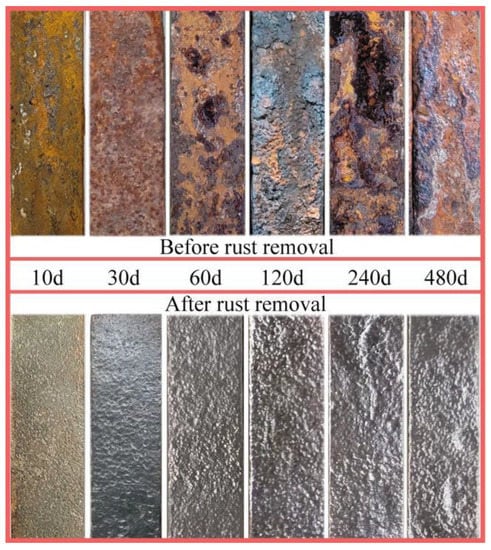
Figure 1.
Corroded steel plates.
2.2. Corroded Surface Measurement and Its Reconstructed Model
For evaluating the surface morphology and corrosion level of the specimens, the non-contact 3D scanner with an accuracy of 10 μm (produced by XTOM) was employed to measure the corroded surface of all specimens, as illustrated in Figure 2. The whole corroded surface of specimens was selected as the measuring region and the measurement step was selected by 50 μm.
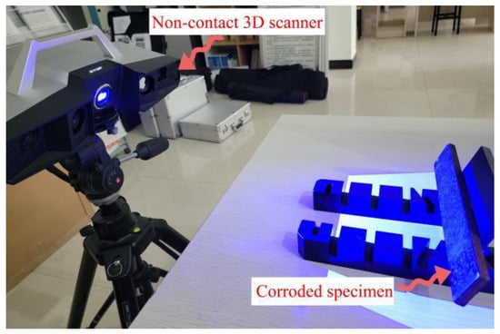
Figure 2.
Morphology measurement.
For the purpose of describing the corrosion results, the point cloud data obtained by the surface measurement were utilized as the 3D coordinate for reconstructing the corroded specimens. Firstly, the point cloud data were imported into Geomagic Studio for noise reduction and continuous treatment. Then, the treated data were imported into SURFER (a 3D scientific drawing software), and the reconstructed model of the specimens was established. Moreover, integer multiple square regions (ε × ε) were established on the whole reconstructed model surface along the length (x) and width (y) directions, as shown in Figure 3. Finally, a cube was constituted with each square and the average height () of its four corner points. If ε was small enough, the reconstructed surface was more consistent with the actual morphology, and the total volume of all cubes was believed to be closer to the volume of the specimen. Thus, the volume loss rate of the specimens (δDOPV) can be calculated by Equation (1).
where δDOPV is the volume loss rate of the specimen; Vinitial is the initial volume of the specimen, Vinitial = 16,000 mm3 in this work; m and n are the number of cubes along the width and length of the specimen; and is the mean value of the undulating profile in each square.
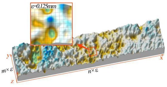
Figure 3.
The 3D model of corroded steel specimen.
The calculation value of δDOPV will converge with the decrease in ε; for defining the optimal size of ε, the specimen with 10 days of corrosion time was taken as an example, which was the most sensitive to ε because of its lowest amount of corrosion. Then, the ε was taken as 1 mm, 0.75 mm, 0.5 mm, 0.25 mm, 0.125 mm, and 0.075 mm, respectively, to reconstruct the corroded specimen, and the corresponding volume was calculated by using Equation (1). Figure 4 shows the relationship between the ε and δDOPV. As can be seen, δDOPV increases with the fineness of ε, and when ε = 0.25 mm, δDOPV tends to be stable. Therefore, the ε was regarded as 0.125 mm to reconstruct specimens, and Table 1 displays the value of δDOPV for all specimens.
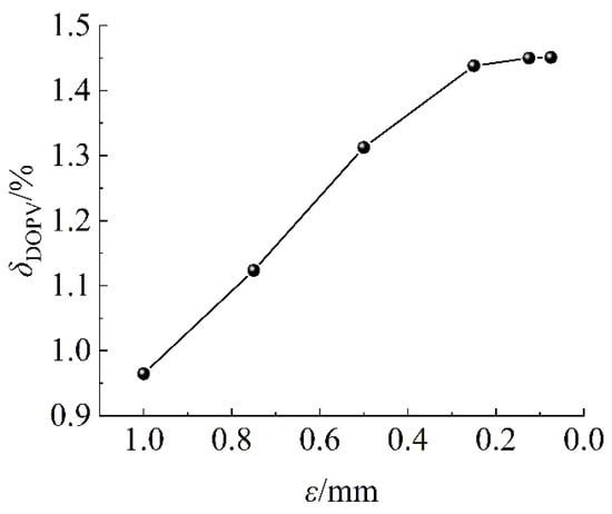
Figure 4.
Relationship between ε and δDOPV.

Table 1.
Calculated results of δDOPV of all corroded steel specimens.
2.3. Morphology Analysis of Corroded Surface
During the statistical analysis of the pitting parameters, due to the irregular shape of the corrosion pit, it is necessary to simplify the shape into a general three-dimensional geometric model. Based on this, the irregular corrosion pits were simplified to be semi-ellipsoid with certain pitting parameters (d, w and Rw/d), as shown in Figure 5.
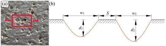
Figure 5.
Schematic diagram of pitting parameters: (a) corroded steel plate surface; (b) profile of the corrosion pit.
As the corrosion pit growth was a dynamic evolution process [29,30], the pitting parameters would be constantly changed. Thus, in every corrosion stage, the distribution law of the pitting parameters could always be used to describe the corrosion level of existing steel structures.
As for a corrosion pit, it is worth noting that since w was proportional to d [30], its scale can be fully described by a set of d and Rw/d, which can identify the size and shape of the pit. Therefore, the statistical analysis of the d and Rw/d for all specimens was operated, and the statistical results are illustrated in Figure 6.
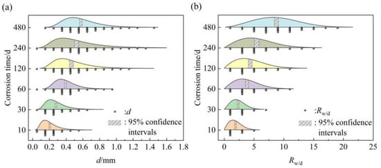
Figure 6.
Probability distribution of pitting parameters: (a) distribution of d; (b) distribution of Rw/d.
It can be clearly observed from Figure 6 that the size range of d and Rw/d expanded with the continuous corrosive attack. Based on the statistical results, although the specimens experienced different corrosion times, the distribution of d and Rw/d for all specimens revealed the same law, which follows the log-normal distribution. Its probability density function can be described by Equation (2).
where x is the log-normal random variable, which is the d and Rw/d in this work; μx and σx are the logarithmic mean value and standard deviation of the variable, respectively.
The statistical results of d and Rw/d of all specimens are summarized in Table 2. It can be seen that the logarithmic mean values of the statistical parameters (μd, μR) increased with corrosion degree, and there was no significant change in the standard deviation (σd, σR) between different corrosion levels. In addition, it is also apparent from this table that the maximum pitting damage (dmax and Rw/d, max) expanded with increased corrosion time. However, the dmin and Rw/d, min show an ambiguous regular change owing to the nucleation of new pits.
Table 2.
Statistical results of the pitting parameters.
Due to each pitting parameter following the log-normal distribution, the confidence interval of each pitting parameter can be used to evaluate the interval estimation, which reveals the comprehensive level of the corrosion pit on the specimen surface in each corrosion stage. Thus, the bootstrap method [34], available to calculate the confidence interval of skew distribution data, was adopted to obtain the 95% confidence interval of d and Rw/d for all specimens. The results are presented in Table 3.
Table 3.
Statistical results of 95% confidence interval of d and Rw/d.
As shown in 0, with increase in corrosion degree, the whole level of the 95% confidence interval of all pitting parameters gradually improved, which meant that the scale of the corrosion pits also expanded. However, the growth rate of d was obviously lower than that of Rw/d, inhere, d increased by about 2.85 times, whereas Rw/d grew approximately by a factor of 4.45. This phenomenon could be attributed to the accumulative effects of corrosion products and the passivation film on the corroded steel, which restricted the expansion of the corrosion pits in the longitudinal direction (pit depth direction). Meanwhile, the corrosion pits continue to expand laterally (pit width direction). As the corrosion pits expand, the adjacent corrosion pits are led to connect and merge, and then the corrosion pits with larger scale can be constantly formed. As a result of the combined influence of these factors, the corrosion pit gradually became wide and shallow with the increase in corrosion.
3. Modeling Method
3.1. Random Pitting Model (RPM)
As mentioned above, the distribution law of pitting parameters revealed the level of corrosion pits and the spatial variability of the corroded surface. Thus, to guarantee enough accuracy in simulating the corroded surface, it must ensure the similar distribution behaviors of each pitting parameter between the simulated corroded surface and the actual steel structure. Based on this, with the secondary development function of ABAQUS, the FEA model with random pitting surfaces can be created by establishing the constructor.
The secondary development aimed to constantly and automatically generate and randomly disperse corrosion pits whose scale complied with the distribution law of pitting parameters on the FEA model surface. Based on this, the constructors were established in Python scripting language, as illustrated in Equations (3) and (4).
where the dx and dy are the plane coordinate of the corrosion pit center; the L and W are the length and width of the simulated surface; the random.uniform is the random uniform distribution function in Python scripting language.
where the random.lognormal is the random lognormal distribution function in Python scripting language. Note that, to ensure that the scale of the corrosion pit on the simulated surface conforms to the statistical results, in the process of random corrosion pit generation, the d and Rw/d should be evaluated so that the d and Rw/d are always in the interval of [dmin, dmax] and [Rw/d, min, Rw/d, max], respectively.
The judgment of program termination is the key to stochastic modeling. In the actual modeling process, the corrosion degree can be used as the judgment standard of program termination. Currently, the evaluation criteria for the corrosion degree are mainly quantified by the mass loss rate (η), corrosion area loss rate (δDOP), and corrosion volume loss rate (δDOPV). Compared with δDOP, η and δDOPV have a more significant impact on the bearing capacity of corroded steel structures [35]. Thus, δDOPV was utilized as the control variable during the modeling, that is, once the volume loss rate of the FEA model (δ′DOPV) owing to the random corrosion pits was equal to the δDOPV of the specimens, the generation of the corrosion pits on the model surface was terminated. δ′DOPV can be obtained by Equation (5).
where Vi is the volume of the “i”th randomly distributed pitting pit; Vb is the initial volume of the FEA model; and k is the number of the corrosion pits generated.
After the value of parameters in the random pitting model (RPM), i.e., Equations (3)–(5) was determined, the FEA model of steel specimens with random pitting damage can be established according to the flow chart shown in Figure 7. Based on the statistical results of the pitting parameters and RPM, the simulated surface was generated, as shown in Figure 8.
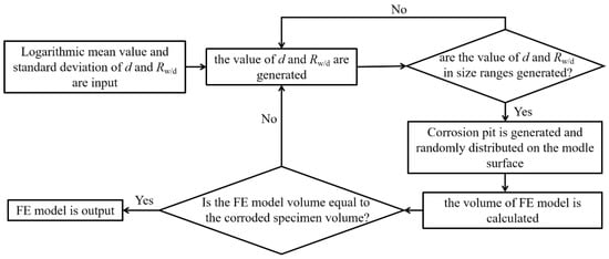
Figure 7.
Generation process of FEA model with random pitting damage.
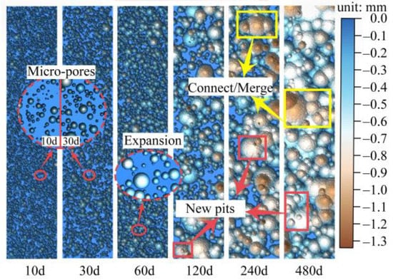
Figure 8.
Simulated corroded surface with different corrosion degrees.
It can be seen from Figure 8 that the morphological characteristics of the simulated surface based on surface measurements of a different corroded specimen were different. Moreover, the simulated surface also revealed a clear evolution law with the increase in corrosion time. At the early stage (10–30 d), the corrosion pits on the simulated surface were independently distributed as micro-pores. As the corrosion progressed (60–480 d), the corrosion pits continually expanded and connected with the adjacent pits. Additionally, the randomly formed pits created within the primary pits may likely reconstruct the secondary pit nucleation. The distribution of the pitting parameters of random pits on the surface of the FEA model was outputted to contrast with the statistical results (480 d), as shown in Figure 9.
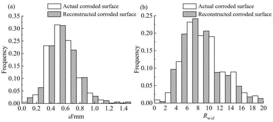
Figure 9.
Pitting parameter distributions of contrast simulated and actual surfaces: (a) statistical results of d; (b) statistical results of Rw/d.
As observed from Figure 9, the probability frequency distribution of the pitting parameters of the simulated surface was in good keeping with that of the actual corroded surface. Thus, the corroded surface simulated by the RPM can not only reproduce the complex evolution characteristics of the corrosion pit nucleation, connection, and overlap, but also the distribution law of the pitting parameters can be consistent with the actual situation.
3.2. Rough Surface Meshing Method (RSMM)
Optimizing mesh quality is another critical factor in improving the calculation accuracy and time of FEA, especially for models with a rough surface. Generally, it is difficult for FEA software to control the shape and number of elements. Thus, it is very necessary to require a meshing method for optimizing the FEA model with rough surfaces, i.e., corroded steel, in order to reduce the computing effort with sufficient accuracy. Compared with the tetrahedron element, the hexahedron element has obvious advantages in terms of calculation accuracy, deformation characteristics, number of element, and anti-distortion degree [36]. However, the model with the rough surface can only be smoothly meshed into tetrahedron elements in FEA software, resulting in an excessive number of elements, especially for large-scale corroded steel specimens. This could result in exorbitant computational costs. Thus, based on the method of reverse reconstruction, the rough surface meshing method (RSMM) was proposed, which can be implemented as follows:
(1) Establish the 3D solid model with random pitting damage in ABAQUS by using RPM.
(2) Convert the solid model into a shell model, which can be more easily and accurately meshed. Then, mesh the simulated surface to the appropriate size, and extract the 3D coordinate information of all elements of the simulated surface.
(3) Import the 3D coordinate information into the SURFER, which can process the 3D coordinate information with equal spacing, and build the boundaries of two sides of the corroded steel surface, as illustrated in Figure 10a.
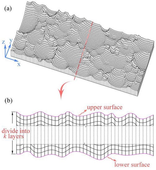
Figure 10.
Hexahedron element meshing method: (a) corroded surface after treatment; (b) cross-section of corroded steel in FEA model.
(4) Divide the distance between the z values of two sides at the same plane coordinate points (x, y) in equal proportion, so that the middle layer node can be obtained. Set up a series of elements layer by layer with eight nodes, as shown in Figure 10b.
The preceding procedures can be used to easily mesh the 3D FEA model with rough surfaces into hexahedron elements. In order to verify the effectiveness of RSMM, a steel plate (50 × 20 × 5 mm) was employed as an example, and the model was meshed by using the ABAQUS meshing module and the RSMM, respectively. The comparison results are shown in Figure 11.
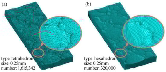
Figure 11.
Comparison of the element type: (a) tetrahedron element; (b) hexahedron element.
It can be observed from Figure 11 that, when the meshing size was the same (0.25 mm inhere), the RSMM can effectively reduce the number (by about 80%) and anti-distortion degree of elements for the same model while maintaining the local information of the simulated surface. Moreover, during the meshing process, the element size and element layers can be altered freely, allowing the number of elements to be adjusted according to the processing capability of the computer and the actual engineering needs.
4. Numerical Model Verification of Corroded Steel Beams
According to Ref. [37], the corroded surface morphology would tend to be stable when the measuring region of the corroded steel surface is greater than 20 × 20 mm2. Therefore, the overall surface characteristics of corroded steel structures can be reflected by morphological characteristics of its part surface zone. This also further proved that the distribution law of the pitting parameters obtained by the measurement region can be used for modeling larger corroded steel members.
In this work, the bending test of corroded steel beams in Ref. [8] was employed to verify the calculation accuracy of the FEA model established by applying the method proposed. The corroded steel beams used in the test were also obtained by an accelerated corrosion test, and their dimensions and corrosion degrees are shown in Figure 12 and Table 4, respectively.
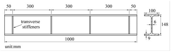
Figure 12.
Schematic diagram of steel beam section size.
Table 4.
Statistical table of steel beams corrosion rate.
As is well known, steel is a typical plastic material; the linear constitutive model used in FEA will inevitably change the deformation state of steel beams and reduce the calculation accuracy. So, a multi-linear kinematic hardening model was utilized in this work to be the constitutive model of corroded beams, as shown in Figure 13. As can be seen, this constitutive model comprised the entire elastic, yield, and strengthening phases, which were commensurate with the steel properties. Based on the test results in Ref. [8], the related parameters of the constitutive model in FEA were illustrated in Table 5.
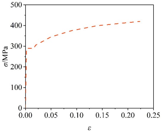
Figure 13.
Constitutive model of corroded steel.
Table 5.
Material Parameters of the FEA.
Three-dimensional solid elements, type C3D8R (8-node linear brick and reduced integration with hourglass control) were employed to model the corroded steel beam. This type of element demonstrates excellent ability for stress/displacement analyses. However, because the elements have only one integration point, it is possible for them to distort in such a way that the strains calculated at the integration point are all zero, which results in an uncontrolled distortion of the mesh. However, this can be solved by reasonably fining meshes, and can be minimized by distributing point loads and boundary conditions over a number of adjacent nodes [38]. Thus, the size effect of the element was also studied to determine a reasonable element size. The result was illustrated in Figure 14. Note that, the size of the FEA model’s surface element determined the accuracy of the simulated corroded surface, which also affected the calculation accuracy. Therefore, the surface element should be refined, and the horizontal axis in Figure 14 represents the surface element size.
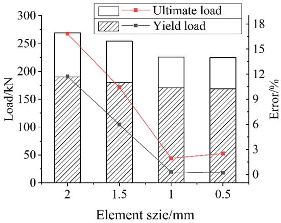
Figure 14.
Mesh convergence test.
It can be seen from Figure 14 that the calculation error decreased with the reducing of the element size. Apparently, while the element size was equal to 1 mm, the ultimate load and yield load calculation error converged. So, to reduce the calculation cost and improve its accuracy, the surface element size was refined to 1 mm, and the middle part with 2 mm element size. The boundary conditions of the model were consistent with the experimental conditions in the test, and the loads and boundary conditions were distributed to nodes at corresponding locations. The FEA model of the corroded beam is illustrated in Figure 15.
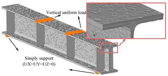
Figure 15.
FEA model of H-shaped steel beam with random corrosion pits.
To simplify the calculation, the following assumptions were made in the modeling process:
(1) The corroded steel beams were assumed as isotropy, so their η could be regarded as the δDOPV of it. Based on the value of δDOPV, the surface condition of the corroded beams could be appropriately connected with the specimens in this study during modeling: G1, G2—60 d; G3—120 d; G4—240 d; and G5, G6—480 d.
(2) It was assumed that the flanges and web had the same corrosion degrees, and the corrosion of the transverse stiffeners was not considered.
(3) The loading mode was displacement loading, which is easier to converge in FEA.
Figure 16 shows the FEA results of the corroded beam. As can be seen, the local buckling of the compressed flange and the bulging of the web occurred at the concentrated loading point, and the deformation becomes more obvious with the increase in corrosion degree. These deformation characteristics are consistent with those observed in the bending test [8]. Additionally, it is evident from Figure 16 that the stress distribution of corroded beams under various degrees of corrosion is different. Especially for the web, the high-stress area expanded with the corrosion degree. It is on account of that the evolution of corrosion pits causes the more complex corrosion morphology and larger scale of corrosion damage. Thus, it can be suggested that the characteristics of corrosion surfaces cannot be ignored in studying the mechanical properties of corroded steel structures.
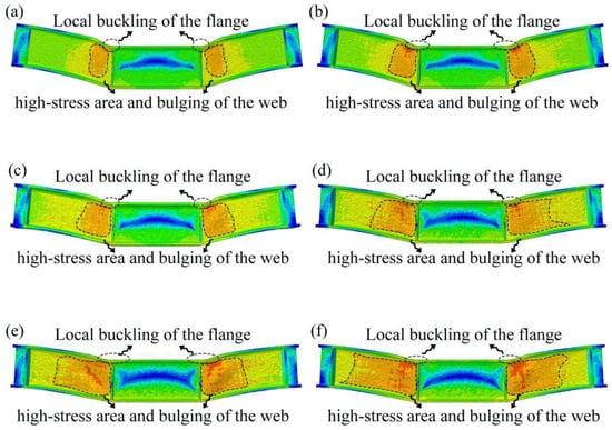
Figure 16.
Failure mode of corroded beam in FEA: (a) G1; (b) G2; (c) G3; (d) G4; (e) G5; and (f) G6.
The comparison of the load–midspan deflection curve between the calculation results and the test results is shown in Figure 17. Apparently, the load–midspan deflection curve of the FEA model agreed well with the test results. It is worth noting that, once the compressed flange buckled during the bending test, the load could not be continually increased [8]. Thus, to better verify the analysis accuracy, Fu of the FEA model was defined as the point at which buckling occurs during FEA.
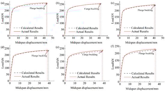
Figure 17.
Comparison of load displacement curves of simulated and test results: (a) G1; (b) G2; (c) G3; (d) G4; (e) G5; and (f) G6.
Further, the bearing capacities of the corroded beam, including the yield load (Fy), the ultimate load (Fu), the displacement corresponding to the yield load (∆y) and the displacement corresponding to the ultimate load (∆u), of the FEA results and the test results are shown in Table 6. It is apparent from this table that the maximum error of the bearing capacities between the FEA result and the test result is within 5%, which meets the engineering requirements. The present results confirm that the modeling method provided in this study could be well applied to investigate the mechanical properties of corroded steel structures.
Table 6.
Comparison of the numerical simulation results and the measured results.
5. Conclusions
The artificially accelerated corrosion test was carried out to obtain a batch of corroded steel specimens to investigate the distribution law of pitting parameters. Then, based on the statistical results of pitting parameters and the stochastic FEA method, the modeling and meshing methods for corroded steel structures were proposed. Finally, its calculation accuracy was verified by comparing it with the bending tests of the correlative corroded beams. The main conclusions are as follows:
(1) The pit depth (d) and the diameter–depth ratio (Rw/d) of corrosion pits on corroded steel surfaces obeyed the log-normal distribution. Furthermore, the corroded morphological characteristics and the corrosion pitting evolution were mainly determined by the wide–shallow corrosion pits. It was also proven by the change law of the confidence interval of d and Rw/d.
(2) The random pitting model (RPM), based on the statistical results of the pitting parameters and secondary development of ABAQUS, can be well used to simulate the FEA model of corroded steel structures. Moreover, the simulated surface reproduced a series of evolution characteristics of corrosion pit nucleation, growth, and connection with higher accuracy.
(3) The rough surface meshing method (RSMM) can be used to mesh the FEA model with an irregular surface into regular hexahedron elements. It cannot only reduce the number and distortion degree of elements, but also maintain the local information of the simulated surface. Additionally, the element number in the model can be easily adjusted by using the RSMM, and further to meet the accuracy requirements of the calculation results.
(4) By contrasting the bearing capacity of the corroded beam calculated by the FEA model with the test results, the comparison results show a less than 5% deviation between the FEA results and the test results for the bearing capacities of corroded steel beams. The provided modeling method with good reliability can be utilized further to study the mechanical properties of corroded steel structures in service.
Author Contributions
S.Z.: data curation, formal analysis, investigation, methodology, software, validation, and writing—original draft. S.G.: methodology and writing—original draft. S.R.: data curation, validation, and writing—original draft. Y.G.: validation and writing—original draft. C.K.: methodology and validation. L.Y.: methodology and writing—review and editing. All authors have read and agreed to the published version of the manuscript.
Funding
This research was funded by the National Natural Science Foundation of China, grant number: 51708467, the Doctoral Fund Project of SWUST, grant number: 16zx7136, and the Science and Technology Project of Sichuan Province, grant number: 2021JDZH0036.
Institutional Review Board Statement
Not applicable.
Informed Consent Statement
Not applicable.
Data Availability Statement
Not applicable.
Acknowledgments
The authors gratefully acknowledge the support provided by the National Natural Science Foundation of China (Grant No.: 51708467), the Doctoral Fund Project of SWUST (Grant No.: 16zx7136), and the Science and Technology Project of Sichuan Province (Grant No.: 2021JDZH0036). The authors also would like to express gratitude to the reviewers for their check and approve.
Conflicts of Interest
All authors of this manuscript directly participated in planning, execution, and analysis of this study. The contents of this manuscript are not copyrighted for publication previously. The contents of this manuscript are not now under consideration for publication elsewhere. The contents of this manuscript will not be copyrighted, submitted or published elsewhere while acceptance by Buildings. There are no directly related manuscripts or abstracts, published or unpublished, by any authors of this manuscript. We declare that, except “the National Natural Science Foundation of China” and “Doctoral Fund Project of SWUST”, we have no financial and personal relationships with other people or organizations that can inappropriately influence our work, there is no professional or other personal interest of any nature or kind in any product, service and company that could be construed as influencing the position presented in, or the review of, the manuscript entitled.
References
- Goto, Y.; Kawanishi, N. A unified analysis method to predict long-term mechanical performance of steel structures considering corrosion, repair and earthquake. In Advances in Steel Structures (ICASS ′02); Elsevier: Amsterdam, The Netherlands, 2002; Volume II, pp. 1145–1152. [Google Scholar] [CrossRef]
- Qin, S.; Cui, W. Effect of corrosion models on the time-dependent reliability of steel plated elements. Mar. Struct. 2003, 16, 15–34. [Google Scholar] [CrossRef]
- Melchers, R.E. Progress in developing realistic corrosion models. Struct. Infrastruct. Eng. 2018, 14, 843. [Google Scholar] [CrossRef]
- Yang, B.; Xiong, G.; Ding, K.; Nie, S.; Zhang, W.; Hu, Y.; Dai, G. Experimental and Numerical Studies on Lateral-Torsional Buckling of GJ Structural Steel Beams under a Concentrated Loading Condition. Int. J. Struct. Stab. Dyn. 2016, 16, 1640004. [Google Scholar] [CrossRef]
- Sheng, J.; Xia, J.; Ma, R. Experimental study on the coupling effect of sulfate corrosion and loading on the mechanical behavior of steel and H-section beam. Constr. Build. Mater. 2018, 189, 711–718. [Google Scholar] [CrossRef]
- Nie, B.; Xu, S.; Wang, Y. Time-dependent reliability analysis of corroded steel beam. KSCE J. Civ. Eng. 2019, 24, 255–265. [Google Scholar] [CrossRef]
- Wang, Y.; Shi, T.; Xu, S.; Niu, D. Experimental research and numerical analysis on the seismic performance of steel columns corroded in general atmospheric environment. China Civ. Eng. J. 2021, 54, 17. [Google Scholar]
- Sheng, J.; Xia, J.; Chang, H. Bending Behavior of Corroded H-Shaped Steel Beam in Underground Environment. Appl. Sci. 2021, 11, 938. [Google Scholar] [CrossRef]
- Wang, Y.; Zhou, X.; Wang, H.; Kong, D.; Xu, S. Stochastic constitutive model of structural steel based on random field of corrosion depth. Case Stud. Constr. Mater. 2022, 16, e00972. [Google Scholar] [CrossRef]
- Li, A.; Xun, S. Characterization of Surface Morphology of Neutral Salt-Spray Accelerated Corrosion Steel Structure by Fractal Dimension. Mater. Rep. 2019, 33, 6. [Google Scholar]
- Xun, S.; Li, H.; Wang, Y. Variation of multifractality of corroded steel surface with corrosion age. J. Harbin Inst. Technol. 2020, 52, 96–102. [Google Scholar]
- Songbo, R.; Ying, G.; Chao, K.; Song, G.; Shanhua, X.; Liqiong, Y. Effects of the corrosion pitting parameters on the mechanical properties of corroded steel. Constr. Build. Mater. 2021, 272, 121941. [Google Scholar] [CrossRef]
- Melchers, R.E. A Review of Trends for Corrosion Loss and Pit Depth in Longer-Term Exposures. Corros. Mater. Degrad. 2018, 1, 42–58. [Google Scholar] [CrossRef]
- Xu, S.; Mu, L.; Zhang, Z.; Li, R. Experimental study on flexural capacity of corroded cold-formed thin-walled C-section beams. J. Southeast Univ. (Nat. Sci. Ed.) 2021, 51, 7. [Google Scholar]
- Appuhamy, J.; Kaita, T.; Ohga, M.; Fujii, K. Prediction of residual strength of corroded tensile steel plates. Int. J. Steel Struct. 2011, 11, 65–79. [Google Scholar] [CrossRef]
- Li, A.; Xu, S.; Wang, Y.; Wu, C.; Nie, B. Fatigue behavior of corroded steel plates strengthened with CFRP plates. Constr. Build. Mater. 2022, 314, 125707. [Google Scholar] [CrossRef]
- Kainuma, S.; Jeong, Y.S.; Ahn, J.H. Investigation on the stress concentration effect at the corroded surface achieved by atmospheric exposure test. Mater. Sci. Eng. A 2014, 602, 89–97. [Google Scholar] [CrossRef]
- Xu, S.; Zhang, Z.; Qin, G. Three-dimensional Reconstruction and Degradation of Mechanical Properties Based on Real Surface of Corrosion Steel. J. Mater. Sci. Eng. 2017, 35, 6. [Google Scholar]
- Nakai, T.; Matsushita, H.; Yamamoto, N. Effect of pitting corrosion on strength of web plates subjected to patch loading. Thin-Walled Struct. 2006, 44, 10–19. [Google Scholar] [CrossRef]
- Nakai, T.; Matsushita, H.; Yamamoto, N. Effect of Pitting Corrosion on Ultimate Strength of Web Plates Subjected to Shear Loading. Key Eng. Mater. 2007, 340–341 Pt 1, 489–494. [Google Scholar] [CrossRef]
- Zhao, Z.; Zhang, H.; Xian, L.; Liu, H. Tensile strength of Q345 steel with random pitting corrosion based on numerical analysis. Thin-Walled Struct. 2020, 148, 106579. [Google Scholar] [CrossRef]
- Silva, J.E.; Garbatov, Y.; Soares, C.G. Ultimate strength assessment of rectangular steel plates subjected to a random localised corrosion degradation. Eng. Struct. 2013, 52, 295–305. [Google Scholar] [CrossRef]
- Silva, J.E.; Garbatov, Y.; Soares, C.G. Reliability assessment of a steel plate subjected to distributed and localized corrosion wastage. Eng. Struct. 2014, 59, 13–20. [Google Scholar] [CrossRef]
- Wang, R.; Shenoi, R.A. Experimental and numerical study on ultimate strength of steel tubular members with pitting corrosion damage. Mar. Struct. 2019, 64, 124–137. [Google Scholar] [CrossRef]
- Yuan, Y.; Zhang, N.; Liu, H.; Zhao, Z.; Fan, X.; Zhang, H. Influence of random pit corrosion on axial stiffness of thin-walled circular tubes. Structures 2020, 28, 2596–2604. [Google Scholar] [CrossRef]
- Zhao, Z.; Liu, H.; Liang, B. Assessment of the bending capacity of welded hollow spherical joints with pit corrosion. Thin-Walled Struct. 2018, 131, 274–285. [Google Scholar] [CrossRef]
- Wang, R.; Shenoi, R.A.; Sobey, A. Ultimate strength assessment of plated steel structures with random pitting corrosion damage. J. Constr. Steel Res. 2018, 143, 331–342. [Google Scholar] [CrossRef]
- Zhao, Z.; Tang, L.; Zhang, N.; Cai, Q.; Mo, S.; Liang, B. Shear capacity of H-shaped steel beam with randomly located pitting corrosion. Appl. Ocean. Res. 2021, 115, 102851. [Google Scholar] [CrossRef]
- Wang, H.; Xu, S.; Su, L. Statistical regularity of surface pitting morphology of steel in accelerated corrosion environment. J. Civ. Environ. Eng. 2016, 38, 7. [Google Scholar]
- Wang, Y.; Xu, S.; Li, H.; Zhang, H. Surface Characteristics and Stochastic Model of Corroded Structural Steel Under General Atmospheric Environment. Acta Metall. Sin. 2020, 56, 148–160. [Google Scholar]
- Zeng, S.; Ren, S.; Gu, S.; Gu, Y.; Kong, C.; Zhou, Q. Effects of Size Parameters of Stepwise Corrosion Pit on Stress Concentration of Steel and Its Computation Model Establishment. KSCE J. Civ. Eng. 2022, 26, 2813–2825. [Google Scholar] [CrossRef]
- Songbo, R.; Chao, K.; Ying, G.; Song, G.; Shenghui, Z.; Gang, L.; Tao, Y.; Yajie, Z. Measurement pitting morphology characteristic of corroded steel surface and fractal reconstruction model. Measurement 2022, 190, 110678. [Google Scholar] [CrossRef]
- GB/T 24517; Corrosion of Metals and Alloys-Outdoors Exposure Test Methods for Periodic Water Spray. China Standards Press: Beijing, China, 2009.
- Efron, B.; Tibshirani, R. Bootstrap Methods for Standard Errors, Confidence Intervals, and Other Measures of Statistical Accuracy. Stat. Sci. 1986, 1, 54–75. [Google Scholar] [CrossRef]
- Wang, R.; Fang, Y.; Dou, P.; Lin, Z. Investigation on ultimate strength of pile-foundation platform legs with pitting corrosion subjected to axial compression. Ocean. Eng. 2015, 33, 7. [Google Scholar]
- Bussler, M.; Ramesh, A. The eight-node hexahedral element in FEA of part designs. Foundry Manag. Technol. 1993, 121, 26–28. [Google Scholar]
- Liu, M. Accelerated Atmospheric Corrosion Simulation Test and Correlation Study. Master’s Thesis, AECC Beijing Institute of Aeronautical Materials, Beijing, China, 2003. [Google Scholar]
- Dassault Systemes, ABAQUS User Manual V. 6.14; Dassault Systemes: Vélizy-Villacoublay, France, 2014.
Publisher’s Note: MDPI stays neutral with regard to jurisdictional claims in published maps and institutional affiliations. |
© 2022 by the authors. Licensee MDPI, Basel, Switzerland. This article is an open access article distributed under the terms and conditions of the Creative Commons Attribution (CC BY) license (https://creativecommons.org/licenses/by/4.0/).