Article

A New Explication of Minimum Variable Sets (MVS) for Building Energy Prediction Based on Building Performance Database

1
School of Mechanical Engineering, Tongji University, Shanghai 200092, China
2
Sino-German College of Applied Sciences, Tongji University, Shanghai 200092, China
3
Tencent Technology (Shenzhen) Co., Ltd., Shenzhen 518054, China
*
Author to whom correspondence should be addressed.
Buildings 2022, 12(11), 1907; https://doi.org/10.3390/buildings12111907
Submission received: 18 July 2022 / Revised: 12 September 2022 / Accepted: 12 October 2022 / Published: 7 November 2022
(This article belongs to the Special Issue Building Performance Simulation)

Abstract

:
Building energy simulation plays a significant role in buildings, with applications such as building performance evaluation, retrofit decisions and the optimization of building operations. However, the wide range of model inputs has limited much research into empirically customized case studies due to the insufficient availability of data inputs or the lack of systematic feature selection of key inputs. To address this gap, this study proposes the concept of minimum variable sets (MVSs) for building energy-prediction models to improve the general applicability of building energy prediction using forward simulation. An MVS, in this paper, refers to a variable set that contains the most indispensable energy-related variables/features for annual building energy prediction. This study developed MVSs for office buildings by applying feature engineering algorithms to a Building Performance Database (BPD), which was established by integrating the design of experiments (DoE) method with high-dimensional data-space metrics, as well as parallel simulation. Supervised feature dimension reduction methods and multiple statistical criteria were adopted to choose different numbers of indispensable variables from the primary 16 building variables. The hierarchical MVSs that consist of the selected variables are characterized by the most influential features for building energy prediction, with certain requirements for prediction accuracy. To further improve the feasibility of MVSs, this study utilized two separate office buildings located in Shanghai and California as validation cases and provided comparable prediction accuracies across different sizes of MVS. The results showed that the MVS that has 12 variables has higher prediction accuracy than that which has 9 variables, followed by that which has 7 variables. Finally, the quantitatively hierarchical correlations between different sizes of MVS with different prediction accuracies for annual building energy could provide potential support for reasonable decision-making regarding building energy model variables, especially when comprehensive consideration is needed of the limited cost and data availability, and the acceptable accuracy of building energy.

1. Introduction

Generally, building energy-prediction models are classified into two basic categories: physical (or forward, white-box or classical) and data-driven (or inverse, statistical, black-box or machine learning) models [1,2,3,4]. Benefiting from the capability of solving the physical-description equations for the heat transfer of building and energy components [1,4], building simulation tools have become a most fundamental technique for creating buildings with energy-efficient design, energy-performance optimization and energy retrofit evaluation.
However, the issues of model reliability and universality have recently been broached since forward simulation models have been adopted in building energy-performance analysis. In this area, we can summarize the current applications of forward simulation in two ways: traditional forward modeling with building information, and the improved way of using a training-data-generation tool for data-driven models. Both of the above applications require high-quality parameterized inputs to produce convincing models. In traditional forward simulation, the physical modeling approach requires a physical description of the building design (e.g., geometry, envelope, internal gains and operational schedule), energy system (e.g., the type, capacity and thermal performance of kernel components) and local weather conditions as inputs to predict building energy use [5]. Excluding the assumptions that are made to reduce the complexity of the thermal mechanisms occurring in buildings, either inaccurate inputs or their uncertainties can result in poor prediction performance [6], and lead to real difficulty in evaluating the accuracy degree of the simulation models [1]. In the integrated application, various combinations of specific model inputs are simulated as hypothetical building cases, of which both the inputs and outputs are used as the training data for data-driven methods, such as regression models for building energy-consumption prediction [7], etc. Commonly, to ensure the robustness of the achieved data-driven models, the set of hypothetical building cases needs to cover a sufficient variety and diversity of building variables; however, there are too many input variables to be designed for hypothetical cases, which usually causes a large amount of simulation and time-consuming data-processing work. In this case, the shortage of current integrated application research is due to the models’ weak universality for other researchers due to the fact that the candidate variables to be designed are limited to a small range of building energy influential factors, to avoid extremely massive simulation [8,9,10]. As a consequence, concerns about the reliability or universality of building simulation models greatly eliminates the supportive potential of simulation models for building performance evaluation.
This study finds out the extent of the research gap. The discussion on the indispensable variables of building energy prediction will be crucial in taking full advantage of building simulation to encourage more efficient building energy-performance evaluation. If the wide range of building energy-related variables is not reasonably narrowed or systematically filtered in the above two kinds of application scenarios, either the interpretability or universality of the developed models will be questioned, especially under the circumstance of having limited data proof for the model inputs.
With the aim of supporting more persuasive and efficient building simulation, this paper targets the objective of building variables for energy prediction and explores the following two fundamental questions from the perspective of establishing more universal and referential methodology:
Q1.
Which building variables are the most indispensable for energy-prediction models?
Q2.
How do we achieve accurate building energy prediction with limited variables?
Recently, several researchers with experience of data analysis have gradually paid attention to the gap in feature selection for building energy-prediction models and have started to explore the model features/variables using feature engineering methods for machine learning. As summarized in Table 1, there are still some limitations in feature decision and selection in these building energy model studies. Firstly, the feature selection process is mostly designed for a specific building case with the aim of increasing the model performance and predicting its accuracy. The commonly used route is to apply a feature selection method to a pre-simulated [11] or measured [12] dataset of the target building, and then, to choose a set of important building/system variables for the preselected modeling method(s). In this case, the findings of the case studies resulted in the literature being too specific for the robust generalization of the built data-driven model [13]. Secondly, the primary features are determined by domain knowledge and data availability, which may just partially cover the influential variables, such as weather data [14,15], HVAC system [14], occupant behavior [16] or retrofit measures [13]. Moreover, different feature selection methods are rarely explored or discussed with consideration of their applicability and universality for the following model development.
Feature selection is regarded as a key data-preprocessing step in common machine learning. It has three main categories—the filter, wrapper and embedded/embedding methods [17,18,19]—that depend on how and when the utility of selected features is evaluated. Filter methods rely on analyzing the general characteristics of data and use suitable relevance metrics to measure the importance of candidate features, such as minimal redundancy–maximal relevance (MRMR) [19] and the principal component analysis (PCA) [20] method. The features chosen using filter methods are independent of the following machine learning algorithm [11,12]. Wrapper methods require a predetermined learning algorithm and use its performance on the provided features in the evaluation step to identify relevant features [11], such as recursive feature elimination (RFE) [15]. The embedded methods try to use the advantages of both wrappers and filters [21] and incorporate feature selection as a part of the model-fitting/training process, such as the application of a tree-based model algorithm [13,16]. Obviously, with the aim of establishing an accurate model, recent building energy model studies including feature selection processes have preferred to apply the wrapper and embedded methods, which result in higher learning performance for a particular learning model. Meanwhile, from the perspective of generalized applicability or statistical interpretability, the variables selected using the filter methods are relatively more universal to reflect the complex relationship between building factors and energy consumption, if there are sufficient data on building/system information and energy performance.
Table 1. Summary of building energy model studies focused on feature selection and analysis.
Case BuildingObjective Primary Features/Building VariablesObjective Building Prediction TargetFeature Selection MethodsPrediction Model MethodsDatabase Source for Prediction ModelReference
Office and campus buildings, U.S./ SpainWeather data, internal load, HVAC operation setpoint and time-lag variablesHourly cooling/heating energy consumptionFilter methods, wrapper methodsMultivariate adaptive regression splines/time-series modelSimulated data on an office building, and practical data on a campus building[11,12],
2019
Educational buildings, ItalyRetrofit intervention feature regarding building construction and HVAC systemWeekly building energy consumption for calculation of retrofit savings potential Wrapper feature selection, random forestHierarchical and k-medoids clustering, regression modelsEnergy Performance of Buildings (EPBD) platform by European Parliament 2012[13], 2019
Residential buildings, U.S.Building physics, weather data and occupant behaviorAnnual home energy consumptionRandom forest, principal component analysis-1000 Practical homes in Pecan Street Project 2010[16], 2018
Utility company and office building, ChinaWeather data, indoor environment and HVAC systemShort- and medium-term loadComparison of different subsets of primary variablesGaussian kernel regression model; nonparametric-based k-NN modelPractical data on two different locations (utility company and office building)[14], 2020
Commercial building, ChinaWeather data and timestampNext-day energy consumption and peak power demandRecursive feature eliminationEnsemble modelPractical data on a commercial building[15], 2014
Office building, ItalyWeather data, indoor environmental quality and HVAC equipment operationShort-term flowrate and energy consumption of heating systemGreedy randomized adaptive search procedure (hybrid filter–wrapper method)Autoregressive models with exogenous inputsPractical data on an office building[21], 2017
Generally speaking, the majority of building energy-prediction models with or without a feature selection step pay more attention to model performance, such as accuracy and practicability for the specific building(s), rather than the universality or generalization of their resulting models (including both selected variables and algorithms). Meanwhile, a convincing simulation/model for building energy-performance evaluation needs more reliable fundamentals on the complex relationship between influential inputs/variables and building energy consumption. To explore this gap, our study innovatively proposes the concept of minimum variable sets (MVSs), which contain the most indispensable variables for building energy prediction among full-scale building factors, along with their importance ranking and prioritization in building energy consumption.
This study has designed and developed an office BPD that only includes about 10,000 cases but can represent the high-dimensional space constituted by 16-D building variables. Hierarchical MVSs are then obtained by applying feature selection methods to this BPD. Furthermore, our research has determined the relationship between MVSs and the model’s predictive accuracy if using MVSs as model inputs, in the application of the resulting MVSs, to forward and data-driven models. Through the above research work, this paper attempts to answer the two mentioned questions, Q1 and Q2, and also provide a more universal and valuable reference for relevant research on input/variable selection in building energy-prediction models.
Relative to some existing research on building feature analysis, which mainly target the prediction accuracy of some specific data-driven models, this study makes the feature selection conclusion (such as MVSs) more compatible with and flexible to different kinds of building energy models, such as forward simulation. Based on the traditional application of supervised feature analysis algorithms, the construction method of MVSs takes consideration of hierarchical statistical criteria and feature rankings to increase its applicability for more convincing building simulation under insufficient-data conditions.
In this paper, the research framework and the key methods for MVSs are introduced in Section 2. Section 3 illustrates the application of the proposed methods for the development of the BPD and MVSs, with a discussion on the comparative analysis and key findings of hierarchical MVSs. Finally, the current study is concluded in Section 4.

2. Methods

Figure 1 illustrates the research framework of MVS study, including two main parts divided by the two questions, Q1 and Q2. The first part proposes a DoE method, called the hybrid space filling design, and the construction method of MVS. Using office building type as a pilot, this paper applies the proposed methods and establish hierarchical MVSs for the EUI prediction of office buildings to address question Q1. The second part validates the prediction accuracy of the hierarchical MVS, and determines the relationships among MVSs, the adopted feature selection criteria and the energy-prediction accuracy when using MVSs as model inputs. From the angle of answering question Q2, the hierarchical gradients of EUI prediction accuracy, achieved using different sizes of MVS, can provide potential support for reasonable decision-making in building energy model variables that are worthy of priority attention, especially when comprehensive consideration is needed of the limited cost and data availability, and the acceptable accuracy of building energy prediction, in most cases.
Within the research framework, the first part of the work on the Building Performance Database has been elaborated upon in our published paper [22], which will be simply summarized in this paper. This paper focuses on the construction, application, and validation of MVSs. The following is structured according to key steps of the framework in Figure 1. Section 2 provides the main research methods, including a simple introduction to the BPD, established using the hybrid space filling design method in Section 2.1 and the construction method of MVSs in Section 2.2. The application of the proposed methods, and the research results are presented and analyzed in Section 3. Section 3.1 provide the implementation results of the minimum variable sets construction method detailed in Section 2.2. The applications of the BPD are discussed in Section 3.2. Finally, conclusions are drawn in Section 4.

2.1. Introduction of Office BPD

As shown in Figure 1, the MVSs in this study are achieved by way of applying suitable feature dimension reduction methods (PCA and MRMR) to a pre-simulated medium-scale BPD, which is designed using a hybrid space filling design method, and then, simulated using EnergyPlus in batches.
The BPD is obviously a crucial part that has great impacts on the universality and flexibility of the achieved MVSs in this study. As the data basis for MVS construction, the BPD, which is more representative of the complex relationship between building/system factors and energy consumption, will make the achieved MVS more universal. It is required that the BPD covers the diversity of various energy-related building factors as much as possible, which means the DoE method should be efficient to ensure the fundamental function of the pre-simulated BPD in this study. The development of a BPD came from the idea of addressing the data-scarcity issue by way of big data in the area of building energy-prediction models. BPD establishment in the current research can be classified into three routes: direct massive simulation [23,24,25], the accumulated collection of measurements [26,27,28,29] or surveys [30,31,32]. Strictly speaking, the survey and measurement methods could be the first choices among the three mentioned routes of BPD construction to obtain practical building energy-performance data for the benchmark baseline definition and predictive model development, such as the commercial building energy-consumption survey (CBECS, 2018) [30], the residential energy-consumption survey (RECS, 2020) [33] the aggregated BEDES dataset (LBNL,2015) [27]. It is obviously that the needed time cost and platform resources for practical big data in the building sector are enormous for most research studies. Moreover, the key challenges come from the large-scale availability of building system characteristics data that are needed for broader applications but that are poorly achieved, as well as the “noise” of empirical data that limits the ability to extract decision-grade information [27]. Given this, many research studies take advantage of the forward simulation model and parameterization calculational tool to establish some targeted BPDs. A simulated BPD is commonly comprised of large-scale building cases, and each of them is identified with multiple building variables and the simulated building energy consumption. There are two types of pre-simulated BPD generation route. One way utilizes supercomputers and high-performance computing clusters (e.g., the Hopper system in [34]) to directly complete a huge amount of calculation without considering case-design methods to downscale the BPD. The other way applies some DoE or sampling methods to reduce the required number of cases, examining the whole design space, in which all the possible combinations are distributed evenly within the test range. The commonly used DoE methods for BPD establishment include orthogonal experiment design (OED) [35], the Monte Carlo (MC) method [7,8,9,10,11,12,13,14,15,16,17,18,19,20,21,22,23,24,25], and Latin Hypercube Sampling (LHS) [36]. As an important basis for building energy assessment and prediction, a useful BPD needs to cover as many possibilities as possible to ensure good performance of the trained model. The second way involves the selection of certain combinations of building factors to represent the full factorial space so that the corresponding computational expense is acceptable. Obviously, the second way is more efficient and practical, though it needs a statistically reasonable case design to ensure the representational capability of the built BPD.
Based on the above consideration, we have proposed the hybrid space filling design method for BPD establishment. This method of DoE combines the high-dimensional clustering method with existing statistical sampling methods to design a medium-sized BPD, summarized in Appendix A. Relative to some existing BPDs, the hybrid space filling design method makes the BPD construction more computationally efficient without the massive simulation cost of a supercomputer, and keeps the BPD more representative by covering variations in high-dimensional building variables. With this method, this study established an office BPD that only includes about 10,000 cases to represent the high-dimensional space constituted by 16-D building variables and the corresponding outputs (building energy consumption). The 16-D building variables are described in Table 2, including 12 numerical and 4 non-numerical variables. The other paper [22] published by the authors introduces the hybrid space filling design method and the BPD with details.

2.2. Construction Method of Minimum Variable Sets (MVSs)

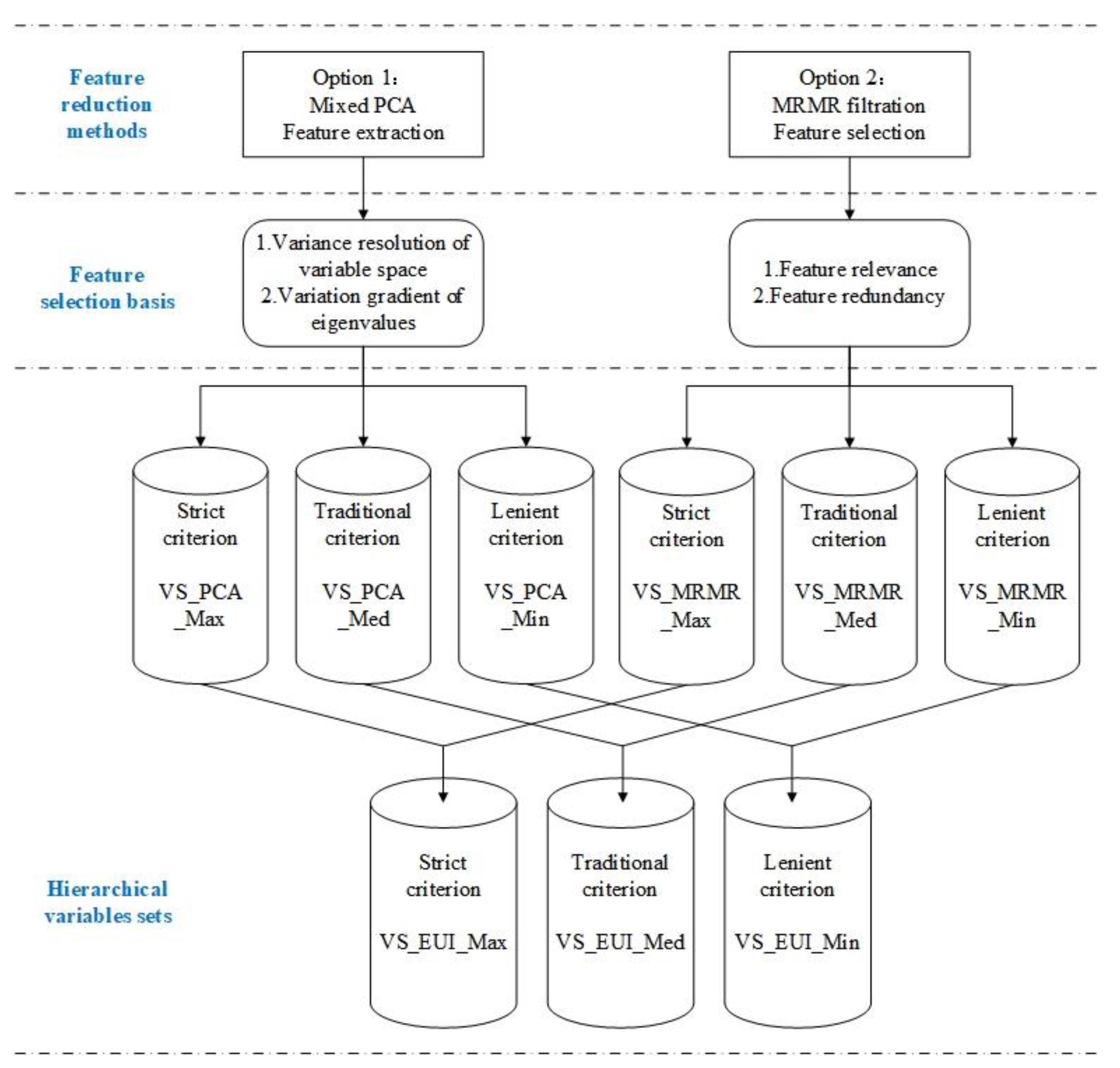
Supposing that a BPD using the hybrid space filling design is enabled to represent the complex relationship between high-dimensional variables and building energy consumption, the remaining work for answering Q1 should take full advantage of the BPD to explore the impacts of high-dimensional variables on building energy prediction and seek their rankings. This study utilizes two kinds of feature reduction method—principal component analysis (PCA) and max relevance–min redundancy filtration (MRMR)—on the pre-simulated BPD. The original concept of minimum variable sets (MVSs) is proposed on the basis of feature selection, which can statistically clarify the relationship between influential variables and building energy consumption and provide a quantitative comparison of the influential variables. Figure 2 illustrates the construction method of minimum variable sets, mainly including the application of both PCA and MRMR, and then, hierarchically, the combination of their feature selection results.
PCA is the most commonly used feature dimension reduction method in the category of feature extraction. Feature extraction usually maps the original high-dimensional space to a new space with lower dimensions. For an m-dimensional (m-D) space with n samples ( x i , 1 < i < n ), the mapping process of a data sample, x i , to the new lower-dimensional space is achieved via Equation (1), in which W refers to the new coordinates { w 1 , w 2 , ,   w d }, and each dimension of the low-dimensional coordinates is the linear combination of the original high-dimensional variables. The statistical principle of PCA requires a mapping process to ensure that the low-dimensional space can preserve the variability of the original high-dimensional space as much as possible. This requirement can keep the low-dimensional space informative about the high-dimensional space. Therefore, the performance of PCA is evaluated via the explanatory ability of the low-dimensional space on the original variance of high-dimensional variables, which is quantified by the ratio of the low-dimensional and high-dimensional variances. Based on the above, the mapping direction ( W ) is determined by maximizing the low-dimensional variance of the mapped samples, as shown in Equation (2). Through eigenvalue decomposition of the covariance matrix of the original m-dimensional data,   XX T , the PCA method utilizes the corresponding d eigenvectors of the top d eigenvalues as the mapping matrix, which is called the loading matrix. The loading matrix will be used as a d-dimensional linear transformation coefficient to map the primary X into the space of the active principal components (PCs), as shown in Equation (3).
x i = W T x i ,   d < m , W : w 1 = a 1 , a 2 , ,   a m w 2 = b 1 , b 2 , ,   b m w d = q 1 , q 2 , ,   q m
max W   t r W T X X T W ,   s . t .   W T W = I ,   XX T = i x i x i T
P C : P C 1 = w 1 X P C 2 = w 2 X P C d = w d X
In the PCA method, the dimensionality of the low-dimensional space, d, is a key factor and it will impact the explanatory performance of the variance of the original high-dimensional variables. A larger value of d means that more PCs are reserved and they can explain a larger ratio of original variance. Generally speaking, a threshold of 75~95% for the accumulative variance ratio is adequate [37]. In this study, we use gradient variance as the statistically quantitative criteria for PCA to achieve different number of PCs, which means different dimensionality of the low-dimensional space. In this way, the primary variables that are included in the selected PCs can constitute different sizes of minimum variable sets with a hierarchical number of indispensable building factors.
The other feature selection method we can see in Figure 2 is MRMR filtration, belonging to the category of filter selection. MRMR aims to directly select a subset of variables that have maximum relevance to the target variable (annual building energy consumption in this study), and the minimum redundancy among themselves at the same time [38]. The relevance between the building variables and the target variable (such as annual building energy consumption) reflects the contribution of each variable to building energy prediction, while the correlation between building variables reflects the similarities among them and can be used to exclude the redundant features. In this study, we use the Pearson correlation coefficient (PCC, see Equation (4)) algorithm to measure the statistical relativity of building variables and energy consumption. In Equation (4), the correlation coefficient,   ρ ξ , η , is the covariance of two variables, cov ξ , η , divided by the product of their standard deviation, var ξ and var η . Within the range of −1~1, when the absolute ρ ξ , η is closer to 1, the two variables are more relevant.
ρ ξ , η = cov ξ , η var ξ × var η
Similar to the settings for PCA application, different feature selection criteria are applied for MRMR, with gradient-filtering limitations of relevance and redundancy to obtain hierarchical MVSs. For example, this study will reserve the variables that have relevance to EUI of more than 0.05 and exclude the variables that have relevance with other variables of more than 0.5; these will be the VS_MRMR_Med set. Additionally, the VS_MRMR_Min set will be constructed by increasing the relevance threshold of EUI from 0.05 to 0.1, in order to remove the variables that are less relevant to EUI.
As shown in Figure 2, relative to the conventional application of a common feature analysis method with certain statistical criteria, the construction method of MVSs has two aspects of improvement. Firstly, quantitatively stratified criteria are adopted to select important variables in the application of feature reduction methods to the BPD. This study formulates three levels of statistical criteria— strict, traditional and lenient—for both the PCA and MRMR methods. PCA analysis usually ranks the variance explanatory proportions of several PCs, and each of the PCs is a linear combination of the original m-D variables. The PC ranking is then used to determine the number (d) of chosen PCs, with a pre-set ratio of the original m-D spatial variance that needs to be reserved by the lower d-D space. The MVS method uses the gradient levels of the pre-set ratio. For example, the requirement for a variance explanatory proportion of 70% will reserve the top 7 PCs, and one of 80% will reserve the top 9 PCs. Additionally, we utilize MRMR analysis to rank the m-D variables, sorted by their relevance to the target variable. Based on the MRMR ranking, different thresholds of PCC to EUI will choose different number of d-D variables. For example, the requirement for a PCC of more than 0.1 will reserve more top relevant variables than one of more than 0.05. Except for the relevance of each building factor to EUI, the MRMR method analyzes the correlations among all building variables. In the variable set chosen by the rank of their PCCs to EUI, if the PCC between any pair variables is more than 0.5, we recognize them as redundant variables to each other and could just choose one of them as an MVS. Secondly, the variable sets separately chosen using the PCA and MRMR methods are in union at each level, with the aim of preserving the statistical significance of the two methods.
Consequently, given the above quantitative criteria for feature selection, this study proposes a construction method for MVSs with the following three hierarchical levels:
  • Strict requirements include an accumulated variance contribution of 80% for the PCA method, and relevance of PCC to EUI of more than 0.05, with allowed redundancy among the chosen variables for the MRMR method. Strict criteria will achieve the largest size of MVS, VS_EUI_Max, and it is supposed to have the greatest capability for predicting building EUI.
  • Traditional requirements include an accumulated variance contribution of 80% for the PCA method, and relevance PCC to EUI of more than 0.05, without redundancy among the chosen variables for the MRMR method. Traditional critera will achieve a medium size of MVSs VS_EUI_Med, and it is supposed to have an acceptable capability for predicting building EUI.
  • Lenient requirements include an accumulated variance contribution of 70% for the PCA method, and relevance PCC to EUI of more than 0.1, without redundancy among the chosen variables for the MRMR method. Lenient criterion will achieve the smallest size of MVSs, VS_EUI_Min, and it is supposes to have an acceptable capability for predicting building EUI, especially for circumstances with some limitations in building or system information availability.
In our view, multiple options of MVSs with hierarchical sizes of energy-related variables could be more feasible and universal for building energy modelling research. To be a more quantitative and practical foundation for building energy model development, this paper attempts to bridge hierarchical MVSs with their predictive accuracy for building EUI. The way to achieve this is to separately use the selected variables, which belong to different MVSs, as the input parameters of the building energy models, and then, compare the predictive capabilities of the models with different numbers of input parameters. In this way, the hierarchical MVSs could be accompanied by the comparative accuracy for EUI prediction at each level, and they will be more supportive of the balance between the limited availability of building information and the accuracy acceptance of building energy prediction.
Obviously, the proposed method of MVS construction has ensured sufficient mathematical rationality and selected the most indispensable variables for building energy prediction with rankings of relevance to building EUI; however, there are issues of model integrity or model feasibility to be noted, especially for building forward simulation, if we use the variables that belong to the MVSs as model input parameters. As a mainstream method of building energy modeling, data-driven/inverse models can directly utilize the hierarchical MVSs thanks to their flexible model structure, without consideration of physical rationality. In that case, the smaller size of MVSs means fewer requirements of training data and fewer unknown parameters to be solved for a regression or an ANN model. As for forward simulation, for example, an EnergyPlus model requires complete model inputs to successfully run, due to the relatively fixed model structure and parameters. It is highly possible that the building model could not successfully run if we only input the parameters that belong to MVSs in the simulation model. Under the circumstances, this study utilizes the relevance ranks of building variables in MVSs as a valuable reference for simulation models.
Aiming to obtain quantitative reference for building energy-related variable selection for energy models, this study compares the predictive accuracy of different models (M1, M2 and M3) through the application of varying MVSs in the forward simulation models. With a well-calibrated model for an actual office building, M0 (as the baseline of comparative analysis), M1, M2 and M3 refer to the adjusted simulation models of the office building that separately apply hierarchical MVSs (VS_EUI_Max, VS_EUI_Med, and VS_EUI_Min) as their model inputs. These models are detailed as follows:
(a)
M0 is a calibrated model of an actual office building, complying with IPMVP (monthly errors of EUI of less than 10%). M0 is regarded as the baseline model for the accuracy analysis of M1, M2 and M3. The parameter values of the original m-D variables in the M0 model are regarded as the ground truth of the case building. The EUI calculated by M0 is named EUIB.
(b)
M1 is the 1st-version adjustment of M0, and the adjustment refers to the largest MVS1, VS_EUI_Max. If VS_EUI_Max has a number of important variables of d1, and d1 is no more than m, M1 keeps the values of the d1 parameters that belong to VS_EUI_Max the same as M0 and sets the values of the other parameters (number of m-d1) that are beyond the VS_EUI_Max default or the same as the ASHRAE guideline suggestions. The EUI calculated by M1 is named EUI1.
(c)
M2 is the 2nd-version adjustment of M0, and the adjustment refers to the medium size of MVS2, VS_EUI_Med. If VS_EUI_Med has a number of important variables of d2, and d2 is no more than d1, M2 keeps the values of the d2 parameters that belong to VS_EUI_Med the same as M0 and sets the values of the other parameters (number of m-d2) that are beyond the VS_EUI_Med default or the same as the ASHRAE guideline suggestions. The EUI calculated by M2 is named EUI2.
(d)
M3 is the 3rd-version adjustment of M0, and the adjustment refers to the smallest MVS3, VS_EUI_Min. If VS_EUI_Min has a number of important variables of d3, and d3 is no more than d2, M3 keeps the values of the d3 parameters that belong to VS_EUI_Min the same as M0 and sets the values of the other parameters (number of m-d3) that are beyond the VS_EUI_Min default or the same as the ASHRAE guideline suggestions. The EUI calculated by M3 is named EUI3.
Based on the above, the predictive capability of VS_EUI_Max, VS_EUI_Med and VS_EUI_Min could be formulated by the prediction error of EUIi (i = 1, 2, 3), relative to the baseline EUI0, as in Equation (5).
ε i = E U I i E U I 0 E U I 0 ,   i = 1 , 2 , 3
For an office building, M i   (i = 1, 2, 3) represents the building energy models with different fidelity degrees. The difference among M i models is the number of model input parameters that are matched with the actual building situation. Correspondingly, a different ε i illustrates an increase in model errors if the model fidelity decreases. Under the circumstance that building energy-related information is limited or time-consuming to acquire, the hierarchically quantitative relationship of M V S i , M i and ε i is able to support the decision of building model development. If the model is required to have an error of less than ε i for EUI prediction, this paper would suggest that the variables in M V S i should at least be matched with the actual building, like the model settings of M i . This would be applicable to guiding a building simulation on the fidelity requirements of important energy-related variables from masses of model input parameters, as well defining the boundaries of data acquisition, which is often time-consuming and without clear goals, but necessary to building energy simulation. In this way, the proposed MVSs provide quantitative support on building energy-related variable selection for building energy model development.

3. Results and Discussion

3.1. MVS for Office EUI Prediction

This section follows the MVS construction method (Figure 2) and establishes hierarchical MVSs. In the BPD, each case is illustrated using 16-D building variables and the corresponding building energy consumption, such as annual, sub-meter cooling/heating and daily energy consumption in the format of energy use intensity (EUI). Theoretically speaking, the method of minimum variable set construction is suitable for several statistics of building energy consumption, including annual, sub-meter cooling/heating and daily EUI, only if there is a representative dataset of high-dimensional building variables along with the corresponding EUI results. For the sake of clarity and brevity, this paper takes the MVSs for annual EUI as the applicant example in the results part.
Table 3 shows the hierarchical MVSs used for the annual EUI prediction of office buildings. From the original 16-D building variables, the MVS with the largest size chooses 13 variables as the necessary inputs for annual EUI prediction, called VS_EUI_Max. VS_EUI_Max is the set of the union of important variables chosen by the PCA and MRMR methods under strict statistical criteria, such as PCs that explain more than 80% of the variance and variables that have relevance to EUI of more than 0.05. The top 3 of the chosen 12 variables are the HVAC air-side system type (v13_HVAC), the plant type of energy system (v14_plant), and pump type (v15_trsp). They are followed by the variables related to local weather (v1_sat, v2_wat and v3_tat), building shape (v5_bsc), operation schedules (v16_schd), number of occupants (v9_ppd), window (v6_wwr), HVAC setpoint in summer (v11_sidt) and internal lighting power (v8_lpd). When it comes to the MVS of medium size, VS_EUI_Med, three variables (v14_plant, v15_trsp and v3_tat) are excluded from the above VS_EUI_Max, due to their redundancy to the reserved ones. v14_plant and v15_trsp are highly relevant to v13_HVAC, and the same situation occurs between v3_tat and v1_sat and v2_wat. So, VS_EUI_Med has nine variables, which are regarded as indispensable inputs for annual EUI prediction under the regular statistical criteria. Sequentially, the MVS with the smallest size removes the bottom two variables (v11_sidt and v8_lpd) from the VS_EUI_Med, and reserves the top seven important ones to form the VS_EUI_Min. It is noted that most of the variables selected using the two different methods (PCA and MRMR) are coincident at each level when we compare the importance rankings of the building variables for EUI prediction.
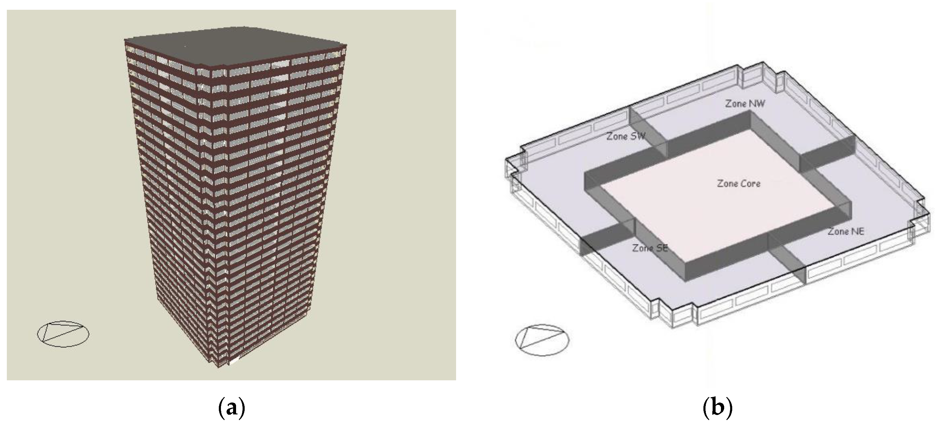
At the three levels of MVSs, VS_EUI_Max with 12 variables is supposed to have the highest predictive accuracy due to the fact that it has the largest coverage of building energy-related information. The accuracy of VS_EUI_Med and VS_EUI_Min is supposed to decline gradually. To quantitatively compare the predictive capabilities of MVSs of different sizes, this section follows the application method of MVSs in forward simulation (detailed in Section 2.2) by comparing the prediction errors ( ε i , i = 1, 2, 3) of models ( M i   , i = 1, 2, 3) for actual office building cases. Here, we utilized two EnergyPlus models of two actual office buildings located in Shanghai and California separately, as their own M 0 , after both of them were calibrated and met the verification requirements of IPMVP. The shapes of the two office buildings are attached in Appendix A. The results of M i and ε i indicate that, for the whole annual building EUI of the two cases, the prediction error ε 1 of M 1 , which uses VS_EUI_Max (12-D) as accurate model variables, is no more than 10%. The prediction error ε 2 of M 2 , which uses VS_EUI_Med (7-D), is no more than 15%. When it comes to the M 3 , which uses VS_EUI_Min (7-D), the error ε 3 increases to no more than 20%, as detailed in Table 3. The results demonstrate that the trend of the predictive accuracy of hierarchical MVSs quantitatively improves along with the increase in the included variables, and that the accuracy magnitude level of VS_EUI_Med can basically satisfy the requirement of annual EUI prediction. From the importance ranking of MVSs, we can conclude that, to predict annual EUI as accurately as possible, the priority order of the building variables that need to be matched to actual buildings is suggested to be HVAC system type, outdoor weather, building shape, operation schedule, occupants, envelope, etc., if there is limited data availability for all the building variables.

3.2. Application of the BPD

With the aim of providing a data basis for answering the two key questions in this study, an office BPD was designed and pre-simulated, including 9750 office building cases that have a variety of 16-D building energy-related features. Previous studies establishing BPDs have usually developed data-driven models with the BPD as the training data and regarded their models as an approximation of building simulation programs for their own research objectives, such as retrofit evaluation, technical baseline, etc. [24,30,32,34]. In addition to the application of the office BPD for MVS findings, this study also discusses the extrapolative application of the BPD from the simulation models to the approximate data-driven model. Here, as mentioned in the discussion part, the BPD was used as the training data for three Back-Propagation Artificial Neural Network models. The three BP models separately apply the hierarchical MVSs, VS_EUI_Max (12-D), VS_EUI_Med(9-D), and VS_EUI_Min(7-D), as their model variables, and the three models all aim to predict annual building energy consumption. So, we called the three BP models BP _ M 1 , BP _ M 2 and BP _ M 3 , according to the naming of M i in Section 3.2.
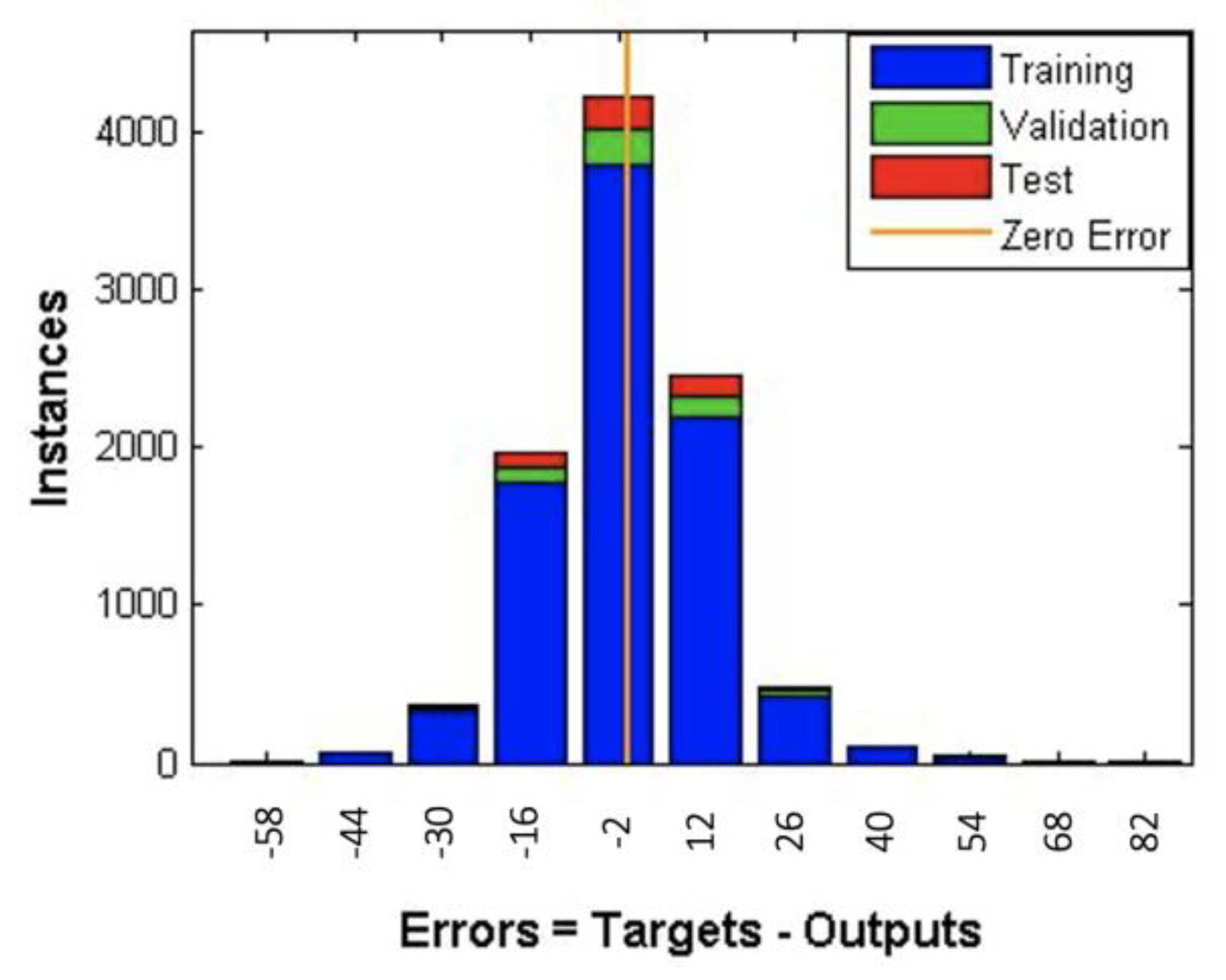
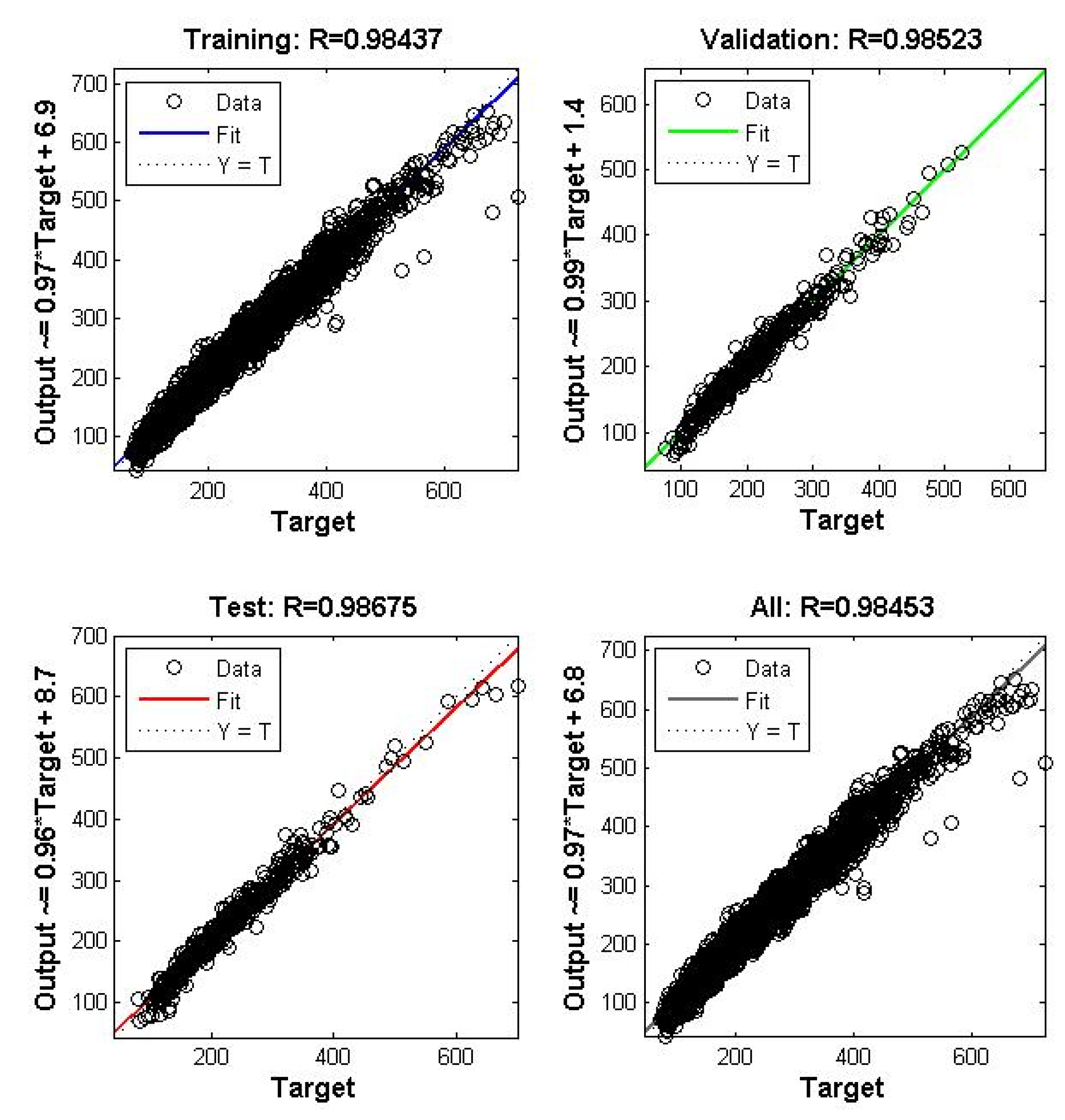
The BP ANN model is a commonly used data-driven algorithm for building energy prediction. For the sake of clarity and brevity, this paper explains the modeling process of BP _ M 1 as an example, and that the processes for BP _ M 2 and BP _ M 3 are similar. The settings of the BP model are listed in Table 4 and it is noted that the partitions of the BPD (9750 cases) for the training, validation and test are 90%, 5% and 5%. When the model iteration ends, the modeling results in Figure 3 imply that the absolute errors of the BP model show a normal distribution, and Figure 4 also shows good fit of the BP model to all of the training, validation and test sets, with high R values of more than 0.95.
Similar to the application of MVS from the perspective of forward simulation in Section 3.2, this study compares the prediction accuracies of the three models with different numbers of model input variables when they are used in actual office building cases. Table 5 provides the model errors of annual EUI prediction for the two buildings cases, and the results are analyzed based on several instances of BP modeling with the same settings, considering the random sampling of the training, validation and test datasets. Obviously, the comparative results of the BP model errors ( ε i ) also reflect the quantitatively increasing trend of the predictive accuracy of hierarchical MVSs, along with the increase in the included variables in the BP models. With the same BPD as the modeling dataset, the BP model with a larger number of input variables has higher fitting R and smaller ε i   o f   BP _ M i .
If we further compare the model accuracy of BP _ M i with that of M i , built in Section 3.2 for the same two actual offices. The errors of BP _ M i increase more prominently when the model variables are reduced from 12-D to 9- or 7-D than those of forward models M i . Using 12-D M V S 1 as the model variables, the errors of BP _ M 1 and M 1 are similar, and both of them are less than 10%. When the input variables of the BP models are reduced, the magnitude of model errors is obviously different for the two offices. For office 1 located in Shanghai, the effect of variable reduction in the BP models on predictive errors is close to that in the simulation models, due to the median ε i   o f   BP _ M i being within the range of ε i   o f   M i when i equals 2 or 3. Meanwhile, for office 2 located in California, the median ε i   o f   BP _ M i is obviously beyond the upper limit of ε i   o f   M i when i equals to 2 or 3. It seems that the predictive capability of the BP models is not stationary, and the BP models have worse predictive accuracy if the model variables are reduced, because the ε i   o f   t h e   forward   models   M i are smaller than the ε i   o f   BP _ M i , especially when using 9- or 7-D MVS as the model variables. This is reasonable because the forward   models   M i still have the impacts of the default settings of the excluded variables when the model variables are reduced from 12-D to 9- or 7-D, as described in Section 3.2, while the excluded variables are completely absent for the BP models.

4. Conclusions

Given that current building energy models lack reasonable feature selection in the area of forward simulation, this study aims to answer two fundamental questions about the indispensable variables for building energy prediction, to support more persuasive and efficient building simulation, especially with the limitation of data availability. With this goal, this study proposes a two-step framework of minimum variable sets (MVS), including BPD establishment first, and then, the development and estimation of hierarchical MVSs.
This study set out to gain a better understanding of the complex relationship between high-dimensional variables with building energy consumption. The rigorous design of the BPD basically ensures its representative capability, which is crucial for contributing some universal findings in the following MVS study. This paper first proposed the hybrid space filling design method for BPD establishment, and introduced high-dimensional space clustering to the commonly used random sampling method. With the efficient DoE plan, we establish an office BPD with 9750 office cases using parallel simulation. Each case is characterized by specific 16-D building variables, including basic building information, weather conditions, the building envelope, the internal load and the HVAC system, as well as the simulated energy consumption.
On the basis of the representative BPD, this study originally comes up with the concept of MVSs, which contain the most indispensable variables for building energy prediction with certain accuracy. The findings reported here shed new light on the quantitative relationships among the minimum variable set, the feature selection criteria and the model prediction accuracy. The strict feature selection criteria will achieve the largest size of MVS, and relatively, it has the highest accuracy of building EUI prediction. For example, VS_EUI_Max with 12-D variables is capable of contributing to the building energy model with a less than 10% error of annual EUI prediction. For the MVS with 9-D or 7-D variables, the model errors present an increase trend, along with a reduced number of indispensable variables.
These findings could provide a theoretical basis and data support for the appropriate trade-off of limited basic data and high requisition of office building energy prediction in practical applications. From the importance ranking of building variables in MVSs, we can conclude that, to predict annual EUI as accurately as possible, the priority order of building variables that need to be matched to actual buildings is suggested to be HVAC system type, outdoor weather, building shape, operation schedule, occupants, envelope, etc., if there is limited data availability for all the building variables.
This research offers a framework for the exploration of more convincing and efficient building simulation through a better understanding of the relationship between high-dimensional variables and building energy consumption. The key strengths of this study were the rigorous design of the BPD and the MVS concept, and their application method for building energy models. With regard to the research methods, some limitations need to be acknowledged. During the DoE of the BPD, two variables were simplified: building shape and usage schedules. For the building shape variable, the office building cases in the BPD only covered two common types of building shape: the square type and rectangle type. For building usage schedules, there were three scenarios to represent different operation situations, without consideration of the uncertainty of occupant behavior, to reduce the complexity of the DoE process. At the same time, with the limitation of the cost-consuming data collection of actual building cases, this study only checked the application of MVSs to two actual office buildings. With this study as a valuable framework trial, future work will cover more detailed model parameters for short-term prediction and utilize more practical building cases, and will extrapolate the methodology to other building types, as well.

Author Contributions

Conceptualization, M.Z., Y.P. and Z.H.; data curation, Y.L. and P.L.; funding acquisition, Y.P.; investigation, Y.L.; methodology, M.Z.; project administration, Y.P.; validation, Y.L.; writing—original draft, M.Z.; writing—review and editing, Y.P. All authors have read and agreed to the published version of the manuscript.

Funding

This study is supported by the National Natural Science Foundation of China (Grant No. 51978481).

Conflicts of Interest

The authors declare no conflict of interest.

Appendix A

Figure A1. Hybrid space filling design method for case design of BPD in [22].
Buildings 12 01907 g0a1
Figure A2. (a) Building shape and (b) floor layout of Case 1 (an office located in Shanghai, China).
Buildings 12 01907 g0a2
Figure A3. (a) Building shape and (b) floor layout of Case 2 (an office located in California, USA).
Buildings 12 01907 g0a3

References

  1. Foucquier, A.; Robert, S.; Suard, F.; Stéphan, L.; Jay, A. State of the art in building modelling and energy performances prediction: A review. Renew. Sustain. Energy Rev. 2013, 23, 272–288. [Google Scholar] [CrossRef] [Green Version]
  2. Zhang, Y.; O’Neill, Z.; Dong, B.; Augenbroe, G. Comparisons of inverse modeling approaches for predicting building energy performance. Build. Environ. 2015, 86, 177–190. [Google Scholar] [CrossRef]
  3. ASHRAE. 2013 ASHRAE Handbook—Fundamentals (SI Edition); American Society of Heating, Refrigerating and Air Conditioning Engineers (ASHRAE): Atlanta, GA, USA, 2013. [Google Scholar]
  4. Zeng, A.; Liu, S.; Yu, Y. Comparative study of data driven methods in building electricity use prediction. Energy Build. 2019, 194, 289–300. [Google Scholar] [CrossRef]
  5. ANSI/ASHRAE/IES Standard 90.1-2013; Energy Standard for Buildings Except Low-Rise Residential Buildings. ASHRAE Standard: Peachtree Corners, GA, USA, 2013.
  6. Amasyali, K.; El-Gohary, N.M. A review of data-driven building energy consumption prediction studies. Renew. Sustain. Energy Rev. 2018, 81, 1192–1205. [Google Scholar] [CrossRef]
  7. Amiri, S.S.; Mottahedi, M.; Asadi, S. Using multiple regression analysis to develop energy consumption indicators for commercial buildings in the U.S. Energy Build. 2015, 109, 209–216. [Google Scholar] [CrossRef]
  8. Wang, Z.; Wang, Y.; Srinivasan, R.S. A novel ensemble learning approach to support building energy use prediction. Energy Build. 2018, 159, 109–122. [Google Scholar] [CrossRef]
  9. Platon, R.; Dehkordi, V.R.; Martel, J. Hourly prediction of a building’s electricity consumption using case-based reasoning, artificial neural networks and principal component analysis. Energy Build. 2015, 92, 10–18. [Google Scholar] [CrossRef]
  10. Yan, L.; Liu, M. A simplified prediction model for energy use of air conditioner in residential buildings based on monitoring data from the cloud platform. Sustain. Cities Soc. 2020, 60, 102194. [Google Scholar] [CrossRef]
  11. Zhang, L.; Wen, J. A systematic feature selection procedure for short-term data-driven building energy forecasting model development. Energy Build. 2019, 183, 428–442. [Google Scholar] [CrossRef]
  12. González-Vidal, A.; Jiménez, F.; Gómez-Skarmeta, A.F. A methodology for energy multivariate time series forecasting in smart buildings based on feature selection. Energy Build. 2019, 196, 71–82. [Google Scholar] [CrossRef]
  13. Pistore, L.; Pernigotto, G.; Cappelletti, F.; Gasparella, A.; Romagnoni, P. A stepwise approach integrating feature selection, regression techniques and cluster analysis to identify primary retrofit interventions on large stocks of buildings. Sustain. Cities Soc. 2019, 47, 101438. [Google Scholar] [CrossRef]
  14. Ahmad, T.; Zhang, H. Novel deep supervised ML models with feature selection approach for large-scale utilities and buildings short and medium-term load requirement forecasts. Energy 2020, 209, 118477. [Google Scholar] [CrossRef]
  15. Fan, C.; Xiao, F.; Wang, S. Development of prediction models for next-day building energy consumption and peak power demand using data mining techniques. Appl. Energy 2014, 127, 1–10. [Google Scholar] [CrossRef]
  16. Zhang, C.; Cao, L.; Romagnoli, A. On the feature engineering of building energy data mining. Sustain. Cities Soc. 2018, 39, 508–518. [Google Scholar] [CrossRef]
  17. Iguyon, I.; Elisseeff, A. An introduction to variable and feature selection. J. Mach. Learn. Res. 2003, 3, 1157–1182. [Google Scholar] [CrossRef]
  18. Liu, H.; Motoda, H.; Setiono, R.; Zhao, Z. Feature Selection: An Ever Evolving Frontier in Data Mining. In Proceedings of the Workshop and Conference Proceedings 10: Fourth Workshop on Feature Selection in Data Mining, Hyderabad, India, 21 June 2010; Volume 10, pp. 4–13. [Google Scholar]
  19. János, V.Z.; Kis, K.B.; Fodor, Á.; Büki, Á.M. Adaptive, Hybrid Feature Selection (AHFS). Pattern Recognit. 2021, 116, 107932. [Google Scholar] [CrossRef]
  20. Odhiambo Omuya, E.; Onyango Okeyo, G.; Waema Kimwele, M. Feature Selection for Classification using Principal Component Analysis and Information Gain. Expert Syst. Appl. 2021, 174, 114765. [Google Scholar] [CrossRef]
  21. Antonucci, D.; Filippi Oberegger, U.F.; Pasut, W.; Gasparella, A. Building performance evaluation through a novel feature selection algorithm for automated arx model identification procedures. Energy Build. 2017, 150, 432–446. [Google Scholar] [CrossRef]
  22. Zhu, M.; Pan, Y.; Huang, Z. A Hybrid Space Filling Design Method of Building Performance Database Construction for Office. In Proceedings of the ASim 2018—4th Asia Conference of International Building Performance Simulation Association, Hong Kong, China, 3–5 December 2018. [Google Scholar]
  23. Zhao, J.; Plagge, R.; Ramos, N.M.M.; Simões, M.L.; Grunewald, J. Concept for development of stochastic databases for building performance simulation—A material database pilot project. Build. Environ. 2015, 84, 189–203. [Google Scholar] [CrossRef]
  24. Dipasquale, C.; Fedrizzi, R.; Bellini, A.; Gustafsson, M.; Ochs, F.; Bales, C. Database of energy, environmental and economic indicators of renovation packages for European residential buildings. Energy Build. 2019, 203, 109427. [Google Scholar] [CrossRef]
  25. Chen, Y.; Deng, Z.; Hong, T. Automatic and rapid calibration of urban building energy models by learning from energy performance database. Appl. Energy 2020, 277, 115584. [Google Scholar] [CrossRef]
  26. Gui, X.; Gou, Z. Association between green building certification level and post-occupancy performance: Database analysis of the National Australian Built Environment Rating System. Build. Environ. 2020, 179, 106971. [Google Scholar] [CrossRef]
  27. Mathew, P.A.; Dunn, L.N.; Sohn, M.D.; Mercado, A.; Custudio, C.; Walter, T. Big-data for building energy performance: Lessons from assembling a very large national database of building energy use. Appl. Energy 2015, 140, 85–93. [Google Scholar] [CrossRef] [Green Version]
  28. Kim, D.W.; Kim, Y.M.; Lee, S.E. Development of an energy benchmarking database based on cost-effective energy performance indicators: Case study on public buildings in South Korea. Energy Build. 2019, 191, 104–116. [Google Scholar] [CrossRef]
  29. Walter, T.; Sohn, M.D. A regression-based approach to estimating retrofit savings using the Building Performance Database. Appl. Energy 2016, 179, 996–1005. [Google Scholar] [CrossRef] [Green Version]
  30. U.S. Department Energy. Commercial Buildings Energy Consumption Survey. 2018. Available online: https://www.eia.gov/cbecs (accessed on 1 October 2022).
  31. Alstone, P.; Potter, J.; Piette, M.A. 2025 California Demand Response Potential Study—Charting California’s Demand Response Future: Final Report on Phase 2 Results; Lawrence Berkeley National Lab. (LBNL): Berkeley, CA, USA, 2017; Volume LBNL-20011.
  32. Yin, R.; Ghatikar, G.; Piette, M.A. Big-Data Analytics for Electric Grid and Demand-Side Management; Lawrence Berkeley National Lab. (LBNL): Berkeley, CA, USA, 2019.
  33. Berry, C.; Lawson, G.; Woodward, M. Highlights from the 2015 RECS: Energy Consumption, Expenditures, and End-Use Modeling; U.S. Energy Information Administration: Washington, DC, USA, 2018.
  34. Lee, S.H.; Hong, T.; Piette, M.A.; Sawaya, G.; Chen, Y.; Taylor-Lange, S.C. Accelerating the energy retrofit of commercial buildings using a database of energy efficiency performance. Energy 2015, 90, 738–747. [Google Scholar] [CrossRef] [Green Version]
  35. Mao, J.; Pan, Y.; Fu, Y. Towards fast energy performance evaluation: A pilot study for office buildings. Energy Build. 2016, 121, 104–113. [Google Scholar] [CrossRef]
  36. Kim, Y.J.; Yoon, S.H.; Park, C.S. Stochastic comparison between simplified energy calculation and dynamic simulation. Energy Build. 2013, 64, 332–342. [Google Scholar] [CrossRef]
  37. Li, W.; Huang, Y. A combined method of cross-correlation and PCA-based outlier algorithm for detecting structural damages on a jacket oil platform under random wave excitations. Appl. Ocean. Res. 2020, 102, 102301. [Google Scholar] [CrossRef]
  38. Peng, H.; Long, F.; Ding, C. Feature selection based on mutual information: Criteria of Max-Dependency, Max-Relevance, and Min-Redundancy. IEEE Trans. Pattern Anal. Mach. Intell. 2005, 27, 1226–1238. [Google Scholar] [CrossRef]
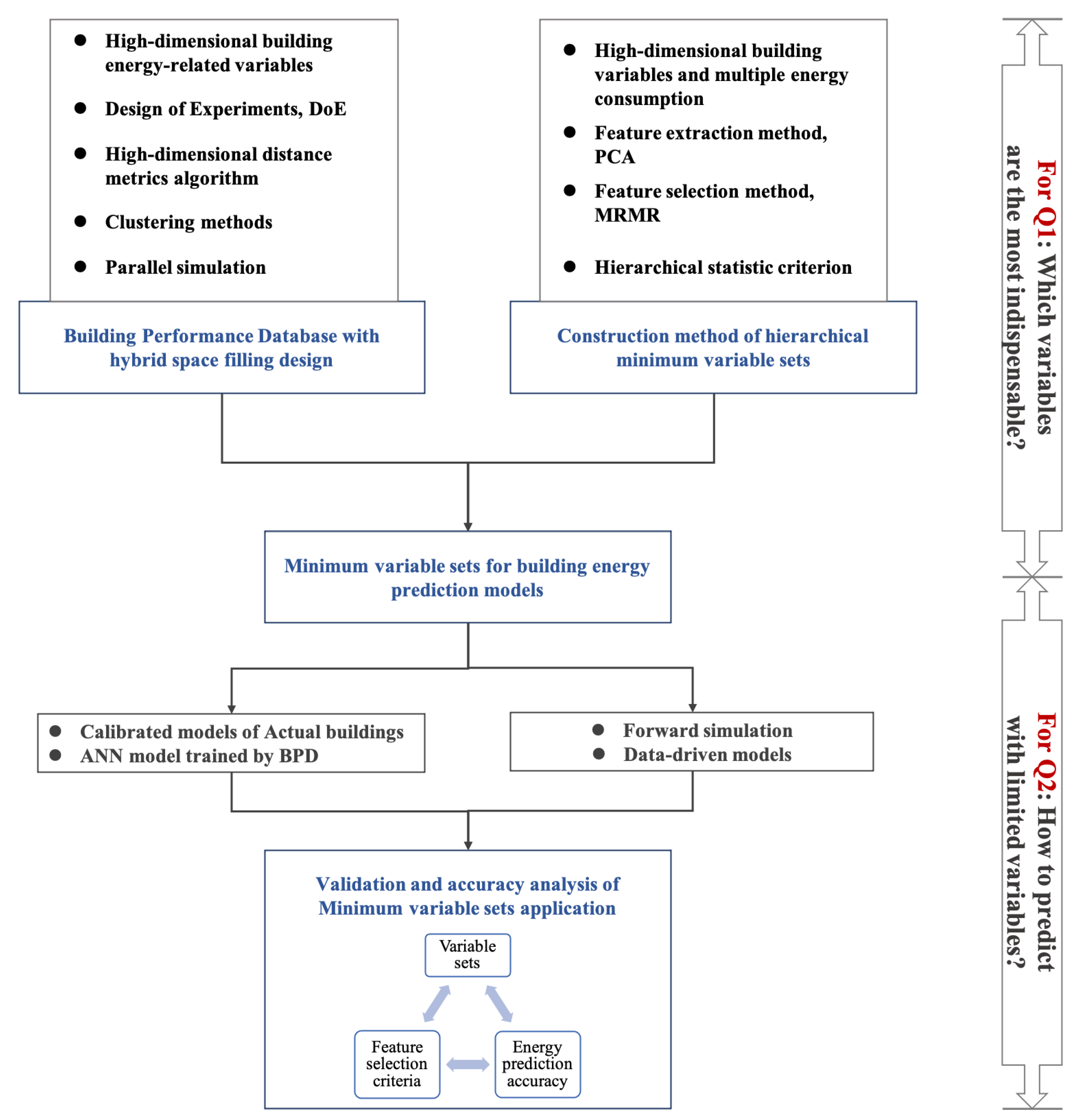
Figure 1. Research framework of minimum variable sets (MVS) for building energy-prediction models.
Buildings 12 01907 g001
Figure 2. The construction method of minimum variable sets (MVSs).
Buildings 12 01907 g002
Figure 3. Absolute errors of the developed BP ANN model.
Buildings 12 01907 g003
Figure 4. Fitting results of the developed BP ANN model for training, validation and test sets.
Buildings 12 01907 g004
Table 2. The 16-D variables covered by the office BPD.
Numerical Variable Description Range Non-Numerical Variable Description Range
v1_satSummer average temperature/°C16.0~31.0v13_HVACAll zones: CAVA0
v2_watWinter average temperature/°C−11.0~23.2All zones: VAVA1
v3_tatTransition average temperature/°C4.5~24.9All zones: FCU + OAA2
v4_sarhSummer average relative humidity0.28~0.88Core: VAV
Perimeter: FCU + OA
A3
v5_bscBuilding shape coefficient0.10~0.50All zones: VRVA4
v6_wwrWindow/wall ratio0.10~1.00v14_plantCentiChiller and boilerP0
v7_ohtcOverall heat transfer coefficient, OHTC, w/m25.0~35.0Screw chiller and boilerP1
v8_lpdLighting power density, w/m210.0~20.0Absorption chiller and boilerP2
v9_ppdPeople power density, m2/p2.0~10.0Ground-source heat pumpP3
v10_epdEquipment power density, w/m210.0~20.0Air-source heat pumpP4
v11_sidtSummer indoor design temperature/°C22.0~28.0CentiChiller and heat pump P5
v12_widtWinter indoor design temperature/°C15.0~22.0v15_tsptVariable speed pumpsY/N
v16_schdOperation schedulesHigh/Std/Low usage
Table 3. Minimum variable sets for annual EUI prediction.
MVS VS_EUI_MaxVS_EUI_MedVS_EUI_Min
Included variablesv13_HVAC
v14_plant
v15_trsp
v1_sat
v2_wat
v3_tat
v5_bsc
v16_schd
v9_ppd
v6_wwr
v11_sidt
v8_lpd
v13_HVAC
v1_sat
v2_wat
v5_bsc
v16_schd
v9_ppd
v6_wwr
v11_sidt
v8_lpd
v13_HVAC
v1_sat
v2_wat
v5_bsc
v16_schd
v9_ppd
v6_wwr
Variable number1297
ε i   o f   M i i = 1i = 2i = 3
6~9%8~11%14~17%
Table 4. Key settings of BP models.
Key SettingDescription
Training functionLevenberg–Marquardt BP algorithm
Hidden layer transfer/excitation functionsSigmoid function
Output layer transfer/excitation functionsLinear function
Number of nodes in hidden layer 2 n + 1 ,   in   which   n   equals   the   number   of   model   variables ,   such   as   12   for   BP _ M 1   and   9   for   BP _ M 2
Dataset partitionRandom sampling, with 90% (8774 cases) as training set, 5% (488 cases) as validation set, 5% (488 cases) as test set
Model evaluation index to end the trainingMean Square Error (MSE)
Table 5. Predictive error comparison of BP ANN models for actual offices.
Model Results of BP_Mii = 1i = 2i = 3
Model   variable   numbers ,   equal   to   M V S i 1297
Fitting   R   of   BP _ M i to training/test set0.95~0.980.82~0.870.82~0.85
ε i   o f   BP _ M i for office 1 in Shanghai1~11%9~15%13~24%
Median   ε i   o f   BP _ M i for office 1 in Shanghai5.8%8.9%15.0%
ε i   o f   BP _ M i for office 2 in California5~11%19~25%20~32%
Median   ε i   o f   BP _ M i for office 2 in California8.6%20.9%23.1%
Model results of
M i
6~9%8~11%14~17%
Publisher’s Note: MDPI stays neutral with regard to jurisdictional claims in published maps and institutional affiliations.