Laser Weld Aspect Optimization of Thin AISI 316 SS Using RSM in Relation with Welding Parameters and Sulfur Content

Abstract

A quantitative and qualitative study of the effect of laser (light amplification by stimulated emissions of radiation) welding parameters, such as focus point, welding speed, power beam and shield gas on bead profile in relation with microchemistry compositions differences of two thin AISI 316 industrial stainless steel casts have been studied. One cast contains 60 ppm (0.006%) of sulfur considered as high sulfur content and the other one contains 10 ppm (0.001 %) sulfur which can be considered as low sulfur content. A set of 27 tests were carried out by combining three welding speeds (1500, 3000, and 4500 mm/min), three shield gases (helium (He), mixture of 40% helium and 60% argon (Ar) and mixture of 70% helium and 30% argon) with flow rate of 15 L/min, and three focal lengths (+2, +7, and +12 mm). The depth, aspect ratio (the ratio between the penetration depth weld and the weld width) and the bead cross section profile are investigated using response surface methodology (RSM). Linear and quadratic polynomial models for predicting the weld bead geometry were developed. The results of the preliminary validation indicated that the proposed models predict the responses adequately. The geometry of the welded area was analyzed using optical microscopy, and correlations between weld morphology (depth, weld aspect parameter and weld area) and welding parameters were performed. For the cast 316 HS (high sulfur content), the main input factor influencing the depth weld (Y_d) is the focus point with a contribution up to 19.32. On the other hand, the main input factor affecting the depth weld (Y_d) of the cast 316 LS (low sulfur content) is the combination effect of focus point and power input energy with contribution up to 10.65%. Sulfur as the surfactant element contributes to determining the laser weld bead shape up to 71% when the welds are partially penetrated and diminishes to 50% when the welds are fully penetrated with the occurrence of the keyhole mechanism.

1. Introduction

Austenitic stainless steels are the most commonly used materials in heavy industries, especially in power generation, transportation, and petrochemical industry, due to their service performance, high weldability, and economical nature. They can be found in applications in which high-temperature oxidation resistance or high-temperature strength are required.

On the other hand, welding is widely used in several engineering applications, and many contemporary products, such as cars, transportation systems, and power plants [1,2].

Laser welding is extensively used in industry owing to its advantages of controlled heating, narrow weld bead and low heat affected zone (HAZ). In case of fully penetrated bead, laser welding has excellent characteristics with the equal sided fusion zone, lower heat input and distortion, improved welding surface finish, and lower residual stress in welds. Moreover, it has the ability to weld a wide range of metals and dissimilar metals [3,4]. Laser welding contributes to the renewal of production processes due to its ease, flexibility, high accuracy and high productivity. In fact, it is known to have many advantages compared to other welding methods [5,6].

There are different types of lasers, but the three widely used are neodymium-doped yttrium aluminum garnet (Nd:YAG), CO₂, and argon lasers [7]. Depending on laser power density and speed, the laser welding process can be either keyhole or conduction. In the conduction mode, the vaporization is minimal. Conduction-mode welds are produced using low-power laser beams and they are subsequently more shallower than keyhole-mode welds [8]. The material in the keyhole is rapidly melted and even boiled, thereby creating a metallic plasma around it. Boiling of the material maximizes the absorption of the material laser energy because it turns the keyhole to a black body [9].

Giudice Fabio et al. [10] used a heat conduction-based analytical model to simulate the thermal fields produced in high penetration laser beam welding. In this way, thermal profile and solidification mode can be investigated to predict the mechanical properties of laser joints. Pang [11] developed a three-dimensional computational fluid dynamics (CFD)-based model, incorporating coupled heat transfer, fluid flow and keyhole geometry. The author demonstrated that Marangoni convection enhances the heat transfer in molten pool.

Zhao et al. [12] studied the influence of heat transfer, mass transfer and liquid metal flow during stationary laser welding for different concentrations of oxygen in the surrounding environment. The authors found that the oxygen concentration affects not only the flow motion, but also the laser absorption coefficient. Having a clear understanding of the laser welding parameters that control the weld bead geometry is of interest to the industries. The microstructure and the mechanical properties are strongly affected by heat transfer and metal flow direction in the weld pool which are related to the presence or absence of the surfactant element.

Chan et al. [13] used nondimensional forms of the energy, continuity, and momentum equations and found that the highest fluid velocity and the solidification start position are at the edge of the beam due to the maximum temperature gradient at this point. In addition, the authors found that the width-to-depth ratio of the melt pool increases with the increase in Peclet number, and the increase in this ratio with the increase in the surface tension number was not uniform. Recently, Tomask [14] used a numerical simulation method to analyze stresses and cumulative plastic strain distributions. The author propose a modification of heat source models owing to the different power distributions and shapes of laser beams. A numerical approach was also conducted by Fabio Giudice et al. [15] to simulate and evaluate the thermal fields and cooling rates, the fusion zone composition and the solidification mode to predict the microstructure of the fully penetrated laser beam butt-welding of AISI 304 L plates with consumable insertion of AWS 308 L as filler material. The authors conclude that to avoid hot cracking, less filler metal must be added to the weld. Some works were performed to improve the performance of laser beam by using a set up for the coaxial combination of two laser beams to vary the intensity distribution [16], or by using hollow beam welding on bead-on-plate. Authors noted that when hollow beam welding is applied on 304 stainless steel sheets the spatters and the pores can be effectively suppressed, and the cooling rate during solidification process is increased and the austenite obtained is finer [17].

On the other hand, many studies [18,19] on laser welding parameters’ optimization have been carried out. For instance, Anawa et al. [20] used Taguchi methods and response surface methodology to study the effect of the process parameters, such as inert gas pressure, processing speed, laser power, beam incidence angle, and focal position on weld width, depth and area. Olabi et al. [21] used also Taguchi algorithms integrated approach to the optimization of CO₂ laser welding. They conclude that the laser power has a direct impact on weld geometries but laser focal position has less impact on weld pool geometry. On the other hand, it can contribute to increasing the weld area and weld width when its position is above the surface [21]. Many other authors investigated the optimization of the welding process parameters to achieve good weld profiles, such as Benyounis et al. [22] who adopted a statistical approach to correlate the welding parameters and the resulting weld profiles.

Moreover, the RSM is an increasingly popular method used to design experiment areas [23,24,25]. RSM design can optimize the expected properties through the setting of working parameters, such as laser beam power, welding speed, shield gas types as well as focus point. RSM can be used proficiently to get a mathematical modeling on output parameters, such as depth, aspect ratio and weld bead area while tuning the optimal input parameters.

The main aim of this study is to analyze the effect of the basic parameters of laser welding (i.e., laser beam power, welding speed, shield gas types as well as focus point) of plane plate of the 2.0 mm thick stainless steel AISI 316 sheets on the weld shape. RSM optimization method is used to develop a mathematical model on depth, aspect ratio and weld bead area in terms of welding parameters. The optimal response surface design is used to design the experiment. Using the optimal response surface design with 15 model points, 12 randomly selected points, and after performing the multi-regression analysis using the Design Expert software, the equations describing the relationship between the input parameters and the output are then obtained. In this study, Design Expert software is used to increase the model efficiency.

Based on the obtained results in this study, we will highlight the welding conditions which permit the surface-active elements to fully play their role. Moreover, the obtained results will enhance the understanding of the effect of laser welding parameters related to the surfactant elements, such as sulfur. These outcomes may help researchers as well as industries for improving the soundness of their products.

2. Materials and Methods

2.1. Material

Two casts of austenitic stainless steel, AISI 316 LS and AISI 316 HS, with thickness of 2 mm were investigated in this study. The chemical compositions, the temperature coefficient of surface tension and surface tension at melting temperature are presented in Table 1.

Table 1. Chemical composition (wt.%), the temperature coefficient of surface tension and surface tension at melting temperature of 316 stainless steel casts.

Elements	C	Mn	Si	P	S	Cr	Ni	Fe	γ (N/m) at Melting Temperature (1400 °C) [26]	d γ/dT (N/m K) [26]
316 HS SS	0.06	0.82	0.47	0.028	0.006	17.55	11.83	Balance	1.60	+10−4
316 LS SS	0.05	0.84	0.54	0.024	0.001	17.58	11.74	Balance	1.88	−10−4

Table 1 shows that the 316 LS has a negative temperature coefficient of surface tension (−10⁻⁴ N/m K). However, 316 HS tension surface is characterized by a positive temperature coefficient of surface tension (+10⁻⁴ N/m K)

During the welding process, a weld pool is formed when the base metal reaches its melting point with $\frac{\partial \gamma }{\partial T}$ negative, such as in the case of cast 316 LS, the molten metal flow outward (Marangoni convection) from the center to edges giving a wider bead with less depth penetration appears. Contrariwise, when $\frac{\partial \gamma }{\partial T }$ is positive, such as with cast 316 HS, the molten metal flow inward to the center of the weld pool (reverse Marangoni convection), leading to narrower and deeper weld bead.

2.2. Welding Procedure

The welding tests were carried out using a laser facility located at the central school of Nantes (France) with carbon dioxide laser capable of producing a maximum output of 6 Kw and emitting radiation in the infrared band of l0.6 μm and a pressure of 100 Pa. Figure 1 depicts focus point locations used during CO₂ laser beam welding experiments.

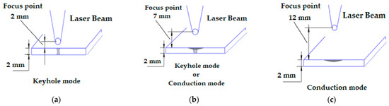
Figure 1. Scheme of a CO₂ laser beam focus position used: (a) focus point = 2 mm, (b) focus point = 7 mm, (c) focus point = 12 mm.

Using the RSM methodology with optimal response surface design that has 15 model points and 12 randomly selected points, a set of 27 tests were carried out by combining 3 welding speeds (1500, 3000, and 4500 mm/min), three shield gases (helium (He), mixture of 40% helium and 60% argon (Ar) and mixture of 70% helium and 30% argon) with flow rate of 15 L/min, and three focal lengths (+2, +7, and +12 mm), as depicted in Table 2. Table 3 shows the physical properties of the shield gases used. A preliminary study of the welding parameters is necessary to adjust the specific energy supplied to the sheets. Experiments consist of welding 120 mm line on a rectangular plate of 2 mm thickness, 150 mm length and 80 mm width. Before the welding operation, the plates were cleaned with acetone. During each test, three coupons were cut from the welding line to ensure the reproducibility and reliability of the results obtained. The results of the weld aspect (depth of penetration, width, and area) are depicted in Table 4; 11 represent an average of 3 readings. The samples were cut, polished and then etched by immersion in a solution composed of distilled water 190 mL, nitric acid 5 mL, hydrochloric 3 mL and acid hydrofluoric acid 2 mL for macrographic analysis.

Table 2. Laser welding parameters.

Exp. Number	Input Laser Welding Parameters				Linear Energy (J/cm)
	Focal (mm)	Speed (mm/min)	Power (w)	Shield Gas Gaz Proportion
	Xf	Xs	Xp	Xg
1	2	1500	3000	1:(70% He + 30% Ar)	120
2	2	3000	3000	1:(70% He + 30% Ar)	60
3	2	3000	5000	1:(70% He + 30% Ar)	100
4	2	4500	5000	1:(70% He + 30% Ar)	67
5	12	1500	3000	1:(70% He + 30% Ar)	120
6	12	3000	3000	1:(70% He + 30% Ar)	60
7	12	3000	5000	1:(70% He + 30% Ar)	100
8	12	4500	5000	1:(70% He + 30% Ar)	67
9	7	1500	3000	1:(70% He + 30% Ar)	120
10	7	3000	3000	1:(70% He + 30% Ar)	60
11	7	3000	5000	1:(70% He + 30% Ar)	100
12	7	4500	5000	1:(70% He + 30% Ar)	67
13	2	1500	3000	2:(100% He)	120
14	2	3000	3000	2:(100% He)	60
15	2	3000	5000	2:(100% He)	100
16	2	4500	5000	2:(100% He)	67
17	12	1500	3000	2:(100% He)	120
18	12	3000	3000	2:(100% He)	60
19	12	3000	5000	2:(100% He)	100
20	12	4500	5000	2:(100% He)	67
21	2	1500	300	3:(40% He + 60% Ar)	120
22	2	3000	3000	3:(40% He + 60% Ar)	60
23	2	3000	5000	3:(40% He + 60% Ar)	100
24	2	4500	5000	3:(40% He + 60% Ar)	67
25	12	1500	3000	3:(40% He + 60% Ar)	120
26	12	3000	3000	3:(40% He + 60% Ar)	60
27	12	4500	5000	3:(40% He + 60% Ar)	100

Table 3. Physical properties of the used shield gases.

Laser Welding Gas	Molecular Weight (g/mol)	Thermal Conductivity at 1 Bar, 15 °C (W/m K)	Ionization Energy (ev)	Dissociation Energy (ev)	Density Relative to Air
Helium	4	0.15363	24.6	0	0.14
Argon	40	0.01732	15.8	0	1.38

Table 4. The representation of the investigated factors and their corresponding responses (316 HS).

Exp. Number	Input Welding Parameters				Experimental Values
	Focal (mm)	Speed (mm/min)	Power (w)	Shield Gas	Weld Depth Penetration (mm)	Aspect Ratio	Area (mm2)
	Xf	Xs	Xp	Xg	Yd	Yr	Ya
1	2	1500	3000	1	2	3.42	74
2	2	3000	3000	1	2	1.73	45
3	2	3000	5000	1	2	1.42	63
4	2	4500	5000	1	2	1.63	55
5	12	1500	3000	1	0.6	0.42	15.5
6	12	3000	3000	1	0.35	0.27	7
7	12	3000	5000	1	0.62	0.74	34
8	12	4500	5000	1	0.44	0.33	11
9	7	1500	3000	1	2	1.58	86
10	7	3000	3000	1	1.15	0.98	25
11	7	3000	5000	1	2	1.19	79
12	7	4500	5000	1	1.09	0.65	32
13	2	1500	3000	2	2	2.9	78.5
14	2	3000	3000	2	2	2.43	49
15	2	3000	5000	2	2	2.24	51
16	2	4500	5000	2	2	2.86	42
17	12	1500	3000	2	0.44	0.25	14
18	12	3000	3000	2	0.38	0.26	10
19	12	3000	5000	2	1.12	0.7	36
20	12	4500	5000	2	0.72	0.52	16
21	2	1500	3000	3	1.98	3.31	70
22	2	3000	3000	3	0.65	2	40
23	2	3000	5000	3	0.49	0.25	9
24	2	4500	5000	3	0.91	2.3	47
25	12	1500	3000	3	0.8	0.71	12
26	12	3000	3000	3	0.48	0.41	8
27	12	4500	5000	3	0.44	1	10

2.3. Mathematical Modeling for 316 HS Cast

The regression analysis is used for developing a mathematical model of different output responses as function of the input parameters. After the preliminary investigation, a mathematical formulation based on a quadratic polynomial relation is established. The model can be classified as higher order polynomial relation. The choice of order two or three depends on the degree of fit that can be obtained. For 316 HS cast, satisfactory fitting results was obtained with two-order polynomial model. The quadratic function can be expressed as Equation (1) below.

$$Y=b_o+{\displaystyle \sum }_{i=1}^n{b}_i{X}_i+{\displaystyle \sum }_{j>i}^n{b}_{ij}{X}_i{X}_j+{\displaystyle \sum }_{i=1}^n{b}_{ii}{X}_i^2+\epsilon$$

(1)

where, X_i represents the four input factors such that i ∈ {f, s, p, g}, b represents the coefficient corresponding to the specified terms, b_o represents the constant term, b_i represents the coefficients of the linear terms, b_ij represents the coefficients of the linear interaction terms, b_ii represents the coefficients of the second-order (quadratic) terms, and ε is an error component.

By using the Design Expert software with a specified setting, the mathematical model for Y can be developed as a function of the input factors.

2.4. Mathematical Modeling for 316 LS Cast

The regression analysis is used for developing a mathematical model of the different output responses as a function of the input parameters. After the preliminary investigation, the adopted mathematical model involves a cubic polynomial relation. The cubic polynomial relation can be expressed as Equation (2) for 316 LS cast with or without data transformation. In fact, the model can be classified as higher order polynomial relation. For 316 LS cast, the satisfactory fit results were obtained with the three-order polynomial model. The model includes 35 terms. However, the only significant and mandatory terms will be considered.

$$Y=b_o+{\displaystyle \sum }_{i=1}^n{b}_i{X}_i+{\displaystyle \sum }_{j>i}^n{b}_{ij}{X}_i{X}_j+{\displaystyle \sum }_{i=1}^n{b}_{ii}{X}_i^2+{\displaystyle \sum }_{j>i}^n{{\displaystyle \sum }}_{k>j}^n{b}_{ijk}{X}_i{X}_j{X}_k++{\displaystyle \sum }_{j>i}^n{b}_{ijj}{X}_i{X}_j^2+{\displaystyle \sum }_{i=1}^n{b}_{iii}{X}_i^3+\epsilon$$

(2)

where, X_i represents the four input factors such that i ∈ {f, s, p, g}, b represents the coefficient corresponding to the specified terms, b_o represents the constant term, b_i represents the coefficients of the linear terms, b_ij represents the coefficients of the linear interaction terms, b_ii represents the coefficients of the second order terms, b_ijk represents the coefficients of the three factor interactions, b_ijj represents the coefficients of the interactions among the linear and the quadratic levels, b_ii represents the coefficients of the second order terms, b_iii represents the coefficients of the third order terms and ε is the error. As for the 316 HS cast, Design Expert software was used under a specific setting, where the mathematical model for Y can be identified as a function of the input factors.

3. Results and Discussions

3.1. Analysis and Discussions of 316 HS Cast

Figure 2 shows the macrographs of the laser welding carried out under a power of 5000 w, a speed welding of 3000 mm.min⁻¹, and a shield gas of (70% He + 30% Ar) for different focus points. We noticed that for a focus point at 12 mm far from the workpiece, the weld is partially penetrated, as depicted in Figure 2c. In this case, heat is absorbed from the laser beam over the top surface of the workpiece with heat losses to the environment, in spite of a consistent heat that is conveyed to workpiece. The heat required for fusion is provided from the surface by conduction and as a result, there is a low depth of penetration. At 7 mm focus point, the keyhole mode occurs, leading to a narrow and deep hole as shown in Figure 2b. In this case, plasma absorption does not occur and consequently, the heat is conveyed with high efficiency. On the other hand, the wide width at back side weld is ascribed to laser beam reflections occurred in keyhole. We can notice that the area section of the 7 mm weld bead (79 mm²) is higher than that of 2 mm focus point (63 mm²). At a focus point of 2 mm close to the workpiece, a plasma formation is expected to occur. Consequently, the interaction between the laser and the plasma vapor diminishes the total heat allowed for welding formation. Nevertheless, the remaining heat ensures a fully penetrated weld bead, as shown in Figure 2a. The keyhole geometry affects the weld geometry, such as width and depth.

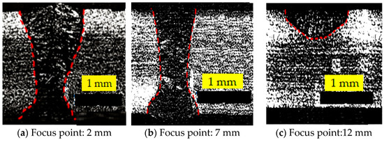
Figure 2. Effect of focus point on 316 HS laser weld carried out under power 5000 w, welding speed 3000 mm.min⁻¹, and shield gas (70% He + 30% Ar).

Table 4 shows the inputs, such as focus, speed, power, shield gas and experimental values, such as depth, ratio aspect and area used in this investigation. The results depict that the fully penetrated weld is achieved when the focus point is 2 mm and the shield gas of 100% He and with mixed shield gas (70% He + 30% Ar) are used regardless of the power provided or the chosen welding speed. The combination of high ionization energy and high thermal conductivity of helium gas make it the most efficient and common gas to be used for plasma control. Direct absorption of the laser beam in plasma is minimal with helium gas which ensures a good heat transfer to the workpiece. High thermal conductivity assures a cooling of the plasma and accordingly a reduction in plasma absorption. Furthermore, the aspect ratio and section area exhibited the highest values for welds carried out under 2 mm focus point and the shield gas of 100% He, or mixed shield gas (70% He + 30% Ar). Moreover, the weld bead depth, aspect ratio and weld section area decrease when the focal point is 7 mm. When the focus point is at 12 mm further away from the workpiece, the depth, aspect ratio and weld section become lesser. The highest linear energy of 120 J/cm ensures highest values of aspect ratio and weld sectional area. The molten metal in 316HS cast weld pool moves from the edges to the center, and the liquid metal flows in inward convection of the molten metal, called inverse Marangoni convection, leading to deeper and narrower weld bead [27]. Sulfur as the surfactant agent favorizes a full penetration.

3.1.1. Modeling of Weld Depth of Penetration (Y_d)

The response variable Y_d is modeled, as represented in Equation (3). For obtaining the best fit, the following setting was performed. The response Y_d was transformed using inverse square root transformation and, the quadratic model and auto-select of terms relying on the adjusted R² were adjusted.

$$\frac{1}{\sqrt{Y_d}}=0.5245-0.1163 {X_f}_{ }+3.29 \times {10}^{-04} X_s+8.4 \times {10}^{-05} X_p+0.2621 X_g+2.0 \times {10}^{-05} X_f{X}_s-3.30 \times {10}^{-05} X_f{X}_p+0.0909 X_f{X}_g-4.28 \times {10}^{-04} X_s{X}_g+0.0116 X_f²$$

(3)

Table 5 depicts the residuals calculation for the validation of the Y_d mathematical models. Residual results depict the validity and the accuracy of the Y_d mathematical model.

Table 5. Residues calculation for validation of the Y_d mathematical model.

Exp. Number	Xf	Xs	Xp	Xg	Yd	Transformed Value of Actual Yd $\frac{1}{\sqrt{{\mathit{Y}}_{\mathit{d}}}}$	Predicted Value	Residual
1	2	1500	3000	0.7	2	0.7071	0.8059	−0.0988
2	2	3000	3000	0.7	2	0.7071	0.7224	−0.0153
3	2	3000	5000	0.7	2	0.7071	0.7575	−0.0503
4	2	4500	5000	0.7	2	0.7071	1.05	−0.3425
5	12	1500	3000	0.7	0.6	1.29	1.21	0.0785
6	12	3000	3000	0.7	0.35	1.69	1.62	0.0727
7	12	3000	5000	0.7	0.62	1.27	1.199	−0.0710
8	12	4500	5000	0.7	0.44	1.51	1.4	0.1109
9	7	1500	3000	0.7	2	0.7071	0.7192	−0.0121
10	7	3000	3000	0.7	1.15	0.9325	0.9739	−0.0414
11	7	3000	5000	0.7	2	0.7071	0.6784	0.0287
12	7	4500	5000	0.7	1.09	0.9578	0.9331	0.0247
13	2	1500	3000	1	2	0.7071	0.7463	−0.0392
14	2	3000	3000	1	2	0.7071	0.6579	0.0492
15	2	3000	5000	1	2	0.7071	0.6929	0.0142
16	2	4500	5000	1	2	0.7071	0.6045	0.1026
17	12	1500	3000	1	0.44	1.51	1.43	0.0821
18	12	3000	3000	1	0.38	1.62	1.64	−0.0156
19	12	3000	5000	1	1.12	0.9449	1.01	−0.0668
20	12	4500	5000	1	0.72	1.18	1.22	−0.0456
21	2	1500	3000	0.6	1.98	0.7107	0.8258	−0.1151
22	2	3000	3000	0.6	0.65	1.24	0.9944	0.246
23	2	3000	5000	0.6	0.49	1.43	1.03	0.3992
24	2	4500	5000	0.6	0.91	1.05	1.2	−0.1497
25	12	1500	3000	0.6	0.8	1.12	1.14	−0.0235
26	12	3000	3000	0.6	0.48	1.44	1.61	−0.1675
27	12	4500	5000	0.6	0.44	1.51	1.45	0.0534

The significance of the proposed model can be noticed via the statistical parameters. Figure 3a shows the normal plot of residuals and Figure 3b the predicted transformed data against the actual transformed data. The normal plot of residuals depicts that the residuals (errors) are approximately normally distributed but there are three outliers. That means the errors are independent and random. Also, this distribution indicates the goodness of the regression model. The ANOVA results confirm the statistical significance of the proposed formulation, as listed in Table 6. The statistical indicators are as follows: F-value = 10.43, obtained R² = 0.8467, adjusted R² = 0.7656, and predicted R² = 0.6737. The values of the adjusted R² and the predicted R² indicate a reasonable agreement where the difference between them is small and is (less than 0.2) indicating the statistical significance of the equation. Moreover, the signal-to-noise ratio is sufficiently good, S/N = 10.1226 (values > 4 are considered good), which shows the adequacy of the model to represent the data.

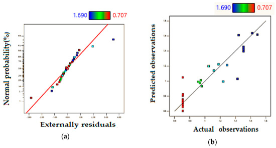
Figure 3. Model performance (a) normal plot of residuals, (b) predicted vs. actual observations for Y_d.

Table 6. ANOVA results of the Y_d in function of X_f, X_s, X_p and X_g.

Source	Sum of Squares	DF	Mean Square	F-Value	p-Value	Contribution (%)
Model	2.64	9	0.2935	10.43	<0.0001	11.80
Xf	0.4807	1	0.4807	17.09	0.0007	19.32
Xs	0.3025	1	0.3025	10.75	0.0044	12.16
Xp	0.3153	1	0.3153	11.21	0.0038	12.67
Xg	0.0086	1	0.0086	0.3046	0.5882	0.35
Xf Xs	0.1862	1	0.1862	6.62	0.0198	7.48
Xf Xp	0.3439	1	0.3439	12.23	0.0028	13.82
Xf Xg	0.134	1	0.134	4.76	0.0434	5.39
Xs Xg	0.1489	1	0.1489	5.29	0.0343	5.98
Xf ²	0.2743	1	0.2743	9.75	0.0062	11.03
Residual	0.4783	17	0.0281
Cor Total	3.12	26

Regarding the effect of the different terms of the equation on Y_d, the ANOVA results can be used to find the major factors that affect Y_d. (X_f) is the major factor which contributes to about 19.32% of the data variance with its linear effect. The quadratic effect of X_f is also significant; it contributes to about 11%. The second is the factor (X_p) whose linear effect comes with a percentage of 12.67% of the data variance. The third factor is X_s which contributes to about 12.16%. The linear effect of X_s is similar to the linear effect of X_p. The interaction effect between (X_f) and (X_p) gives it the second rank with a contribution of about 13.82%. This interaction effect can be noticed in Figure 4a. It is observed that both welding conditions have influence on the output variable (Y_a). The full depth penetration (2 mm) can be attained when X_p = 5000 W and X_p = 7 mm, but under a power of 5000 w, and a focus point close to the workpiece (2 mm) and when the formation of plasma prevent the efficiency of laser beam. However, if the focus point is at 12 mm far from the workpiece, the proportion of heat input is lost to surroundings. In addition, the interaction effect of (X_f) and (X_s) is significant and can be seen in Figure 4b. We can notice that under the used range of power, the full depth penetration (2 mm) can be attained when X_s = 3000 mm.cm⁻¹ and X_p = 7 mm. Using lesser speed welding can produce a collapsing of weld pool. In contrary, if the speed is higher, the heat provided is lesser leading to shallow weld penetration. Regarding the fourth parameter (X_g), its linear effect on Y_d is not significant where p-value > 0.05. However, the interaction effect of (X_s X_g) and (X_f X_g) are insignificant.

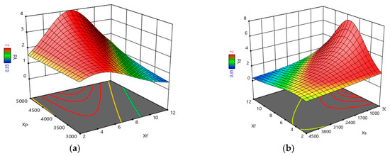
Figure 4. The effect of (a) X_f X_p and (b) X_f X_s on Y_d (3D).

3.1.2. Modeling of Weld Aspect Ratio (Y_r)

For the output response Y_r, the two factors interaction model without transformation gives the best fit. The obtained mathematical formulation for Y_r can be represented as Equation (4).

$$\sqrt{Y_r}=3.061-0.0952 X_f-5.51 \times {10}^{-04} X_p-0.7704 X_g+2.6 \times {10}^{-05} X_f{X}_p-0.107 X_f{X}_g+4.31 \times {10}^{-04} X_p{X}_g$$

(4)

Table 7 shows the residues calculation for validation of the Y_r mathematical models. It shows that the aspect ratio mathematical equations developed in terms of input parameters welding are well compatible with the actual output values.

Table 7. Residues calculation for validation of the Y_r mathematical model.

Exp. Number	Xf	Xs	Xp	Xg	Yr	$\mathbf{Transformed} \mathbf{Value} \mathbf{of} \mathbf{Actual} \left({\mathit{Y}}_{\mathit{r}}\right)=\sqrt{{\mathit{Y}}_{\mathit{r}}}$	Predicted Value	Residual
1	2	1500	3000	0.7	3.42	1.85	1.59	0.2602
2	2	300	3000	0.7	1.73	1.32	1.59	−0.2738
3	2	300	5000	0.7	1.42	1.19	1.19	−0.0025
4	2	4500	5000	0.7	1.63	1.28	1.19	0.0826
5	12	1500	3000	0.7	0.42	0.6481	0.6605	−0.0125
6	12	3000	3000	0.7	0.27	0.5196	0.6605	−0.1409
7	12	3000	5000	0.7	0.74	0.8602	0.7804	0.0798
8	12	4500	5000	0.7	0.33	0.5745	0.7804	−0.206
9	7	1500	3000	0.7	1.58	1.26	1.12	0.1322
10	7	3000	3000	0.7	0.98	0.9899	1.12	−0.1349
11	7	3000	5000	0.7	1.19	1.09	0.9873	0.1036
12	7	4500	5000	0.7	0.65	0.8062	0.9873	−0.1811
13	2	1500	3000	1	2.9	1.7	1.68	0.0208
14	2	3000	3000	1	2.43	1.56	1.68	−0.1232
15	2	3000	5000	1	2.24	1.5	1.55	−0.0493
16	2	4500	5000	1	2.86	1.69	1.55	0.1451
17	12	1500	3000	1	0.25	0.5	0.4325	0.0675
18	12	3000	3000	1	0.26	0.5099	0.4325	0.0774
19	12	3000	5000	1	0.7	0.8367	0.8113	0.0253
20	12	4500	5000	1	0.52	0.7211	0.8113	−0.0902
21	2	1500	3000	0.6	3.31	1.82	1.56	0.2612
22	2	3000	3000	0.6	2	1.41	1.56	−0.1439
23	2	3000	5000	0.6	0.25	0.5	1.08	−0.5769
24	2	4500	5000	0.6	2.3	1.52	1.08	0.4397
25	12	1500	3000	0.6	0.71	0.8426	0.7365	0.1061
26	12	3000	3000	0.6	0.41	0.6403	0.7365	−0.0962
27	12	4500	5000	0.6	1	1	0.7701	0.2299

The statistical analysis shows the satisfactory fitting level of the proposed model to represent the observed data. As shown in Figure 5a, the residuals are approximately around the line indicating that the errors are normally distributed; however, there is one outlier point. Moreover, Figure 5b shows a satisfactory distribution of the actual data against the predicted data. The ANOVA results for Y_r are listed in Table 8. As shown, the F-value = 12.86 is good with a p-value < 0.0001 which indicates that the proposed equation fits the measured data. The obtained R² = 0.7941, the adjusted R² = 0.7324, and the predicted R² = 0.6268 values can confirm the statistical significance of the mathematical model with an acceptable level. The signal-to-noise ratio, S/N = 10.74 > 4, indicates an adequate signal. Though this statistical analysis shows the proposed relation for predicting Y_r in function of the four parameters X_f, X_p, and X_g.

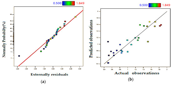
Figure 5. Model statistical indicators (a) normal plot of residuals and (b) predicted vs. actual observations for Y_r.

Table 8. ANOVA results of the Y_r in function of X_f, X_s, X_p and X_g.

Source	Sum of Squares	DF	Mean Square	F-Value	p-Value	Contribution (%)
Model	4.03	6	0.6714	12.86	<0.0001	14.02
Xf	3.38	1	3.38	64.69	<0.0001	70.60
Xp	0.0167	1	0.0167	0.3202	0.5778	0.35
Xg	0.0288	1	0.0288	0.5523	0.466	0.60
Xf Xp	0.3763	1	0.3763	7.21	0.0142	7.86
Xf Xg	0.1882	1	0.1882	3.6	0.0722	3.93
Xp Xg	0.1259	1	0.1259	2.41	0.1361	2.63
Residual	1.04	20	0.0522
Cor Total	5.07	26

Concerning the different terms of the equation, the ANOVA results show the statistical significance of the linear terms and the effect of their interactions. The factor X_f is responsible for the main effect which contributes to about 70.6% of the data variance. The second term is X_f X_p; it contributes to about 7.86% of the data variance. The effect of the other variables is small compared to X_f. The interaction relationship between X_f and X_g can be considered as significant with a confidence level of 90%; it contributes to 3.93% of the data variance. The interaction relationship between X_f and X_p can be illustrated in Figure 6a. One can remark that the maximum Y_r can be achieved when the focus point is 2 mm and the power is as less as possible (3000 w). The input variables X_f and X_p must be selected to avoid plasma formation and heat input losses. The interaction relationship between X_f and X_g can be illustrated in Figure 6b. It can be seen clearly that regardless of the focus point value, the shield gas 100% He is the best gas owing to its high thermal conductivity and ionization energy which ensures a good protection for the laser beam against plasma formation. The other terms represent X_p, X_g, and X_p X_g are considered as statistically insignificant since p-value > 0.1.

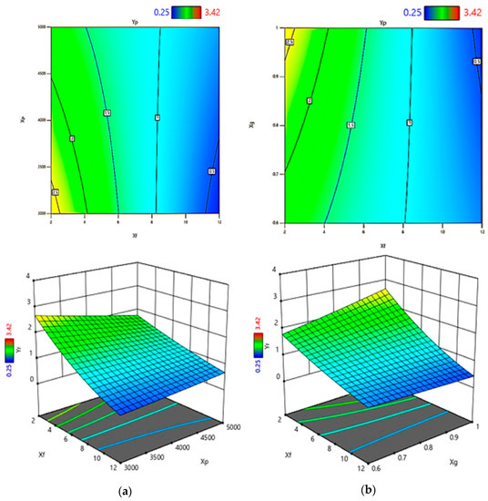
Figure 6. The effect of (a) X_f X_s (b) X_f X_g on Y_r (2D to 3D).

3.1.3. Modeling of Weld Bead Area (Y_a)

The response variable Y_a is modeled as represented in Equation (5). The response Y_a was transformed using inverse transformation. Furthermore, the quadratic model and auto-select of terms relying on the adjusted R² were adjusted. Table 9 shows the residues calculation for the validation of Y_a. The predicted values of Y_a are close to the actual values which indicates the strength of our optimization method.

$$\frac{1}{Y_a}=-1.73 \times {10}^{-03}-3.43 \times {10}^{-03} X_f+1.7 \times {10}^{-05} X_s+2.5 \times {10}^{-05} X_p-5.60 \times {10}^{-02} X_g+3.91 \times {10}^{-06} X_f \times X_s-5.66 \times {10}^{-06} X_f \times X_p+1.37 \times {10}^{-03} X_f²-5.11 \times {10}^{-09} X_s²$$

(5)

Table 9. Residues calculation for validation of the Y_a mathematical model.

Exp. Number	Xf	Xs	Xp	Xg	Ya	$\mathbf{Transformed} \mathbf{Value} \mathbf{of} \mathbf{Actual} \left({\mathit{Y}}_{\mathit{a}}\right)=\frac{1}{{\mathit{Y}}_{\mathit{a}}}$	Predicted Value	Residual
1	2	1500	3000	0.7	74	0.0135	0.0236	−0.0101
2	2	300	3000	0.7	45	0.0222	0.0052	0.017
3	2	300	5000	0.7	63	0.0159	0.0323	−0.0164
4	2	4500	5000	0.7	55	0.0182	0.0323	−0.0141
5	12	1500	3000	0.7	15.5	0.0645	0.0706	−0.0061
6	12	3000	3000	0.7	7	0.1429	0.1316	0.0112
7	12	3000	5000	0.7	34	0.0294	0.0455	−0.0161
8	12	4500	5000	0.7	11	0.0909	0.0835	0.0074
9	7	1500	3000	0.7	86	0.0116	0.0128	−0.0011
10	7	3000	3000	0.7	25	0.04	0.0444	−0.0044
11	7	3000	5000	0.7	79	0.0127	0.0149	−0.0022
12	7	4500	5000	0.7	32	0.0313	0.0235	0.0077
13	2	1500	3000	1	78.5	0.0127	0.0068	0.0059
14	2	3000	3000	1	49	0.0204	0.0091	0.0113
15	2	3000	5000	1	51	0.0196	0.0362	−0.0166
16	2	4500	5000	1	42	0.0238	0.0155	0.0083
17	12	1500	3000	1	14	0.0714	0.0538	0.0176
18	12	3000	3000	1	10	0.1	0.1148	−0.0148
19	12	3000	5000	1	36	0.0278	0.0287	−0.0009
20	12	4500	5000	1	16	0.0625	0.0667	−0.0042
21	2	1500	3000	0.6	70	0.0143	0.0292	−0.0149
22	2	3000	3000	0.6	40	0.025	0.0315	−0.0065
23	2	3000	5000	0.6	9	0.1111	0.0586	0.0525
24	2	4500	5000	0.6	47	0.0213	0.0379	−0.0166
25	12	1500	3000	0.6	12	0.0833	0.0762	0.0071
26	12	3000	3000	0.6	8	0.125	0.1372	−0.0122
27	12	4500	5000	0.6	10	0.1	0.0891	0.0109

The significance of the proposed model can be noticed via the statistical analysis. Figure 7a shows the normal plot of residuals and Figure 7b the predicted against the actual transformed data. The residuals are very closer and the line indicates that the errors are normally distributed; however, there is one outlier point As shown, the normal plot of residuals for depth Y_a is acceptable. In the same way, the predicted observations versus actual observations observation plot is satisfactory around the line. The ANOVA results confirm the statistical significance of the proposed formulation, as listed in Table 10. The statistical indicators are as follows: F-value = 13.12, R² = 0.8537, adjusted R² = 0.7886, and predicted R² = 0.6181. The values of the adjusted R² and the predicted R² indicate a reasonable agreement where the difference between them is small and less than 0.2, indicating the statistical significance of the equation. Moreover, the signal-to-noise ratio is sufficiently good since S/N = 12.427 which shows the adequacy of the model to represent the data.

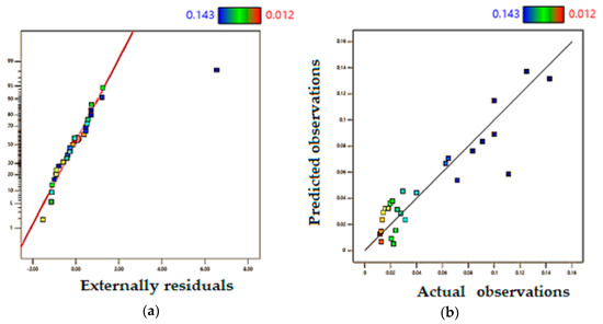
Figure 7. Model performance (a) normal plot of residuals and (b) predicted vs. actual observations for Y_a.

Table 10. ANOVA results of the Y_a in function of X_f, X_s, X_p and X_g.

Source	Sum of Squares	DF	Mean Square	F-Value	p-Value	Contribution (%)
Model	0.0356	8	0.0044	13.12	<0.0001	11.00
Xf	0.0024	1	0.0024	7	0.0165	6.00
Xs	0.0072	1	0.0072	21.3	0.0002	18.00
Xp	0.0029	1	0.0029	8.61	0.0089	7.25
Xg	0.002	1	0.002	5.93	0.0255	5.00
Xf Xs	0.0062	1	0.0062	18.39	0.0004	15.50
Xf Xp	0.0097	1	0.0097	28.75	<0.0001	24.25
Xf²	0.0038	1	0.0038	11.24	0.0035	9.50
Xs²	0.0014	1	0.0014	4.03	0.0601	3.50
Residual	0.0061	18	0.0003
Cor Total	0.0417	26

For investigating the significance of the different terms of the equation, the ANOVA results can be used to find the major factors that affect Y_a. After computing the percentage of contribution of each factor, the major contributor is the interaction of the two factors X_f and X_p. This interaction effect contributes to about 24.25% of the data variance and can be noticed in Figure 8a. Each of the input variables X_f and X_p, either separately or together influence the Y_a variable, and their interaction is crucial to avoid the metal vapors absorption by laser beam. The occurrence of this phenomenon would affect the efficiency of laser welding. The impact of the factor X_s on Y_a is significant; it represents the second major contribution with about 18%. The interaction effect of X_f and X_s is also significant and can be seen in Figure 8b and it is has the third major contribution with about 15.5%. The quadratic effect of X_f is also significant; it contributes to about 9.5%. The linear effect of the factors X_p, X_f, and X_g contribute 7.25%, 6.0%, and 5.0%, respectively, of the data variance. The quadratic effect of X_s is also significant; it contributes a small percentage of about 3.5%.

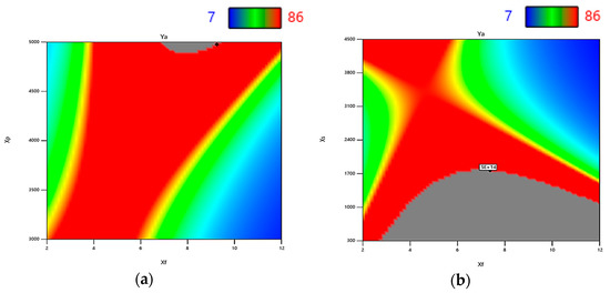
Figure 8. The effect of (a) X_f and X_p and (b) X_f and X_s on Y_a (2D).

3.2. Analysis and Discussions of 316 LS Cast

Figure 9 shows the micrographs of impact of focus point on 316 LS laser weld carried out under power 3000 w, speed welding 3000 mm.min⁻¹, shield gas (70% He + 30% Ar) for different focus points. One can notice that for focus points at 12 mm and 7 mm, the welds were partially penetrated, as depicted in Figure 9b,c. The heat required for fusion comes from the surface by conduction and as a result a low depth of penetration occurs. At 2 mm focus point, the keyhole mode occurs with a narrow and deep hole, as shown in Figure 9a.

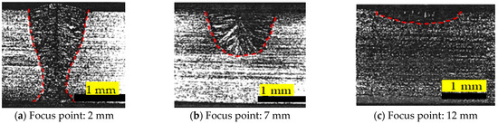
Figure 9. Effect of focus point on 316 LS laser weld carried out under power 3000 w, speed welding 3000 mm.min⁻¹, and shield gas (70% He + 30% Ar).

Table 11 depicts the input parameters and the output responses. The molten metal in 316 LS cast weld pool is governed by a surface tension-driven fluid flow in the weld pool. As the surface tension decreases with temperature, outward flow of the molten metal called Marangoni convection occurs, leading to wider and shallower weld bead [27]. The welds carried out with focus point 2 mm, and either the shield gas of 100% He or mixed shield gas (70% He + 30% Ar), were fully penetrated regardless of the power provided or welding speed chosen. It seems that the Marangoni is absent or hidden under 2 mm focus point close to the workpiece. The pressure of the vapor inside the keyhole contributes to the penetration by maintaining the keyhole, while the surface tension tends to retain it at the surface. It seems that the Marangoni convection contributes to laser bead shape at the focus points 7 mm, and 12 mm with mixed shield gas (40% He + 60% Ar) by decreasing the laser heat input to the workpiece.

Table 11. The representation of the investigated factors and the responses (Cast 316LS).

Exp. Number	Input Welding Parameters				Experimental Values
	Focal (mm)	Speed (mm/min)	Power (w)	Shield Gas	Weld Depth of Penetration (mm)	Aspect Ratio	Weld Area (mm2)
	Xf	Xs	Xp	Xg	Yd	Yr	Ya
1	2	1500	3000	1	2	2.52	67
2	2	3000	3000	1	2	2	55.5
3	2	3000	5000	1	2	2	48
4	2	4500	5000	1	2	2.31	46.5
5	12	1500	3000	1	0.39	0.2	12.5
6	12	3000	3000	1	0.29	0.18	8
7	12	3000	5000	1	0.48	0.23	17
8	12	4500	5000	1	0.61	0.43	15
9	7	1500	3000	1	2	1.89	98.5
10	7	3000	3000	1	0.93	0.76	24
11	7	3000	5000	1	2	2.5	68.5
12	7	4500	5000	1	1.08	0.58	39
13	2	1500	3000	2	2	2.9	73
14	2	3000	3000	2	2	2	47
15	2	3000	5000	2	2	2.4	50
16	2	4500	5000	2	2	2.53	47
17	12	1500	3000	2	0.74	0.51	18.5
18	12	3000	3000	2	0.28	0.18	8
19	12	3000	5000	2	1.04	0.62	28
20	12	4500	5000	2	0.53	0.38	13
21	2	1500	3000	3	0.63	0.34	11
22	2	3000	3000	3	2	1.7	50
23	2	3000	5000	3	0.18	0.08	4
24	2	4500	5000	3	0.61	0.27	8.6
25	12	1500	3000	3	0.77	0.57	17.9
26	12	3000	3000	3	0.5	1.09	9
27	12	4500	5000	3	0.6	0.49	12

3.2.1. Modeling of Weld Depth of Penetration (Y_d)

The response variable Y_d is modeled as represented in Equation (6). For obtaining the best fit, the following setting was performed. The response (Y_d) was transformed using the natural logarithmic transformation. The quadratic model and auto-select of terms relying on the adjusted R² were adjusted. Table 12 depicts the residuals calculation for validation of the Y_d mathematical models. The actual and predicted values of the depth matches well with the small differences between these values.

$$Ln \left(Y_d\right)=-10.8585+2.0928 {X_f}_{ }+5.8 \times {10}^{-5} {X_s}_{ }-3.12 \times {10}^{-3} X+33.7702 {X_g}_{ }-5.42 \times {10}^{-4} {X_f}_{X_s}+6.05 \times {10}^{-4} X_{f}X-6.3516 X_{f}X-3.32 \times {10}^{-7} X_{s}X+4.65 \times 10{-}^3 X_s X+3.36 \times {10}^{-3} X_{p}X-9.8 \times {10}^{-4} X_f²+2.65 \times {10}^{-7} X_s²-23.3712 X_g²+9.1 \times {10}^{-5} X_f X_{s}X-1.77 \times {10}^{-4} X_f{X}_{p}X+2.9 \times {10}^{-5} X_f² {X_s}_{ }-2.6 \times {10}^{-5} X_f² {X_p}_{ }+4.0420 X_f{X}_g²-4.2 \times {10}^{-3} X_s{X}_g²$$

(6)

Table 12. Residuals calculation for validation of the Y_d mathematical model.

Exp. Number	Xf	Xs	Xp	Xg	Yd	$\mathbf{Transformed} \mathbf{Actual} \mathbf{Value}=\mathit{L}\mathit{n} \left({\mathit{Y}}_{\mathit{d}}\right)$	Predicted Value	Residual
1	2	1500	3000	1	2	0.6931	0.5773	0.1159
2	2	3000	3000	1	2	0.6931	0.7046	−0.0114
3	2	3000	5000	1	2	0.6931	0.6899	0.0033
4	2	4500	5000	1	2	0.6931	0.8009	−0.1077
5	12	1500	3000	1	0.39	−0.9416	−0.9215	−0.0202
6	12	3000	3000	1	0.29	−1.24	−1.18	−0.0596
7	12	3000	5000	1	0.48	−0.734	−0.625	−0.109
8	12	4500	5000	1	0.61	−0.4943	−0.6831	0.1888
9	7	1500	3000	1	2	0.6931	0.7285	−0.0354
10	7	3000	3000	1	0.93	−0.0725	−0.0371	0.0354
11	7	3000	5000	1	2	0.6931	0.6578	0.0354
12	7	4500	5000	1	1.08	0.077	0.1124	−0.0354
13	2	1500	3000	2	2	0.6931	0.7689	−0.0758
14	2	3000	3000	2	2	0.6931	0.6435	0.0497
15	2	3000	5000	2	2	0.6931	0.6435	0.0497
16	2	4500	5000	2	2	0.6931	0.7167	−0.0236
17	12	1500	3000	2	0.74	−0.3011	−0.352	0.0509
18	12	3000	3000	2	0.28	−1.27	−1.24	−0.0309
19	12	3000	5000	2	1.04	0.0392	0.0578	−0.0186
20	12	4500	5000	2	0.53	−0.6349	−0.6335	−0.0014
21	2	1500	3000	3	0.63	−0.462	−0.3503	−0.1117
22	2	3000	3000	3	2	0.6931	0.6598	0.0334
23	2	3000	5000	3	0.18	−1.71	−1.75	0.0334
24	2	4500	5000	3	0.61	−0.4943	−0.5393	0.045
25	12	1500	3000	3	0.77	−0.2614	−0.3582	0.0968
26	12	3000	3000	3	0.5	−0.6931	−0.6561	−0.037
27	12	4500	5000	3	0.6	−0.5108	−0.451	−0.0598

The significance of the proposed model with the natural logarithmic transformation can be noticed via the statistical parameters. Figure 10 shows (a) the normal plot of residuals and (b) the predicted transformed data against the actual. The residuals are approximately around the line that indicates the goodness of the regression model and the errors are random and normally distributed; however, there is two outliers point. The predicted transformed data against the actual plot show a stacked point on the line which confirm the accuracy of the predicted model for weld depth of penetration (Y_d). The ANOVA results confirm the statistical significance of the proposed formulation, as listed in Table 13. The statistical indicators are as follows: F-value = 41.91, R² = 0.9913, adjusted R² = 0.9676, and predicted R² = 0.8676. The values of the adjusted R² and the predicted R² indicate a reasonable agreement since the difference between them is small, indicating the statistical significance of the equation. Moreover, the signal-to-noise ratio is sufficiently good since it is greater than 4, S/N = 21.92, which shows the adequacy of the model to represent the data.

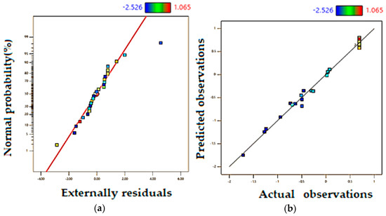
Figure 10. Model performance (a) normal plot of residuals and (b) predicted vs. actual observations for Y_d.

Table 13. ANOVA results of the Y_d in function of X_f, X_s, X_p and X_g.

Source	Sum of Squares	DF	Mean Square	F-Value	p-Value	Contribution (%)
Model	14.54	19	0.7654	41.91	<0.0001	3.81
Xf	1.95	1	1.95	106.56	<0.0001	9.70
Xs	1.27	1	1.27	69.5	<0.0001	6.32
Xp	0.9667	1	0.9667	52.94	0.0002	4.81
Xg	1.57	1	1.57	85.77	<0.0001	7.81
XfXs	1.36	1	1.36	74.29	<0.0001	6.77
XfXp	2.14	1	2.14	117.3	<0.0001	10.65
XfXg	1.11	1	1.11	60.73	0.0001	5.52
XsXp	1.26	1	1.26	68.74	<0.0001	6.27
XsXg	0.6937	1	0.6937	37.98	0.0005	3.45
XpXg	1.26	1	1.26	68.85	<0.0001	6.27
Xf²	1.24	1	1.24	68.16	<0.0001	6.17
Xs²	1.39	1	1.39	76.02	<0.0001	6.91
Xg²	0.0739	1	0.0739	4.04	0.0842	0.37
XfXsXg	0.0719	1	0.0719	3.93	0.0877	0.36
XfXpXg	0.2165	1	0.2165	11.86	0.0108	1.08
Xf²Xs	0.8362	1	0.8362	45.79	0.0003	4.16
Xf²Xp	0.6394	1	0.6394	35.02	0.0006	3.18
XfXg²	1.19	1	1.19	65.29	<0.0001	5.92
XsXg²	0.0986	1	0.0986	5.4	0.0531	0.49
Residual	0.1278	7	0.0183
Cor Total	14.67	26

Regarding the effect of the different terms of the equation on Y_d, the ANOVA results can be used to find the major factors that affect Y_d. The major contributor is the two factors interaction between X_f and X_p which contributes to about 10.65%. The linear effect of X_f is statistically significant. It contributes to about 9.7% of the data variance of the response Y_d. The effect of the X_g is also significant, it comes after X_f with a contribution percentage of 7.81%. The effect of X_s is significant; it contributes to about 6.91%. The interaction effect between X_f and X_s contributes to 6.77%. The linear effect of X_s contributes to 6.32%. Moreover, the interaction effect between X_s and X_p contributes to 6.27%. All of these forms of the effect of X_s contributes to about 26.27% of the data variance of Y_d. The other significant confronters can be represented by X_p X_g, X_f², X_f X_g², X_f X_g, X_p, X_f²X_s, X_s X_g, X_f²X_p, and X_f X_p X_g; all of these factors contribute to about 40.5 of the variation of Y_d. The interaction effect among the four variables is significant at all levels, as shown in Figure 11a for X_f X_p and Figure 11b for X_f X_g with linear and quadratic forms. The three factors interaction is weak and only noticed between X_f X_p X_g with a small contribution of 1.08%.

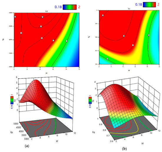
Figure 11. The effect of (a) X_f X_p and (b) X_f X_g on Y_d (2D to 3D).

3.2.2. Modeling of Weld Aspect Ratio (Y_r)

For the output response (Y_r), the cubic polynomial model with square root transformation gives the best fit. The auto-select of terms relying on the adjusted R² were adjusted. The obtained mathematical formulation for Y_r can be represented as Equation (7).

$$\sqrt{Y_r}=-8.2149+1.9443 X_f+4.72 \times {10}^{-3} X_s-5.12 \times {10}^{-3} X_p+21.2945 X_g-2.79 \times {10}^{-4} X_f{X}_s+2.36 \times {10}^{-4} X_f{X}_p-5.1516 X_f{X}_g-3.29 \times {10}^{-7} X_s{X}_p-8.16 \times {10}^{-3} X_s{X}_g+0.0119 X_p{X}_g+6.26 \times {10}^{-4} X_f²-10.2674 X_g²+4.08 \times {10}^{-7} X_s{X}_g+1.90 \times {10}^{-5} X_f²X_s-1.60 \times {10}^{-5} X_f² X_p+3.0623 X_f{X}_g²+3.52 \times {10}^{-3} X_s{X}_g²-7.42 \times {10}^{-3} X_p{X}_g²$$

(7)

In Table 14, the residuals are collected showing the accuracy of the predicted values for the Y_r mathematical models. The residual values for Y_r were very low attesting that the pathway followed in our modeling is conclusive and closer to the actual phenomena occurred in the weld pool within the range of the welding conditions used.

Table 14. Residues calculation for validation of the Y_r mathematical model.

Exp. Number	Xf	Xs	Xp	Xg	Yr	$\mathbf{Transformed} \mathbf{Actual} \mathbf{Value}=\sqrt{{\mathit{Y}}_{\mathit{r}}}.$	Predicted Value	Residual
1	2	1500	3000	1	2.52	1.59	1.56	0.0285
2	2	3000	3000	1	2	1.41	1.41	0.0047
3	2	3000	5000	1	2	1.41	1.4	0.0095
4	2	4500	5000	1	2.31	1.52	1.56	−0.0427
5	12	1500	3000	1	0.2	0.4472	0.4132	0.034
6	12	3000	3000	1	0.18	0.4243	0.4915	−0.0672
7	12	3000	5000	1	0.23	0.4796	0.5771	−0.0976
8	12	4500	5000	1	0.43	0.6557	0.525	0.1307
9	7	1500	3000	1	1.89	1.37	1.42	−0.0465
10	7	3000	3000	1	0.76	0.8718	0.8253	0.0465
	7	3000	5000	1	2.5	1.58	1.53	0.0465
12	7	4500	5000	1	0.58	0.7616	0.8081	−0.0465
13	2	1500	3000	2	2.9	1.7	1.7	−0.0001
14	2	3000	3000	2	2	1.41	1.46	−0.0476
15	2	3000	5000	2	2.4	1.55	1.55	0.0009
16	2	4500	5000	2	2.53	1.59	1.54	0.0468
17	12	1500	3000	2	0.51	0.7141	0.7202	−0.0061
18	12	3000	3000	2	0.18	0.4243	0.3705	0.0537
19	12	3000	5000	2	0.62	0.7874	0.7822	0.0052
20	12	4500	5000	2	0.38	0.6164	0.6693	−0.0529
21	2	1500	3000	3	0.34	0.5831	0.6658	−0.0827
22	2	3000	3000	3	1.7	1.3	1.21	0.0972
23	2	3000	5000	3	0.08	0.2828	0.2645	0.0183
24	2	4500	5000	3	0.27	0.5196	0.5525	−0.0328
25	12	1500	3000	3	0.57	0.755	0.6906	0.0644
26	12	3000	3000	3	1.09	1.04	1.12	−0.0789
27	12	4500	5000	3	0.49	0.7	0.6855	0.0145

The statistical analysis shows a good fitting level of the proposed model to represent the observed/measured data. As shown in Figure 12a, the residuals are normally distributed. The errors are random and normally distributed. It implies that the model captures the main patterns and sources of variation in the data and that the errors are random and independent which indicates the accuracy of the model. Moreover, Figure 12b shows a satisfactory distribution of the actual data against the predicted data. The ANOVA results for Y_r are listed in Table 15. As shown, the F-value = 29.91 is good with a p-value < 0.0001 which indicates that the proposed equation fits the measured data. The obtained R² = 0.9854, the adjusted R² = 0.9524, and the predicted R²= 0.8406; these values confirm the statistical significance of the mathematical model with an acceptable level. Regarding the signal to noise ratio S/N = 16.92 > 4, i.e., that which indicates an adequate signal. These statistical Figures support the statistical significance of the proposed relation to predicting Y_r in the function of the four parameters X_f, X_s, X_p, and X_g and their different interactions and orders.

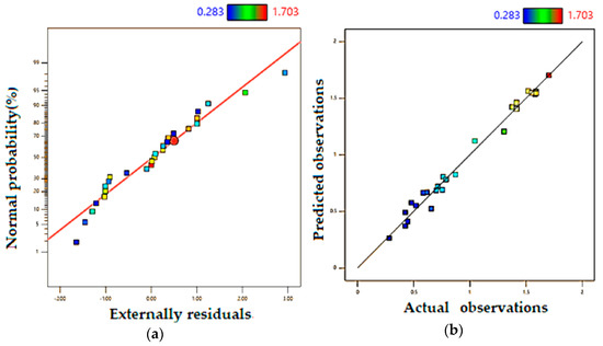
Figure 12. Model statistical indicators (a) Normal Plot of Residuals (b) Predicted vs. Actual observations for Y_r.

Table 15. ANOVA results of the Y_r in function of X_f, X_s, X_p and X_g.

Source	Sum of Squares	DF	Mean Square	F-Value	p-Value	Contribution (%)
Model	5.53	18	0.3072	29.91	<0.0001	4.59
Xf	1.72	1	1.72	167.64	<0.0001	25.73
Xs	0.5878	1	0.5878	57.22	<0.0001	8.79
Xp	0.4856	1	0.4856	47.27	0.0001	7.26
Xg	0.2437	1	0.2437	23.72	0.0012	3.64
Xf Xs	0.0175	1	0.0175	1.71	0.2279	0.26
Xf Xp	0.0565	1	0.0565	5.5	0.047	0.85
Xf Xg	0.8492	1	0.8492	82.67	<0.0001	12.70
Xs Xp	0.0001	1	0.0001	0.0109	0.9193	0.00
Xs Xg	0.2414	1	0.2414	23.5	0.0013	3.61
Xp Xg	0.1785	1	0.1785	17.38	0.0031	2.67
Xf²	0.2701	1	0.2701	26.29	0.0009	4.04
Xg²	0.2763	1	0.2763	26.9	0.0008	4.13
Xs Xp Xg	0.0604	1	0.0604	5.88	0.0415	0.90
Xf² Xs	0.4127	1	0.4127	40.17	0.0002	6.17
Xf²Xp	0.2018	1	0.2018	19.65	0.0022	3.02
Xf Xg²	0.6501	1	0.6501	63.28	<0.0001	9.72
XsXg²	0.0343	1	0.0343	3.34	0.1049	0.51
XpXg²	0.0826	1	0.0826	8.04	0.022	1.24
Residual	0.0822	8	0.0103
Cor Total	5.61	26

Concerning the different terms of the equation, the ANOVA results show the statistical significance of the linear terms and the effect of their interactions. The factor X_f is responsible for the main effect and contributes to about 25.73% of the data variance. The second and third terms are the interaction between X_f and, respectively X_g and the quadratic form of X_g². These two interactions contribute to about 22.4% of the data variance. This interaction relationship between X_f and X_g can be illustrated in Figure 13a. As shown in this figure, the contour lines are of higher orders. In addition, the quadratic form of X_f gives a significant interaction effect with each of X_s and X_p with about 9.19% of the two terms. The interaction of X_f and X_s is shown in Figure 13b. The effects of X_s and X_p on Y_r are significant and their contributions on the data variance of Y_r can be consider as to be similar. Many other terms are statistical significant, that have p-value < 0.05. These terms include X_g², X_f², X_g, X_s X_g, X_f²X_p, X_p X_g, X_pX_g², X_s X_p X_g, and X_f X_p. Their aggregated contribution effect on the variation of Y_r is about 24.1%. The effects of the other terms on Y_r are statistically insignificant where the p-value > 0.05. These terms represent the interaction effect of X_sX_g², X_f X_s, and X_s X_p.

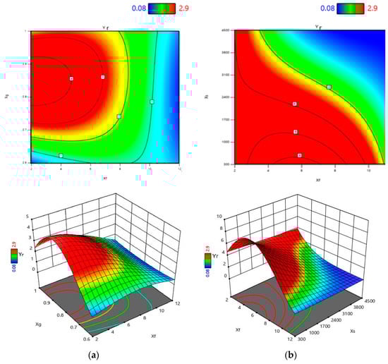
Figure 13. The effect of (a) X_f X_g (b) X_f X_s on Y_r (2D to 3D).

3.2.3. Modeling of Weld Bead Area (Y_a)

The response variable Y_a is modeled as represented in Equation (8) using the cubic polynomial model. The response Y_a was transformed using inverse square transformation. Furthermore, the auto-select of terms relying on the adjusted R² were adjusted.

$$\frac{1}{\sqrt{Y_a}}=1.8122-0.2114 {X_f}_{ }-2.40 \times {10}^{-5} {X_s}_{ }+4.84 \times {10}^{-4} {X_p}_{ }-5.1059 {X_g}_{ }+7.10 \times {10}^{-5} XX-9.00 \times {10}^{-5} X_{f}X+0.7314 X_{f}X+4.48 \times {10}^{-8} X_{s}X-5.82 \times {10}^{-4} X_{s}X-5.29 \times {10}^{-4} X_{p}X-9.21 \times {10}^{-4} X_f²-3.63 \times {10}^{-8} X_s²+3.5446 X_g²-2.40 \times {10}^{-5} X_f{X}_s {X_g}_{ }+3.80 \times {10}^{-5} X{X}_{p}X-3.02 \times {10}^{-6} X_f² {X_s}_{ }+3.18 \times {10}^{-6} X_f² {X_p}_{ }-0.4795 X_f{X}_g²+5.73 \times {10}^{-4} X_s{X}_g²$$

(8)

Table 16 represents the residues calculation for validation of the Y_a mathematical models. The predicted values of Y_a matches accurately the experimental Y_a results.

Table 16. Residues calculation for validation of the Y_a mathematical model.

Run Order	Xf	Xs	Xp	Xg	Ya	$\mathbf{Transformed} \mathbf{Actual} \mathbf{Value}=\frac{1}{\sqrt{{\mathit{Y}}_{\mathit{a}}}}$	Predicted Value	Residual
1	2	1500	3000	1	67	0.1222	0.1416	−0.0195
2	2	3000	3000	1	55.5	0.1342	0.122	0.0122
3	2	3000	5000	1	48	0.1443	0.1478	−0.0035
4	2	4500	5000	1	46.5	0.1466	0.1359	0.0107
5	12	1500	3000	1	12.5	0.2828	0.2822	0.0007
6	12	3000	3000	1	8	0.3536	0.3497	0.0039
7	12	3000	5000	1	17	0.2425	0.2333	0.0092
8	12	4500	5000	1	15	0.2582	0.272	−0.0138
9	7	1500	3000	1	98.5	0.1008	0.1096	−0.0088
10	7	3000	3000	1	24	0.2041	0.1953	0.0088
11	7	3000	5000	1	68.5	0.1208	0.112	0.0088
12	7	4500	5000	1	39	0.1601	0.1689	−0.0088
13	2	1500	3000	2	73	0.117	0.1141	0.0029
14	2	3000	3000	2	47	0.1459	0.147	−0.0011
15	2	3000	5000	2	50	0.1414	0.1425	−0.0011
16	2	4500	5000	2	47	0.1459	0.1466	−0.0007
17	12	1500	3000	2	18.5	0.2325	0.2353	−0.0028
18	12	3000	3000	2	8	0.3536	0.3519	0.0016
19	12	3000	5000	2	28	0.189	0.1887	0.0003
20	12	4500	5000	2	13	0.2774	0.2765	0.0008
21	2	1500	3000	3	11	0.3015	0.2886	0.0129
22	2	3000	3000	3	50	0.1414	0.1489	−0.0075
23	2	3000	5000	3	4	0.5	0.5075	−0.0075
24	2	4500	5000	3	8.6	0.341	0.339	0.002
25	12	1500	3000	3	17.9	0.2364	0.2438	−0.0074
26	12	3000	3000	3	9	0.3333	0.3293	0.004
27	12	4500	5000	3	12	0.2887	0.2853	0.0034

The significance of the proposed model can be noticed via the statistical analysis. Figure 14a shows the normal plot of residuals and the Figure 14b predicted against the actual transformed data. As shown, the plots are well distributed around the reference lines. Scanty residuals, as depicted in Table 16, indicate a good accuracy of the regression model. The ANOVA results confirm the statistical significance of the proposed formulation, as listed in Table 17. The statistical indicators are as follows: F-value = 56.3, R² = 0.9935, the adjusted R² = 0.9759, the predicted R² = 0.8668. The values of the adjusted R² and the predicted R² indicate a reasonable agreement where the difference between them is small (less than 0.2), indicating the statistical significance of the equation. Moreover, the signal-to-noise ratio is sufficiently good, S/N = 30.15 (values > 4 are considered good), which shows the adequacy of the model to represent the data.

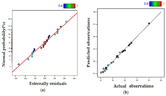
Figure 14. Model performance (a) normal plot of residuals and (b) predicted vs. actual observations of Y_a.

Table 17. ANOVA results of Y_a in function of X_f, X_s, X_p and X_g.

Source	Sum of Squares	DF	Mean Square	F-Value	p-Value	Contribution (%)
Model	0.2515	19	0.0132	56.3	<0.0001	3.61
Xf	0.017	1	0.017	72.23	<0.0001	4.65
Xs	0.0184	1	0.0184	78.19	<0.0001	5.04
Xp	0.0156	1	0.0156	66.42	<0.0001	4.27
Xg	0.0366	1	0.0366	155.46	<0.0001	10.02
Xf Xs	0.0302	1	0.0302	128.26	<0.0001	8.27
Xf Xp	0.0508	1	0.0508	216.23	<0.0001	13.91
Xf Xg	0.0266	1	0.0266	113.25	<0.0001	7.28
Xs Xp	0.0229	1	0.0229	97.43	<0.0001	6.27
Xs Xg	0.0096	1	0.0096	41	0.0004	2.63
Xp Xg	0.0196	1	0.0196	83.56	<0.0001	5.37
Xf²	0.0197	1	0.0197	83.64	<0.0001	5.39
Xs²	0.026	1	0.026	110.37	<0.0001	7.12
Xg²	0.0068	1	0.0068	28.76	0.001	1.86
Xf Xs Xg	0.0049	1	0.0049	20.7	0.0026	1.34
Xf Xp Xg	0.0098	1	0.0098	41.7	0.0003	2.68
Xf² Xs	0.0093	1	0.0093	39.53	0.0004	2.55
Xf²Xp	0.0096	1	0.0096	40.71	0.0004	2.63
Xf Xg²	0.0168	1	0.0168	71.37	<0.0001	4.60
XsXg²	0.0018	1	0.0018	7.8	0.0268	0.49
Residual	0.0016	7	0.0002
Cor Total	0.2532	26

For investigating the significance of the different terms of the equation, the ANOVA results can be used to find the major factors that affect Y_a. As shown in Table 17, all the equation terms are significant at 95% confidence level, i.e., p-value < 0.05. After computing the percentage of contribution of each factor, the effect of X_g (= 10%) is found to be greater than the effects of the other factors X_f (= 4.65%), X_s (= 5%), and X_p (= 4.27%). The aggregated effect of the linear model contributes to about 24%. However, the two factor interaction effect of X_f with the different factors forms the main contributors. These effects can be represented by X_f X_p, X_f X_s, and X_f X_g. The three terms represent a contribution of about 29.5% of the data variance of Y_a. These interaction effects can be represented in Figure 15 for both X_f X_p in Figure 15a, and X_f X_g in Figure 15b. The other two levels interactions are also significant that includes X_s X_p, X_s X_g and X_p X_g. These three terms contribute about 14.27% of the Y_a variation. Moreover, the two factors with linear–quadratic interactions effect are significant. These forms can be represented by X_f X_g² (4.6%), X_f²X_p (2.63%), X_f² X_s (2.55%), and X_sX_g² (0.49%). These four components are responsible of about 10.27% of the variation of Y_a. Accordingly, the two factor interaction is the major factor responsible for the variation of Y_a with a total contribution of 54%. The quadratic terms of the X_f², X_s² and X_f² are also significant and affect Y_a with reasonable percentage: X_s² (= 7.12%), X_f² (= 5.4%) and X_g² (= 1.86%). Regarding the three factor interactions, only X_f X_s X_g and X_f X_p X_g are significant, with an aggregated contribution of about 4%.

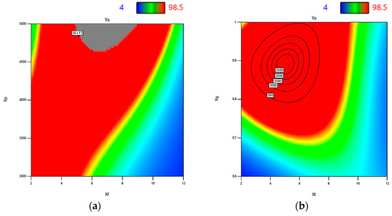
Figure 15. The effect of (a) X_f and X_p and (b) X_f and X_g on Y_a (2 D).

3.3. Surface Surfactant Element and the Laser Weld Morphology

This section is dedicated to analyze the role of surfactant elements, such as sulfur, in determining the laser weld shape within the used laser welding parameters. In high sulfur content cast (316 HS), the depth of weld is greater than that of low sulfur content, however, the width of latter cast is greater than of 316 HS cast. In 316 HS weld pool, the molten metal moves in inward circulation leading to deeper and narrower weld (reverse Marangoni convection). In 316 LS weld pool, the molten metal moves in outward circulation leading to wider and shallower weld bead [27,28,29]. Our study answered the following question: is the role of surfactant elements important in determining the shape of the laser weld? Table 18 represents the results of the 27 tests carried out for both casts.

Table 18. Depth penetration and width weld bead measurements for 316 HS and LS casts.

Exp. Number	Cast 316 HS			Cast 316 LS			Occurrence of Inverse Marangoni Convection for 316 HS Cast and Occurrence of Conventional Marangoni Convection for 316 LS Cast
	Inverse Marangoni Convection			Marangoni Convection
	Weld Depth (D) (mm)	Weld Width (W) (mm)	Full Penetration Weld (F.P)/ Partial Penetration Weld (P.P)	Weld Depth (D) (mm)	Weld Width (W) (mm)	Full Penetration Weld (F.P)/ Partial Penetration Weld (P.P)
1	2	0.58	F.P	2	0.79	F.P	Yes
2	2	1.15	F.P	2	1	F.P	No
3	2	1.40	F.P	2	1	F.P	No
4	2	1.22	F.P	2	0.86	F.P	No
5	0.6	1.43	P.P	0.39	1.95	P.P	Yes
6	0.35	0.27	P.P	0.29	1.61	P.P	Yes
7	0.62	0.84	P.P	0.48	2.1	P.P	Yes
8	0.44	1.33	P.P	0.61	1.42	P.P	No
9	2	1.27	F.P	2	1.06	F.P	No
10	1.15	1.17	P.P	0.93	1.22	P.P	Yes
11	2	0.69	F.P	2	0.8	F.P	Yes
12	1.09	0.65	P.P	1.08	1.86	P.P	Yes
13	2	1.68	F.P	2	0.69	F.P	No
14	2	0.82	F.P	2	1	F.P	Yes
15	2	0.89	F.P	2	2.4	F.P	Yes
16	2	0.70	F.P	2	0.83	F.P	Yes
17	0.44	1.76	P.P	0.74	1.45	P.P	No
18	0.38	1.46	P.P	0.28	1.55	P.P	Yes
19	1.12	1.6	P.P	1.04	1.67	P.P	Yes
20	0.72	1.38	P.P	0.53	1.39	P.P	Yes
21	1.98	0.59	P.P	0.63	1.85	P.P	Yes
22	0.65	0.33	P.P	1.8	1.71	P.P	No
23	0.49	1.96	P.P	0.18	2.25	P.P	Yes
24	0.91	0.39	P.P	0.61	2.26	P.P	Yes
25	0.8	1.12	P.P	0.77	1.35	P.P	Yes
26	0.48	1.17	P.P	0.5	0.46	P.P	No
27	0.44	0.44	P.P	0.6	1.22	P.P	No

Among the 27 tests for each cast with a total of 54 welds, the welds were fully penetrated 20 times against 34 times where the chosen welding parameters led to partially penetrated welds, as depicted in Table 18. For each experiment, we compared the behavior of two casts. The inverse Marangoni convection is expected to occur in the 316 HS weld pool, but the conventional Marangoni convection is supposed to happen in the 316 LS weld pool [28]. We notice that the partially penetrated welds are obtained 17 times for both casts, wherein the inverse Marangoni convection occurs 12 times in the 316 HS cast and a conventional Marangoni occurs 5 times in the 316 LS cast; the latter convection modes phenomena especially occurred in 316 HS. Indeed, in partially penetrated welds, 71% welds confirm the occurrence of inverse Marangoni convection in the rich sulfur cast (316 HS) and the occurrence of conventional Marangoni convection in the 316 LS cast. On the other hand, 29 % of welds confirm that the latter convection modes phenomenon does not occur especially for 316 HS, as shown in Table 19.

Table 19. Percentages of occurrences of inverse Marangoni convection for 316 HS and conventional Marangoni convection for 316 LS in laser welds.

Types of Weld Bead	Times Getting Partial Penetration Weld(PP) or Full Penetration Weld (FP) Weld Bead for Both Casts Out of 27 Tests	Occurrence of Inverse Marangoni Convection for 316 HS Cast and Occurrence of Conventional Marangoni Convection for 316 LS Cast For the Same Welding Parameters	Non Predominance of Conventional Marangoni Convection for 316 LS and/or Non Predominance of Inverse Marangoni Convection for 316 HS	Percentages Occurrences of Inverse Marangoni and Conventional Marangoni Convection %
Partial Penetration weld(PP)	17	12	5	71
Full Penetration weld(FP)	10	5	5	50

Fully penetrated welds are achieved 10 times for both casts. The inverse Marangoni convection is confirmed no more than 5 times in the 316 HS cast and the conventional Marangoni convection occurs 50% of the times in the 316 LS cast, as depicted in Table 19. In 50% of welds, the latter convection modes phenomenon does not happen, as shown in Table 19. This is probably related to the fact that the inverse Marangoni convection in the case of a fully penetrated weld is hidden or completely non-existent owing to the aerodynamic behavior of the shield gas at a certain level of energy provided to the workpiece.

4. Conclusions

The aim of this study is to analyze the effects of the basic parameters of laser welding, such as laser beam power, welding speed, type of shield gas as well as energy input in relation with sulfur surface tension agent on the weld shape of 2.0 mm thick stainless steel industrial 316 sheets. This experimental research work was conducted to better understand the role of sulfur on the laser weld shape of 316 SS casts. RSM has been used efficiently to mathematically model the depth and the aspect ratio as well as the weld cross section area as functions of the above cited inputs. Linear and quadratic polynomial models for predicting the weld bead geometry were developed. The following main findings can be drawn:

-

The developed regression equations from the response surface methodology has been used successfully to model geometries of the laser welds of thin plates of 316 stainless steel. The predicted values of geometric weld morphology were close to the actual experimental results.

-

For cast 316 HS, the main input factors influencing the depth weld (Y_d) is the focal point with contribution up to 19.32%. The aspect ratio (Y_r) is influenced by the focal point with a proportion of 70.6% of the data variance. For the weld bead area (Y_a), the major contributor is the interaction of the two factors X_f and X_p. This interaction effect contributes to about 24.25% of the data variance.

-

Regarding cast 316 LS, the main input factors affecting the depth weld (Y_d) is the combination effect of focus point and power input energy with contribution up to 10.65%. The shield gas X_g has a highest contribution up to 25.75% influencing the aspect ratio (Y_r). The combination effect of shield gas X_g and power X_p affect the size area of weld bead (Y_a) up to 13.91%.

-

The role of the shield gas in protecting the weld pool is related to the level of energy supplied. Thus, at high energy level, either helium or mixture gas (70% He + 30% Ar) produces weld beads larger than those produced under the shield gas mixture (40% He + 60% Ar). This is ascribed to the fact that helium is characterized by a high ionization potential, which performs a better protection of the weld pool by expelling the plasma ensuring less loss heat transfer.

-

The surface-active elements fully play their role only in the case where the chosen welding parameters would result in partially penetrated weld. To quantify these results, the statistical study shows that 71% of the partially penetrated weld confirms the role of the surface-active elements of sulfur for the 316 HS cast. However, in the case of fully penetrated welds, the contribution of surfactant elements in determining the shape of the weld bead for the 316 HS cast is diminished or completely hidden. The aerodynamic currents of the shield gas is the more important factor when the level of energy is high, resulting in fully penetrated welds, such that only 50% welds where sulfur as surfactant contributes significantly in imposing the inverse Marangoni convection.

References

- Biswas, A.R.; Banerjee, N.; Sen, A.; Maity, S.R. Applications of laser beam welding in automotive sector—A Review. In Advances in Additive Manufacturing and Metal Joining; Springer: Berlin/Heidelberg, Germany, 2023; pp. 43–57. [Google Scholar]
- Chen, Y.; Sun, S.; Zhang, T.; Zhou, X.; Li, S. Effects of post-weld heat treatment on the microstructure and mechanical properties of laser-welded NiTi/304SS joint with Ni filler. Mater. Sci. Eng. A 2020, 771, 138545. [Google Scholar] [CrossRef]
- Ahmed, A.; Ali, P.; Rasoul, S.; Davood, R. Comparison between laser beam and gas tungsten arc tailored welded blanks via deep drawing. Proc. Inst. Mech. Eng. Part B J. Eng. Manuf. 2020, 235, 673–688. [Google Scholar]
- Esfahani, R.; Coupland, J.; Marimuthu, S. Microstructure and mechanical properties of a laser welded low carbon-stainless steel joint. J. Mater. Process. Technol. 2014, 214, 2941–2948. [Google Scholar] [CrossRef]
- Srinivas, B.; Murali Krishna, N.; Cheepu, M.; Sivaprasad, K.; Muthupandi, V. Studies on post weld heat treatment of dissimilar aluminum alloys by laser beam welding technique. IOP Conf. Ser. Mater. Sci. Eng. 2018, 330, 012079. [Google Scholar] [CrossRef]
- Srinivas, B.; Cheepu, M.; Sivaprasad, K.; Muthupandi, V. Effect of gaussian beam on microstructural and mechanical properties of dissimilar laser welding of AA5083 and AA6061 alloys. IOP Conf. Ser. Mater. Sci. Eng. 2018, 330, 012066. [Google Scholar] [CrossRef]
- Behzad, F.; Steven, F.W.; Gladius, L.; Ebrahim, A. A Review on Melt-Pool Characteristics in Laser Welding of Metals. Adv. Mater. Sci. Eng. 2018, 2018, 4920718. [Google Scholar]
- Ayoola, W.A.; Suder, W.J.; Williams, S.W. Parameters controlling weld bead profile in conduction laser welding. J. Mater. Process. Tech. 2017, 249, 522–530. [Google Scholar] [CrossRef]
- Suder, W.J.; Williams, S. Investigation of the effects of basic laser material interaction parameters in laser welding. J. Laser Appl. 2012, 24, 032009. [Google Scholar] [CrossRef]
- Giudice, F.; Missori, S.; Sili, A. Parameterized Multipoint-Line Analytical Modeling of a Mobile Heat Source for Thermal Field Prediction in Laser Beam Welding. Int. J. Adv. Manuf. Technol. 2021, 112, 1339–1358. [Google Scholar] [CrossRef]
- Pang, S.; Chen, L.; Zhou, J.; Yin, Y.; Chen, T.A. three-dimensional sharp interface model for self-consistent keyhole and weld pool dynamics in deep penetration laser welding. J. Phys. D Appl. Phys. 2011, 44, 025301. [Google Scholar] [CrossRef]
- Zhao, C.; Kwakernaak, C.; Pan, Y.; Richardson, I.M.; Saldi, Z.; Kenjeres, S.; Kleijn, C.R. The effect of oxygen on transitional Marangoni flow in laser spot welding. Acta Mater. 2010, 58, 6345–6357. [Google Scholar] [CrossRef]
- Chan, C.; Mazumder, J.; Chen, M.M. A two-dimensional transient model for convection in laser melted pool. Metall. Trans. A 1984, 15, 2175–2184. [Google Scholar] [CrossRef]
- Tomasz, K. Heat Source Models in Numerical Simulations of Laser Welding. Materials 2020, 13, 2653. [Google Scholar]
- Giudice, F.; Sili, A. Weld Metal Microstructure Prediction in Laser Beam Welding of Austenitic Stainless Steel. Appl. Sci. 2021, 11, 1463. [Google Scholar] [CrossRef]
- Möbus, M.; Woizeschke, P. Laser beam welding setup for the coaxial combination of two laser beams to vary the intensity distribution. Weld World 2022, 66, 471–480. [Google Scholar] [CrossRef]
- Quanhong, L.; Manlelan, L.; Zhongyan, M.; An, G.H.; Shengyong, P. Improving laser welding via decreasing central beam density with a hollow beam. J. Manuf. Process 2022, 73, 939–947. [Google Scholar]
- Yongki, L.; Byung-Kwon, M.; Cheolhee, K. Optimization of gas shielding for the vacuum laser beam welding of Ti-6Al-4 titanium alloy. Int. J. Adv. Manuf. Technol. 2022, 123, 1297–1305. [Google Scholar]
- Reuven, K.; Anton, Z.; Amnon, S. Effect of Laser Welding Parameters on Weld Bead Geometry. Res. J. Appl. Sci. Eng. Technol. 2018, 15, 118–123. [Google Scholar]
- Anawa, E.; Olabi, A.-G. Using Taguchi method to optimize welding pool of dissimilar laser-welded components. Opt. Laser Technol. 2008, 40, 379–388. [Google Scholar] [CrossRef]
- Olabi, A.G.; Casalino, G.; Benyounis, K.Y.; Hashmi, M.S.J. An ANN and Taguchi algorithms integrated approach to the optimization of CO2 laser welding. Adv. Eng. Softw. 2006, 37, 643–648. [Google Scholar] [CrossRef]
- Benyounis, K.Y.; Olabi, A.G.; Hashmi, M.S.J. Effect of laser welding parameters on the heat input and weld-bead profile. J. Mater. Process. Technol. 2005, 164–165, 978–985. [Google Scholar] [CrossRef]
- Hasanzadeh, R.; Mogaver, M.; Azdast, T.; Park, C.P. A novel systematic multi-objective optimization to achieve high-efficiency and low-emission waste polymeric foam gasification using response surface methodology and TOPSIS method. Chem. Eng. J. 2022, 430, 1329. [Google Scholar] [CrossRef]
- Mojaver, P.; Khalilarya, S.; Chitsaz, A. Multi-objective optimization using response surface methodology and exergy analysis of a novel integrated biomass gasification, solid oxide fuel cell and high-temperature sodium heat pipe system. Appl. Therm. Eng. 2019, 156, 627–639. [Google Scholar] [CrossRef]
- Ma, Z.; Dan, H.; Tan, J.; Li, M.; Li, S. Optimization Design of MK-GGBS Based Geopolymer Repairing Mortar Based on Response Surface Methodology. Materials 2023, 16, 1889. [Google Scholar] [CrossRef]
- Shahab, A. Contribution a L’etude de la Metallurgie du Soudage de L’inconel 625 et des Aciers Inoxydables 304 et 316. Ph.D. Thesis, University of Nantes, Nantes Cedex, France, 1990. [Google Scholar]
- Heiple, C.R.; Roper, J.R.; Stagner, R.T.; Aden, R.J. Surface Active Element Effects on the Shape of GTA, Laser, and Electron Beam Welds. Weld. Res. Suppl. 1983, 62, 72–77. [Google Scholar]
- Vlastimil, N.; Lenka, R.C.; Petra, V.N.; Michal, S.; Dalibor, M.; Katerina, K.; Bedrich, S.; Silvie, R.; Markéta, T.; L’ubomíra, D.; et al. The Effect of Trace Oxygen Addition on the Interface Behavior of Low-Alloy Steel. Materials 2022, 15, 1592. [Google Scholar]
- Kamel, T.; Abdeljlil, C.H.; Rachid, D.; Abousoufiane, O.; Abdallah, B.; Albaijan, I.; Hany, S.A.; Mohamed, M.Z.A. Mechanical, Microstructure, and Corrosion Characterization of Dissimilar Austenitic 316L and Duplex 2205 Stainless-Steel. ATIG Welded Jt. Mater. 2022, 15, 2470. [Google Scholar]
Disclaimer/Publisher’s Note: The statements, opinions and data contained in all publications are solely those of the individual author(s) and contributor(s) and not of MDPI and/or the editor(s). MDPI and/or the editor(s) disclaim responsibility for any injury to people or property resulting from any ideas, methods, instructions or products referred to in the content. |
© 2023 by the authors. Licensee MDPI, Basel, Switzerland. This article is an open access article distributed under the terms and conditions of the Creative Commons Attribution (CC BY) license (https://creativecommons.org/licenses/by/4.0/).