Article

Damage Distribution Map Based Damage Accumulation Calculation Approach for Welded Joints

1
Key Laboratory of Metallurgical Equipment and Control Technology, Ministry of Education, Wuhan University of Science and Technology, Wuhan 430081, China
2
Hubei Key Laboratory of Mechanical Transmission and Manufacturing Engineering, Wuhan University of Science and Technology, Wuhan 430081, China
3
Precision Manufacturing Institute, Wuhan University of Science and Technology, Wuhan 430081, China
*
Author to whom correspondence should be addressed.
Metals 2023, 13(7), 1203; https://doi.org/10.3390/met13071203
Submission received: 5 June 2023 / Revised: 24 June 2023 / Accepted: 26 June 2023 / Published: 28 June 2023

Abstract

:
Fatigue damage accumulation under variable amplitude loadings is vital for the life prediction of welded structures. An approach based on damage distribution mapping is presented. S-N curves of welded joints are utilized to construct fatigue damage zones, and a corresponding polynomial fitting function is derived from the heat transfer FEA solution. Experimental results for cruciform and T joints under tensile and three-point bending are employed for validation. Compared with four existing damage models, the proposed approach shows greater accuracy and provides a better description for the early stage of fatigue.

1. Introduction

Fatigue is the local damage accumulating process caused by cyclic loadings on or near the surfaces of materials and structures [1]. After bearing a certain number of cycles, cracks or fracture occur in the damaged areas, thereby causing loss of structural integrity and leading to functional failure. From a certain point of view, the fatigue process is indeed a damage evolution process. Thus, how to describe damage accumulation behavior and evolution processes is vital for fatigue analysis and life prediction [2,3].
In 1945, Miner proposed a linear damage accumulation rule for the first time, according to which fatigue damage was defined as the ratio of loading cycles to the fatigue life corresponding to the stress levels [4]. Miner’s rule assumes that the damage caused by different stress levels can be simply superimposed and is in essence a linear model. Therefore, it is easy to use and recommended by almost all fatigue design standards and codes, such as IIW, BS7608, Euro code, DNVGL, etc. However, some experiments have shown that Miner’s rule is prone to overestimating the fatigue life of “H-L” load spectrums and underestimates the fatigue life of “L-H” load spectrums due to ignorance of the load sequence effect [5,6]. In 1954, Macro and Starkey adopted the damage curve concept and proposed the nonlinear damage theory [7]. Generally, the nonlinear damage theory should be more accurate due to the description of real fatigue damage evolution, whereas appropriate nonlinear damage models are difficult to obtain. Manson and Halford refined the damage curve by linearization and proposed a double linear damage rule (DLDR) [8], according to which two damage lines were utilized to describe the crack initiation and propagation stages, respectively. To some extent, the DLDR or improved DLDR maintains both the simplicity of Miner’s rule and some physical basis, greatly improving the accuracy of life prediction [9,10,11]. Moreover, Miller and Zachariah developed the double exponential law based on the idea of the DLDR [12]. Later, Manson pointed out that the knee point of the DLDR model may not directly relate to the fatigue stage division; therefore, its physical basis is questionable.
Some researchers have attempted to construct nonlinear damage curves in different ways. Chaboche proposed the damage curve description (DCD) method [13,14], in which the fatigue damage caused by a loading cycle could be mathematically described by continuous damage mechanics. Based on the DCD method, similar models have been proposed [15,16,17]. In 1976, Subramanyan noted isodamage lines corresponding to certain stress levels and thought that they were another form of damage curves [18]. Considering that S-N curves describe the loading counts corresponding to failure under different stress levels, they are indeed isodamage curves with fatigue damage of 1. Based on this idea, some researchers have assumed that all the isodamage lines corresponding to different stress levels converge at the knee point of the S-N curve, and they developed damage accumulation models. This hypothesis has been verified by some measured data regarding surface hardness evolution in the fatigue damage accumulation process and has been gradually accepted in recent years [19,20,21]. Meanwhile, a variety of similar models have been proposed, such as the Aeran model [22], the Rege model [23], the Zhu model [24], etc. These models only require S-N curves of the materials and a few other parameters, resulting in good engineering operability. On the other hand, Hashin and Rotem assumed that the isodamage lines should converge at the point where the S-N curve intersects the S-axis, and they proposed an alternative damage accumulation model [25]. Moreover, Pavlou integrated the ideas of Subramanyan, Hashin and Rotem and believed that the isodamage curve should converge both at the knee point of the S-N curve and at the intersecting point of the S-N curve and the S-axis [26]. With the aid of FEA, he proposed a new theory based on the “S-N fatigue damage envelope” for the estimation of fatigue damage accumulation and the prediction of the remaining crack initiation life under variable loadings.
It was advantageous for Pavlou’s theory that no extra damage material parameters were required except S-N curves, leading to great convenience for application to welded structures due to the abundant S-N curves provided in related standards and codes for a variety of welded joint categories. However, the S-N curves in such standards and codes are usually only practicable in a specific life range (104–107 cycles), causing them not to be directly utilized according to Pavlou’s approach. Additionally, several S-N curves with different survival probabilities are usually provided for certain welded joints in those standards and codes. Therefore, how to determine the appropriate S-N curve and construct a reasonable fatigue damage envelope becomes vital and should be more deeply investigated.
In this paper, based on the Pavlou’s theory, a nonlinear damage accumulation approach for welded structures is presented. Using an FEA-based solution for a heat transfer problem, the damage distribution map and the corresponding function for welded joints are derived, and further, the cumulative damage calculation and the fatigue life prediction are realized. Tensile and three-point-bending fatigue tests for cruciform joints and T joints under two-level loading block sequences are conducted. Five models, including Miner, DLDR, Aeran, Rege, and the proposed approach, are utilized for validation, among which the proposed approach shows greater accuracy. Most importantly, compared with the four other models, the proposed approach is able to reasonably describe the early damage characteristics of weld toe cracks.

2. The Proposed Approach and Its Calculation Process

2.1. Damage Distribution Map (DDM)

The basic idea of a DDM can be derived from the concept of isodamage lines, as shown in Figure 1. In Figure 1a, the solid line is the S-N curve for a material in log–log coordinates. Thus, the vertical axis corresponds to the stress range ΔS, and the horizontal axis corresponds to the fatigue life N. From the physical view, the S-N curve can describe the critical damage states under different stress levels, in which only fatigue failures occur, and all the damage values equal 1. Therefore, the S-N curve is in fact an isodamage line with D = 1. Some researchers believe that lines down the S-N curve can represent other isodamage lines, such as the dashed lines converging to the knee point of the S-N curve in Figure 1a, corresponding to decreasing damage values D = 0.75, 0.5, 0.25, etc. Assuming that there is a horizontal line corresponding to a certain stress range intersecting with all the isodamage lines, the abscissa of the intersecting point with the solid line (D = 1) represents the fatigue life under the corresponding stress range, while those intersecting points with dashed lines represent the loading cycles required to reach corresponding damage values. Keeping the horizontal coordinate unchanged and taking damage D as the vertical coordinate, points on the same horizontal line (that is, with the same stress range) can be transformed into a curve, which is in fact the isostress curve, as shown in Figure 1b. Figure 1c also shows some isostress curves with horizontal coordinates that are normalized. It can be seen that isostress curves can clearly describe the tendency of the damage evolution under a certain stress range.
By further investigating the isodamage curves in Figure 1a, it can be seen that the dashed isodamage line at the bottom corresponds to the fatigue limit Se of the material with D = 0, which is reasonable since stress ranges less than the fatigue limit will not lead to any fatigue damage. Referring to the points on the S-axis, based on the isodamage line definition in Figure 1a, their damage is non-zero and decreases from 1 to 0 along the S-axis downward, which is somewhat inconsistent with the actual mechanical behaviors. According to the experimental observations, although the material bears larger loads approaching the yield strength, it will experience at least hundreds or even thousands of cycles due to local strengthening. Indeed, considering that the abscissa of the points on the S-axis are all 0, it seems more reasonable to define their damage values as 0 since those points correspond to 0 cycles, indicating that they are under the initial states with no damage caused. For this reason, Pavlou regarded the S axis as an isodamage line with D = 0 as well and suggested that both the N-axis (the fatigue limit line) and the S-axis should simultaneously move toward the S-N curve with the damage varying from 0 to 1 as the form of curves, as shown in Figure 1d. When the number of these isodamage curves are infinite, the isodamage distribution map will be generated, as shown in Figure 1e,f.

2.2. Construction and Preprocessing of DDM

According to Pavlou’s theory [26], construction of a DDM can be realized by a simple heat transfer problem. Generally, the two-dimensional heat transfer problem can be described as a parabolic partial differential equation, as shown in Equation (1).
T t = k ρ C 2 T x 2 + 2 T y 2
where T is the function of temperature; t is the time; x,y are position coordinates; k is the thermal conductivity; ρ is the density; and C is the specific heat. Considering that the temperature field is steady and constant and assuming a = k ρ C , Equation (1) can be transformed into a Laplace equation, as shown in Equation (2).
2 T = a 2 T x 2 + 2 T y 2 = 0
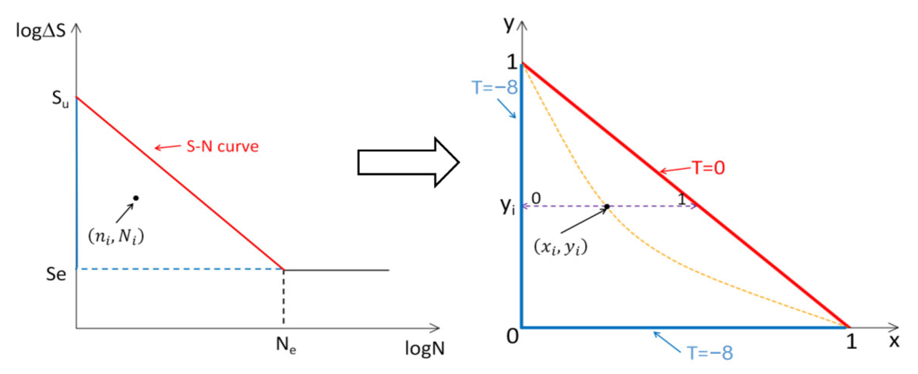
Assuming that the boundary of the heat transfer problem is composed of the S-N curve, S-axis, and N-axis (specifically corresponding to Se), the heat transfer problem can be modeled as shown in Figure 2, in which the x and y coordinates are normalized and can be expressed as Equations (3) and (4), respectively.
x i = n i N i
y i = S i S e S u S e
It can be seen that the bounded area is indeed the damage zone, and points inside it are all damage points with respective damage values, the x coordinates of which denote the ratio of cycles to fatigue life, while the y coordinates denote the relative load ratios. Both the x and y coordinates range between 0 and 1, rendering the heat transfer analysis model simpler and more applicable. It should be emphasized that the x coordinate in Figure 2 should be re-scaled with the damage points moving in the damage zone. Specifically, the abscissa of the intersecting point of the horizontal line through the damage point and the S-N curve is always 1, consistent with the damage connotation of the S-N curve. Based on this outcome, all the abscissas of points on the same horizontal line should be scaled respectively.
According to the literature [26], the boundary condition of the S-N curve can be set as temperature T = logD = 0 since the damage of the S-N curve is D = 1. Referring to the N-axis and S-axis, for the convenience of calculation, a very small value D = 10−8 was used; thus, their boundary conditions can be set as T = logD = log10−8 = −8. All the boundary conditions of the heat transfer problem can be expressed as follows.
b s . S     N   :   T   =   0 b s . S     A x i s   :   T   =   8 b s . N     A x i s   :   T   =   8
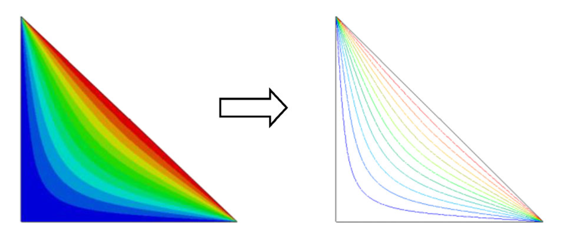
Generally, it is difficult to theoretically solve the heat transfer problem governed by Equations (2) and (5). Numerical methods, such as the FEA method, are usually utilized. Here, a basic FEA code based on Python is used, and the temperature field is obtained, in which a medium-sized mesh model with almost 500 triangular elements is established. According to D = 10T, the damage distribution map is generated, from which isodamage curves can be extracted, as shown in Figure 3.
Since only the damage values of the mesh nodes can be precisely extracted from the DDM due to FEA principles, the damage values of other points in the DDM need to be interpolated. For the convenience of the damage transfer, the damage distribution interpolation function D(x,y) is used here, where D denotes damage, x denotes ni/Ni, and y denotes relative stress Si. By trying a variety of interpolation algorithms, the smoothing spline method-based algorithm exhibits the most satisfying accuracy. Taking the problem in Figure 2 as an example, the sum of squares of fitting errors SSE = 2.778 × 10⁻¹⁷, the square of correlation coefficient R-Square = 0.9935, and the mean square error RMSE = 0.0320. Figure 4 shows the comparison of the DDM between the FEA and interpolation results.
The above construction approach has some advantages: (1) only a few easily available material parameters are required, such as the S-N curve, ultimate strength Su, fatigue limit Se, etc.; (2) theoretically, an infinite number of isodamage curves can be extracted from the continuous DDM; (3) one DDM and the corresponding interpolation function are appropriate for a variety of damage calculation problems with the same boundary configurations. For example, if the S-N curves are a single line, the DDM, as in Figure 3, can be almost directly utilized except for minor treatments. This fact is significant for welded structures because there are many similar S-N curves provided by fatigue design standards and codes according to welded joint classifications. Section 2.2 focuses on such treatments in detail.

2.3. Damage Accumulation Calculation Process

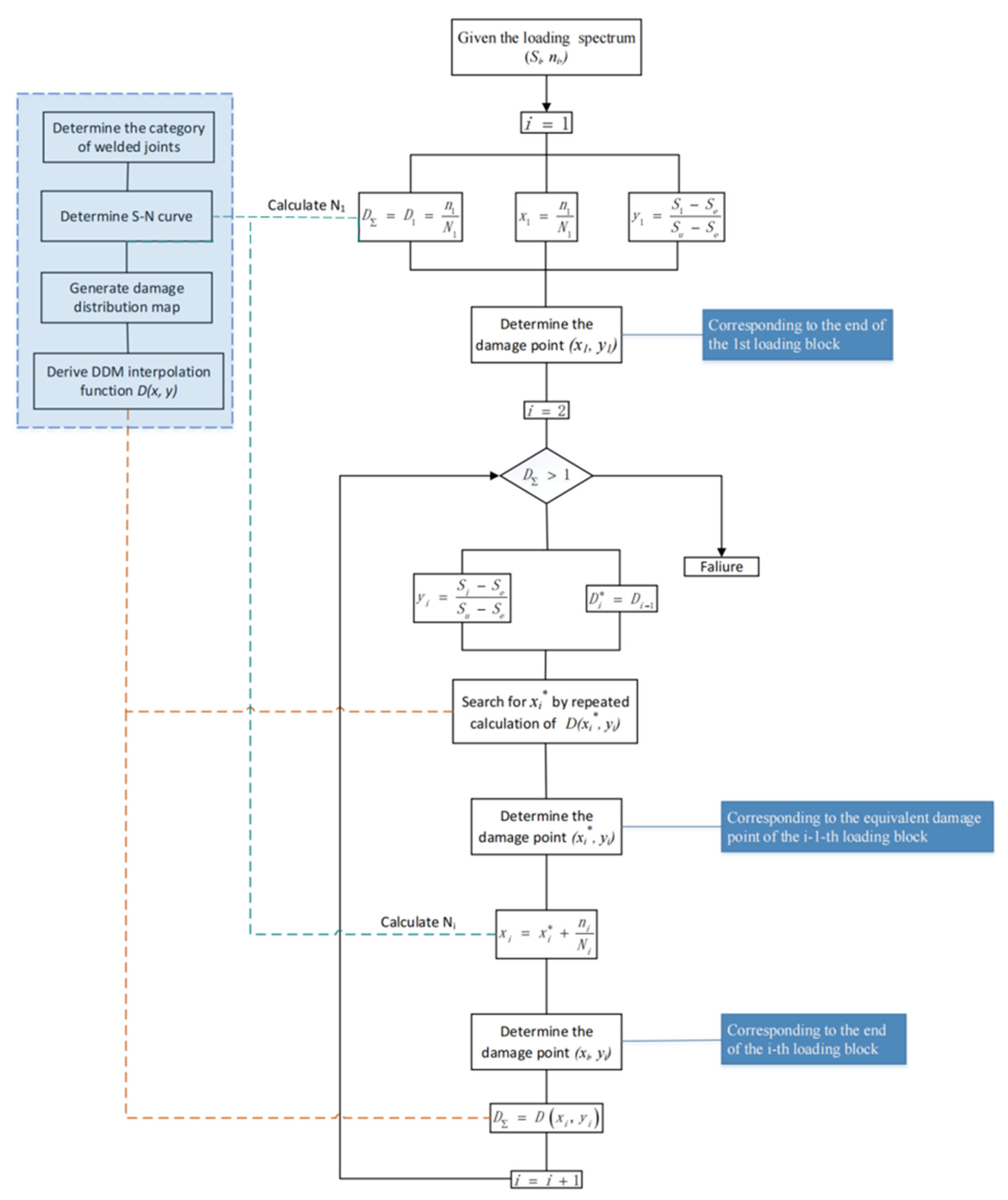
The calculation process of the DDM-based approach is illustrated in Figure 5.
(1) First, the S-N curve should be determined according to the materials or welded joints, which are used to calculate the fatigue life Ni under the i-th constant amplitude loading block. More importantly, the S-N curve will be utilized to construct the DDM by the FEA method, as well as the corresponding interpolation function D(x,y). As mentioned above, the DDM and the function D(x,y) have much better applicability. Once they are generated for some S-N curves with similar shapes, this step need not to be performed again.
(2) Second, damage D1 at the end of the first loading block (S1,n1) should be calculated, and its damage point (x1,y1) in the DDM should be determined. Since this is the first time that the damage is calculated, damage transfer does not happen. Here, the damage D1 = n1/N1, and x1, y1 can be calculated according to Equations (3) and (4).
(3) Third, from the second loading block on, the damage transfer must be introduced. Since there is no explicit description of the isodamage curve in the DDM, the damage distribution interpolation function D(x,y) should be used to search for the appropriate isodamage curve. Specifically, assuming that the damage point at the end of the i−1-th loading block is (xi−1,yi−1), and the damage is Di−1, the damage at the beginning of the i-th loading block can be determined as Di* = Di−1. Then, yi, corresponding to the i-th loading block, can be calculated by Equation (4). Letting xi vary in (0,1) with a small interval, damage calculation trials are conducted based on Equation (3) repeatedly until the calculated damage value approaches Di* in a pre-set tolerance; then, xi* equals to xi. Thus, the transferred damage point (xi*,yi) can be determined. It should be noted that, although the damage points (xi*,yi) are not determined by graphically moving damage points (xi−1,yi−1) along the isodamage curve in the DDM, they do lie on the same isodamage curve.
(4) By adding the damage of only the i-th loading block ni/Ni and the equivalent damage of all the previous loading blocks xi*, the total damage at the end of the i-th loading block xi can be obtained. Then, the damage point (xi,yi) at the end of the i-th loading block can be determined. Finally, the cumulative damage DΣ can be solved by D(xi,yi).
The above steps (3) and (4) are performed repeatedly until the cumulative damage satisfies the failure criterion DΣ > 1.

3. Fatigue Tests of Welded Joints

3.1. Fatigue Test Configuration

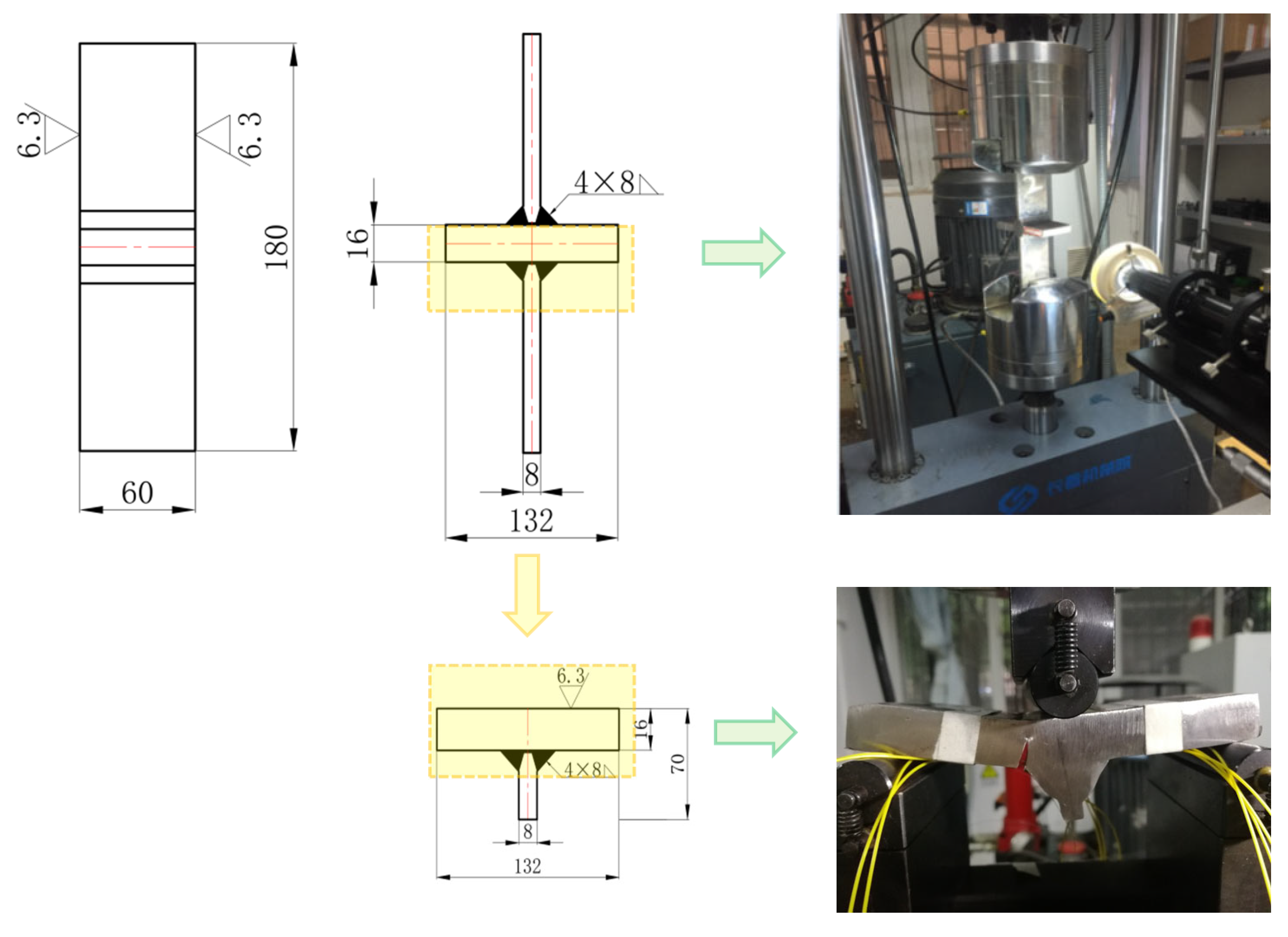
To verify the proposed damage accumulations approach, fatigue tests of cruciform joint specimens and T joint specimens were conducted, as shown in Figure 6. All specimens were first welded and fabricated as cruciform joints with prefabricated grooves based on welding standards to ensure all the welds’ full penetration. The material of the base plates was low alloy structural steel Q345B, and the welding wire used was CHW-50C6. Then, some cruciform joints were cut and fabricated to be T joints, which could keep all the welds of two kinds of specimens with similar welding quality and geometries. The mechanical properties and chemical compositions of Q345B are presented in Table 1 and Table 2, respectively (reported in the specification from the steelmaking plant). The main welding process parameters are reported in Table 3. It should be noted that Q345B has good weldability, leading to a similar yield strength for the base metal and the weld seam. Thus, the strength matching characteristics was not considered in this paper. Moreover, there are also significant differences in the microstructures of different zones, such as the base material, weld seam, and HAZ. However, those differences mainly affect the early stage behaviors, such as crack nucleation and short crack propagation, which are beyond the scope of this paper.
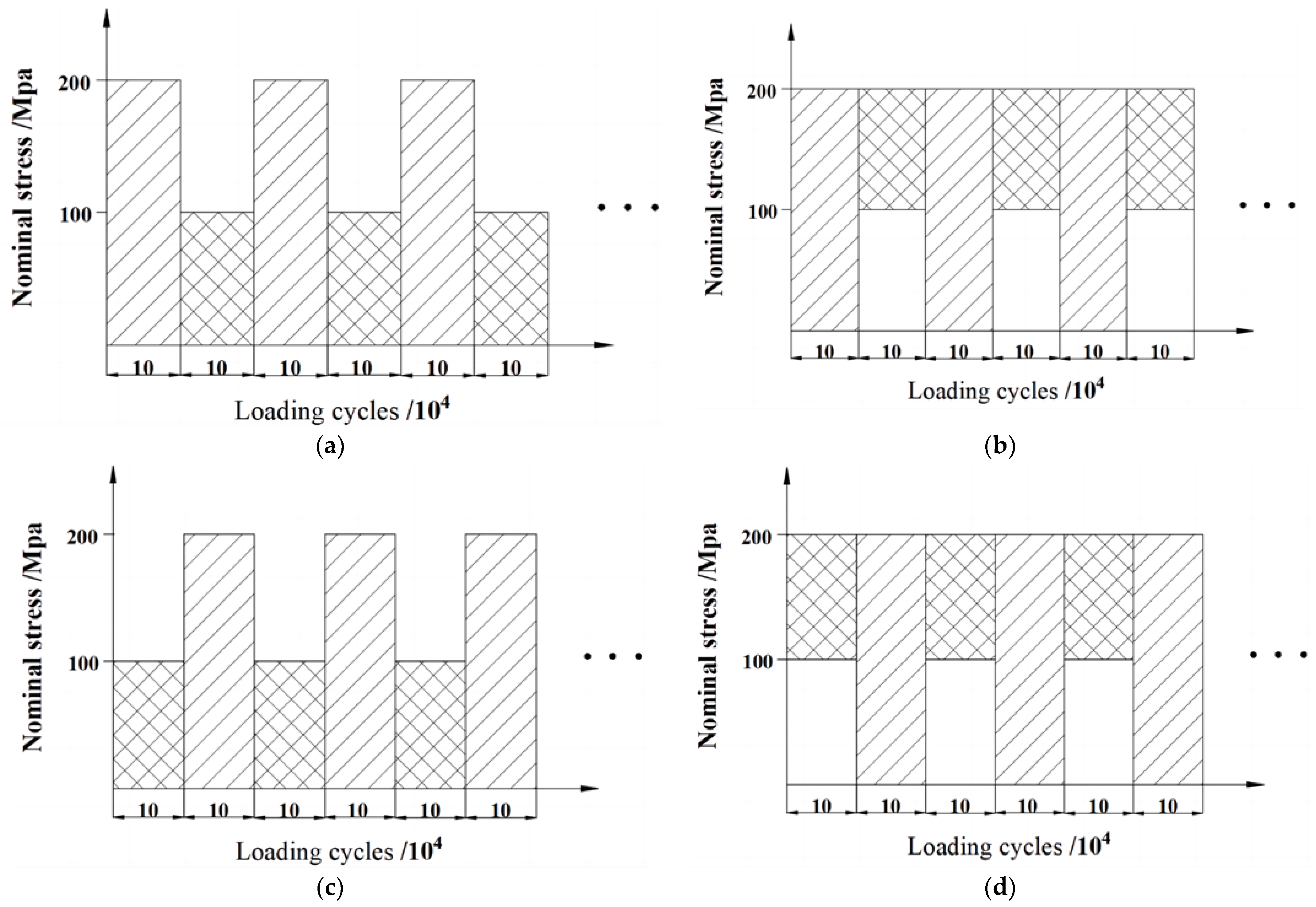
In our research, tensile fatigue tests were conducted for the cruciform joint specimens, and three-point-bending fatigue tests were conducted for the T joint specimens. Both the tensile fatigue tests and three-point-bending fatigue tests were under two-level loading block sequences, as shown in Figure 7, in which the stress range was 200 Mpa for the H-level loading block and 100 Mpa for the L-level loading block. The stress ratio was configured to be 0 for the H-level loading block. For the L-level loading block, two kinds of stress ratios with values of 0 and 0.5, respectively, were configured to allow for the effect of mean stresses. It should be pointed out that the nominal stress through the weld toe section of the specimen was adopted to characterize the loading spectrum here to ignore the stress concentration at the weld toe. Thus, the stress parameter used in the calculation can be obtained by basic material mechanics.
Fatigue tests were performed on an SDS100 electro-hydraulic servo fatigue machine with a loading frequency of 10 Hz. The maximum loading count was set to be 200 × 104 cycles, and the maximum actuator displacement was set to be 6 mm. When either parameter reached the set values, the test was terminated, and the corresponding cycles were defined as the test life.
Four cruciform joint specimens and four T joint specimens were tested and finally fractured. All specimens had cracks initiated at the weld toes that then propagated until total fracture occurred. The test lives are shown in Table 4. It can be seen that the longest life was 93.4 × 10⁴ cycles, and the average test life was 85.45 × 10⁴ cycles for the H-L loading spectrums, while the shortest life was 94.9 × 10⁴ cycles, and the average test life was 102.33 × 10⁴ cycles for the L-H loading spectrums. Therefore, it seems that the lives of H-L loading spectrums are commonly shorter than those of L-H loading spectrums. In addition, test lives under simple tensile loading are longer than those under three-point-bending loading, and the mean stress seems to have no obvious impact on the total testing life. The above phenomena observed in the tests are basically consistent with the existing literature [10,27,28].

3.2. DDM Construction for Welded Joints

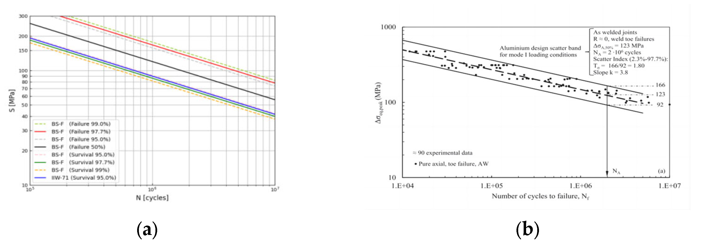
According to the welded joint classification referenced from BS7608, cruciform joints under tensile loading can be classified as category F. However, BS7608 does not provide a specific category for joints under three-point-bending loading. Considering that the material at the weld toe is indeed in the tensile stress state under three-point-bending loading, the same joint category as that under tensile loading can be adopted. In addition, BS7608 provides mean S-N curves with 50% survival probability and standard basic design S-N curves with 97.7% survival probability, shown as the black solid line and the green solid line for category F in Figure 8a, respectively. Both the S-N curves can be expressed as Equation (6), the parameters of which can be found in Table 5, together with data about other typical survival probabilities or failure probabilities. From the statistical perspective, standard basic design S-N curves are of −2 times standard deviations, which may lead to a more conservative predicted fatigue life and greater design reliability. Therefore, they are often used in practical fatigue design work. For similar reasons, design S-N curves with 95% survival probability and 75% two-sided confidence levels are provided in another widely used fatigue design recommendation, IIW. The S-N curve of category FAT71, which is similar to category F in BS7608 is shown as the blue solid line in Figure 8a. It can be observed that the two S-N curves are almost same.
l o g   N = m l o g   S + l o g   C 0 d σ
where, N is the fatigue life; S is the stress range; C0 is a constant; m is the inverse slope of the S-N curve; d is the number of standard deviations less than the mean; and σ is the standard deviation.
Nevertheless, for the damage calculation, S-N curves with higher survival probability probably result in rather bad prediction results, which can be explained by the relationship between the design S-N curve and the fatigue test data, as shown in Figure 8b. Theoretically, all the test results should lie on the upper right of the design S-N curve, indicating that the design S-N curve has remarkable fatigue reliability. Obviously, this kind of S-N curve is not appropriate for characterizing the damage condition because the points on this design S-N curve actually do not represent the states with damage value D = 1, meaning critical fatigue damage has occurred. Based on this consideration, an S-N curve with +2 times standard deviations seems more reasonable to construct the DDM, which is shown as the red solid line in Figure 8a, corresponding to the No. 2 S-N curve in Table 5.
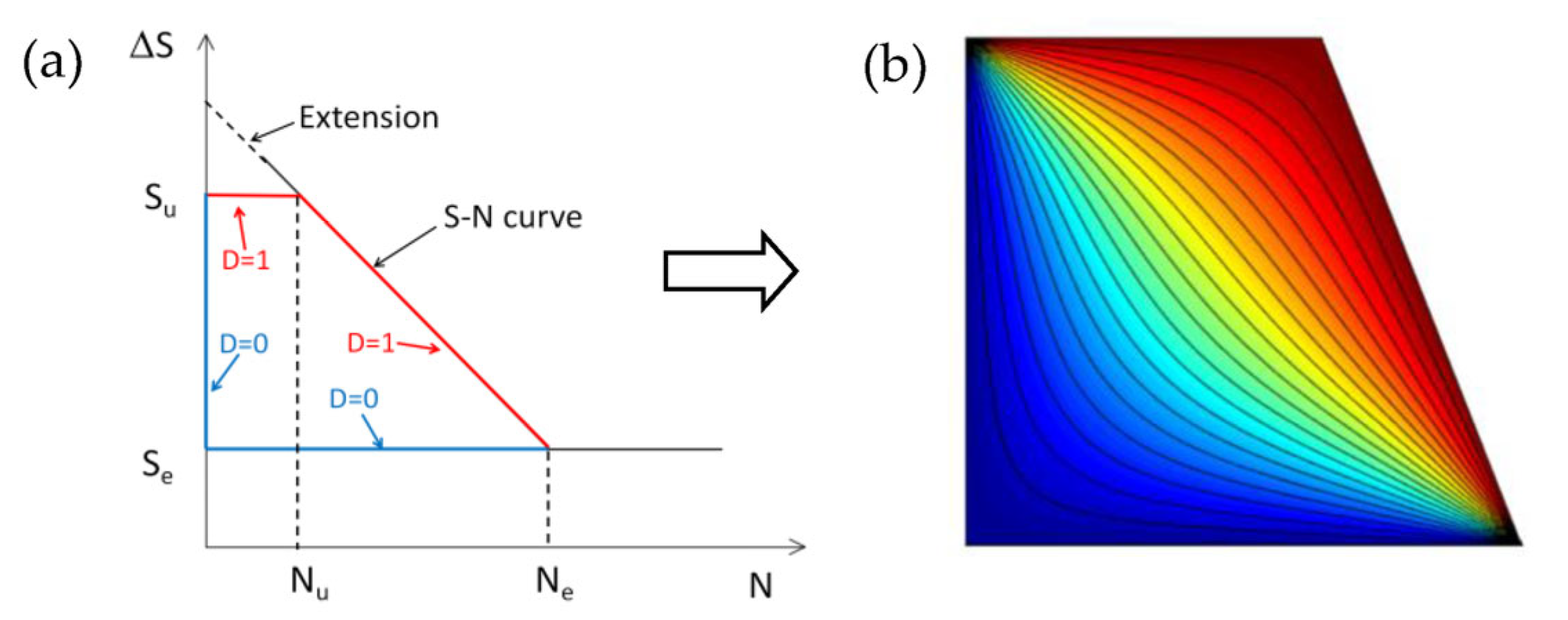
Meanwhile, from the engineering practicability aspect, most S-N curves provided in standards and codes only cover the life range of 105 to 107 cycles. Some researchers have suggested that the S-N curves could be extrapolated to the S-axis, and the intersection corresponds to the ultimate strength Su. Based on this idea, all S-N curves in Figure 8a are extended, and the extrapolated Su values are listed in Table 5. It can be observed that all the extrapolated Su values are far beyond the actual ultimate strength of commonly used metal materials. Commonly, for a ductile material bearing cyclic loads with a stress range of yield strength, failure will occur when the material only experiences a few cycles, which is indeed static damage. Based on this fact and considering the yield strength of 345 MPa according to the Q345B material from Table 5, a horizontal line corresponding to the stress range of 345 MPa is drawn and cut from the extended S-N curves in Figure 9a, and then the boundaries with damage D = 1 can be reconstructed by the horizontal line and the remaining S-N curves. Moreover, the stress range corresponding to N = 107 is defined as the fatigue limit Se in BS7608. Based on this assumption, the calculated fatigue limit Se reached 77.84 MPa using the S-N curve of category F with +2 times standard deviations, which is unreasonably high for welded structures. Further, the calculated fatigue limit Se based on the standard basic design S-N curve of category F (corresponding to the −2 times standard deviations) is 40 MPa. If S-N curves with −2 times standard deviations in IIW are used, the calculated fatigue limit Se is 32.4 MPa and 28.7 MPa for categories FAT80 and FAT71, respectively. In this paper, the fatigue life corresponding to the fatigue limit is magnified to 108 cycles, and then the calculated fatigue limit Se of category F is 36.13 MPa, which is considered reasonable and is used to reconstruct the horizontal boundary with damage D = 0. Some trial calculations were conducted according to the improved DDM shown in Figure 9 and the original DDM shown in Figure 8, showing that the former had relatively good accuracy for different load levels, while the latter was obviously unreasonable especially for small and large load levels. In total, the boundaries with damage D = 0 consist of the vertical S-axis and the newly constructed horizontal line corresponding to the calculated fatigue limit, which is shown in Figure 9a. Further, Figure 9b shows the generated DDM.

3.3. Cumulative Damage Calculation

The damage accumulation is calculated according to the test loading spectrum in Figure 8, and the results are listed in Table 6 and Table 7. In addition to the proposed damage accumulation approach, Miner’s law, the DDLR model, the Aeran model, and the Rege model are also used for comparison. The No. 2 S-N curve in Table 5 is used for the Aeran and Rege models and the proposed approach. Only the load sequence effect is considered in the damage calculation, and the effects of load type and mean stress are ignored. Assuming that the critical damage is 1, failure occurs at the 11th, 10th, 8th, and 8th loading blocks for H-L sequences and the 12th, 11th, 9th, and 9th loading blocks for L-H sequences, corresponding to the Miner, DDLR, Aeran, and Rege models, respectively. The corresponding calculated lives are 102.71 × 10⁴ cycles, 95.75 × 10⁴ cycles, 70.10 × 10⁴ cycles, and 78.65 × 10⁴ cycles for H-L sequences and 111.46 × 10⁴ cycles, 105.71 × 10⁴ cycles, 80.06 × 10⁴ cycles, and 88.65 × 10⁴ cycles for L-H sequences. In contrast, the calculated failure timing based on the proposed approach is in the 9th loading block for H-L sequences and the 10th loading block for L-H sequences, and the corresponding calculated lives are 87.81 × 10⁴ cycles for H-L sequences and 97.23 × 10⁴ cycles for L-H sequences. It can be seen that the results based on the proposed approach are in best agreement with the average test lives.
The relationship between the calculated damage and the corresponding loading cycles are plotted, as shown in Figure 10. It can be observed that Miner’s law and the DLDR model appear obviously linear, while the Aeran model, the Rege model and the proposed approach show a nonlinear tendency. It should be noted that the Aeran model not only considers the load sequence effect but also introduces load interaction factors µi [23], which can well describe the effect of the next loading block on the previous loading block with different stress ranges. However, the Aeran model seems unsuccessful in our attempt. In Figure 10, the curve based on the Aeran model shows a zigzag shape, which may result from the lack of robustness and reliability of the algorithm. In fact, during the research, we found that the Aeran model is greatly affected by the stress levels and the S-N curve parameters. Sometimes, the algorithm could not even work normally due to the negative damage value. For comparison, the results of the Aeran model were fitted, and they are shown as the red solid line in Figure 10.
An interesting phenomenon is that the calculated damage values based on Miner’s law and the DLDR model are relatively higher in the early stage of the fatigue process, while the calculated damage values based on the Aeran model, the Rege model, and the proposed approach are lower, even close to 0. Here, the definition of fatigue damage, which has been always controversial [30,31], is an issue worth pondering, especially for welded structures. Generally, the fatigue process of materials and structures can be divided into three stages, namely crack initiation, crack propagation, and final fracture [32,33]. Some researchers have argued that the term crack initiation is too academic and have further subdivided it into several sub-stages, such as microcrack nucleation, microcrack aggregation, short crack formation, short crack propagation, etc. [34,35,36,37]. It has been confirmed that the crack initiation stage occupies a large proportion of the total fatigue life. Generally, it can account for 30% to 50% for high-cycle fatigue [33,38] and even 90% for ultra-high-cycle fatigue [39,40]. In addition, the scales of the early cracks are always very small, so they are nearly impossible to be observed by traditional technological measurements. According to the damage definition based on the crack scale, the damage caused in the fatigue early stage should be very small, even close to 0.
According to the literature [37], the length of the initial cracks of welded structures can be determined as 0.1 mm rationally. Assuming that the failure states corresponding to D = 1 are cracks propagating through the plate with a thickness of 8 mm (Figure 6), the damage corresponding to crack initiation can be simply defined as D = 0.1/8 = 0.0125 ≈ 0.01. According to the test loading spectrum, loading cycles with damage values of 0.01 and 0.1 are calculated by all five models mentioned above, the results of which are listed in Table 8, where the average test life is regarded as the reference life. It can be observed that the life ratios corresponding to D = 0.01 and D = 0.1 are too small based on the Miner, DDLR, and Aeran models. Comparatively, the results of the Rege model and the proposed approach seem more reasonable. Therefore, from the view of physical mechanisms, the Rege model and the proposed approach have great advantages in characterizing the fatigue early behavior of welded structures.

3.4. Fatigue Life Prediction

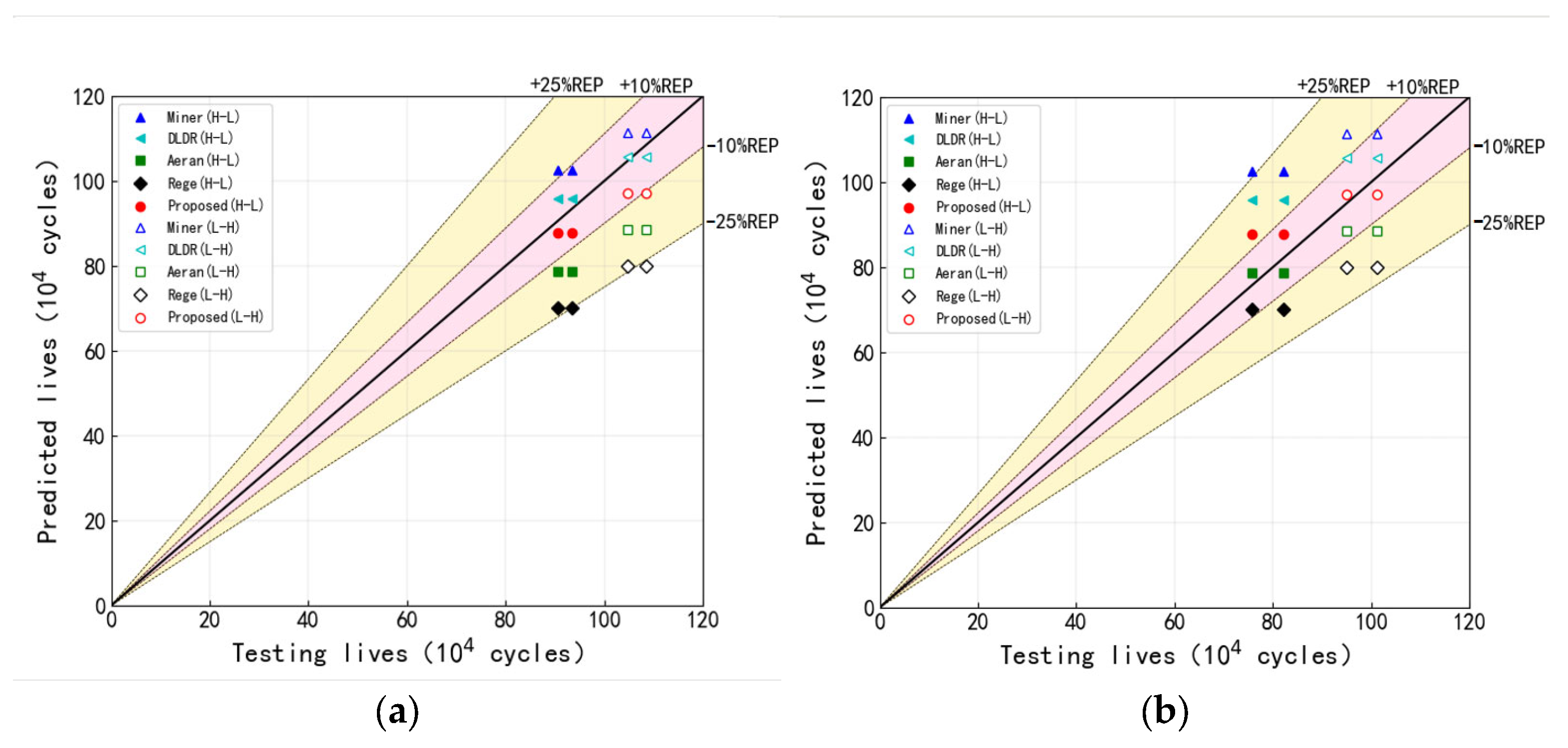
Assuming the critical damage is 1, fatigue lives are predicted. The comparison of the predicted lives with the testing lives is shown in Figure 11, among which the red area and yellow area correspond to the scatter bands with accuracy of 10% and 25% respectively. It can be seen that there are total seven red points based on the proposed approach inside the red scattered band with 10% accuracy of both (a) and (b), except only one point outside under simple tensile loading. Based on Miner, DDLR, Aeran and Rege models, the total numbers of the result points in the red scattered band of both (a) and (b) are 4, 6, 3 and 1 respectively. Therefore, the proposed model shows highest life prediction accuracy. It should be noted that, except the proposed approach, the result points based on the nonlinear models (Aeran and Rege model) are fewer than those of the linear models (Miner and DDLR model) in the red scattered band, which seems to show that linear models are better than nonlinear models except the proposed approach from the view of life prediction accuracy. However, it should be emphasized that the fatigue life here refers to the total life and the real damage evolution is not considered in its definition. If the crack evolution behavior needs to be considered, the nonlinear models especially the proposed model are of outstanding advantages.
It seems that, in Figure 11, linear models are prone to overestimating fatigue lives, and the nonlinear models, except for the proposed model, are prone to underestimating fatigue lives. Comparatively, the result points of the proposed model almost evenly lie on both sides of the diagonal, which means that the prediction accuracy of the proposed model is better than that of the other models. In addition, for the proposed model, three result points under three-point bending lie on the upper-left side of the diagonal, while all four result points under simple tensile bending and only one result point under three-point-bending lie on the lower-right side of the diagonal, which seems to show that the loading type has some influence on life prediction. This issue is worth investigating further.

4. Conclusions

In the present work, the nonlinear fatigue damage accumulation prediction for welded structures under variable amplitude loadings is investigated. The following conclusions can be drawn.
(1)
Based on Pavlou’s theory, the fatigue damage envelope for welded joints can be reasonably constructed by directly adopting S-N curves provided in welded structure fatigue design standards and codes. According to the FEA solution for a heat transfer problem, the damage distribution map can be generated, and the corresponding polynomial fitting function can be derived. Then, the cumulative damage and fatigue life for welded joints under variable amplitude loadings can be predicted.
(2)
For cruciform joints and T joints, respectively, simple tensile and three-point-bending fatigue tests under two-level loading block sequences were conducted. An S-N curve with 97.7% failure probability for F class in BS7608 was adopted, and the boundary condition corresponding to damage D = 0 of the heat transfer FEA model was set as −8 °C. The cumulative damage was calculated based on the Miner, DLDR, Aeran, and Rege models and the proposed model. The prediction results show that the proposed approach is in best agreement with the experimental results. It is interesting that nonlinear models do not seem better than linear models for overall fatigue life prediction, which may be because the overall fatigue lives ignore the dominant damage differences among different fatigue stages.
(3)
Comparison of the damage prediction results according to the five models shows that nonlinear models have significant advantages in describing the damage characteristics in the fatigue early stage of weld toe cracks. Therefore, from aspects of both life prediction accuracy and crack damage process description, the proposed model is superior to others.

Author Contributions

H.D. is responsible for writing and finalizing the version to be published. Z.D. is responsible for article data acquisition, analysis and interpretation. G.W. is responsible for the research idea design of the paper. All authors have read and agreed to the published version of the manuscript.

Funding

This research was funded by National Natural Science Foundation of China (Grant Number: 51575408); Key Technologies Research & Development Program of Hubei Province (Grant Number: 2021BAA202) and Department of Education Scientific research program guidance project of Hubei Province (Grant Number: B2022022).

Institutional Review Board Statement

Not applicable.

Data Availability Statement

Not applicable.

Conflicts of Interest

The authors declare no conflict of interest.

Nomenclature

N fatigue life S stress range
C specific heat ρ density
C 0 a constant of materialRstress ratio
d the number of standard deviation less than the mean R M S E mean square error
D damageR-Squaresquare of correlation coefficient
D Σ cumulative damage S e fatigue limit
D x , y interpolation function of damage S i stress range of loading block i
k thermal conductivity S S E sum of squares of fitting errors
m inverse slope of S-N curve S u ultimate strength
n i cycles of loading block i t time
N i life under constant amplitude loading SiTfunction of temperature
σstandard deviation μ i load interaction factor

References

  1. Łagoda, T.; Głowacka, K. Fatigue life prediction of welded joints from nominal system to fracture mechanics. Int. J. Fatigue 2020, 137, 105647. [Google Scholar] [CrossRef]
  2. Murakami, Y.; Endo, M. The reality of the concept of fatigue damage in multiple step amplitude loadings: Reason for unsuccessful results of existing damage counting models. Int. J. Fatigue 2022, 154, 106529. [Google Scholar] [CrossRef]
  3. Fernández-Canteli, A.; Castillo, E.; Blasón, S. A methodology for phenomenological analysis of cumulative damage processes. Application to fatigue and fracture phenomena. Int. J. Fatigue 2021, 150, 106311. [Google Scholar] [CrossRef]
  4. Miner, M.A. Cumulative damage in fatigue. J. Appl. Mech. 1945, 67, A159–A164. [Google Scholar] [CrossRef]
  5. Mesmacquea, G.; Garciab, S.; Amrouchea, A.; Rubio-Gonzalezb, C. Sequential law in multiaxial fatigue, a new damage indicator. Int. J. Fatigue 2005, 27, 461–467. [Google Scholar] [CrossRef]
  6. Lu, X.; Zheng, S. Changes in mechanical properties of vehicle components after strengthening under low-amplitude loads below the fatigue limit. Fatigue Fract. Eng. Mater. Struct. 2009, 32, 847–855. [Google Scholar]
  7. Marco, S.M.; Starkey, W.L. A concept of fatigue damage. Trans. ASME 1954, 76, 627–632. [Google Scholar] [CrossRef]
  8. Manson, S.S.; Halford, G.R. Practical implementation of the double linear damage rule and damage curve approach for treating cumulative fatigue damage. Int. J. Fract. 1981, 17, 169–192. [Google Scholar] [CrossRef] [Green Version]
  9. Xue, Q.; Du, X. Welding fatigue design based on nonlinear damage theory. J. Mech. Eng. 2019, 55, 32–38. [Google Scholar]
  10. Gao, K.; Liu, G.; Tang, W. An improved Manson-Halford model for multi-level nonlinear fatigue life prediction. Int. J. Fatigue 2021, 151, 106393. [Google Scholar] [CrossRef]
  11. Zhao, G.; Liu, Y.; Ye, N. An improved fatigue accumulation damage model based on load interaction and strength degradation. Int. J. Fatigue 2022, 156, 106636. [Google Scholar] [CrossRef]
  12. Miller, K.J.; Zachariah, K.P. Cumulative damage laws for fatigue crack initiation and stage I propagation. J. Strain Anal. Eng. Des. 1977, 12, 262–270. [Google Scholar] [CrossRef]
  13. Chaboche, J.L. A differential law for nonlinear cumulative fatigue damage. In Materials and Building Research; Annales de l’ITBTP, HS No. 39; Paris Institut Technique du Batiment et des Travaus Publies: Paris, France, 1974; pp. 117–124. [Google Scholar]
  14. Chaboche, J.L. Continuum damage mechanics and its application to structural lifetime predictions. La Rech. Aerosp. (Engl. Ed.) 1987, 4, 37–54. [Google Scholar]
  15. Lemaitre, J.; Chaboche, J.L. Mechanics of Solid Materials. J. Eng. Mech. 1993, 119, 642–643. [Google Scholar] [CrossRef]
  16. Wang, J. A continuum damage mechanics model for low-cycle fatigue failure of metals. Eng. Fract. Mech. 1992, 41, 437–441. [Google Scholar]
  17. Wang, T.; Lou, Z. A continuum damage model for weld heat affected zone under low cycle fatigue loading. Eng. Fract. Mech. 1990, 37, 825–829. [Google Scholar] [CrossRef]
  18. Subramanyan, S. A cumulative damage rule based on the knee point of the S-N curve. J. Eng. Mater. Technol. 1976, 98, 316–321. [Google Scholar] [CrossRef]
  19. Pavlou, D.G. A phenomenological fatigue damage accumulation rule based on hardness increasing, for the 2024-T42 aluminium. Eng. Struct. 2002, 24, 1363–1368. [Google Scholar] [CrossRef]
  20. Hectors, K.; De Waele, W. Cumulative damage and life prediction models for high-cycle fatigue of metals: A review. Metals 2021, 11, 204. [Google Scholar] [CrossRef]
  21. Muñiz-Calvente, M.; Álvarez-Vázquez, A.; Pelayo, F.; Aenlle, M.; García-Fernández, N.; Lamela-Rey, M.J. A comparative review of time-and frequency-domain methods for fatigue damage assessment. Int. J. Fatigue 2022, 163, 107069. [Google Scholar] [CrossRef]
  22. Aeran, A.; Siriwardane, S.C.; Mikkelsen, O.; Langen, I. A new nonlinear fatigue damage model based only on S-N curve parameters. Int. J. Fatigue 2017, 103, 327–341. [Google Scholar] [CrossRef]
  23. Rege, K.; Pavlou, D.G. A one-parameter nonlinear fatigue damage accumulation model. Int. J. Fatigue 2017, 98, 234–246. [Google Scholar] [CrossRef]
  24. Zhu, S.-P.; Liao, D.; Liu, Q.; Correia, J.A.; De Jesus, A.M. Nonlinear fatigue damage accumulation:Isodamage curve-based model and life prediction aspects. Int. J. Fatigue 2019, 128, 105185. [Google Scholar] [CrossRef]
  25. Hashin, Z.; Rotem, A. A cumulative damage theory of fatigue failure. Mater. Sci. Eng. 1978, 34, 147–160. [Google Scholar] [CrossRef]
  26. Pavlou, D.G. The theory of the S-N fatigue damage envelope: Generalization of linear, double-linear, and non-linear fatigue damage models. Int. J. Fatigue 2018, 110, 204–214. [Google Scholar] [CrossRef]
  27. Klesnil, M.; Lukáš, P. Influence of strength and stress history on growth and stabilisation of fatigue cracks. Eng. Fract. Mech. 1972, 4, 77–92. [Google Scholar] [CrossRef]
  28. Schijve, J. Effect of load sequences on crack propagation under random and program loading. Eng. Fract. Mech. 1973, 5, 269–280. [Google Scholar] [CrossRef]
  29. Meneghetti, G.; Campagnolo, A. State-of-the-art review of peak stress method for fatigue strength assessment of welded joints. Int. J. Fatigue 2020, 139, 105705. [Google Scholar] [CrossRef]
  30. Aeran, A.; Acosta, R.; Siriwardane, S.C.; Starke, P.; Mikkelsen, O.; Langen, I.; Walther, F. A nonlinear fatigue damage model: Comparison with experimental damage evolution of S355 (SAE 1020) structural steel and application to offshore jacket structures. Int. J. Fatigue 2020, 135, 105568. [Google Scholar] [CrossRef]
  31. Bjørheim, F.; Siriwardane, S.C.; Pavlou, D. A review of fatigue damage detection and measurement techniques. Int. J. Fatigue 2022, 154, 106556. [Google Scholar] [CrossRef]
  32. Leonetti, D.; Maljaars, J.; Snijder, H.H.B. Fracture mechanics based fatigue life prediction for a weld toe crack under constant and variable amplitude random block loading—Modeling and uncertainty estimation. Eng. Fract. Mech. 2021, 242, 107487. [Google Scholar] [CrossRef]
  33. Remes, H.; Gallo, P.; Jelovica, J. Fatigue strength modelling of high-performing welded joints. Int. J. Fatigue 2020, 135, 105555. [Google Scholar] [CrossRef]
  34. Haghshenas, A.; Khonsari, M.M. Damage accumulation and crack initiation detection based on the evolution of surface roughness parameters. Int. J. Fatigue 2018, 107, 130–144. [Google Scholar] [CrossRef]
  35. Guerchais, R.; Saintier, N.; Morel, F.; Robert, C. Micromechanical investigation of the influence of defects in high cycle Fatigue. Int. J. Fatigue 2014, 67, 159–172. [Google Scholar] [CrossRef] [Green Version]
  36. Schork, B.; Kucharczyk, P.; Madia, M.; Zerbst, U.; Hensel, J.; Bernhard, J.; Tchuindjang, D.; Kaffenberger, M.; Oechsner, M. The effect of the local and global weld geometry as well as material defects on crack initiation and fatigue strength. Eng. Fract. Mech. 2018, 198, 103–122. [Google Scholar] [CrossRef]
  37. Yıldırım, H.C.; Remes, H.; Nussbaumer, A. Fatigue properties of as-welded and post-weld-treated high-strength steel joints: The influence of constant and variable amplitude loads. Int. J. Fatigue 2020, 138, 105687. [Google Scholar] [CrossRef]
  38. Zerbst, U.; Hensel, J. Application of fracture mechanics to weld fatigue. Int. J. Fatigue 2020, 139, 105801. [Google Scholar] [CrossRef]
  39. Raftar, H.R.; Dabiri, E.; Ahola, A.; Björk, T. Weld root fatigue assessment of load-carrying fillet welded joints: 4R method compared to other methods. Int. J. Fatigue 2022, 156, 106623. [Google Scholar] [CrossRef]
  40. Rozumek, D.; Lewandowski, J.; Lesiuk, G.; Correia, J.A. The influence of heat treatment on the behavior of fatigue crack growth in welded joints made of S355 under bending loading. Int. J. Fatigue 2020, 131, 105328. [Google Scholar] [CrossRef]
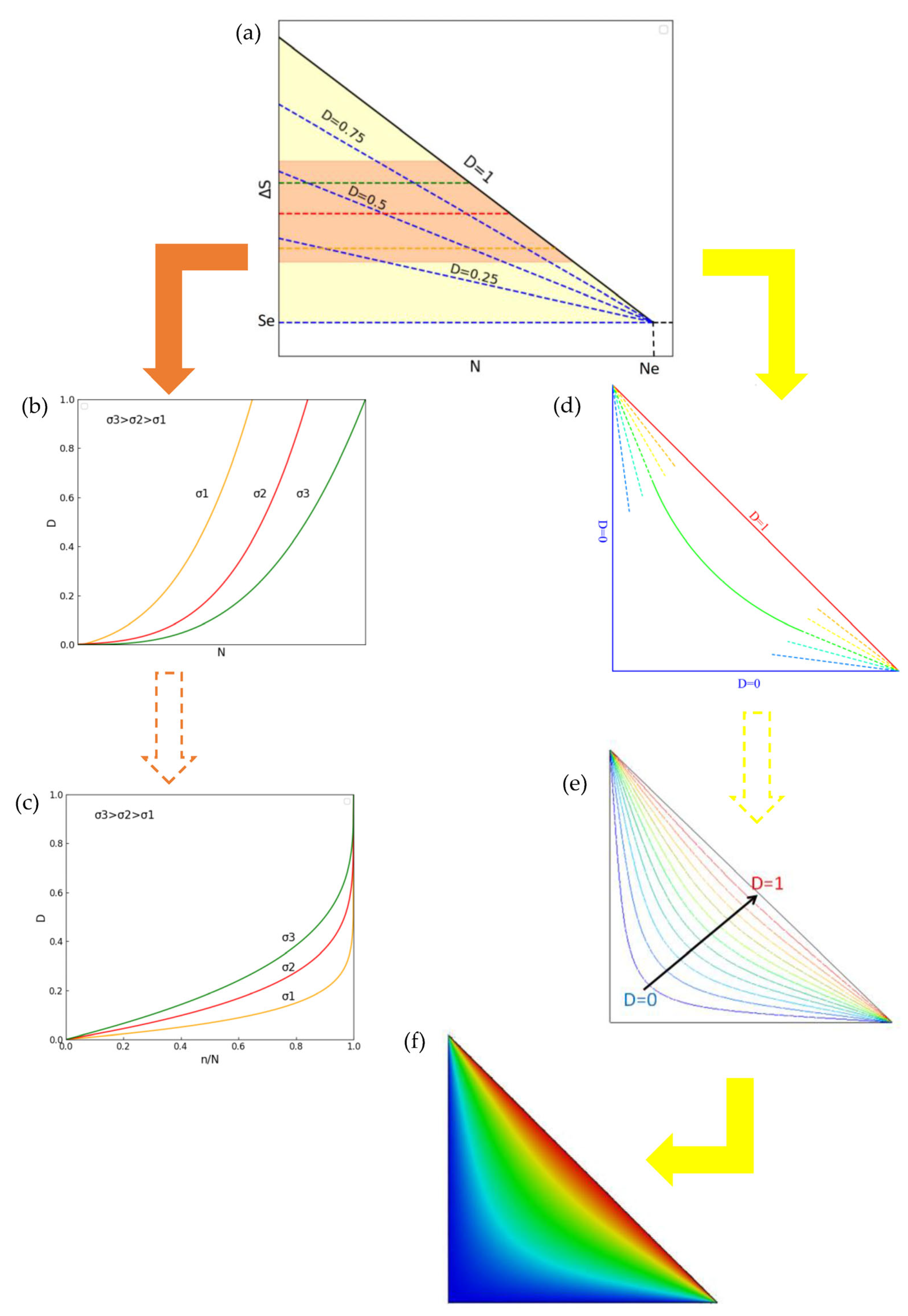
Figure 1. Schematic diagram of DDM concept. (a) S-N curve; (b) isostress curves with normal N-axis; (c) isostress curves with normalized N-axis; (d) isodamage curve converging to both N-axis and S-axis; (e) isodamage curves ranging from 0 to 1; (f) damage distribution map.
Metals 13 01203 g001
Figure 2. Analysis model of heat transfer problem.
Metals 13 01203 g002
Figure 3. DDM and extracted isodamage curves.
Metals 13 01203 g003
Figure 4. Comparison of 3D DDM. (a) From FEA (nodes typed); (b) from interpolation (surfaces typed).
Metals 13 01203 g004
Figure 5. Flow chart of the proposed approach.
Metals 13 01203 g005
Figure 6. Geometry and dimension of specimens (mm).
Metals 13 01203 g006
Figure 7. Loading block sequences for tests. (a) H-L with R = 0 for L-level loading blocks; (b) H-L with R = 0.5 for L-level loading blocks; (c) L-H with R = 0 for L-level loading blocks; (d) L-H with R = 0.5 for L-level loading blocks.
Metals 13 01203 g007
Figure 8. S-N curves for weld joints. (a) For category F used in this paper; (b) with 180 test data based on peak stress method [29].
Metals 13 01203 g008
Figure 9. Construction of DDM for welded joints. (a) Heat transfer analysis model; (b) generated DDM.
Metals 13 01203 g009
Figure 10. Calculated damage evolution process. (a) H-L loading sequences; (b) L-H loading sequences.
Metals 13 01203 g010
Figure 11. Comparison of predicted lives and testing lives.
Metals 13 01203 g011
Table 1. Mechanical properties of Q345B steel.
Yield Strength
σ s
Ultimate Tensile Strength
σ b
Elongation
(%)
Young’s Modulus
E (Mpa)
Poisson’s Ratio
μ
358564≤22.32.08 × 1050.31
Table 2. Chemical compositions of Q345B steel (wt.%).
CSiMnPS
0.1500.3801.3600.0300.028
Table 3. Welding parameters.
Welding Current
I (A)
Welding Voltage
U (V)
Welding Speed
v   ( mm · s 1 )
GasGas Flow Rate
Q   ( L · min 1 )
240250.8Ar-20%CO220
Table 4. Testing lives and corresponding parameters.
No. of SpecimensTesting Lives (104 Cycles)Loading Spectrum TypeMemo
C0110 + 10 + 10 + 10 + 10 + 10 + 10 + 10 + 10 + 0.5=90.5a (H-L)cruciform joint specimens under simple tensile loading
C0210 + 10 + 10 + 10 + 10 + 10 + 10 + 10 + 10 + 3.4=93.4b (H-L)
C0310 + 10 + 10 + 10 + 10 + 10 + 10 + 10 + 10 + 10 + 8.4=108.4c (L-H)
C0410 + 10 + 10 + 10 + 10 + 10 + 10 + 10 + 10 + 10 + 4.7=104.7d (L-H)
T0110 + 10 + 10 + 10 + 10 + 10 + 10 + 10 + 2.1=82.1a (H-L)T joint specimens under three-point-bending loading
T0210 + 10 + 10 + 10 + 10 + 10 + 10 + 5.8=75.8b (H-L)
T0310 + 10 + 10 + 10 + 10 + 10 + 10 + 10 + 10 + 4.9=94.9c (L-H)
T0410 + 10 + 10 + 10 + 10 + 10 + 10 + 10 + 10 + 10 + 1.3=101.3d (L-H)
Table 5. Parameters of the used S-N curves.
No.mC0LogC0dFailure
Probability
Extrapolated Su (MPa)Standard
135.56 × 101212.742.3399.0%17,712
2 *34.72 × 101212.672.0097.7%16,771
333.95 × 101212.601.6595.0%15,802
431.73 × 101212.240.0050.0%11,995BS7608
537.55 × 101111.88−1.655.0%9106
636.32 × 101111.80−2.002.3%8580
735.36 × 101111.73−2.331.0%8124
837.16 × 101111.85/50.0% (with 75% two-sided confidence level)8945IIW
Table 6. Damage accumulation calculation results for H-L loading sequences.
Block No.MinerDLDRAeranRegeProposed
10.16960.16960.04111.39 × 10−67.06 × 10⁻⁷
20.19080.18980.18614.95 × 10−68.86 × 10⁻⁷
30.36040.35250.09722.79 × 10−43.01 × 10⁻⁵
40.38160.37530.49549.98 × 10−45.03 × 10⁻⁵
50.55120.54670.18380.0129 0.0008
60.57240.59931.60440.0471 0.0021
70.74200.76520.48390.3218 0.0277
80.76320.86551 *1.19430.0987
90.93290.9786//1 *
100.95411.0328///
111.1237////
Lives
(104 cycles)
102.7195.7570.1078.6587.81
Table 7. Damage accumulation calculation results for L-H loading sequences.
Block No.MinerDLDRAeranRegeProposed
10.02120.02120.00402.03 × 10−371.17 × 10⁻⁸
20.19080.44130.04231.39 × 10−68.21 × 10⁻⁷
30.21200.48520.19224.95 × 10−61.03 × 10⁻⁶
40.38160.62650.09902.79 × 10−43.38 × 10⁻⁵
50.40280.65900.50689.98 × 10−45.80 × 10⁻⁵
60.57240.76890.18690.0129 0.0009
70.59360.78861.74520.0471 0.0024
80.76320.86230.52590.3218 0.0306
90.78440.91551 *1.1943 0.1177
100.95410.9735//1 *
110.97531.0091///
121.1449////
Lives
(104 cycles)
111.46105.7180.0688.6597.23
Table 8. Life prediction results for specific damage.
DamagePredicted Lives (104 Cycles)/Life Ratio (%)
MinerDLDRAeranRege Proposed
H-LD = 0.010.59/0.69%0.59/0.69%2.64/3.09%48.89/57.19%50.11/58.62%
D = 0.15.89/6.89%5.89/6.89%20.98/24.54%63.75/74.58%80.02/93.61%
L-HD = 0.014.71/4.60%4.71/4.60%2.52/2.46%58.89/57.55%75.56/73.84%
D = 0.114.65/14.32%10.28/14.32%20.01/19.55%73.75/72.07%89.34/87.31%
Disclaimer/Publisher’s Note: The statements, opinions and data contained in all publications are solely those of the individual author(s) and contributor(s) and not of MDPI and/or the editor(s). MDPI and/or the editor(s) disclaim responsibility for any injury to people or property resulting from any ideas, methods, instructions or products referred to in the content.