Article

A Finite Volume-Based Unified Transient Deterministic Framework for Lubrication Modelling


1
Department of Mechanical Engineering, Imperial College London, Exhibition Road, South Kensington, London SW7 2AZ, UK
2
Department of Mechanical Engineering, University of Bath, Claverton Down, Bath BA2 7AY, UK
*
Author to whom correspondence should be addressed.
Lubricants 2026, 14(7), 281; https://doi.org/10.3390/lubricants14070281
Submission received: 3 June 2026 / Revised: 10 July 2026 / Accepted: 15 July 2026 / Published: 21 July 2026
(This article belongs to the Special Issue Modeling and Simulation of Elastohydrodynamic Lubrication)

Abstract

A unified transient deterministic lubrication model is developed for the analysis of rough, starved, and coated contacts within a single, fully-coupled numerical framework capable of resolving boundary, mixed, and full-film lubrication regimes. The model is formulated with the finite volume method on a curvilinear grid and extends conventional full-film formulations through the introduction of a semi-system methodology, enabling robust treatment of complex multi-regime conditions. A key distinguishing feature of the framework is the direct resolution of thermal effects within both the lubricant and solid domains through solution of the energy equation. Unlike many existing mixed lubrication models that rely on analytical temperature approximations, the present approach captures transient, asperity-scale temperature evolution explicitly, allowing accurate representation of local thermo-mechanical interactions. Two case studies are presented to demonstrate the capabilities of the model. The first examines transient starvation in rough contacts with isotropic sinusoidal topographies of varying wavelength, as well as random machined surfaces, revealing a strong dependence of lubricant entrainment, asperity interaction, and localised heating on surface morphology. The second study investigates the role of coating thermal properties under transient starved conditions, demonstrating strong coupling between heat transport, viscosity variations, and frictional response. Overall, the proposed framework provides a robust and physically consistent platform for the simulation of transient lubrication phenomena under realistic operating conditions, enabling detailed insight into roughness, starvation, and thermal effects across regimes using a fully-coupled approach.

1. Introduction

Elastohydrodynamic lubrication (EHL) plays a central role in the performance and durability of heavily loaded machine elements such as gears, bearings, and other rolling-sliding contacts [1]. Over the past few decades, significant progress has been made in the development of numerical models capable of predicting pressure, film thickness and friction under a wide range of operating conditions. In particular, the introduction of fully-coupled thermal frameworks and advanced numerical methods, such as finite element and finite volume approaches, has enabled increasingly accurate simulations of EHL contacts, including the effects of non-Newtonian rheology and heat generation within the lubricant and solid bodies [2].
Early numerical developments primarily focused on smooth surfaces and steady-state, fully-flooded conditions [3]. However, it is now well established that real engineering contacts operate under far more complex conditions, where surface roughness, transient effects, thermal phenomena and lubricant starvation can all play a significant role. As a result, a large body of research has emerged addressing these individual effects [1,2].
Several studies have investigated the transient passage of surface features through EHL contacts, showing that asperities can induce strong local variations in pressure, film thickness and temperature. One of the earliest studies on deterministic rough surfaces by Lubrecht et al. [4] investigated the effect of amplitude, wavelength and orientation of rough surface features on circular EHL contacts, demonstrating that the results obtained from deterministic consideration of roughness can be substantially different to those predicted using statistical methods like Patir and Cheng’s flow factor model [5,6]. Venner and Lubrecht further demonstrated the capability of numerical simulations to resolve the transient propagation of roughness features through a contact, providing key physical insights into the underlying mechanisms governing pressure and film thickness fluctuations [7]. The pioneering studies by Zhu and Hu [8,9] subsequently proposed a unified deterministic framework capable of simulating the entire transition from full-film to boundary lubrication conditions using only the Reynolds equation to calculate both hydrodynamic and asperity pressure contributions.
Concurrently, novel numerical algorithms were incorporated into such frameworks to improve their computational efficiency. For example, the multigrid method implemented by Venner and Lubrecht [10] addresses the relatively slow convergence speed of direct iterative relaxation procedures. The discrete convolution and fast Fourier transform (DC-FFT) algorithm by Liu et al. [11] improves the calculation efficiency of surface deformations while more recent techniques like progressive mesh densification [12,13] also offer significant improvements on computational speed, especially for thicker lubricant films.
Thermal effects in lubricated contacts were initially studied using analytical approaches based on frictional heating and heat conduction. Early work by Blok [14] and Jaeger [15] introduced the concept of flash temperature rise at the contact surface while the work of Carslaw and Jaeger [16] introduced the theory of a point heat source moving on the surface of a half-space solid body. These models formed the basis for many early thermal EHL (TEHL) analyses, where temperature rise was estimated using simplified analytical formulations rather than solving the full energy equation. Recent studies have extended these approaches to include transient operating conditions, surface roughness and non-Newtonian effects [17,18]. However, such studies still estimate the surface temperatures using analytical methods. In parallel, significant progress has been made towards fully-coupled TEHL formulations in which the energy equation is solved directly in both the lubricant and solid domains. Habchi et al. [19] developed a TEHL model based on a finite element framework, demonstrating the importance of accurately capturing thermal effects for reliable prediction of physical contact behaviour. More recent studies have extended such TEHL analyses by incorporating surface roughness, texturing and coating effects [20,21,22]. These works have shown that such effects can significantly influence friction and film formation. In most cases, however, asperity contact is not explicitly resolved and individual asperity interactions are not accounted for when solving the energy equations.
With regard to lubricant starvation, this is now recognised as a common operating condition in important components, such as high-speed rolling-element bearings [23]. Starvation often arises unintentionally due to insufficient oil supply or redistribution of lubricant within the system. Experimental studies have shown that even small variations in available lubricant volume can significantly alter frictional behaviour and transition the contact toward mixed lubrication regimes, strongly affecting component life and efficiency [24]. Starvation effects are also closely linked to operating conditions such as entrainment speed, surface finish, and contact geometry, and can lead to markedly different tribological responses depending on the initial lubricant distribution and surface structure [18].
Transient starvation has been studied in smooth EHL contacts where time-dependent inlet boundary conditions and lubricant supply limitations are considered. Recent contributions have demonstrated the importance of starvation dynamics on film thickness and friction evolution [25]. However, these models are generally restricted to smooth surfaces and full-film lubrication regimes, without considering deterministic surface roughness or asperity interactions.
Other models have extended the analysis to rough surfaces [26]. For example, studies considering roughness effects under starved conditions have shown that cavitation is more pronounced in textured or dented surfaces under starved lubrication regimes [27]. Additional investigations into rough surface interactions under starvation have also demonstrated that surface finish plays a critical role in determining frictional behaviour and lubrication efficiency, with different roughness structures leading to distinct starvation responses [28]. However, these formulations typically neglect thermal effects and do not resolve asperity-level contact interactions.
The importance of starvation has also been highlighted in more complex geometries and operating conditions. For example, in elliptical and circular EHL contacts, it has been shown that the lubricant inlet layer thickness governs a transition towards a quasi-fully-flooded regime, where further increases in lubricant supply have diminishing influence on film formation [29]. In finite line contacts such as gears and bearings, starvation has been shown to strongly influence friction, film thickness and fatigue life, with pronounced sensitivity to operating speed and slide-to-roll ratio [30]. Similarly, other studies of rolling bearings demonstrate that starvation not only affects film thickness, but also alters contact forces and the dynamic stability of the system [31]. These findings highlight that starvation is inherently coupled with system dynamics and cannot be treated as a purely inlet-boundary phenomenon.
Further developments have introduced thermal coupling and asperity contacts within starved EHL systems. In particular, models incorporating rough surfaces, thermal effects and asperity interactions have demonstrated the strong coupling between temperature rise and film reduction in starved conditions [32]. These studies show that the presence of roughness significantly intensifies local heating at asperity contacts, which in turn accelerates film thinning and promotes inter-asperity cavitation, particularly under reduced inlet supply conditions. Nevertheless, such approaches commonly rely on simplified thermal treatments, where the solid-body temperature evolution is estimated using analytical flash temperature formulations rather than solving the full energy equation within the solids. As a result, the spatial and transient evolution of temperature within the solid bodies cannot be fully resolved, limiting the ability to capture subsurface thermal gradients and their influence on local contact conditions.
Surface coatings have also received considerable attention, due to their ability to modify both mechanical compliance and thermal behaviour of EHL contacts [33]. Previous studies have demonstrated that coating thickness, elastic modulus, and thermal inertia significantly influence pressure distribution, film thickness, and frictional response. For instance, coated EHL contacts have been analysed under both mechanical and thermal variations, showing clear sensitivity to material properties [34]. However, most existing coating models for counterformal point contacts are limited to steady-state conditions, with transient effects not widely addressed within a fully-coupled thermal framework.
Although these phenomena, namely transient starvation, deterministic roughness, thermal asperity interactions and coatings, have been studied individually, they are rarely considered within a single unified modelling framework. In particular, existing approaches tend to separate full-film, mixed and boundary lubrication regimes, or simplify thermal effects at asperity level, limiting their applicability to realistic operating conditions.
Furthermore, the studies mentioned above predominantly employ either the finite difference method (FDM) or the finite element method (FEM) to discretise the governing equations. FDM-based approaches have been widely adopted in EHL due to their relatively straightforward implementation and computational efficiency, particularly for Reynolds equation-based formulations and unified mixed lubrication models [17,18,35]. FEM formulations, by contrast, are particularly effective for strongly coupled thermo-mechanical problems involving complex geometries and non-linear material behaviour due to their geometric flexibility and robust treatment of continuum mechanics [34]. Comparatively fewer studies have explored the finite volume method (FVM) for solving TEHL problems, despite its particular suitability for transient multiphysics transport problems. Unlike the FDM, which discretises differential operators directly at nodal locations, the FVM integrates the governing conservation laws over finite control volumes and enforces local conservation through the balance of fluxes across control-volume faces [36,37]. This ensures that the transported properties are conserved locally within each computational cell, making the FVM particularly well suited to the conservative transport equations encountered in lubrication systems. Existing FVM-based EHL studies [38,39,40] are generally limited to smooth full-film conditions and rarely incorporate deterministic roughness, asperity interactions, starvation or unified mixed lubrication formulations. Hansen et al. [41] employed an FVM framework to investigate textured ball-on-disc contacts under transient operating conditions, although their study was limited to isothermal conditions and did not consider starvation. More recently, Ardah et al. [42] combined the geometric flexibility of FEM with the conservation properties of FVM through an Element-based Finite Volume Method (EbFVM) for multiphysics transport in textured journal bearings. However, deterministic asperity interactions, transient rough-surface evolution, starvation, multilayer coatings, and fully-coupled thermo-hydrodynamic effects remained beyond the scope of those studies.
As a result, there remains a need for a comprehensive numerical model capable of simultaneously capturing transient behaviour, deterministic surface roughness, asperity-scale thermal effects, lubricant starvation and coating behaviour within a unified formulation.
In this work, a transient deterministic unified lubrication model is developed within a FVM framework on a curvilinear grid. The formulation extends previous full-film thermal EHL solvers [43,44] to a unified treatment of boundary, mixed and full-film lubrication regimes through the use of a semi-system approach [35], enabling robust and consistent solution behaviour across contact conditions. In contrast to most existing unified mixed lubrication models, the present approach employs a fully-conservative FVM framework capable of consistently resolving coupled flow and thermal transport within the lubricant, coatings and solid domains.
Building on this framework, several key advancements are introduced. First, asperity-scale thermal effects are directly resolved through the solution of the energy equation in both the lubricant and solid domains, allowing the transient temperature distribution within the contacting bodies to be captured without reliance on analytical approximations such as Carslaw-Jaeger theory. Second, the model takes into consideration the transient behaviour of systems with surface coatings, enabling the analysis of layered materials under realistic operating conditions. Finally, transient lubricant starvation is considered in combination with deterministic surface roughness and asperity contacts, a capability that, to the authors’ knowledge, has not previously been reported.

2. Methodology

2.1. Coupled Thermo-Hydrodynamic Lubrication Framework

The unified multiphysics lubrication framework developed in this study builds upon the steady-state thermal lubrication formulations previously proposed in [43,44] for both line and point contact configurations. These earlier models incorporated mass-conserving cavitation algorithms and were extensively validated against experimental measurements and high-fidelity CFD simulations, demonstrating excellent predictive capability in the evaluation of pressure, temperature, film thickness, and friction under steady-state conditions for smooth lubricated interfaces. The present contribution extends these formulations to transient rough surface lubrication problems involving deformable coated interfaces. In particular, the framework enables the fully-coupled interaction between deterministic surface topography, hydrodynamic flow, thermal transport, cavitation, and asperity contact to be resolved within a unified computational setting. This provides a rigorous and consistent description of lubrication behaviour under highly transient operating conditions, where local asperity interactions, lubricant starvation, and coating-induced thermal effects may strongly influence the interfacial response. This is achieved through a semi-system formulation [35,45], whereby the governing equations remain valid throughout the entire computational domain, including regions of vanishing film thickness corresponding to asperity contact. Consequently, the transition between full-film lubrication and asperity contact is captured implicitly, without the need for separate contact models or artificial switching criteria between lubrication regimes. This unified treatment enhances numerical robustness and enables a consistent description of lubrication behaviour across hydrodynamic, mixed, and boundary lubrication regimes.
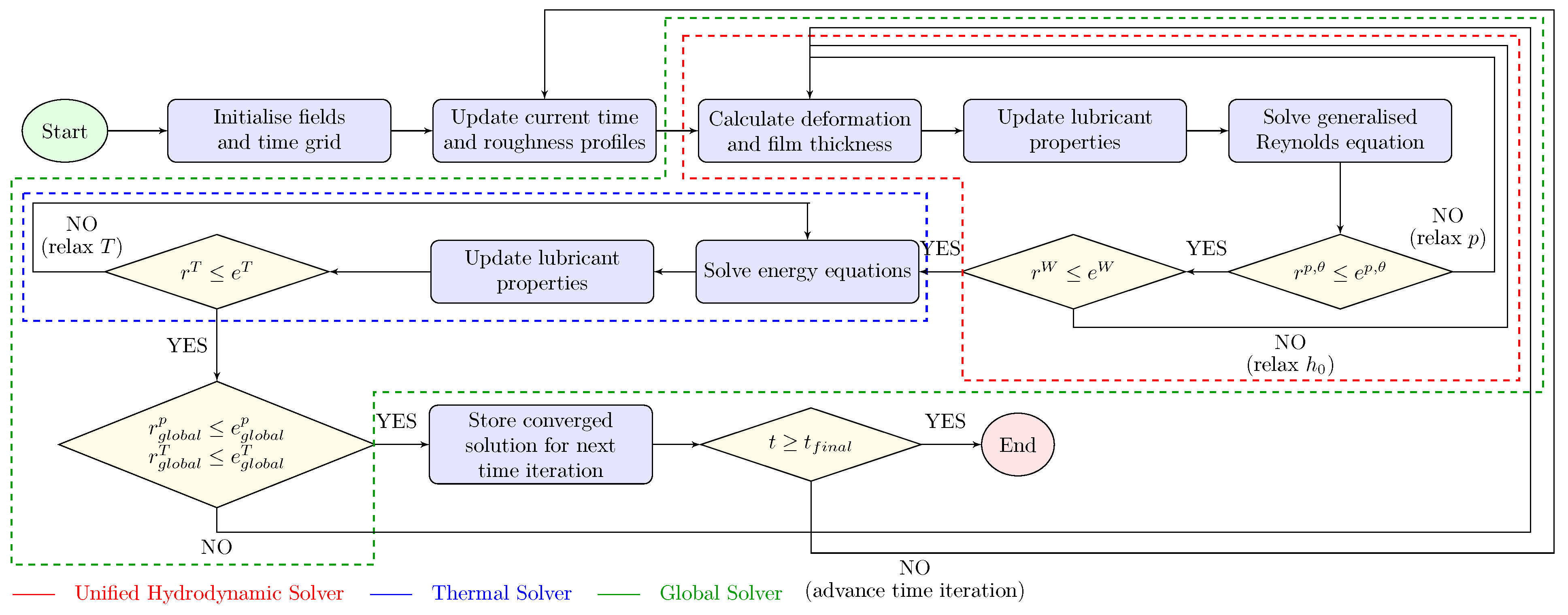
As shown in Figure 1, the solution procedure is based on a fully-coupled time-marching algorithm in which the governing equations are solved sequentially within each discrete time step while preserving the strong coupling between hydrodynamic, thermal, and interfacial phenomena. At the beginning of the simulation ( t = 0 ), the temporal discretisation is defined and the primary field variables, including pressure, temperature, film thickness, and lubricant film fraction, are initialised. During each subsequent time increment, the rough surface topography is advanced through the computational domain either by spatial translation or through a progressive evolution of the roughness amplitude, thereby enabling transient rough surface interactions to be captured explicitly. Within each time step, the coupled lubrication problem is solved iteratively through a global non-linear solution loop. The isothermal lubrication problem is solved first in order to obtain converged pressure, lubricant film fraction, and film thickness distributions satisfying the externally applied load. Convergence of the hydrodynamic solution is achieved when the combined pressure-film fraction residual, r p , θ , falls below the prescribed convergence tolerance, e p , θ . Simultaneously, load equilibrium is enforced through the load residual r W , which must satisfy the convergence criterion e W .
Once hydrodynamic convergence has been achieved, the thermal problem is solved using the converged pressure and film thickness fields. The energy equations governing the lubricant film, coating layers, and solid domains are solved iteratively until the temperature residual r T becomes smaller than the thermal convergence tolerance e T . Following thermal convergence, the global pressure and temperature residuals, r global p and r global T , are evaluated to assess convergence of the fully-coupled multiphysics system. Global convergence for a given time step is achieved once both residuals satisfy their corresponding tolerances, e global p and e global T . The converged solution is subsequently stored and used to initialise the following time step. This introduces the required temporal continuity and history dependence necessary for resolving transient thermo-hydrodynamic and asperity-scale phenomena. The solution procedure is then repeated until the final simulation time is reached.
The residual measures employed throughout the solution procedure are defined as follows:
r p , θ = i = 1 N x j = 1 N y p i , j n p i , j n 1 i = 1 N x j = 1 N y p i , j n + i = 1 N x j = 1 N y θ i , j n θ i , j n 1 i = 1 N x j = 1 N y θ i , j n ,
r W = W Ω p ( x , y ) d x d y W ,
r T = i = 1 N x j = 1 N y k = 1 N z T i , j , k n T i , j , k n 1 i = 1 N x j = 1 N y k = 1 N z T i , j , k n ,
r global p = i = 1 N x j = 1 N y p i , j g p i , j g 1 i = 1 N x j = 1 N y p i , j g ,
r global T = i = 1 N x j = 1 N y k = 1 N z T i , j , k g T i , j , k g 1 i = 1 N x j = 1 N y k = 1 N z T i , j , k g .
Here, i, j, and k denote the nodal indices in the x-, y-, and z-directions, respectively, while N x , N y , and N z correspond to the number of discretisation points along each coordinate direction. The superscript n denotes the current iteration within the hydrodynamic or thermal sub-solvers, whereas g denotes the iteration level associated with the global coupled solution procedure.

2.1.1. Hydrodynamic Flow and Mass Conservation

The hydrodynamic behaviour of the confined lubrication film is described using the generalised Reynolds equation that accounts for spatiotemporal variations in film thickness h ( x , y , t ) , lubricant viscosity η ( x , y , t ) , and density ρ ( x , y , t ) , together with the kinematics of the bounding surfaces [46]. The latter are defined by the velocity fields v 1 = u 1 v 1 T and v 2 = u 2 v 2 T in the x- and y-directions pertaining to the lower and upper surfaces, respectively. To ensure a physically consistent treatment of lubricant rupture and reformation, a mass-conserving p θ formulation based on the Elrod-Adams cavitation algorithm is employed [47,48,49]. This approach enforces the Jakobsson-Floberg-Olsson (JFO) complementary conditions [50,51], enabling a robust description of pressurised and cavitated regions within the lubricated domain. Accordingly, the coupled pressure-film fraction ( p θ ) form of the generalised Reynolds equation (GRE) is expressed in conservative form as follows:
x ε p x + y ε p y Pressure flow terms = ( θ ρ x * ) x + ( θ ρ y * ) y Entraining flow terms + ( θ ρ e ) t Transient term .
The effective transport coefficients in Equation (2) that take into account the variations of viscosity and density across the film thickness are defined as follows:
ε = η e η e ρ ρ , ρ x * = ρ e u 1 + η e u s ρ , ρ y * = ρ e v 1 + η e v s ρ , ρ e = z 1 z 2 ρ d z , 1 η e = z 1 z 2 d z η , ρ = z 1 z 2 ρ z 1 z d z η d z , 1 η e = z 1 z 2 z d z η , ρ = z 1 z 2 ρ z 1 z z d z η d z .
Additionally, the coexistence of pressurised and cavitated regions is governed by a set of complementarity conditions which enforces the mutually exclusive states as follows:
( p p c a v ) ( 1 θ ) = 0 p > p c a v θ = 1 ( fully - flooded ) , p = p c a v 0 θ < 1 ( cavitated region ) ,
where p cav denotes the cavitation pressure, while θ = ρ / ρ c represents the fluid fraction, with ρ c corresponding to the density of the saturated lubricant at cavitation conditions.
This formulation naturally extends to the modelling of inlet starvation by prescribing the film fraction at the inlet as a function of the available lubricant supply. Specifically, the film fraction is defined through the ratio of the lubricant thickness h oil to the local geometric film thickness h, such that:
θ = h oil h .
Here, h oil represents the thickness of lubricant available at the inlet, thereby limiting the local film formation when θ < 1 . This approach provides a physically consistent and mass-conserving representation of starvation within the p θ framework, without the need for additional boundary conditions or empirical corrections.
The finite volume discretisation of the GRE as well as the energy equations for the fluid and solid bodies can be found in Appendix B.

2.1.2. Deterministic Representation of Surface Roughness

Surface roughness is incorporated using a fully-deterministic framework based on the approach of Hu and Zhu [9], in which the roughness field is explicitly resolved within the governing equations, rather than treated through stochastic or homogenised approximations. Within this formulation, the generalised Reynolds equation is applied consistently across the entire computational domain to capture both hydrodynamic pressure generation in regions of finite film thickness ( h > 0 ) and contact pressure in regions where the lubricant film collapses ( h 0 ). The transition between these regimes is handled implicitly through a local modification of the governing equation, thereby avoiding the need for separate contact models or domain decomposition.
In regions where a continuous lubricant film is present, the full form of the generalised Reynolds equation (Equation (2)) is retained. However, when the local film thickness approaches zero, the pressure-driven (Poiseuille) flow contribution becomes negligible. In such cases, the governing equation reduces to the following form:
( θ ρ x * ) x + ( θ ρ y * ) y + ( θ ρ e ) t = 0 ,
which represents a balance between entrainment and transient mass transport in the absence of pressure-driven flow.
On the other hand, in asperity contact regions where the film thickness is locally constant (i.e., negligible spatial gradients), the transient contribution becomes insignificant, leading to the following simplified form:
( θ ρ x * ) x + ( θ ρ y * ) y = 0 ,
which describes purely advective transport along the lubricated interface.
Therefore, the appropriate form of the governing equation is selected locally based on the relative magnitude of the film thickness and its spatial gradient. Specifically, the following criteria are employed:
Hydrodynamic   governing   equation Equation ( 2 ) , if h a > ε h , Equation ( 5 ) , if h a < ε h , and h x > ε s , Equation ( 6 ) , if h a < ε h , and h x < ε s ,
where a denotes the characteristic length scale of the contact (taken here as the Hertzian contact radius), while ε h = 10 6 and ε s = 10 5 are the prescribed numerical tolerances used to distinguish between full-film, transition, and asperity contact regimes. These thresholds are chosen to ensure numerical robustness while maintaining a physically consistent identification of regions with diminishing lubricant film thickness and negligible surface gradients.
These conditions are evaluated locally during every time step, enabling a fully-transient and spatially-resolved treatment of rough surface interactions. This local and dynamic adaptation of the governing equations ensures that hydrodynamic and contact responses are captured consistently and simultaneously within a single computational framework, without the need for predefined regime separation. The simulation is initialised using a smooth surface solution, which provides a numerically stable baseline for the subsequent deterministic evolution of the roughness field. As the simulation progresses, the rough surface is advected through the computational domain, allowing the time-dependent interaction between surface topography, lubricant flow, and interfacial contact to be resolved explicitly. This approach is adopted in order to capture of transient phenomena arising from asperity-scale interactions, including localised film collapse, pressure redistribution, and the intermittent formation of contact regions. As such, the framework provides a physically consistent description of lubrication behaviour in rough interfaces, beyond the limitations of homogenised or stochastic roughness models.

2.1.3. Film Thickness and Interface Deformation

The local geometry of the lubricant film is described by a coupled representation that accounts for macroscopic surface curvature, elastic deformation, and time-dependent surface roughness. For a point contact configuration, the film thickness distribution is expressed in Cartesian coordinates as follows:
h ( x , y , t ) = h 0 + x 2 2 R x + y 2 2 R y + δ ( x , y ) + s 1 ( x , y , t ) + s 2 ( x , y , t ) ,
where h 0 denotes the rigid body separation, and R x and R y are the equivalent radii of curvature along the x- and y-directions, respectively (with R x = R y = R for circular contacts). The terms s 1 and s 2 represent the time-dependent surface roughness profiles of the two contacting solids, which are explicitly resolved within the computational domain.
The normal elastic deformation δ ( x , y ) arises from the hydrodynamic pressure distribution and is evaluated using the classical Boussinesq solution for an elastic half-space problem. This is expressed as the convolution integral which reads as follows:
δ ( x , y ) = 2 π E Ω p ( ξ , ς ) ( x ξ ) 2 + ( y ς ) 2 d ξ d ς ,
where p ( ξ , ς ) denotes the pressure distribution over the contact domain Ω , and E is the reduced elastic modulus of the contacting pair, defined as:
2 E = 1 ν 1 2 E 1 + 1 ν 2 2 E 2 ,
with E 1 , 2 and ν 1 , 2 representing the Young’s moduli and Poisson’s ratios of the respective solids. For computational efficiency, the convolution in Equation (8) is evaluated using the discrete convolution fast Fourier transform (DC-FFT) method, which provides an efficient route for computing elastic deformation in contact problems. By combining influence coefficients with zero padding and wrap-around ordering, the DC-FFT method converts the linear convolution into a cyclic convolution suitable for FFT evaluation, while avoiding the periodic errors associated with conventional FFT-based approaches [11,52].

2.1.4. Surface Coating Deformation

The mechanical response of coated interfaces under loading is evaluated using the analytical multilayer elastic solution proposed by Yu et al. [53]. In this approach, the coated solid is represented as an elastic half-space covered by L coating layers, where each layer is indexed by j = { 1 , , L } and the substrate is denoted by j = L + 1 . Each layer is assigned an individual thickness h j , Young’s modulus E j , and Poisson’s ratio ν j , and is assumed to behave as a linear elastic, homogeneous, and isotropic material. This formulation enables coating-induced compliance effects to be incorporated directly into the evolving lubricant film geometry through the pressure-deformation coupling.
The displacement field within each layer is described using a frequency-domain solution based on Papkovich-Neuber elastic potentials. Under normal loading, the Fourier-transformed normal displacement in layer j is expressed as follows:
u ˜ ˜ 3 ( j ) = 1 2 G j { α [ A ( j ) e α z j A ¯ ( j ) e α z j ] + i m z j [ B ( j ) e α z j + B ¯ ( j ) e α z j ]   i m α 1 [ B ( j ) e α z j B ¯ ( j ) e α z j ] ( 3 4 ν j ) [ C ( j ) e α z j + C ¯ ( j ) e α z j ]   α z j [ C ( j ) e α z j C ¯ ( j ) e α z j ] i α [ B , m ( j ) e α z j B ¯ , m ( j ) e α z j ] } ,
where ‘≈’ indicates a double Fourier transform operation, i is the imaginary unit, and α = m 2 + n 2 , where m and n are the Fourier-transformed frequency variables in the x- and y-directions respectively. The coordinate z j denotes the out-of-plane coordinate in layer j, while G j = E j 2 ( 1 + ν j ) is the shear modulus of each layer. The coefficients A ( j ) , A ¯ ( j ) , B ( j ) , B ¯ ( j ) , C ( j ) , C ¯ ( j ) , B , m ( j ) and B ¯ , m ( j ) are obtained from the multilayer elastic solution described by Yu et al. in [53].
In the present study, the quantity of interest is the normal surface displacement induced by the hydrodynamic pressure field, u 3 ( x , y ) , corresponding to the deformation term δ ( x , y ) in the film thickness formulation. The frequency response function of the normal surface displacement is therefore determined by evaluating the displacement expression at the coated surface, z j = 0 , for the top layer, j = 1 , giving the following expression:
G u 3 ( m , n , 0 ) = 1 2 G 1 { α [ A ( 1 ) A ¯ ( 1 ) ] + i m α 1 [ B ( 1 ) B ¯ ( 1 ) ] + ( 3 4 ν 1 ) [ C ( 1 ) + C ¯ ( 1 ) ] + i α [ B , m ( 1 ) B ¯ , m ( 1 ) ] } .
The resulting frequency response function is then used to construct the continuous influence coefficient for normal surface displacement ( D ˜ ˜ u 3 ), as follows [54]:
D u 3 ( m , n ) = G u 3 ( m , n ) · Y ( m , n ) ,
where Y is the shape function, defined as Y ( m , n ) = 4 sin ( m Δ x ) sin ( n Δ y ) m n . The Fourier-transformed frequency variables are evaluated as follows:
m = 2 π M e Δ x i r x 2 π Δ x , i = { 0 , . . . , M e 2 1 } , n = 2 π N e Δ y j r y 2 π Δ y , j = { 0 , . . . , N e 2 1 } .
Here, M e = 2 γ m e s h N x and N e = 2 γ m e s h N y , where N x and N y are the number of grid points in the x- and y-directions, respectively, γ m e s h is the mesh refinement coefficient (with a value of 3 in this study), and Δ x and Δ y are the spatial grid spacings in the x- and y-directions, respectively.
The continuous influence coefficients are subsequently converted into discrete influence coefficients as follows:
D ^ ^ u 3 ( m , n ) = 1 Δ x Δ y r x = A L r x = A L r y = A L r y = A L D u 3 ( m , n ) .
Finally, the surface deformation is recovered in the spatial domain using the following expression:
u 3 ( x , y ) = I F F T D ^ ^ u 3 ( m , n ) p ^ ^ ( m , n ) ,
where ‘ I F F T ’ indicates a double inverse fast Fourier transform, ‘∘’ represents element-wise multiplication in the frequency domain, and p ^ ^ is the Fourier-transformed pressure distribution. For computation efficiency, the deformation calculation is performed using the aforementioned DC-FFT technique [53].

2.1.5. Lubricant Film Temperature

The temperature distribution within the lubricant film is governed by the three-dimensional energy equation for compressible, viscous fluids. Expressed in strong conservation form using compact index notation over the Cartesian coordinates x n , where n = { 1 , 2 , 3 } , the governing energy equation is written as follows:
ρ c T t Transient Term + x n ρ c v n T Convection Term = x n k T x n Conduction Term + a 0.3 b Q T Source Term , with , Q T = Q p + Q c + Q Φ + q ˙ V ,
where T is the lubricant temperature, while ρ , c and k represent the lubricant density, specific heat capacity and thermal conductivity, respectively. The fluid velocity components in the three spatial directions are denoted by v n , and summation over repeated indices is implied according to Einstein notation.
The source term Q T in Equation (15) incorporates the various thermo-mechanical mechanisms contributing to internal heat generation within the lubricant film. These include compressive heating/cooling associated with pressure variations, enthalpic heating/cooling arising from thermophysical property variations, viscous shear dissipation, and any additional volumetric heat generation mechanisms. The individual contributions are expressed as follows:
Q p = β T p t + u p x + v p y Compressive Heating / Cooling ,
Q c = ρ T c t + u c x + v c y + w c z Enthalpic Heating / Cooling ,
Q Φ = η u z 2 + v z 2 Shear Heating .
Additionally, the three-dimensional velocity components of the lubricant film, required for the evaluation of convective heat transport, are expressed as follows:
u ( x , y , z ) = u 1 + p x z 1 z z d z η η e η e z 1 z d z η + η e u s z 1 z d z η ,
v ( x , y , z ) = v 1 + p y z 1 z z d z η η e η e z 1 z d z η + η e v s z 1 z d z η ,
w ( x , y , z ) = 1 ρ x z 1 z ρ u d z 1 ρ y z 1 z ρ v d z ,
where u ( x , y , z ) , v ( x , y , z ) , and w ( x , y , z ) denote the lubricant velocity components in the sliding (x-), transverse (y-), and film-thickness (z-) directions, respectively.

2.1.6. Thermal Transport in Solid and Coated Domains

Similar to the thermal treatment of the lubricant film presented in Section 2.1.5, the temperature evolution within the bounding solids and coating layers is governed by transient heat conservation. Internal heat generation within the solid domains is assumed to be negligible relative to the thermal energy generated within the lubricant film and at asperity contact locations. Under this assumption, thermal transport within the solids is dominated by heat conduction and advection associated with the motion of the contacting bodies.
Using the subscripts i = 1 and i = 2 to denote the lower and upper contacting solids, respectively, the transient temperature distribution within each solid domain is governed by the following energy equation:
ρ i c i T i t Transient Term + x n ρ i c i v i n T i Convection Term = x n k i T i x n Conduction Term , i = { 1 , 2 } ,
where ρ i , c i , and k i represent the density, specific heat capacity, and thermal conductivity of lower and upper solid bodies. The velocity components of the moving solid domain are denoted by v i n , where n = { 1 , 2 , 3 } corresponds to the x-, y-, and z-directions. Equivalently, the solid velocity vector may be expressed as
v i n = u i v i w i T ,
where u i , v i , and w i denote the velocity components in the sliding, transverse, and out-of-plane directions, respectively, for solid body i.
The same thermal formulation is applied to the coating layers, allowing heat transport within multilayered systems to be resolved consistently with the substrate domains. Consequently, the thermal response of coated interfaces is captured through the coupled solution of the transient energy equations across the lubricant film, coating layers, and solid substrates.
Thermal coupling between adjacent domains is enforced through interfacial heat-flux continuity conditions. At lubricant-solid interfaces, continuity of heat flux requires
k T z | z = z i = k i T i z | z = z i , i = { 1 , 2 } ,
where k and k i denote the thermal conductivities of the lubricant and adjacent solid domain, respectively.
In regions of asperity contact, heat generated by boundary friction is introduced through the solid–solid interfacial heat-flux condition
k 1 T 1 z | z = z 1 + k 2 T 2 z | z = z 2 = f b p a | u s | ,
where f b is the boundary friction coefficient, p a is the local asperity contact pressure, and u s = u 2 u 1 is the relative sliding velocity between the contacting surfaces.
The interfacial temperatures are obtained by enforcing temperature continuity across the coupled domains. Accordingly, the lubricant and solid temperatures are constrained to be equal at fluid–solid interfaces, while equal temperatures are imposed at solid–solid interfaces in regions of asperity contact. This ensures thermodynamic consistency and enables heat transfer between the lubricant, coatings, and contacting solids to be resolved within a unified multiphysics framework.

2.1.7. Interfacial Friction

The friction coefficient, μ , is determined from the ratio of the total tangential traction generated within the lubricated interface and the externally applied normal load (W). The total frictional response includes contributions from both viscous shear within the lubricant film and boundary shear arising from asperity interactions in regions of solid–solid contact. Accordingly, the friction coefficient is expressed as follows:
μ = Ω τ + τ a d x d y W = Ω η u z + f b p a d x d y W ,
where Ω denotes the lubricated contact domain over which the tangential tractions are evaluated, and W is the externally applied normal load. The term τ represents the hydrodynamic shear stress generated within the lubricant film, while τ a corresponds to the asperity shear stress arising from boundary interactions at contacting surface peaks. Here, u / z is the local shear rate normal to the sliding surfaces, p a is the local asperity contact pressure, and f b is the boundary friction coefficient.

2.1.8. Constitutive Lubricant Behaviour

The lubricant rheology and thermophysical properties are modelled through pressure-, temperature-, and shear-dependent constitutive relationships in order to capture the strongly coupled behaviour arising under severe lubrication conditions. In particular, variations in viscosity and density are incorporated directly into the governing equations, enabling the influence of thermal effects, compressibility, and non-Newtonian shear response on the hydrodynamic and thermal fields to be resolved consistently.
The pressure-temperature dependence of the lubricant dynamic viscosity is described using the classical Roelands equation formulation, expressed as follows [55]:
η = η 0 exp [ ln η 0 + 9.67 ] × ( 1 + 5.1 × 10 9 p ) z × T 138 T 0 138 s 1 ,
where
z = α p 5.1 × 10 9 ( ln η 0 + 9.67 ) , s = 0.0476 ( T 0 138 ) ln η 0 + 9.67 ,
using the pressure–viscosity coefficient α p and the reference (or ambient) temperature T 0 . Here, η 0 denotes the reference lubricant viscosity at T 0 . This formulation enables the strong pressure-induced viscosity growth and thermal viscosity reduction characteristic of concentrated lubricated contacts to be represented accurately.
To account for non-Newtonian behaviour under high shear conditions, the Eyring model shear-thinning model is employed [56]:
γ ˙ = τ E η sinh τ τ e ,
where γ ˙ is the shear rate, τ is the shear stress, and τ E is the Eyring shear stress, taken in the present study as 10 MPa . The Eyring formulation enables the reduction in effective viscosity at high shear rates to be captured, thereby providing a more realistic representation of lubricant behaviour in heavily loaded and high-sliding contacts.
Furthermore, the pressure-temperature dependence of the lubricant density is described using the Dowson–Higginson empirical relationship as follows [57,58]:
ρ = ρ 0 1 + 0.6 × 10 9 p 1 + 1.7 × 10 9 p 1 0.00065 × ( T T 0 ) ,
where ρ 0 is the reference density at ambient conditions, taken in the present study as 980 kg / m 3 .

2.2. Case Studies

2.2.1. Case Study 1—Transient Starvation with Roughness

To demonstrate the capabilities of the proposed framework, two case studies were considered. The first case study focused on transient starvation in the presence of surface roughness, with particular emphasis on the resulting thermo-mechanical response of the contact. The analysis began with a smooth, fully-flooded EHL contact, which served as a reference state. Starvation was then imposed at the inlet boundary and its transient propagation through the contact was simulated. This allowed the evolution of key quantities, such as film thickness reduction and coefficient of friction, to be systematically evaluated as the lubricant supply decreased and the system transitioned towards a starved steady state. Starvation was imposed by setting the value of h o i l at the inlet, h o i l ( x i n , y ) , to 0.25 · h c ,   f f , where h c ,   f f is the central film thickness under fully-flooded conditions. The value of h c ,   f f in case study 1 was 25 nm.
Once the baseline response for the smooth starved contact was established, deterministic surface roughness was introduced in the form of isotropic sinusoidal features on the upper surface only travelling through the contact. The lower surface was smooth. Three different wavelengths ( ω = 50, 100 and 200 µm) were considered in order to investigate the influence of surface topography on the contact behaviour, while the roughness amplitude, A, was fixed at 0.1 µm. This approach allowed the effect of roughness scale on film formation and thermal response to be systematically assessed. A roughness amplitude of 0.1 µm was chosen to enable a representative case study in which starvation effects, asperity interactions, and asperity-scale thermal effects are all simultaneously active. The aim was not to replicate a specific measured surface exactly, but to provide a physically meaningful test case in which these coupled mechanisms can be clearly observed within a unified simulation framework. In addition, the chosen conditions and roughness profile allow the transition from full-film to mixed lubrication to be captured within a single simulation, where asperity contact becomes increasingly significant as the film thickness reduces.
Moreover, a surface with that specific maximum amplitude is also representative of practical engineering surfaces. For comparison, random machined rough surfaces (Gaussian and isotropic) with a root mean square (RMS) roughness, R q , of 0.03 µm, which lies within the range of standard tribometer specimens [59], were also simulated. For these surfaces, three different correlation lengths ( L c = 50, 100 and 200 µm) were considered, somewhat analogous to the wavelengths of the sinusoidal surfaces. The generated random surfaces exhibited peak roughness amplitudes of about 0.1 µm, comparable to the amplitude of the sinusoidal roughness profiles. This allowed the two types of surfaces to be compared on an equivalent amplitude basis, isolating the effects of periodicity and randomness on the system behaviour.
To further promote asperity interactions and enhance the resulting thermal effects, a relatively low lubricant viscosity ( η 0 = 0.01 Pa·s) was employed. In addition, an asperity friction coefficient, f b , of 0.2 was used in order to emphasise flash temperature generation at asperity contacts. A summary of all the input parameters used is found in Table 1 below.
The dimensional profile of the upper surface, containing the travelling isotropic sinusoidal features, is defined as
s 2 ( x , y , t ) = A cos 2 π · x x d ω · cos 2 π · y ω ,
where A is the amplitude of the roughness profile, ω is the wavelength of the roughness profile, x d = ( x s + u 2 t ) is the position of the roughness profile in the domain and x s is the position of the roughness profile at t = 0 .

2.2.2. Case Study 2—Transient Starvation with Coatings

The second case study aims to highlight the influence of surface coatings on the transient response of a system subjected to starvation. The same baseline operating conditions as in case study 1 were employed to ensure consistency, with the exception of a higher entrainment speed of 1 m/s. Also, in this case only smooth surfaces were considered in order to isolate the effect of coating properties from surface roughness.
As in case study 1, starvation was imposed at the inlet boundary by prescribing a reduced inlet oil layer thickness of 0.25 · h c ,   f f , with the value of h c ,   f f in case study 2 being 80 nm. The resulting evolution of film thickness, temperature and frictional response was then analysed.
To investigate the effect of coating thermal properties, three coatings with different thermal inertia values were considered. According to Habchi [34], thermal inertia is a metric that describes the ability of a material to transport heat by conduction and advection. This is defined as T I = k ρ c . A material with high thermal inertia has a high ability to transport heat by conduction and advection while a material with low thermal inertia has a low ability to do so, thus it acts as an insulator.
The properties of the three coatings used in this study are summarised in Table 2 below. All three coatings have the same mechanical properties as the solid substrates as outlined in in Table 1. Furthermore, all three coatings have the same thickness ( h j ) of 40 µm and they are applied to the surface of both top and bottom substrates. Lastly, the coating denoted ‘Regular TI’ also has the same thermal properties as the solid bodies.

3. Results and Discussion

3.1. Model Validation

3.1.1. Deterministic Treatment of Roughness

To validate the accuracy of the deterministic model under isothermal conditions, results were compared with those of Venner and Lubrecht [7] who investigated the influence of a transverse ridge moving over a smooth surface on the film thickness and pressure profiles in a circular EHL contact under rolling/sliding conditions. The authors conducted all simulations using a Newtonian viscosity model.
The dimensional profile of the upper surface, where the transverse ridge is located and which moves in the domain with time, is defined using the following equation [7]:
s 2 ( x , y , t ) = a 2 R A ¯ × 10 10 X X d ω ¯ 2 cos 2 π X X d ω ¯ ,
where A ¯ is the dimensionless amplitude of the ridge, ω ¯ is the dimensionless wavelength of the ridge, X d = ( x s + u 2 t ) / a is the dimensionless position of the ridge in the domain and x s is the position of the ridge at t = 0 .
The authors used a second-order scheme for the discretisation of the entraining and squeeze flow terms in the Reynolds equation and conducted a brief accuracy analysis comparing the effect of the discretisation scheme on the film thickness.
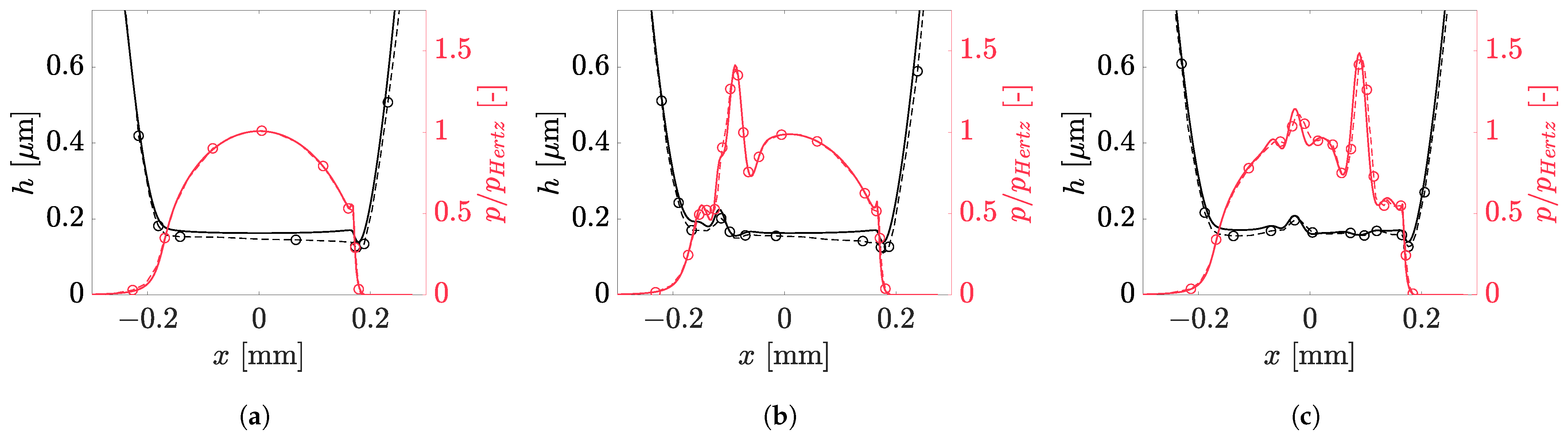
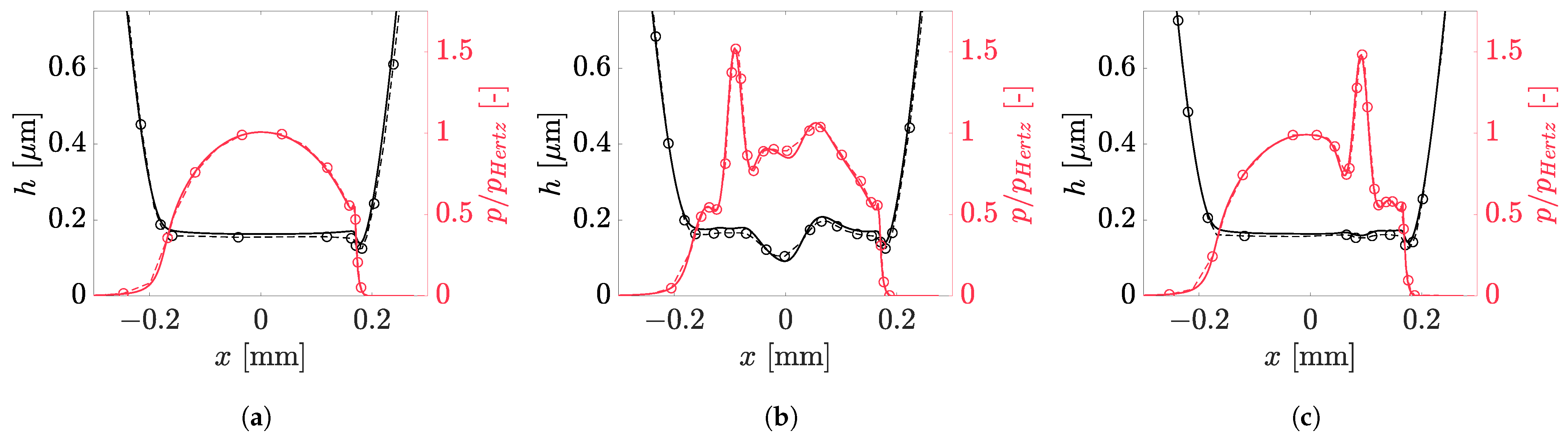
In Figure 2 and Figure 3, pressure and film thickness profiles at different simulation time values (hence different values of X d ) are presented for S R R = 1 (simple sliding, smooth surface moves faster than rough surface) and S R R = 2 (simple sliding, stationary smooth surface), respectively.
For both S R R values, the current model shows excellent agreement with the results in [7]. Quantitatively, for S R R = 1 , the root mean square error (RMSE) values for the normalised pressure distributions are in the range of 2.2 × 10 2 to 3.4 × 10 2 , while for the film thickness profiles the RMSE values are between 1.3 × 10 2 and 4.2 × 10 2 µm across the different time instances considered. Similarly, for S R R = 2 , the pressure RMSE values range from 1.9 × 10 2 to 7.5 × 10 2 , while the film thickness RMSE values range from 2.6 × 10 2 to 5.2 × 10 2 µm. It should be noted that the reference data used for the RMSE calculations were obtained by digitising the published figures in [7] using the PlotDigitizer Version 3.1.6 software [60], which operates on a pixel-based image grid with a snap-to-pixel functionality, resulting to the spatial resolution being limited by the pixel size of the image. With a digitisation error of ±0.5 pixel assumed, the resulting uncertainties for all validation figures are quantified in Appendix C. Overall, the digitisation uncertainties are an order of magnitude or more smaller than the RMSE values, confirming that the validation results are not affected by digitisation uncertainty. It should also be noted that certain numerical parameters required to exactly reproduce the results of Venner and Lubrecht are not explicitly specified in their paper. In particular, the convergence criterion of the EHL solver and the value of the pressure–viscosity coefficient exponent in the Roelands viscosity equation are not reported. In the present work, an EHL solver convergence criterion of 10 5 was used. Furthermore, a value of 0.6 was used for the pressure–viscosity coefficient exponent in the Roelands viscosity equation, consistent with the recommendation provided by Venner and Lubrecht in another study [10]. Despite the above, the low error magnitudes demonstrate that the present model is able to accurately reproduce the transient behaviours reported by Venner and Lubrecht.
In addition to the quantitative agreement, the model also reproduces the characteristic transient pressure and film thickness responses associated with moving surface features. According to Ai and Cheng [61], when the surface feature moves at a speed slower than the entrainment speed (Figure 2), the pressure ridge and surface indentation occur on the leading side and extend in front of the surface feature, whereas when the surface feature moves at a speed faster than the entrainment speed (Figure 3), a pressure ridge is formed at the trailing edge.
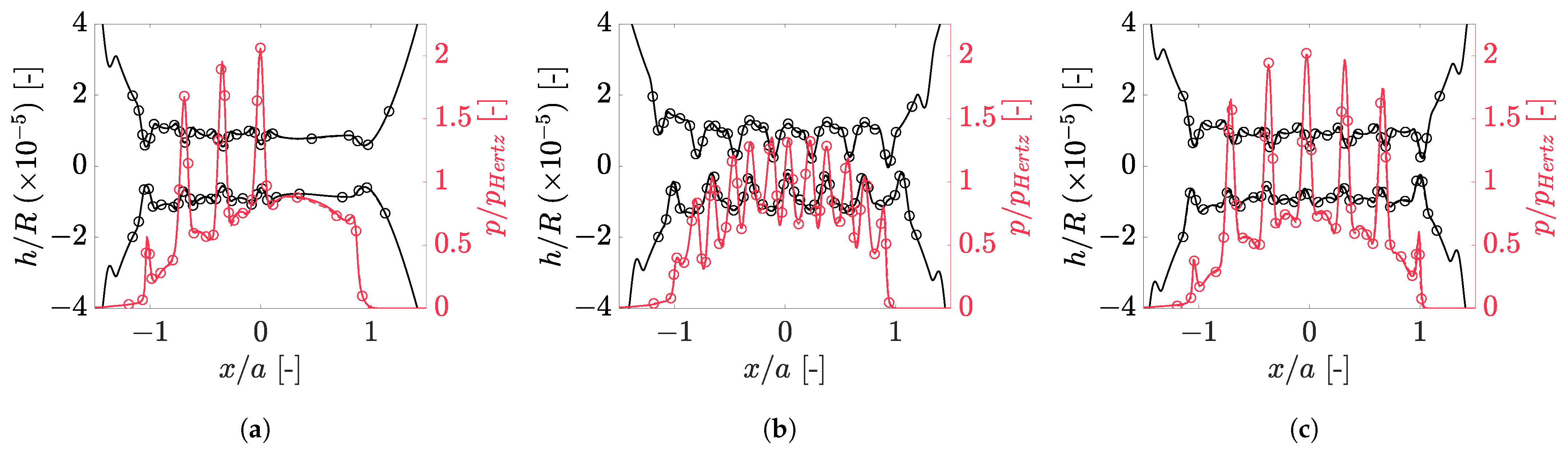
Further validation of the transient deterministic model was performed, comparing with the results of Cui et al. [20] who investigated the influence of two rough surfaces with transverse ridges moving against each other at different speeds. In contrast to the study by Venner and Lubrecht [7], Cui et al. [20] conducted all simulations under transient thermal conditions.
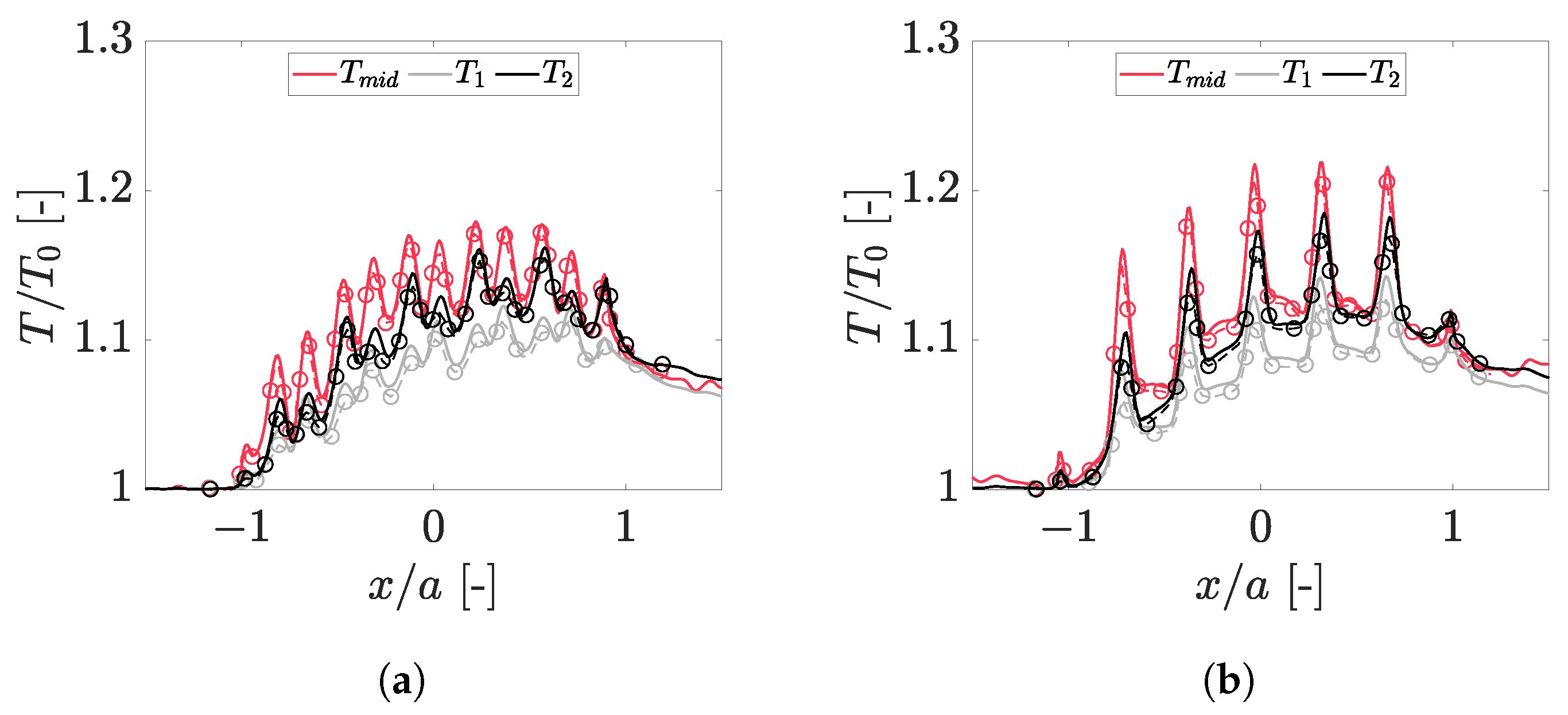
Figure 4 presents the evolution of centreline pressure and film thickness profiles at selected time iterations, while Figure 5 shows the corresponding mid-film and solid temperature distributions.
The agreement with the results of Cui et al. is excellent. Quantitatively, the RMSE values for the normalised pressure distributions are between 2.9 × 10 2 and 5.6 × 10 2 across the three considered time instances. Similarly, the dimensionless upper and lower surface film thickness profiles exhibit RMSE values of the order of 10 7 . These low error magnitudes demonstrate that the model accurately captures the transient interaction of surface features and the resulting hydrodynamic response.
Very good agreement is also observed for the temperature profiles in both the lubricant and solid domains. The dimensionless temperature RMSE values are of the order of 10 3 for the mid-film and solid temperatures at both considered time instances, confirming that the model accurately captures the overall shape and evolution of the temperature distributions, including the localised temperature rise associated with ridge interaction.
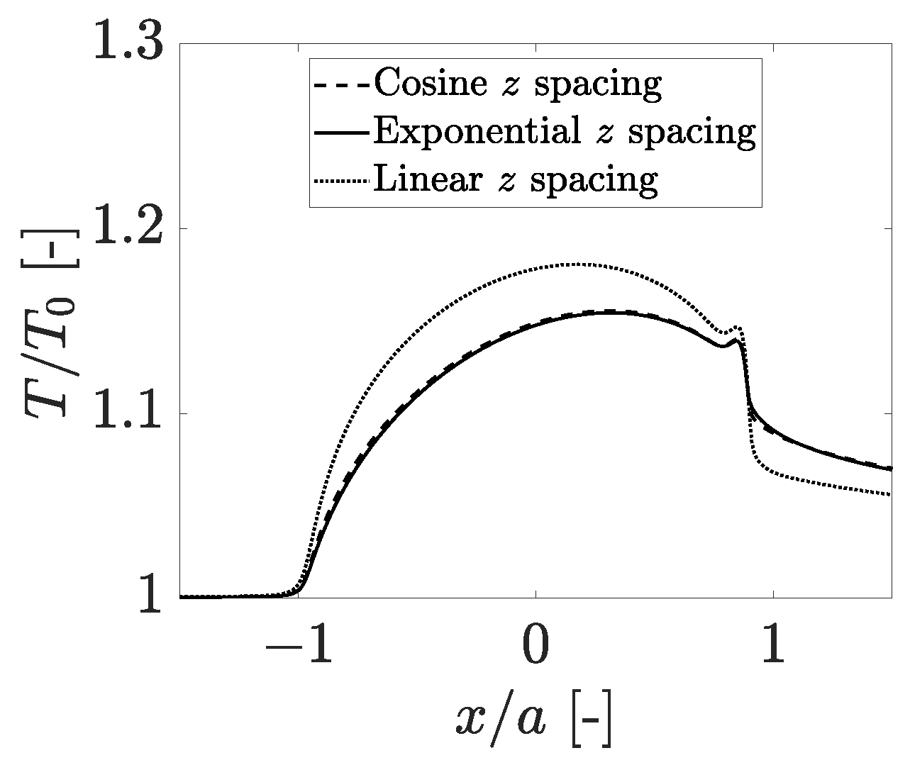
A slight deviation in the magnitude of the predicted temperatures can be attributed to the fact that the spacing of the nodes of the solid domain in the thickness (z) direction is not specified in [20]. In the present work, a non-uniform grid based on cosine spacing was employed to better resolve steep temperature gradients near the fluid–solid interface.
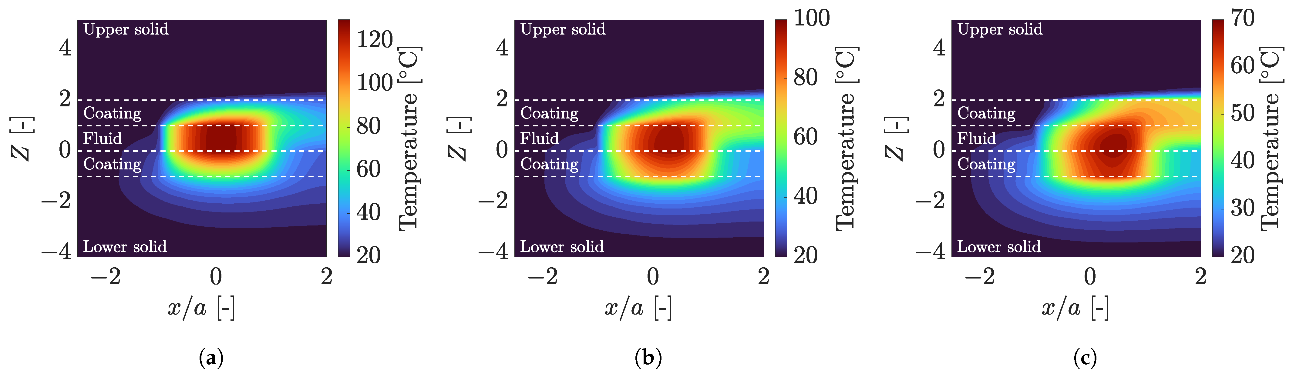
Additional simulations were carried out to assess the influence of the spacing of the nodes in the solids on the temperature field. As seen in Figure 6 these confirmed that the predicted temperature levels are sensitive to the node distribution in the solid, while the overall trends and spatial distributions remain unaffected.

3.1.2. Surface Coatings

To validate the accuracy of the surface coatings model, results were compared with those of Habchi [34] who investigated the influence of the mechanical and thermal properties of surface coatings on the pressure and film thickness profiles of a coated circular contact. To investigate the effect of the coatings’ mechanical properties, the authors independently varied the coatings’ thickness and Young modulus values. To investigate the effect of the coatings’ thermal properties, the authors varied the coatings’ thermal inertia (TI).
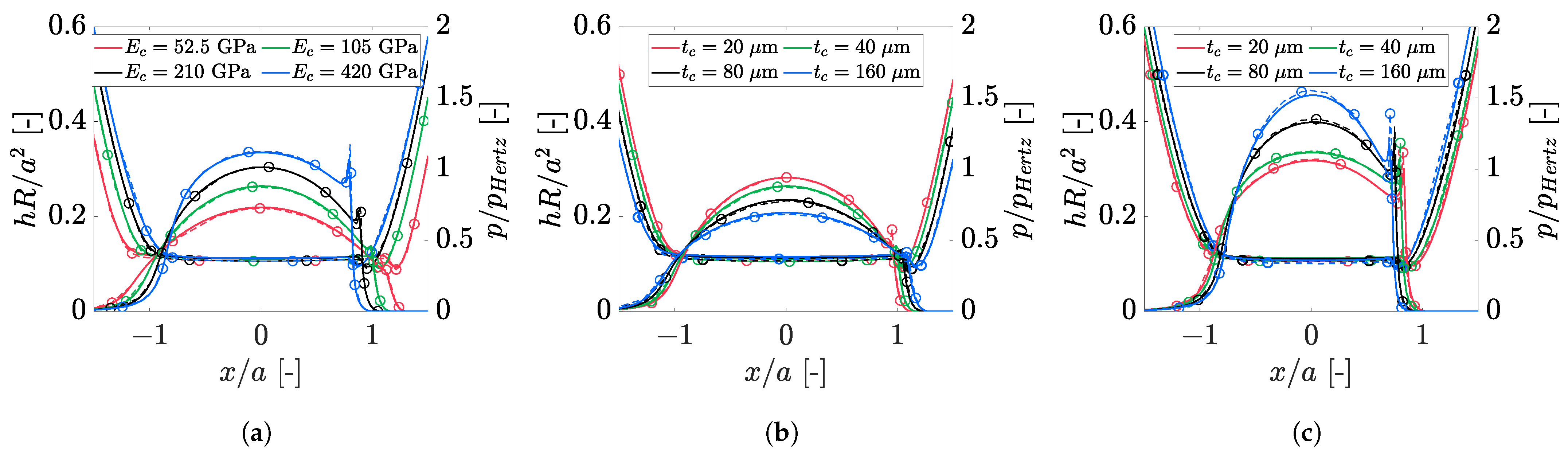
Figure 7 shows the effect of the coatings’ mechanical properties on the pressure and film thickness profiles. To study the effect of coating Young modulus, a coating thickness of 40 µm was used and to study the effect of coating thickness two different values for coating Young modulus were used: 105 GPa and 420 GPa.
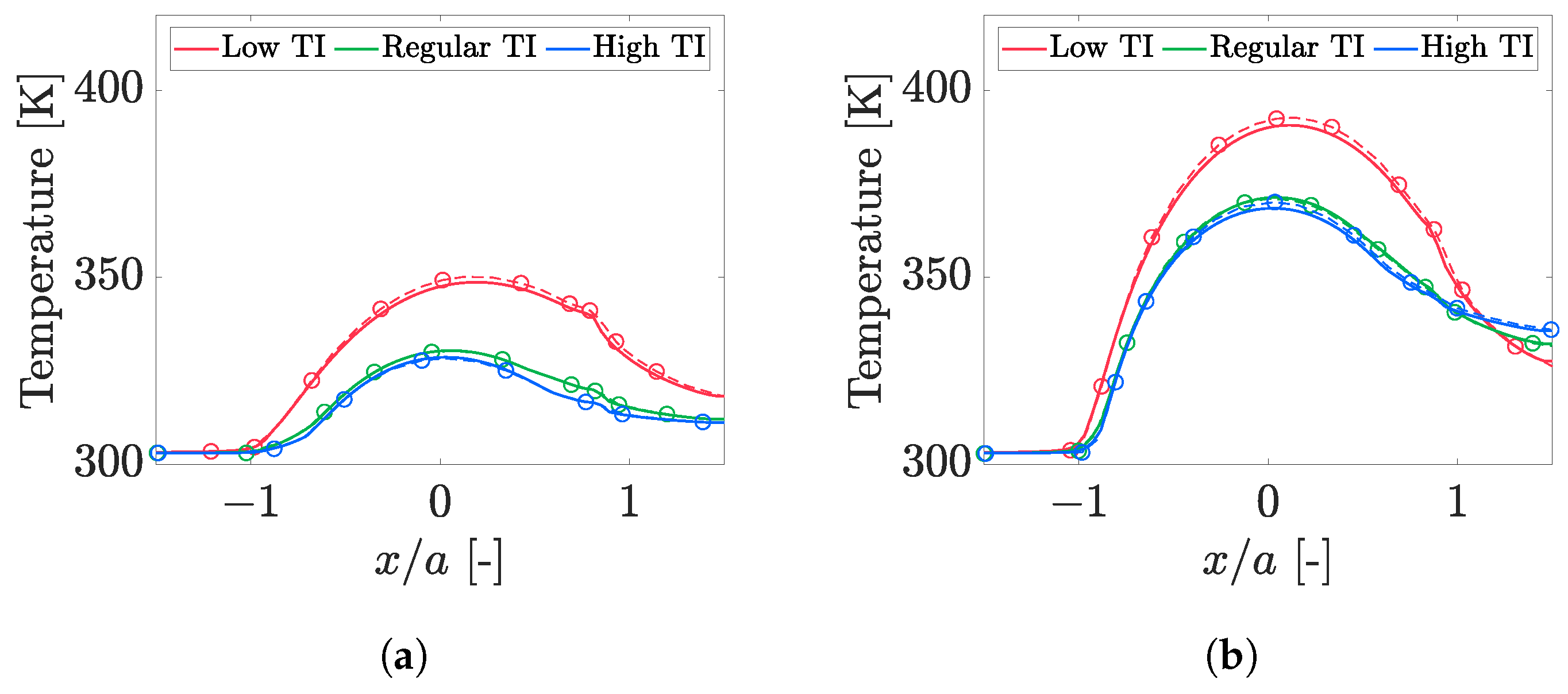
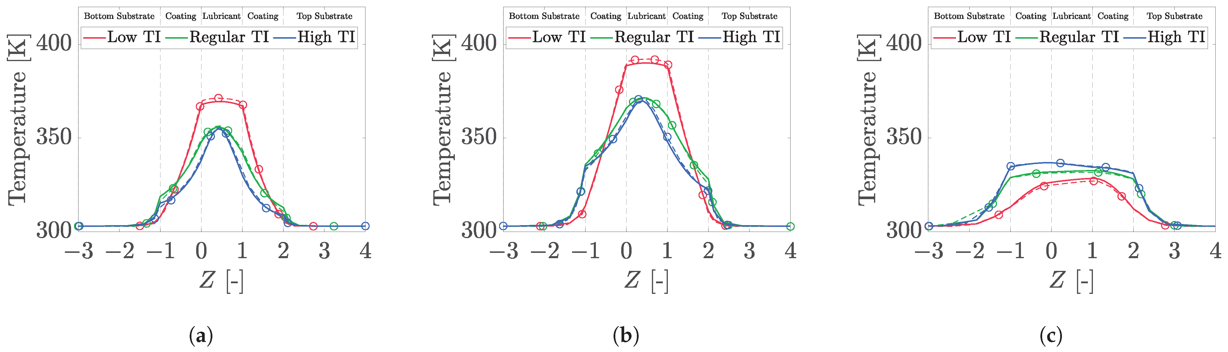
Figure 8 shows the effect of the coatings’ thermal properties, namely TI, on the mid-film temperature profiles at two different applied loads, 25 and 100 N. Figure 9 shows the effect of the coatings’ TI on the temperature profiles across the z-direction for an applied load of 100 N.
Overall, excellent agreement is also observed with the results of Habchi. The predicted pressure and film thickness profiles closely match the reference results for all considered coating configurations, accurately capturing the influence of both coating thickness and Young’s modulus on the contact behaviour, with RMSE values for the film thickness profiles of the order of 10 3 and RMSE values for the pressure profiles of the order of 10 2 . As reported by Habchi [34] and other studies like those of Liu et al. [33], increasing the coating Young’s modulus results in a higher maximum pressure and a smaller contact radius because the coating deforms less under the applied load. In contrast, softer coatings undergo greater elastic deformation, spreading the load over a larger contact area and reducing the peak pressure. Increasing the coating thickness amplifies these effects by reducing the influence of the substrate, allowing the coating properties to have a greater influence on the contact response. In contrast, the film thickness is only weakly affected by changes in coating Young’s modulus and thickness.
Similarly, very good agreement is obtained for the thermal results, with the maximum temperature RMSE value being 1.53 K occurring for the low-TI mid-film temperature profiles at an applied load of 100 N. The model successfully captures the influence of coating thermal inertia on the temperature distributions, including the variation in mid-film temperature and the distribution of temperature across the z-direction. The trends associated with both high and low thermal inertia coatings are well reproduced, confirming that the heat transfer within the coated system is accurately resolved.
Despite the use of a different numerical formulation (semi-system vs. Habchi’s full-system), the close agreement observed in both mechanical and thermal responses demonstrates the robustness and accuracy of the present approach for modelling coated EHL contacts.

3.2. Case Study 1

3.2.1. Effect of Mesh Size

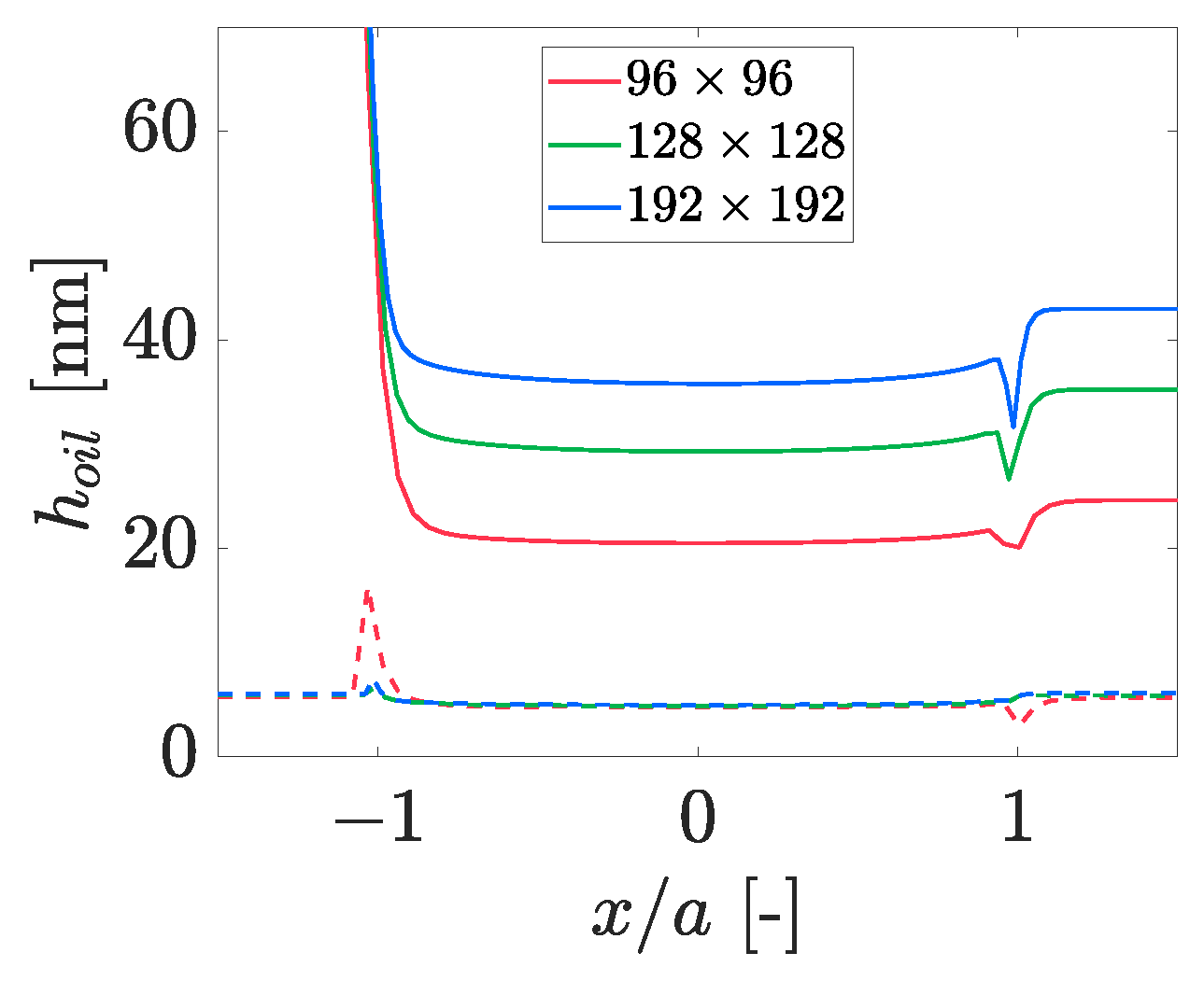
Figure 10 shows the centreline oil film thickness profiles for a smooth, isothermal case at both fully-flooded (solid lines) and starved (dashed lines) conditions for three different mesh sizes. For all three cases, the inlet oil film thickness was set to 6.25 nm, corresponding to the inlet oil film thickness for case study 1. As expected, the fully-flooded film thickness exhibits some dependence on mesh resolution, since the numerical solution of the Reynolds equation is influenced by the spatial discretisation. However, once the inlet oil film thickness is prescribed, the starved film thickness profiles show only negligible differences between the different mesh sizes. This demonstrates that the starved solution is governed primarily by the imposed inlet oil supply rather than the mesh resolution. Based on these results, the 128 × 128 mesh provides a satisfactory balance between numerical accuracy and computational cost and is therefore adopted for the remainder of this study.

3.2.2. Isotropic Sinusoidal Roughness

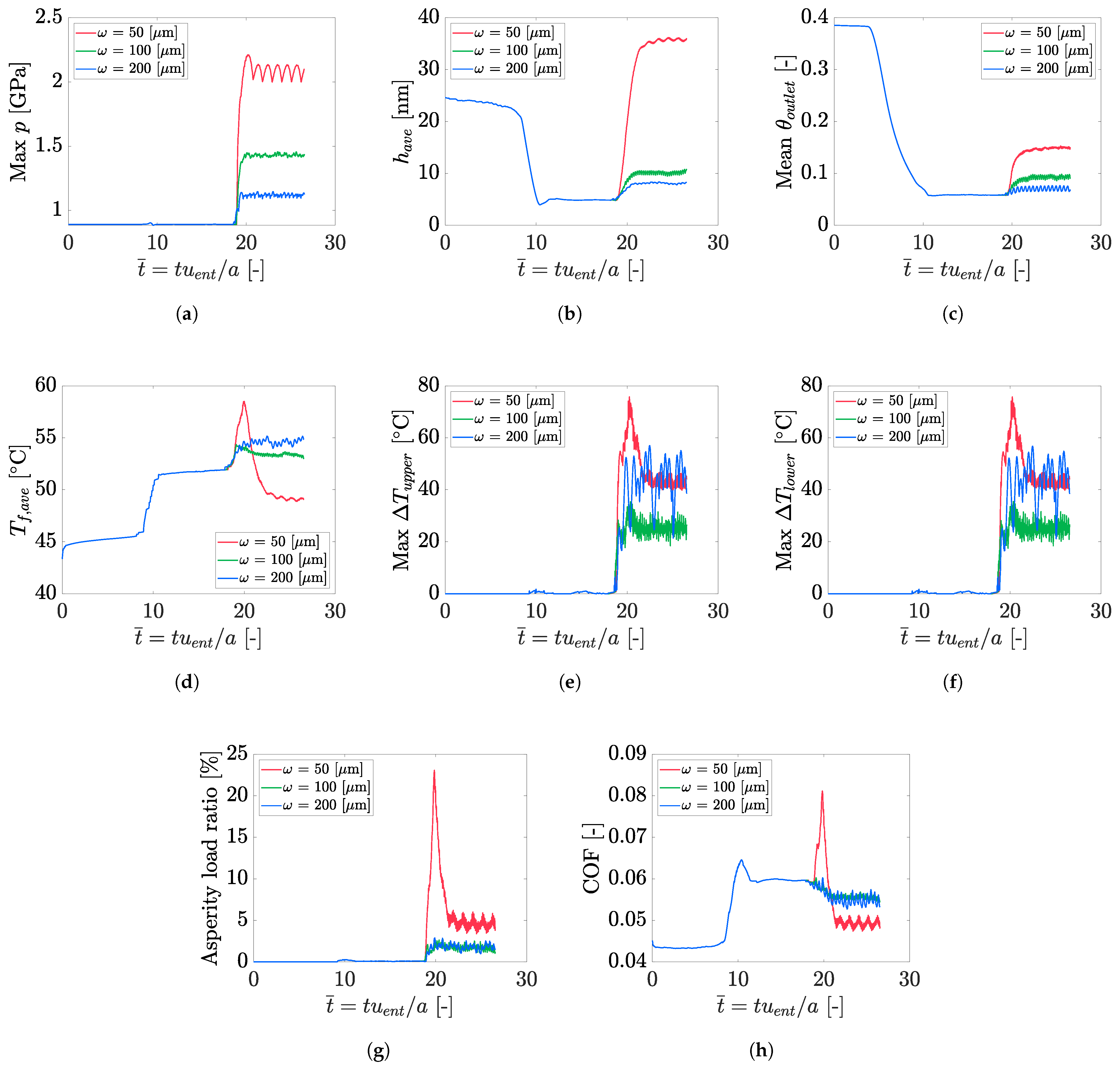
Figure 11 shows the evolution of key parameters with dimensionless time for the duration of the simulations as the starvation front and subsequently the isotropic sinusoidal roughness profiles move through the computational domain. In this case study, a variable time step ( Δ t ) was employed. For iterations N = 1 500 , a time step of Δ t = Δ x / u e n t was used, corresponding to a dimensionless Δ t ¯ = Δ X . For iterations N = 501 1000 , the time step is halved to Δ t = 0.5 · Δ x / u e n t or Δ t ¯ = 0.5 · Δ X to ensure the transient effects caused by the movement of the rough profiles are properly captured. In total, the simulation covers a dimensionless time, t ¯ , of 26.54. Iteration 1 represents a fully-flooded smooth case. From iteration 2 onwards, starvation was imposed at the inlet. Once the starvation front had moved through the contact and a steady state had been reached, a roughness profile started moving through the contact at N = 501 .
The maximum temperature rise values were calculated by subtracting the temperatures at asperity contact locations from the corresponding temperatures at those locations before the roughness profiles enter the contact, at a time when the system is at steady state. In this case, the reference temperatures were taken at t ¯ = 17.68 ( N = 500 ). The coefficient of friction (COF) presented is the average value of the COF calculated at the top and bottom surfaces. The z-coordinate in case study 1 was normalised in the following way:
  • Lower solid: Z = z 1 / a { 3.15 , 0 }
  • Fluid: Z = z / h { 0 , 1 }
  • Upper solid: Z = z 2 / a { 1 , 4.15 }
Figure 11 shows that the transient response of the system can be divided into four distinct phases.
Phase 1, covering t ¯ 0 10 , corresponds to the propagation of the starvation front from the inlet towards the Hertzian contact region. During this phase, the lubricant supply progressively decreases, leading to a reduction in film thickness as the inlet conditions begin to influence the contact. As the film becomes thinner, the shear rate within the lubricant increases, resulting in a gradual rise in the friction coefficient and fluid temperature. When the starvation front reaches the Hertzian zone, a sharp drop in film thickness is observed, accompanied by a sudden increase in temperature due to increased viscous heating. A brief occurrence of asperity contact may be observed at this point, but this is transient and the contact rapidly returns to full-film conditions.
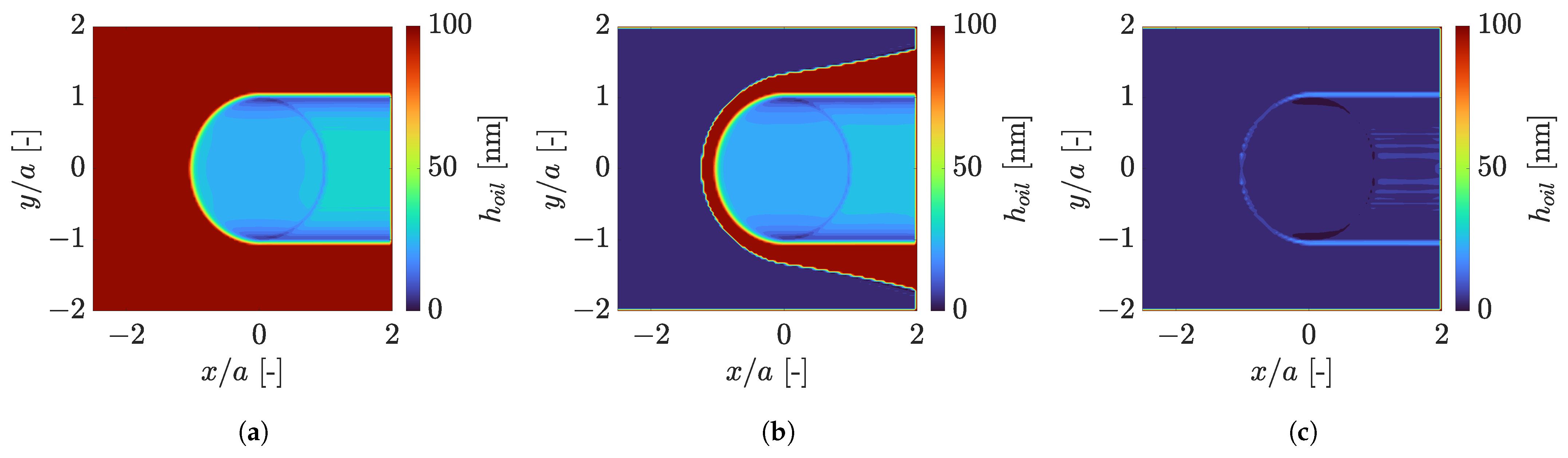
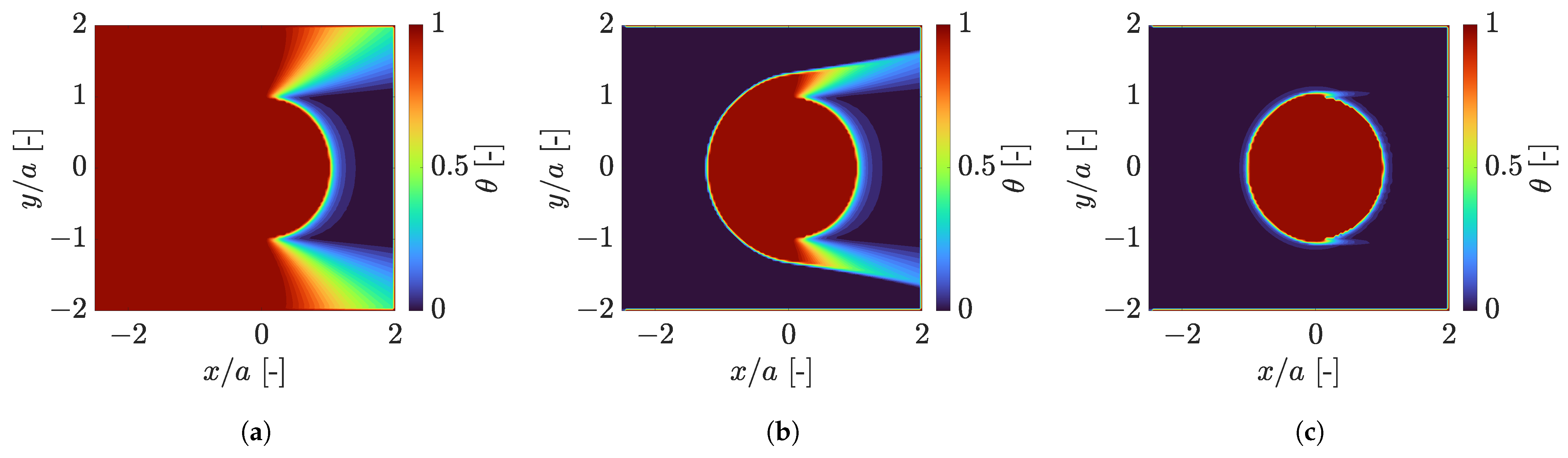
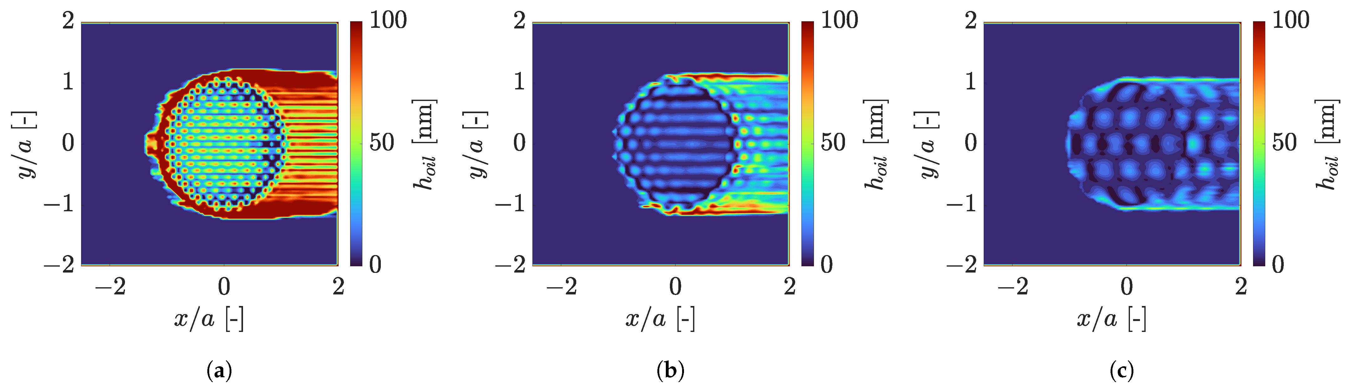
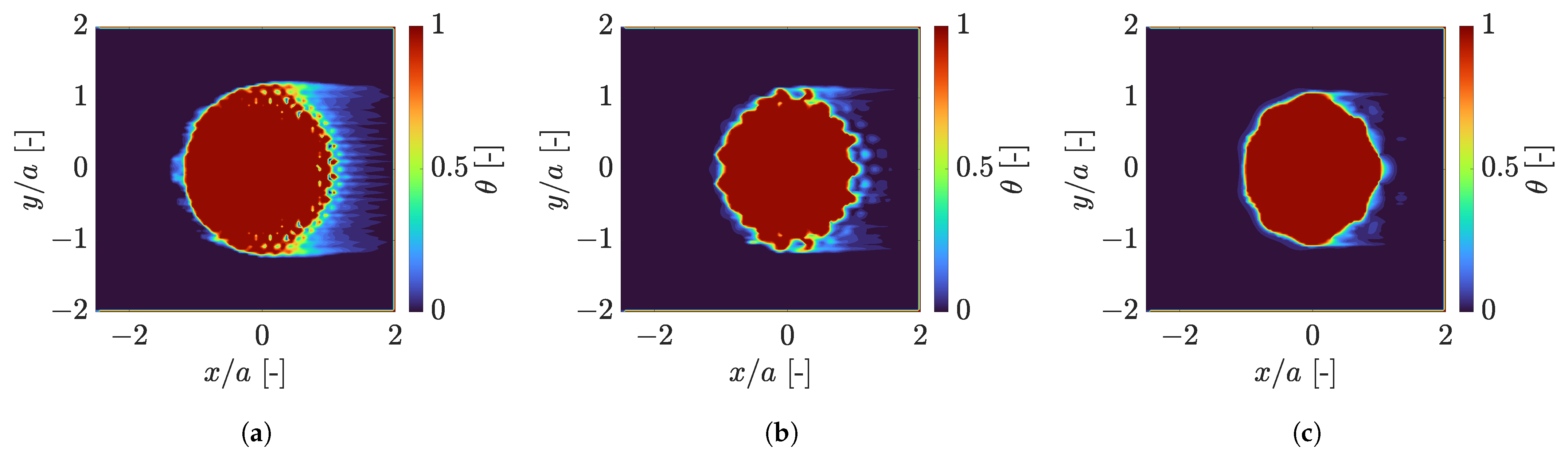
As seen in Figure 12 and Figure 13, which present contour plots of oil film thickness ( h o i l ) and liquid film fraction ( θ ), respectively, at different time iterations as the starvation front is moving through the contact, the starvation front moves faster at the edges of the contact than at the centre. The pressure is consistently higher along the centreline of the contact and decreases towards the edges. Hence, as the starvation front propagates and the lubricant supply is reduced, the pressure in the outer regions of the contact drops below the cavitation pressure earlier than at the centre. This leads to the onset of cavitation at the edges, with the central region remaining pressurised for longer, giving rise to the observed ’engulfing’ behaviour of the starvation front.
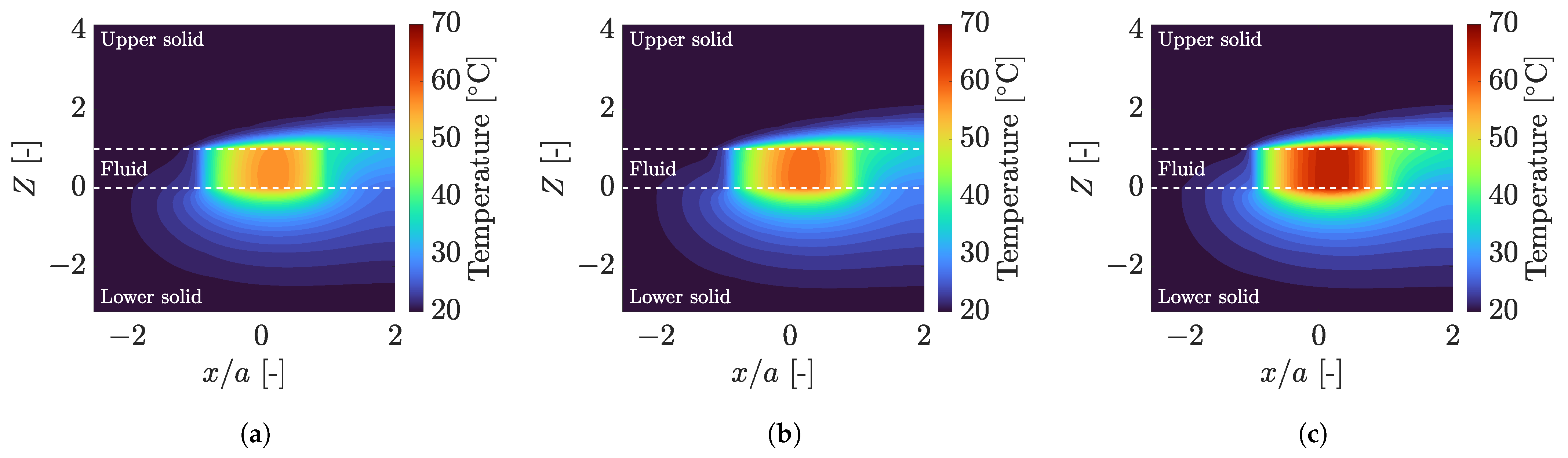
Phase 2, covering t ¯ 10 19 , corresponds to a starved steady state being reached for smooth solid surfaces. The film thickness stabilises at a reduced level governed by the inlet oil layer thickness and the friction coefficient correspondingly reaches a steady value. Figure 14 further illustrates the effect of starvation on the temperature distribution across the film thickness. As already mentioned, starvation leads to an overall increase in fluid temperature due to enhanced viscous heating under reduced film thickness. In addition, a noticeable change in the thermal profile across the film is observed. Under fully-flooded conditions, the temperature distribution is asymmetric, with higher temperatures near the stationary lower surface and lower temperatures near the moving upper surface. However, at starved conditions, the temperature distribution becomes significantly more uniform across the film thickness, with reduced thermal gradients between the two surfaces. This behaviour is primarily attributed to the reduced film thickness, which promotes a more uniform shear and heat generation within the lubricant layer.
Phase 3, covering t ¯ 19 22 , begins with the introduction of the deterministic roughness profiles into the starved contact. The roughness profiles enter the domain after t ¯ = 17.68 and propagate through the contact, reaching the centre of the Hertzian zone at t ¯ = 19.45 .
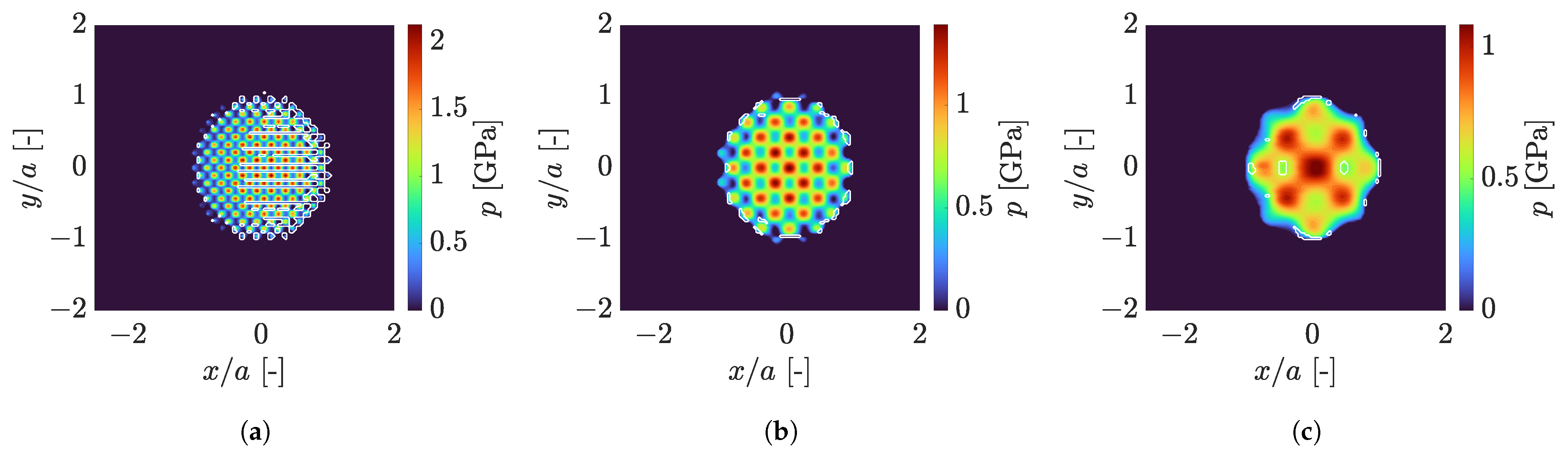
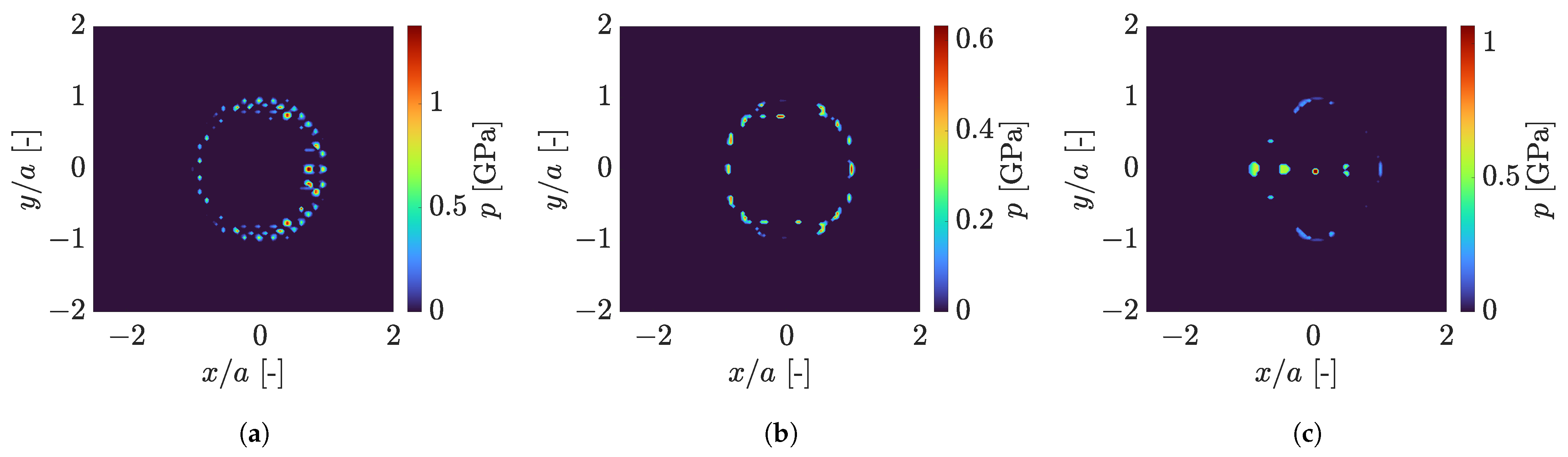
Across all wavelengths of isotropic sinusoidal profiles, the arrival of the roughness front induces local perturbations in film thickness, pressure and temperature, with the magnitude and nature of these perturbations strongly dependent on the wavelength. For the shortest wavelength ( ω = 50 µm), the roughness movement leads to pronounced asperity interactions, with the asperity load ratio exhibiting a sharp increase to approximately 23% before decreasing towards its steady-state value. Figure 15 shows the pressure profiles for the different roughness wavelengths at one time instance during Phase 3, with the white lines indicating regions of asperity contact.
Across all profiles, it is evident that asperity contacts primarily occur at low pressure regions. In particular, the shorter wavelength profiles produce deeper pressure troughs in the regions between asperity summits, corresponding to locations where the hydrodynamic load-carrying capacity is reduced. As a result, these regions are more prone to local film collapse and asperity interaction. The larger number of simultaneously occurring low-pressure regions within the Hertzian contact leads to a substantially higher transient asperity load ratio for the ω = 50 µm case. This effect is especially pronounced due to the already starved nature of the contact, where the lubricant film thickness is reduced and the surfaces are closer to interaction even before the roughness fronts enter the Hertzian zone.
For the shortest wavelength surface, the sharp transient increase in asperity load ratio is accompanied by significant fluctuations in friction and temperature with initial temperature peaks at asperity contact locations exceeding 75 °C above the baseline smooth case, indicating strong localised shear and asperity-scale heating. In contrast, for ω = 100 µm and ω = 200 µm, asperity interactions remain less pronounced, with only small transient increases in asperity load ratio of about 1.5–2.5% and temperature peaks of about 35 and 50 °C above the baseline, respectively.
The time it takes for the system to reach a steady state is also similar to results in the literature, with Wang and Zhu [45] reporting that it takes a dimensionless time of about t ¯ = 2 2.5 for a system with an evolving roughness profile to reach a stabilised solution, regardless of the time step chosen.
Phase 4 ( t ¯ 22 ) corresponds to a new steady state influenced by both starvation and surface topography. For the shortest wavelength ( ω = 50 µm), the system reaches a sustained asperity load ratio of approximately 3.5–5.5%. The coefficient of friction stabilises at approximately 0.047–0.051, which is significantly reduced compared to the value of the smooth starved case, despite the presence of asperity contacts. A similar behaviour has been observed in the studies of Cui et al. [20] and Kaneta et al. [22] where it was found that textured surfaces can result to lower coefficient of friction values compared to smooth surfaces, albeit their studies focused on fully-flooded cases with no asperity contacts.
For both the ω = 100 and 200 µm wavelengths, asperity load ratios at steady state are lower at about 1–2.5%. The coefficient of friction once again decreases to values below the smooth starved phase (0.053–0.055), which suggests that such wavelengths also enhance lubricant entrainment and promote film formation under starved conditions, but to a lesser degree compared to the shortest wavelength. The temperatures at the asperity locations exhibit oscillations between approximately 20 and 30 °C above the baseline for the ω = 100 µm wavelength and between approximately 25 and 50 °C above the baseline for the ω = 200 µm wavelength.
Further insight into the mechanisms underlying these behaviours is provided by the contour plots of oil film thickness and liquid film fraction distributions shown in Figure 16 and Figure 17. In the smooth starved case, the outlet region (defined as any point with x > 0 and not inside the Hertzian region) is characterised by a liquid film fraction close to zero, with a mean value of 0.06, indicating extensive cavitation. In contrast, the introduction of surface roughness leads to a noticeable increase in average film thickness and in liquid film fraction at the outlet, with the magnitude of this effect strongly dependent on the roughness wavelength. This behaviour is consistent with past studies like those of Venner and Lubrecht [62] which showed that additional lubricant can be dragged into the contact when waviness is introduced, especially when the rough surface is moving faster than the smooth one, as is the case in the present study. This enhanced entrainment helps to counteract the effects of starvation by promoting reformation of the lubricant film, which in turn reduces the coefficient of friction relative to the smooth starved case and contributes to the sustained, reduced asperity load ratio observed in Phase 4 relative to the initial transient overshoot in Phase 3.
For the shortest wavelength ( ω = 50 µm), this effect is particularly pronounced, with significant regions of non-zero liquid fraction observed throughout the outlet. The mean value of liquid film fraction at the outlet more than doubles compared to the smooth starved case to a value of 0.15. For the intermediate wavelength ( ω = 100 µm), the increase in liquid film fraction is also evident, although less pronounced, with the mean value of liquid film fraction at the outlet increasing to about 0.09. For the longest wavelength ( ω = 200 µm), the reformation of the lubricant film is the least pronounced, as the mean value of liquid film fraction at the outlet only increases to about 0.07. This is consistent with the relatively small changes in film thickness and friction, indicating that roughness-induced lubricant redistribution becomes less effective as the wavelength increases.
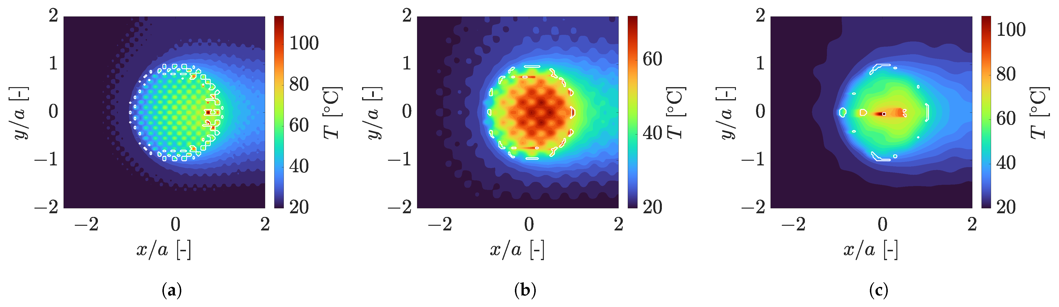
The mid-film temperature and asperity pressure distributions shown in Figure 18 and Figure 19, respectively, further highlight the strong influence of surface roughness on local thermal behaviour. For the shortest wavelength ( ω = 50 µm), pronounced localised hot spots are observed at asperity contact locations. These hot spots are consistent with the elevated asperity load ratio and increased friction observed for this case and indicate intense localised heat generation due to asperity interactions. As the roughness wavelength increases, asperity interactions become less frequent and the temperature field becomes smoother, with fewer localised perturbations associated with the passage of the roughness features. However, the magnitude of the maximum flash temperature rise does not decrease monotonically with increasing wavelength. In particular, the ω = 200 µm case exhibits larger local temperature peaks compared to the intermediate wavelength case, despite the lower pressure perturbations generated by the roughness features. Since the sliding velocity and boundary friction coefficient are identical for all cases, this difference is attributed primarily to the spatial distribution of the asperity contacts within the Hertzian region. For the longest wavelength profile, the asperity contacts occur closer to the centre of the Hertzian zone, where the resulting asperity pressure is higher. Consequently, although fewer asperities interact, the resulting local heat generation is higher. In contrast, for the intermediate wavelength ( ω = 100 µm) case, asperity interactions occur predominantly towards the outlet and side regions of the contact, where the resulting asperity pressures, limiting the maximum local temperature increase.
The average fluid temperature within the Hertzian region, excluding asperity contact locations, exhibits a different trend from the flash temperature response. As seen in Figure 11, the ω = 50 µm case results to the lowest average fluid temperature despite having the highest asperity load ratio, while increasing the roughness wavelength leads to higher average fluid temperatures. This behaviour is closely connected to lubricant replenishment phenomenon and the resulting average film thickness. As mentioned earlier, the shorter wavelengths exhibit a greater degree of lubricant reformation in the starved contact, leading to higher average film thickness values in the Hertzian zone, with 35 nm for ω = 50 µm, 10 nm for ω = 100 µm and 8 nm for ω = 200 µm. For a fixed entrainment and sliding speed, thicker films result to lower shear rates and therefore limit the viscous dissipation within the film. Although the shorter wavelength profiles also generate larger pressure variations, resulting in higher local viscosity peaks, the reduction in shear rate associated with the increased film thickness can have a dominant effect on the overall thermal response. Therefore, the ω = 50 µm case can result to lower average fluid temperatures despite the presence of higher local viscosity values. This is confirmed by integration of the viscous heating terms in the energy equations over the computational domain, which consistently results to lower total viscous heating values for smaller wavelengths.

3.2.3. Random Machined Roughness

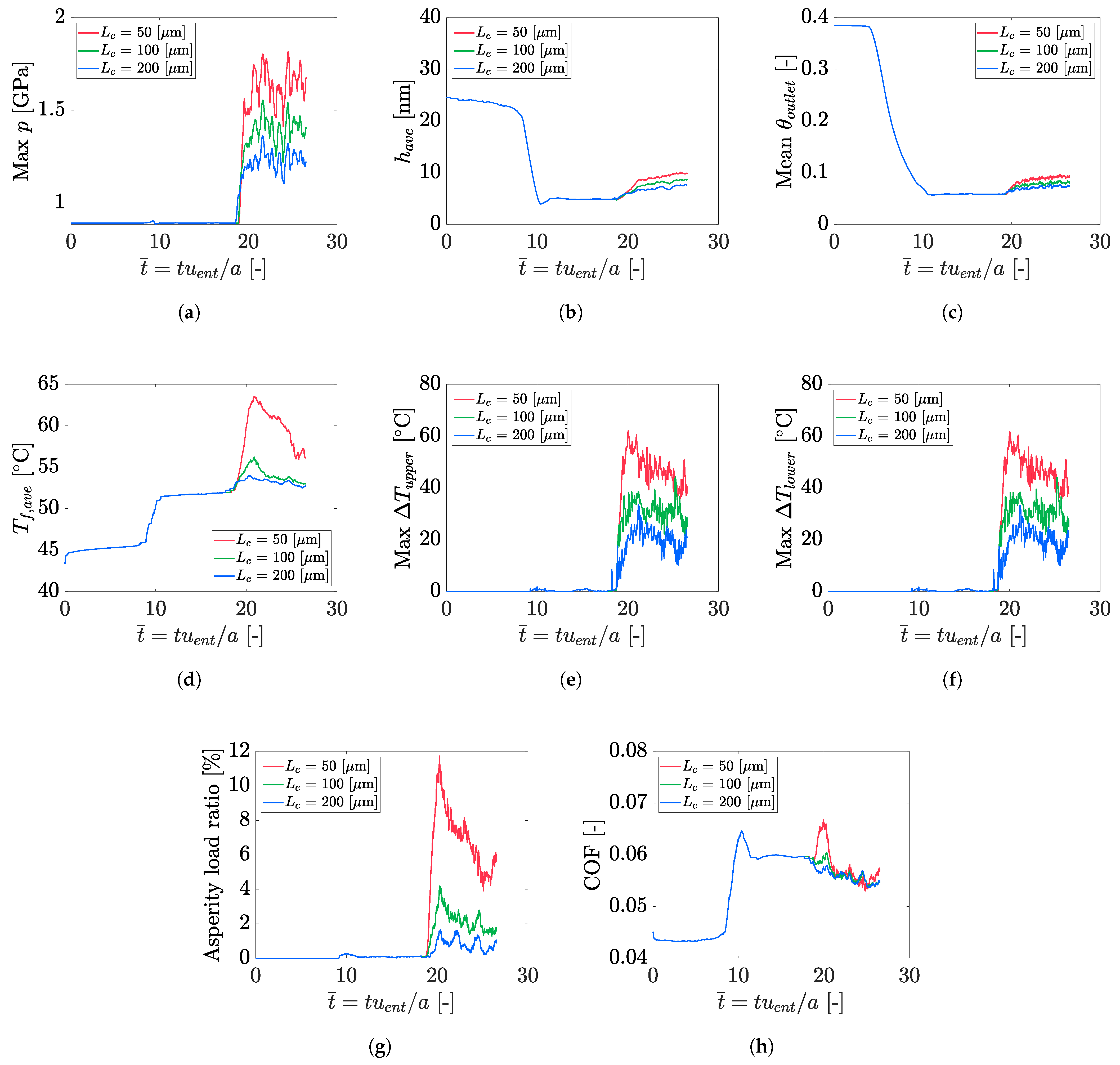
Figure 20 shows the evolution of key parameters with dimensionless time for the duration of the simulations as the starvation front and subsequently the random machined roughness profiles move through the computational domain.
Similar transient responses are observed compared to the periodic sinusoidal roughness profiles, but with a few differences in magnitude. For example, for the shortest correlation length ( L c = 50 µm), the asperity load ratio reaches a peak of about 12%, accompanied by a maximum temperature rise at asperity contact locations of about 60 °C above the baseline. These values are lower than the sinusoidal roughness transient peaks due to the fact that the random machined roughness profiles contain a distribution of asperity heights, with only some asperities reaching a peak amplitude of 0.1 µm while for the periodic profiles, all asperities reach that value. The shape of the transient evolution of the asperity load ratio is similar between the two types of roughness, indicating that the sharp increase is associated with the initial introduction of the roughness profiles into the previously smooth contact and is independent of any periodic effects. The asperity height distribution therefore influences the severity of the transient response rather than the mechanism by which it is generated.
With regard to the steady-state values, all correlation lengths result to a coefficient of friction that is smaller than the corresponding smooth starved case. The steady-state behaviour of the random machined surfaces appears to be less sensitive to the correlation length, compared to the dependence observed with the wavelength of the sinusoidal profiles. Reducing the correlation length increases the spatial density of asperity peaks within the Hertzian zone without producing the same systematic increase in local pressure observed for the periodic profiles, where every asperity reaches the full peak amplitude. This is reflected in the maximum local pressure, which increases only modestly as correlation length decreases, from 1.35 GPa ( L c = 200 µm) to 1.55 GPa ( L c = 100 µm) and 1.80 GPa ( L c = 50 µm), compared to the much larger increase observed for the equivalent sinusoidal wavelengths (up to 2.2 GPa). Also, the steady-state asperity load ratio shows only a modest increase with decreasing correlation length, from approximately 0.5% for L c = 200 µm, to 1.5% for L c = 100 and about 5% for L c = 50 µm. The increase in the mean values of liquid film fraction at the outlet as well as average film thickness at the Hertzian region also follow the same trend as the periodic profiles, with the shorter correlation length profiles leading to higher values, indicating a greater degree of lubricant replenishment. These are, however, less amplified compared to the periodic sinusoidal surface results.
Another interesting effect that is able to be captured by the proposed model is seen in Figure 21, which presents the temperature distributions at the lower fluid–solid interface. In addition to the expected localised hot spots at asperity contact locations (indicated by the white lines), a trailing ’hot track’ is observed immediately behind each contact, extending in the direction of surface motion. This behaviour reflects transient heat transfer phenomena associated with the passage of the roughness profiles, whereby heat generated at contact locations gradually dissipates within the solids, producing an elongated thermal wake rather than a stationary hot spot. This is consistent with experimental observations of flash temperatures in sliding contacts, where asperity contacts result to streaks of elevated temperatures behind them [63].
For the machined roughness profiles, this thermal wake effect could also contribute to the observed differences in average fluid temperature between correlation lengths. The shorter correlation length surfaces generate a greater number of asperity interactions, resulting in a larger number of overlapping thermal wakes within the Hertzian region. Although the total viscous heating contribution across the domain once again decreases with decreasing correlation length, the average lubricant temperature is higher overall for shorter correlation lengths. This indicates that the lubricant temperature is influenced not only by the instantaneous heat generation, but also by the accumulated thermal history associated with repeated asperity interactions and the resulting thermal wakes.
Capturing this effect relies directly on the transient, fully-coupled solution of the energy equation in both the lubricant and solid domains. Because the asperity-scale temperature field is resolved directly through the energy equations, the model is able to track the evolving thermal history of the fluid and solids. A steady-state formulation would be unable to reproduce this effect, since it depends explicitly on the time history of the roughness passage rather than on the instantaneous local contact conditions alone. This highlights the importance of a fully-transient, directly resolved thermal formulation for capturing the transient thermal response of rough, starved EHL contacts.
Overall, the results of case study 1 demonstrate that surface roughness can have a significant influence on the evolution and steady-state behaviour of starved EHL contacts. For the deterministic sinusoidal profiles, the roughness wavelength controls the balance between lubricant replenishment and asperity interactions. Shorter wavelengths promote stronger lubricant reformation, leading to increased film thickness, reduced average fluid temperatures and lower friction compared to the smooth starved case, although this occurs alongside increased asperity interactions and higher local flash temperatures. In contrast, longer wavelengths reduce asperity interactions but provide a less effective enhancement of the lubricant film. Therefore, the influence of surface roughness is inherently non-monotonic, with the optimal surface characteristics depending on the competing effects of enhanced lubricant entrainment and increased localised asperity interactions.
The random machined roughness results further demonstrate that these mechanisms are not restricted to idealised periodic surfaces. Although the magnitude of the transient response is reduced due to the distribution of asperity heights, the same fundamental behaviour is observed, with roughness-induced lubricant reformation leading to reduced friction compared to the smooth starved contact. Furthermore, the transient thermal results highlight the importance of resolving the coupled, time-dependent interaction between roughness passage, asperity heating and heat transfer within the solid domains. The ability of the present framework to capture local flash temperature peaks and thermal wakes provides additional insight into the mechanisms governing the thermal response of realistic rough, starved EHL contacts.

3.3. Case Study 2

Figure 22 shows the evolution of key parameters with dimensionless time for the duration of the simulations as the starvation front moves through the computational domain. In total, the simulation consisted of 500 time iterations, with a uniform time step of Δ t = Δ x / u e n t , covering a dimensionless time, t ¯ , of 17.68. As was the case in case study 1, iteration 1 was a fully-flooded smooth case. From iteration 2 onwards, starvation was imposed at the inlet. The z-coordinate in case study 2 was normalised in the following way:
  • Lower solid: Z = z 1 / a { 4.15 , 1 }
  • Lower coating: Z = z c 1 / h c 1 { 1 , 0 }
  • Fluid: Z = z / h { 0 , 1 }
  • Upper coating: Z = z c 2 / h c 2 { 1 , 2 }
  • Upper solid: Z = z 2 / a { 2 , 5.15 }
Under fully-flooded conditions, clear differences are already observed between the coating configurations. As seen in Figure 23a, the maximum fluid temperature is highest for the low-TI coatings (approximately 105 °C), followed by the regular-TI coatings (approximately 85 °C) and the high-TI coatings (approximately 68 °C). This trend reflects the ability of the coatings to dissipate heat, with low-TI coatings acting as thermal barriers, limiting heat conduction into the solids, while high-TI coatings promote efficient heat removal from the contact. The COF follows the opposite trend, with values of approximately 0.013, 0.027 and 0.043 for low, regular and high-TI coatings, respectively. This behaviour is attributed to the strong temperature-viscosity coupling of the lubricant with higher fluid temperatures in the low-TI case reducing the effective viscosity, thereby lowering shear stress and friction. This is consistent with previous numerical and experimental studies [64,65,66,67] attributing the change in friction to the effect of temperature on viscosity. It should be noted, however, that an alternative explanation proposed in the literature attributes part of the friction reduction observed with certain coatings to interfacial slip between the lubricant and the coated surface, rather than to thermal effects alone. As the present model does not include a slip boundary condition, it is not able to capture this mechanism, and the friction reduction predicted here only reflects the contribution of the thermal effects. This represents a limitation of the current model and a direction for future work.
When starvation is imposed, these trends become more pronounced. The reduction in lubricant supply leads to thinner films and increased shear, resulting in higher temperatures across all cases. The maximum fluid temperature rises to approximately 130 °C for the system with low-TI coatings, compared to approximately 95 °C for the system with regular-TI coatings and a seemingly negligible rise for the system with high-TI coatings. This indicates that the influence of thermal inertia becomes increasingly important under starved conditions, where heat generation is intensified and efficient heat dissipation is critical. It is interesting to note that the film thickness evolution across all three systems with different coatings is very similar even though the temperature and resulting viscosity are different. That is because film thickness in the Hertzian zone is governed by the conditions at the low pressure inlet region [68]. The pressure, temperature, viscosity and density profiles in that region are almost identical between the three different systems both under fully-flooded and starved conditions. In contrast, friction is primarily influenced by the high pressure central region, which is significantly different across the different systems.
The evolution of the COF under starvation further highlights the interplay between thermal and hydrodynamic effects. The COF increases for all cases due to the reduction in film thickness and subsequent increase in shear stress. However, the magnitude of this increase depends strongly on the coating properties. The most significant increase is observed for the high-TI coating (from approximately 0.043 to 0.065), while the regular-TI case increases more moderately (from approximately 0.027 to 0.039). In contrast, the low-TI coating exhibits only a small increase in COF (from approximately 0.013 to 0.018). This again reflects the importance of temperature-related reduction in viscosity, which almost offsets the increase in shear rate, hence COF, due to starvation.
The temperature distributions across the z-direction provide further insight into the role of coating thermal inertia on heat partitioning within the contact. As shown in Figure 23a and Figure 24, noticeable differences are observed in the thermal gradients across the lubricant film prior to starvation. The system with high-TI coatings exhibits larger temperature gradients across the film thickness, whereas the system with low-TI coatings shows a more uniform temperature distribution, with the regular-TI coatings system exhibiting an intermediate behaviour. Since the shear rates remain comparable across the different systems, these differences in gradients are not primarily associated with variations in viscous heat generation. Furthermore, the convective heat transport remains of similar magnitude across all cases. However, for the low-TI coating, the ratio of convection through the fluid to conduction into the solids is higher, implying that a larger fraction of the generated thermal energy remains confined within the lubricant film, promoting a more uniform fluid temperature distribution across the film thickness. In contrast, the more pronounced heat conduction into the solids with high-TI coatings results in steeper temperature gradients across the film thickness.
After starvation is imposed (Figure 23c and Figure 25), the thermal gradients across the film are significantly reduced in all cases, resulting in a more uniform temperature distribution across the lubricant film. This flattening if primarily attributed to the reduction in film thickness under starvation. As the film thickness decreases, the shear rate distribution becomes more uniform across the film thickness, resulting to a more uniform viscous heat generation. This behaviour is largely independent of the coating properties. This is supported by the fact that the relative differences in temperature gradients between the different coating configurations are preserved, with the low-TI coating system leading to the flattest temperature distribution across the film and the high-TI coating leading to the least uniform. This indicates that heat partitioning at the coating interfaces, which is governed by the thermal properties of the coatings, continues to determine the differences between systems, while the overall flattening is governed by the reduction in film thickness itself.
Overall, the results demonstrate that coating thermal inertia plays a critical role in controlling both temperature rise and frictional behaviour in starved contacts. Coatings with low thermal inertia lead to higher temperatures but lower friction due to viscosity reduction, whereas coatings with high thermal inertia limit fluid temperature rise but result in higher friction. The effect of starvation amplifies these differences, highlighting the importance of considering both thermal transport and transient operating conditions when evaluating coating performance.

4. Conclusions

In this work, a unified transient deterministic lubrication model was developed within a finite volume framework on a curvilinear grid. The model extends previous full-film TEHL formulations to a unified treatment of boundary, mixed and full-film lubrication regimes through the implementation of a semi-system approach. In contrast to many existing mixed lubrication studies, thermal effects within the solids are resolved directly through the solution of the energy equation, enabling the transient evolution of temperature fields within both the lubricant and solid domains to be captured without reliance on analytical flash temperature approximations. Furthermore, the framework incorporates transient starvation, deterministic surface roughness and coating behaviour within a single unified formulation.
Two case studies were used to rigorously demonstrate the predictive capability and physical fidelity of the proposed framework. The first case study on transient starvation reveals that the system response is not continuous but organised into distinct, resolvable phases, governed by the propagation of the starvation front through the contact. Starvation induces a systematic collapse of film thickness, which in turn drives sharp increases in friction and temperature through enhanced viscous shear. Crucially, the model resolves the spatio-temporal evolution of cavitation, showing accelerated front propagation along contact edges where local pressures are lower; an effect that is typically not captured with reduced-order approaches.
Introducing deterministic roughness under starved conditions showcases the ability of textured surfaces to affect the behaviour of starved systems by promoting lubricant replenishment and counteracting the negative effects of starvation. Such effect is particularly evident with shorter wavelength periodic rough surfaces, although such shorter wavelengths can also result to increased asperity interactions and higher local flash temperatures. The results show that such behaviours are also evident in real, non-periodic engineering surfaces. These results demonstrate that surface topography is not intrinsically detrimental under starvation, but can instead be strategically tuned to enhance performance.
The second case study establishes coating thermal properties as a first-order control parameter governing coupled thermal-tribological behaviour under transient starvation. Low thermal inertia coatings lead to high lubricant temperatures due to poor heat dissipation, yet simultaneously produce lower friction via viscosity reduction. Conversely, high thermal inertia coatings suppress temperature rise but incur friction penalties due to elevated viscosity. Starvation amplifies this trade-off, highlighting that coating performance cannot be assessed under steady-state assumptions alone, and must instead be evaluated within a transient, coupled thermofluid framework.
Beyond these specific findings, the framework captures fully-coupled transient heat transport across lubricant, coating, and substrate domains, resolving both through-thickness thermal gradients and the propagation of asperity-induced hot spots into the solids. This represents a clear advance over conventional flash temperature models, which cannot access such multi-domain, time-resolved behaviour.
Overall, the proposed framework establishes a step change in the modelling of transient lubrication, providing a unified, conservative, and physically grounded treatment that seamlessly bridges full-film, mixed, and boundary regimes under realistic operating conditions. By explicitly resolving the coupled dynamics of flow, roughness, starvation, and heat transport, it moves beyond descriptive analysis towards predictive, mechanism-aware simulation of tribological systems. Crucially, this capability enables the exploration of design spaces that were previously inaccessible, including the co-optimisation of surface topography and coating properties under transient, non-equilibrium conditions. Looking forward, the framework provides a natural foundation for integration with data-driven and AI-enhanced methodologies, supporting accelerated materials discovery, real-time performance prediction, and adaptive control strategies. In this context, it underpins an emerging paradigm in which tribological systems are no longer empirically tuned, but instead digitally designed, interrogated, and optimised through physics-informed virtual environments.

Author Contributions

Conceptualisation, F.K., S.A., D.D. and J.P.E.; Methodology, F.K. and S.A.; Software, F.K. and S.A.; Validation, F.K. and S.A.; Formal Analysis, F.K.; Investigation, F.K.; Resources, D.D. and J.P.E.; Data Curation, F.K.; Writing—Original Draft Preparation, F.K. and S.A.; Writing—Review and Editing, D.D. and J.P.E.; Visualisation, F.K.; Supervision, D.D. and J.P.E.; Project Administration, D.D.; Funding Acquisition, D.D. and J.P.E. All authors have read and agreed to the published version of the manuscript.

Funding

EPSRC UK iCASE studentship (EP/X524773/1), EPSRC UK InFUSE Prosperity Partnership (EP/V038044/1).

Data Availability Statement

Raw data used to plot the figures can be found online at: https://doi.org/10.5281/zenodo.20486910.

Acknowledgments

D.D. acknowledges the support of the Royal Academy of Engineering (RAEng) for the Shell/RAEng Research Chair in Complex Engineering Interfaces. J.P.E. acknowledges the support of the RAEng through their Research Fellowships scheme.

Conflicts of Interest

The authors declare that they have no known competing financial interests or personal relationships that could have appeared to influence the work reported in this paper.

Appendix A. Nomenclature

Table A1. List of symbols.
SymbolParameter
ARoughness amplitude
A ¯ Dimensionless roughness amplitude
aHertzian contact radius
cLubricant specific heat capacity
c i Specific heat capacity of solid body i
c j Specific heat capacity of coating layer j
D u 3 Continuous influence coefficient for normal surface displacement
D ^ ^ u 3 Discrete influence coefficient for normal surface displacement
D s Thickness of solid body s
E Reduced elastic modulus of elasticity
E 1 , E 2 Young’s modulus of lower and upper solids, respectively
E j Young’s modulus of coating layer j
e p , θ Pressure-film fraction convergence criterion
e g l o b a l p Global pressure convergence criterion
e T Temperature convergence criterion
e g l o b a l T Global temperature convergence criterion
e W Load convergence criterion
f b Boundary friction coefficient
G j Shear modulus of coating layer j
G u 3 Frequency response function of the normal surface displacement
hGeometric film thickness
h c , f f Central film thickness under fully-flooded conditions
h j Thickness of coating layer j
h o i l Lubricant film thickness
h 0 Rigid body separation
kLubricant thermal conductivity
k i Thermal conductivity of solid body i
k j Thermal conductivity of coating layer j
LTotal number of coating layers in each solid
NTime iteration
N x , N y , N z Number of discretisation points along each coordinate direction
pPressure
p ^ ^ Fourier-transformed pressure distribution
p a Asperity contact pressure
p c a v Cavitation pressure
R x , R y Equivalent radii of curvature along the x- and y-directions, respectively
R q Root mean square roughness
r p , θ Pressure-film fraction residual
r g l o b a l p Global pressure residual
r T Temperature residual
r g l o b a l T Global temperature residual
r W Load residual
s 1 , s 2 Time-dependent surface roughness profiles of lower and upper solids, respectively
S R R Slide-to-roll ratio
TFluid temperature
T 0 Reference (ambient) temperature
T i Temperature of solid body i
tTime
t ¯ Dimensionless time
u , v , w Fluid velocities in the x-, y- and z-directions, respectively
u i , v i , w i Velocities of solid body i in x-, y- and z-directions, respectively
u e n t Entrainment speed in the x-direction
u s Sliding speed in the x-direction
u 3 Normal elastic deformation
u 3 ( j ) Fourier-transformed normal displacement in coating layer j
WApplied load
X d Dimensionless position of roughness profile in the domain
x d Position of roughness profile in the domain
x s Position of roughness profile in the domain at t = 0
Y Shape function
ZNormalised fluid domain coordinate
Z i Normalised solid domain coordinate
Z j Normalised coating domain coordinate
α Distance of a node ( m , n ) to the origin in the frequency domain
α p Pressure–viscosity coefficient
β Coefficient of fluid thermal expansion
γ ˙ Shear rate
γ m e s h         Mesh refinement coefficient
δ Normal elastic deformation
η Fluid viscosity
η 0 Reference fluid viscosity
θ Liquid film fraction
μ Friction coefficient
ν 1 , ν 2 Poisson’s ratio of lower and upper solids, respectively
ν j Poisson’s ratio of coating layer j
ρ Fluid density
ρ c Density of the saturated fluid at cavitation conditions
ρ i Density of solid body i
ρ j Density of coating layer j
ρ 0 Reference fluid density
τ Hydrodynamic shear stress
τ a Asperity contact shear stress
τ E Eyring shear stress
Ω Computational domain
ω Periodic roughness wavelength
ω ¯ Dimensionless periodic roughness wavelength

Appendix B. Finite Volume Discretisation

Appendix B.1. Discretisation of the Generalised Reynolds Equation

The finite volume discretisation of the dimensionless mass-conserving ( p θ ) generalised Reynolds equation within the semi-system lubrication framework yields the following linearised algebraic equation for each control volume:
α ( p ¯ W ) + β ( p ¯ P ) + γ ( p ¯ E ) + ζ ( p ¯ N ) + λ ( p ¯ S ) = φ ,
where the nodal pressures associated with the west, centre, east, north, and south neighbouring control volumes are defined as follows:
p ¯ W = p ¯ i 1 , j , p ¯ P = p ¯ i , j , p ¯ E = p ¯ i + 1 , j ,
p ¯ N = p ¯ i , j + 1 , p ¯ S = p ¯ i , j 1 .
The coefficients α , β , γ , ζ , and the source term φ arise from the discretisation of the diffusive, convective, and transient contributions of the governing equation. In the following expressions, the subscripts ‘D’, ‘C’, and ‘t’ denote the diffusive, convective, and transient contributions, respectively. The lowercase directional subscripts w, e, n, and s indicate quantities evaluated at the corresponding control volume faces using arithmetic interpolation, whereby:
( ε ¯ ) w = ( ε ¯ ) W + ( ε ¯ ) P 2 .
The entrainment-flow and transient terms are discretised using a second-order upwind scheme in order to improve the numerical stability and accuracy under strongly convective and transient operating conditions.
α D = ( ε ¯ ) w · ( Δ Y ) w / ( Δ X ) w α C = ( Δ Y ) w · [ 2 · ( ρ ¯ e * U m + ρ ¯ 1 * U 1 ) i 1 · θ i 1 · D k , l i , j + 0.5 · ( ρ ¯ e * U m + ρ ¯ 1 * U 1 ) i 2 · θ i 2 · D k 1 , l i 2 , j ] α t = ( Δ Y ) w · 1.5 · ρ ¯ e · θ i · D k 1 , l i , j / Δ t ¯ α = α D + α C + α t
β D = ( ε ¯ ) w · ( Δ Y ) w / ( Δ X ) w ( ε ¯ ) e · ( Δ Y ) e / ( Δ X ) e r x y 2 ( ε ¯ ) n · ( Δ X ) n / ( Δ Y ) n r x y 2 ( ε ¯ ) s · ( Δ X ) s / ( Δ Y ) s β C = ( Δ Y ) w · 1.5 · ( ρ ¯ e * U m + ρ ¯ 1 * U 1 ) i · θ i · D k , l i , j + 0.5 · ( ρ ¯ e * U m + ρ ¯ 1 * U 1 ) i 2 · θ i 2 · D k , l i 2 , j β t = ( Δ Y ) w · 1.5 · ρ ¯ e · θ i · D k , l i , j / Δ t ¯ β = β D + β C + β t
γ D = ( ε ¯ ) e · ( Δ Y ) e / ( Δ X ) e γ C = ( Δ Y ) e · 1.5 · ( ρ ¯ e * U m + ρ ¯ 1 * U 1 ) i · θ i · D k + 1 , l i , j + 0.5 · ( ρ ¯ e * U m + ρ ¯ 1 * U 1 ) i 2 · θ i 2 · D k + 1 , l i 2 , j γ t = ( Δ Y ) e · 1.5 · ρ ¯ e · θ i · D k + 1 , l i , j / Δ t ¯ γ = γ D + γ C + γ t
ζ D = 0 ζ C = 0 ζ t = 0 ζ = ζ D + ζ C + ζ t
λ D = 0 λ C = 0 λ t = 0 λ = λ D + λ C + λ t
φ D = ( p ¯ ) N · r x y 2 ( ε ¯ ) n · ( Δ X ) n / ( Δ Y ) n + ( p ¯ ) S · r x y 2 ( ε ¯ ) s · ( Δ X ) s / ( Δ Y ) s φ C = 1.5 · ( ρ ¯ e * U m + ρ ¯ 1 * U 1 ) i · θ i · H i D k , l i , j · p ¯ k , l + D k + 1 , l i , j · p ¯ k + 1 , l 2 · ( ρ ¯ e * U m + ρ ¯ 1 * U 1 ) i 1 · θ i 1 · H i 1 D k 1 , l i 1 , j · p ¯ k 1 , l + 0.5 · ( ρ ¯ e * U m + ρ ¯ 1 * U 1 ) i 2 · θ i 2 · H i 2 D k 1 , l i 2 , j · p ¯ k 2 , l + D k , l i 2 , j · p ¯ k , l + D k + 1 , l i 2 , j · p ¯ k + 1 , l φ t = { 1.5 · ρ ¯ e · θ i · H i D k 1 , l i , j · p ¯ k 1 , l + D k , l i , j · p ¯ k , l + D k + 1 , l i , j · p ¯ k + 1 , l 2 · ρ ¯ e N 1 · θ i N 1 · H i N 1 + 0.5 · ρ ¯ e N 2 · θ i N 2 · H i N 2 } / Δ t ¯ φ = φ D + φ C + φ t
Table A2. Normalised variables and discretisation parameters used in the finite volume formulation of the semi-system generalised Reynolds equation.
SymbolParameterDefinition
D k , l i , j Influence coefficient relating the pressure at node ( k , l ) to the elastic deformation at node ( i , j )
HNormalised film thickness h / a
p ¯ Normalised pressure p / p Hertz
NTime level
r x y Grid aspect ratio Δ x / Δ y
U 1 , U 2 Normalised velocities of the lower and upper surfaces in the sliding direction u 1 / u ent , u 2 / u ent
U m Normalised mean entrainment velocity ( U 1 + U 2 ) / 2
Δ t ¯ Normalised time step Δ t u ent / a
Δ X , Δ Y Normalised control volume face dimensions in the x- and y-directions Δ x / a , Δ y / a
( Δ X ) w , e Normalised distances between neighbouring nodes in the west and east directions
( Δ Y ) n , s Normalised distances between neighbouring nodes in the north and south directions
( Δ Y ) w , e , ( Δ X ) n , s Normalised face lengths associated with west/east and north/south control volume faces
ε ¯ Normalised pressure-flow coefficient in the generalised Reynolds equation ε η 0 / ( ρ 0 a 3 )
ρ ¯ e Normalised equivalent density integrated across the film thickness ρ e / ( ρ 0 a )
ρ ¯ e * Normalised entrainment-flow density coefficient ρ e * / ρ 0
ρ ¯ 1 * Normalised surface-velocity density coefficient ρ 1 * / ρ 0
θ Lubricant film fraction 0 θ 1
α , β , γ , ζ , λ Algebraic coefficients associated with west, central, east, north, and south pressure nodes
φ Source term of the discretised Reynolds equation

Appendix B.2. Discretisation of the Fluid Energy Equation

The dimensionless energy equation governing thermal transport within the lubricant film is presented below for a general non-orthogonal curvilinear coordinate system, following the formulation proposed by Ardah et al. [44]:
Pe ( H ρ ¯ c ¯ T ¯ ) t ¯ + Pe X · ( ρ ¯ c ¯ V ˜ T ¯ ) = X · κ ˜ ¯ X T ¯ + Q ˜ ¯ p + Q ˜ ¯ c + Q ˜ ¯ Φ + q ˙ ˜ ¯ V .
The dimensionless variables and source terms are defined as follows:
H = h a , ρ ¯ = ρ ρ 0 , c ¯ = c c 0 , T ¯ = T T 0 , η ¯ = η η 0 , β ¯ = β β 0 , ϵ = h c a , p ¯ = p ϵ 2 a η 0 u e n t .
The normalised source-term contributions associated with compressive heating/cooling ( Q ˜ ¯ p ), enthalpic effects ( Q ˜ ¯ c ), viscous dissipation ( Q ˜ ¯ Φ ), and volumetric heat generation ( q ˙ ˜ ¯ V ) are expressed as follows
Q ˜ ¯ p = Br * β ¯ T ¯ H p ¯ t ¯ + V ˜ X p ¯ X + V ˜ Y p ¯ Y ,
Q ˜ ¯ c = Pe ρ ¯ T ¯ H c ¯ t ¯ + V ˜ · X c ¯ ,
Q ˜ ¯ Φ = Br η ¯ H 3 V ˜ X Z 2 + 1 r x y V ˜ Y Z 2 ,
q ˙ ˜ ¯ V = H q ˙ ˜ V .
The governing dimensionless groups appearing in the thermal formulation are given as follows:
Pe = ρ 0 c 0 u e n t a ϵ 2 k 0 , Br = η 0 u e n t 2 k 0 T 0 , Br * = β 0 T 0 Br ,
where Pe is the Peclet number, Br is the Brinkman number, and Br * is the modified Brinkman number.
The finite volume discretisation of the dimensionless energy equation is obtained by combining the spatial discretisation procedure proposed by Ardah et al. [44] with a first-order backward temporal discretisation following the approach outlined by Moukalled in [36]. The resulting discretised formulation is presented below.
Pe ( Δ V C V ) P H ρ ¯ c ¯ T ¯ P N H ρ ¯ c ¯ T ¯ P N 1 Δ t ¯ + α ( T ¯ W ) + β ( T ¯ P ) + γ ( T ¯ E ) + ζ ( T ¯ N ) + λ ( T ¯ S ) + ϕ ( T ¯ T ) + ψ ( T ¯ B ) = φ .
The neighbouring temperature values appearing in Equation (A9) correspond to west, central, east, north, south, top, and bottom nodes of the control volume and are defined as follows:
T ¯ W = T ¯ i 1 , j , k , T ¯ P = T ¯ i , j , k , T ¯ E = T ¯ i + 1 , j , k , T ¯ N = T ¯ i , j + 1 , k , T ¯ S = T ¯ i , j 1 , k , T ¯ T = T ¯ i , j , k + 1 , T ¯ B = T ¯ i , j , k 1 .
The coefficients α , β , γ , ζ , λ , ϕ , ψ and φ are defined below. In these expression, the subscripts ‘D’ and ‘C’ refer to the the diffusive and convective contributions arising from the diffusive and convective terms of the energy equation, respectively.
α D = ( ϵ ) 2 · k ¯ w · H w · S w / ( Δ X ) w α C = ρ ¯ c ¯ V ˜ X w · Pe · S w , 0 α = α D + α C
γ D = ( ϵ ) 2 · k ¯ e · H e · S e / ( Δ X ) e γ C = ρ ¯ c ¯ V ˜ X e · Pe · S e , 0 γ = γ D + γ C
ζ D = ( r x y ϵ ) 2 · k ¯ n · H n · S n / ( Δ Y ) n ζ C = ρ ¯ c ¯ V ˜ Y n · Pe · S n , 0 ζ = ζ D + ζ C
λ D = ( r x y ϵ ) 2 · k ¯ s · H s · S s / ( Δ Y ) s λ C = ρ ¯ c ¯ V ˜ Y s · Pe · S s , 0 λ = λ D + λ C
ϕ D = ( k ¯ t · S t ) · [ 1 + ϵ 2 · X · H t 2 · Z t 2 + ϵ r x y 2 · Y · H t 2 · Z t 2 ] / H · ( Δ Z ) t ϕ C = ρ ¯ c ¯ V ˜ Z t · Pe · S t , 0 ϕ = ϕ D + ϕ C
ψ D = ( k ¯ b · S b ) · [ 1 + ϵ 2 · X · H b 2 · Z b 2 + ϵ r x y 2 · Y · H b 2 · Z b 2 ] / H · ( Δ Z ) b ψ C = ρ ¯ c ¯ V ˜ Z b · Pe · S b , 0 ψ = ψ D + ψ C
β D = α D γ D ζ D λ D ϕ D ψ D β C = ρ ¯ c ¯ V ˜ X e · Pe · S e , 0 + ρ ¯ c ¯ V ˜ Y n · Pe · S n , 0 + ρ ¯ c ¯ V ˜ Z t · Pe · S t , 0 + ρ ¯ c ¯ V ˜ X w · Pe · S w , 0 + ρ ¯ c ¯ V ˜ Y s · Pe · S s , 0 + ρ ¯ c ¯ V ˜ Z b · Pe · S b , 0 β = β D + β C
φ = Q ˜ ¯ p P + Q ˜ ¯ c P + Q ˜ ¯ Φ P + ( q ˙ ˜ ¯ V ) P · ( Δ V C V ) P
The operator A , B denotes the maximum between A and B. The lowercase subscripts w, e, n, s, t, and b indicate the quantities evaluated at the corresponding control volume faces using arithmetic averaging. For example,
( c ¯ ) w = ( c ¯ ) W + ( c ¯ ) P 2 .
Table A3. Normalised variables and discretisation parameters used in the finite volume formulation of the lubricant energy equation.
SymbolParameterDefinition
c ¯ Normalised specific heat capacity c / c 0
HNormalised lubricant film thickness h / a
κ ˜ ¯ Dimensionless diffusion tensor in the transformed coordinate system
p ¯ Normalised pressure p ϵ 2 a / ( η 0 u ent )
S Outward surface vector normal to a control-volume face
T ¯ Normalised temperature T / T 0
V ˜ Dimensionless contravariant velocity vector in the transformed domain V ˜ X , V ˜ Y , V ˜ Z T
V ˜ X , V ˜ Y , V ˜ Z Dimensionless contravariant velocity components in the X-, Y-, and Z-directions
X , Y , Z Normalised coordinates in the sliding, transverse, and film-thickness directions x / a , y / a , z / h
β ¯ Normalised coefficient of thermal expansion β / β 0
Δ X , Δ Y , Δ Z Normalised control-volume dimensions in the transformed coordinate directions
Δ V C V Control-volume volume in the transformed domain ( Δ X ) ( Δ Y ) ( Δ Z )
ϵ Film-thickness-to-contact-length scale ratio h c / a
η ¯ Normalised dynamic viscosity η / η 0
ρ ¯ Normalised density ρ / ρ 0
Pe Peclet number ρ 0 c 0 u ent a ϵ 2 / k 0
Br Brinkman number η 0 u ent 2 / ( k 0 T 0 )
Br * Modified Brinkman number β 0 T 0 Br

Appendix B.3. Discretisation of Heat Transport in Solid and Coated Domains

The finite volume discretisation of the energy equation within the coating and substrate domains follows the same procedure as that used for the lubricant energy equation presented in Appendix B.2. The principal distinction is that no volumetric heat-generation source terms are included within the solid regions, since heat generation is assumed to arise predominantly from viscous dissipation within the lubricant film and frictional heating at asperity contact locations. Consequently, thermal transport in the solid domains is governed primarily by transient heat conduction and convective transport associated with the motion of the bounding surfaces. The in-plane discretisation in the x- and y-directions remains fully consistent with that employed for the lubricant domain, thereby preserving spatial compatibility across the coupled fluid–solid system. In contrast, the out-of-plane discretisation in the z-direction is defined according to the physical thickness of each coating layer and substrate region. This enables the thermal response of thin coatings, multilayered interfaces, and bulk substrates to be resolved accurately within the coupled thermo-hydrodynamic formulation.
To accurately capture the thermal gradients that develop near the interfaces, local mesh refinement is introduced in the vicinity of the fluid-coating and coating-substrate interfaces. In particular, increased mesh resolution in the z-direction ensures accurate evaluation of the interfacial heat fluxes and temperature gradients governing thermal continuity across neighbouring domains.The thermal coupling between neighbouring domains is enforced through the heat-flux continuity conditions given by Equations (19) and (20). Equation (19) ensures continuity of conductive heat flux across fluid–solid interfaces, while Equation (20) governs heat transfer across asperity contact regions by accounting for frictionally generated heat at solid–solid junctions, hence ensuring thermodynamic consistency throughout the coupled conjugate heat-transfer problem.

Appendix C. Validation Figures Digitisation Uncertainties

The uncertainties in x and y resulting from the digitisation process of the validation figures and presented in Table A4 are calculated in the following way, with an error equal to ±0.5 pixels:
Δ x = x - range x - resolution · 0.5 , Δ y = y - range y - resolution · 0.5
Table A4. Digitisation process uncertainties.
FigureImage ResolutionVariableAxis RangeEstimated Uncertainty
Figure 2 and Figure 3824 × 676x [mm]−0.4 to 0.4 [mm] 4.9 × 10 4 [mm]
Figure 2 and Figure 3824 × 676 p / p H e r t z [-]0 to 2 [-] 1.5 × 10 3 [-]
Figure 2 and Figure 3824 × 676h [µm]0 to 1 [µm] 7.4 × 10 4 [µm]
Figure 4 and Figure 5961 × 688 x / a [-]−1.2 to 1.2 [-] 1.2 × 10 3 [-]
Figure 4961 × 688 p / p H e r t z [-]0 to 2.5 [-] 1.8 × 10 3 [-]
Figure 4961 × 688 h / R [-] 2 × 10 5 to 2 × 10 5 [-] 2.9 × 10 8 [-]
Figure 5961 × 688 T / T 0 [-]1 to 1.25 [-] 1.8 × 10 4 [-]
Figure 71254 × 934 x / a [-]−2 to 1.5 [-] 1.4 × 10 3 [-]
Figure 71254 × 934 p / p H e r t z [-]0 to 2 [-] 1.1 × 10 3 [-]
Figure 71254 × 934 h R / a 2 [-]0 to 0.6 [-] 3.2 × 10 4 [-]
Figure 81254 × 934 x / a [-]−1.5 to 1.5 [-] 1.2 × 10 3 [-]
Figure 8 and Figure 91254 × 934Temperature [K]300 to 420 [K] 6.4 × 10 2 [K]
Figure 91254 × 934Z [-]−3 to 4 [-] 3.7 × 10 3 [-]

References

  1. Lugt, P.M.; Morales-Espejel, G.E. A review of elasto-hydrodynamic lubrication theory. Tribol. Trans. 2011, 54, 470–496. [Google Scholar] [CrossRef] [Scilit]
  2. Ardah, S.; Profito, F.J.; Dini, D. A comprehensive review and trends in lubrication modelling. Adv. Colloid Interface Sci. 2025, 342, 103492. [Google Scholar] [CrossRef] [Scilit] [PubMed]
  3. Morales-Espejel, G.E.; Wemekamp, A.W. Ertel-Grubin method in elastohydrodynamic lubrication—A review. Proc. Inst. Mech. Eng. Part J 2008, 222, 15–34. [Google Scholar] [CrossRef] [Scilit]
  4. Lubrecht, A.A.; Napel, W.E.T.; Bosma, R. The influence of longitudinal and transverse roughness on the elastohydrodynamic lubrication of circular contacts. J. Tribol. 1988, 110, 421–426. [Google Scholar] [CrossRef] [Scilit]
  5. Patir, N.; Cheng, H.S. An Average Flow Model for Determining Effects of Three-Dimensional Roughness on Partial Hydrodynamic Lubrication. J. Lubr. Technol. 1978, 100, 12–17. [Google Scholar] [CrossRef] [Scilit]
  6. Patir, N.; Cheng, H.S. Application of Average Flow Model to Lubrication Between Rough Sliding Surfaces. J. Lubr. Technol. 1979, 101, 220–229. [Google Scholar] [CrossRef] [Scilit]
  7. Venner, C.H.; Lubrecht, A.A. Numerical Simulation of a Transverse Ridge in a Circular EHL Contact Under Rolling/Sliding. J. Tribol. 1994, 116, 751–761. [Google Scholar] [CrossRef] [Scilit]
  8. Zhu, D.; Hu, Y.Z. The Study of Transition from Elastohydrodynamic to Mixed and Boundary Lubrication. In Proceedings of the Advancing Frontier of Engineering Tribology: Proceedings of the 1999 STLE/SAME H.S. Cheng Tribology Surveillance, Golden, CO, USA, 11–13 October 1999. [Google Scholar]
  9. Hu, Y.; Zhu, D. A Full Numerical Solution to the Mixed Lubrication in Point Contacts. J. Tribol. 2000, 122, 1–9. [Google Scholar] [CrossRef] [Scilit]
  10. Venner, C.H.; Lubrecht, A.A. Multilevel Methods in Lubrication; Tribology Series; Elsevier: Amsterdam, The Netherlands, 2000; Volume 37, pp. 57–100. [Google Scholar]
  11. Liu, S.; Wang, Q.; Liu, G. A versatile method of discrete convolution and FFT (DC-FFT) for contact analyses. Wear 2000, 243, 101–111. [Google Scholar] [CrossRef] [Scilit]
  12. Zhu, D. On some aspects of numerical solutions of thin-film and mixed elastohydrodynamic lubrication. Proc. Inst. Mech. Eng. Part J 2007, 221, 561–579. [Google Scholar] [CrossRef] [Scilit]
  13. Pu, W.; Wang, J.; Zhu, D. Progressive Mesh Densification Method for Numerical Solution of Mixed Elastohydrodynamic Lubrication. J. Tribol. 2016, 138, 021502. [Google Scholar] [CrossRef] [Scilit]
  14. Blok, H.A. Theoretical study of temperature rise at surfaces of actual contact under oiliness lubricating conditions. Proc. Instn. Mech. Engrs. 1937, 2, 222–235. [Google Scholar]
  15. Jaeger, J.C. Moving sources of heat and the temperature at sliding contacts. J. Proc. R. Soc. N. S. W. 1942, 76, 203–224. [Google Scholar] [CrossRef] [Scilit]
  16. Carslaw, H.S.; Jaeger, J.C. Conduction of Heat in Solids; Oxford University Press: London, UK, 1959. [Google Scholar]
  17. Zhu, D.; Wang, J.; Wang, Q.J. On the Stribeck Curves for Lubricated Counterformal Contacts of Rough Surfaces. J. Tribol. 2015, 137, 021501. [Google Scholar] [CrossRef] [Scilit]
  18. Wang, X.; Liu, Y.; Zhu, D. Numerical Solution of Mixed Thermal Elastohydrodynamic Lubrication in Point Contacts With Three-Dimensional Surface Roughness. J. Tribol. 2017, 139, 011501. [Google Scholar] [CrossRef] [Scilit]
  19. Habchi, W.; Eyheramendy, D.; Bair, S.; Vergne, P.; Morales-Espejel, G. Thermal elastohydrodynamic lubrication of point contacts using a Newtonian/generalized Newtonian lubricant. Tribol. Lett. 2008, 30, 41–52. [Google Scholar] [CrossRef] [Scilit]
  20. Cui, J.; Yang, P.; Kaneta, M.; Krupka, I. Numerical study on the interaction of transversely oriented ridges in thermal elastohydrodynamic lubrication point contacts using the Eyring shear-thinning model. Proc. Inst. Mech. Eng. Part J 2017, 231, 93–106. [Google Scholar] [CrossRef] [Scilit]
  21. Gu, C.; Meng, X.; Zhang, D. Analysis of the coated and textured ring/liner conjunction based on a thermal mixed lubrication model. Friction 2018, 6, 420–431. [Google Scholar] [CrossRef] [Scilit]
  22. Kaneta, M.; Matsuda, K.; Wang, J.; Yang, P. Numerical Study on Effect of Dimples on Tribo-Characteristics in Non-Newtonian Thermal Elastohydrodynamic Lubrication Point Contacts With Different Mechanical and Thermal Properties. J. Tribol. 2020, 142, 041601. [Google Scholar] [CrossRef] [Scilit]
  23. Cann, P.M.E.; Damiens, B.; Lubrecht, A.A. The transition between fully flooded and starved regimes in EHL. Tribol. Int. 2004, 37, 859–864. [Google Scholar] [CrossRef] [Scilit]
  24. Bijani, D.; Deladi, E.L.; de Rooij, M.B.; Schipper, D.J. The influence of surface texturing on the frictional behaviour in starved lubricated parallel sliding contacts. Lubricants 2019, 7, 68. [Google Scholar] [CrossRef] [Scilit]
  25. Decote, M.; Fillot, N.; Mahéo, Y.; Morales-Espejel, G.E. An Original Methodology to Model Stationary and Transient Starvation in Elastohydrodynamic Lubrication Contact. J. Tribol. 2024, 146, 054102. [Google Scholar] [CrossRef] [Scilit]
  26. Morales-Espejel, G.E. Surface roughness effects in elastohydrodynamic lubrication: A review with contributions. Proc. Inst. Mech. Eng. Part J 2014, 228, 1217–1242. [Google Scholar] [CrossRef] [Scilit]
  27. Wang, W.Z.; Li, S.; Shen, D.; Zhang, S.; Hu, Y. A mixed lubrication model with consideration of starvation and interasperity cavitations. Proc. Inst. Mech. Eng. Part J 2012, 226, 1023–1038. [Google Scholar] [CrossRef] [Scilit]
  28. Ebner, M.; Yilmaz, M.; Lohner, T.; Michaelis, K.; Höhn, B.R.; Stahl, K. On the effect of starved lubrication on elastohydrodynamic (EHL) line contacts. Tribol. Int. 2018, 118, 515–523. [Google Scholar] [CrossRef] [Scilit]
  29. Yin, C.; Yang, P.; Tan, H.; Wang, J. Thermal elastohydrodynamic lubrication of starved elliptical contacts. Tribol. Int. 2009, 42, 964–974. [Google Scholar] [CrossRef] [Scilit]
  30. Liu, M.; Ku, H.; Zhang, J.; Xu, P.; Wu, C. Predicting Fatigue Life for Finite Line Contact under Starved Elastohydrodynamic Lubrication Condition. Math. Probl. Eng. 2020, 2020, 1–14. [Google Scholar] [CrossRef] [Scilit]
  31. Wen, C.; Meng, X.; Gu, J.; Xiao, L.; Jiang, S.; Bi, H. Starved lubrication analysis of angular contact ball bearing based on a multi-degree-of-freedom tribo-dynamic model. Friction 2023, 11, 1395–1418. [Google Scholar] [CrossRef] [Scilit]
  32. Pu, W.; Zhu, D.; Wang, J. A Starved Mixed Elastohydrodynamic Lubrication Model for the Prediction of Lubrication Performance, Friction and Flash Temperature with Arbitrary Entrainment Angle. J. Tribol. 2018, 140, 031501. [Google Scholar] [CrossRef] [Scilit]
  33. Liu, Y.; Chen, W.W.; Zhu, D.; Liu, S.; Wang, Q.J. An elastohydrodynamic lubrication model for coated surfaces in point contacts. J. Tribol. 2007, 129, 509–516. [Google Scholar] [CrossRef] [Scilit]
  34. Habchi, W. A numerical model for the solution of thermal elastohydrodynamic lubrication in coated circular contacts. Tribol. Int. 2014, 73, 57–68. [Google Scholar] [CrossRef] [Scilit]
  35. Ai, X. Numerical Analyses of Elastohydrodynamically Lubricated Line and Point Contacts with Rough Surfaces by Using Semi-System and Multigrid Methods. Ph.D. Thesis, Northwestern University, Evanston, IL, USA, 1993. [Google Scholar]
  36. Moukalled, F.; Mangani, L.; Darwish, M. The Finite Volume Method in Computational Fluid Dynamics; Springer: Berlin/Heidelberg, Germany, 2016; Volume 113. [Google Scholar] [CrossRef] [Scilit]
  37. Ferziger, J.; Perić, M. Computational Methods for Fluid Dynamics, 3rd ed.; Springer: Berlin/Heidelberg, Germany, 2002. [Google Scholar]
  38. Hajishafiee, A.; Dini, D.; Kadiric, A.; Ioannides, S. A fully-coupled finite volume CFD solver for elasto-hydrodynamic lubrication problems with particular application to rolling element bearings. Tribol. Int. 2017, 109, 258–273. [Google Scholar] [CrossRef] [Scilit]
  39. Singh, K.; Sadeghi, F.; Russell, T.; Lorenz, S.J.; Peterson, W.; Villarreal, J.; Jinmon, T. Fluid-Structure Interaction Modeling of Elastohydrodynamically Lubricated Line Contacts. J. Tribol. 2021, 143, 091602. [Google Scholar] [CrossRef] [Scilit]
  40. Layton, J.; Rothwell, B.C.; Ambrose, S.; Eastwick, C.; Medina, H.; Rebelo, N. A New Thermal Elasto-Hydrodynamic Lubrication Solver Implementation in OpenFOAM. Lubricants 2023, 11, 308. [Google Scholar] [CrossRef] [Scilit]
  41. Hansen, E.; Kacan, A.; Frohnapfel, B.; Codrignani, A. An EHL Extension of the Unsteady FBNS Algorithm. Tribol. Lett. 2022, 70, 80. [Google Scholar] [CrossRef] [Scilit]
  42. Ardah, S.; Profito, F.J.; Dini, D. Modelling heterogeneous interfaces using element-based finite volumes. Comput. Methods Appl. Mech. Eng. 2026, 458, 118986. [Google Scholar] [CrossRef] [Scilit]
  43. Ardah, S.; Profito, F.J.; Dini, D. An integrated finite volume framework for thermal elasto-hydrodynamic lubrication. Tribol. Int. 2023, 177, 107935. [Google Scholar] [CrossRef] [Scilit]
  44. Ardah, S.; Profito, F.J.; Reddyhoff, T.; Dini, D. Advanced modelling of lubricated interfaces in general curvilinear grids. Tribol. Int. 2023, 188, 108727. [Google Scholar] [CrossRef] [Scilit]
  45. Wang, Q.; Zhu, D. Interfacial Mechanics; CRC Press: Boca Raton, FL, USA, 2019. [Google Scholar] [CrossRef] [Scilit]
  46. Dowson, D. A generalized Reynolds equation for fluid-film lubrication. Int. J. Mech. Sci. 1962, 4, 159–170. [Google Scholar] [CrossRef] [Scilit]
  47. Elrod, H.G.; Adams, M.L. A computer program for cavitation and starvation problems. In Proceedings of the Cavitation and Related Phenomena in Lubrication: Proceedings of the 1st Leeds-Lyon Symposium on Tribology; Department of Mechanical Engineering, The University of Leeds: Leeds, UK, 1974; pp. 37–41. [Google Scholar]
  48. Elrod, H.G. A general theory for laminar lubrication with Reynolds roughness. J. Lubr. Technol. 1979, 101, 8–14. [Google Scholar] [CrossRef] [Scilit]
  49. Elrod, H.G. A cavitation algorithm. J. Lubr. Technol. 1981, 103, 350–354. [Google Scholar] [CrossRef] [Scilit]
  50. Jakobsson, B.; Floberg, L. The Finite Journal Bearing Considering Vaporization. Trans. Chalmers Univ. Technol. 1957, 190. [Google Scholar]
  51. Olsson, K. Cavitation in Dynamically Loaded Bearings. Trans. Chalmers Univ. Technol. 1965, 308. [Google Scholar]
  52. Wang, Q.J.; Sun, L.; Zhang, X.; Liu, S.; Zhu, D. FFT-Based Methods for Computational Contact Mechanics. Front. Mech. Eng. 2020, 6, 61. [Google Scholar] [CrossRef] [Scilit]
  53. Yu, C.; Wang, Z.; Wang, Q. Analytical frequency response functions for contact of multilayered materials. Mech. Mater. 2014, 76, 102–120. [Google Scholar] [CrossRef] [Scilit]
  54. Wang, Z.; Yu, C.; Wang, Q. Model for Elastohydrodynamic Lubrication of Multilayered Materials. J. Tribol. 2015, 137, 011501. [Google Scholar] [CrossRef] [Scilit]
  55. Roelands, C.J.A.; Winer, W.O.; Wright, W.A. Correlational Aspects of the Viscosity-Temperature-Pressure Relationship of Lubricating Oils (Dr In dissertation at Technical University of Delft, 1966). J. Lubr. Technol. 1971, 93, 209–210. [Google Scholar] [CrossRef] [Scilit]
  56. Eyring, H. Viscosity, Plasticity, and Diffusion as Examples of Absolute Reaction Rates. J. Chem. Phys. 1936, 4, 283–291. [Google Scholar] [CrossRef] [Scilit]
  57. Dowson, D.; Higginson, G.R. A Numerical Solution to the Elasto-Hydrodynamic Problem. J. Mech. Eng. Sci. 1959, 1, 6–15. [Google Scholar] [CrossRef] [Scilit]
  58. Dowson, D.; Higginson, G. Elasto-Hydrodynamic Lubrication, 1st ed.; Pergamon Press: Oxford, UK, 1977; Volume 23. [Google Scholar] [CrossRef] [Scilit]
  59. Wang, Y.; Qiu, Q.; Zhang, P.; Gao, X.; Zhang, Z.; Huang, P. Correlation between Lubricating Oil Characteristic Parameters and Friction Characteristics. Coatings 2023, 13, 881. [Google Scholar] [CrossRef] [Scilit]
  60. PlotDigitizer: Version 3.1.6. Available online: https://plotdigitizer.com (accessed on 5 May 2026).
  61. Ai, X.; Cheng, H.S. The Influence of Moving Dent on Point EHL Contacts. Tribol. Trans. 1994, 37, 323–335. [Google Scholar] [CrossRef] [Scilit]
  62. Venner, C.H.; Lubrecht, A.A. Numerical Analysis of the Influence of Waviness on the Film Thickness of a Circular EHL Contact. J. Tribol. 1996, 118, 153–161. [Google Scholar] [CrossRef] [Scilit]
  63. Sutter, G.; Ranc, N. Flash temperature measurement during dry friction process at high sliding speed. Wear 2010, 268, 1237–1242. [Google Scholar] [CrossRef] [Scilit]
  64. Björling, M.; Isaksson, P.; Marklund, P.; Larsson, R. The Influence of DLC Coating on EHL Friction Coefficient. Tribol. Lett. 2012, 47, 285–294. [Google Scholar] [CrossRef] [Scilit]
  65. Björling, M.; Larsson, R.; Marklund, P. The Effect of DLC Coating Thickness on Elastohydrodynamic Friction. Tribol. Lett. 2014, 55, 353–362. [Google Scholar] [CrossRef] [Scilit]
  66. Björling, M.; Habchi, W.; Bair, S.; Larsson, R.; Marklund, P. Friction Reduction in Elastohydrodynamic Contacts by Thin-Layer Thermal Insulation. Tribol. Lett. 2014, 53, 477–486. [Google Scholar] [CrossRef] [Scilit]
  67. Bobach, L.; Bartel, D.; Beilicke, R.; Mayer, J.; Michaelis, K.; Stahl, K.; Bachmann, S.; Schnagl, J.; Ziegele, H. Reduction in EHL Friction by a DLC Coating. Tribol. Lett. 2015, 60, 17. [Google Scholar] [CrossRef] [Scilit]
  68. Habchi, W.; Bair, S. Quantifying the inlet pressure and shear stress of elastohydrodynamic lubrication. Tribol. Int. 2023, 182, 108351. [Google Scholar] [CrossRef] [Scilit]
Figure 1. Numerical solution strategy for the fully-coupled transient lubrication framework.
Lubricants 14 00281 g001
Figure 2. Centreline pressure and film thickness profiles with surface feature (ridge) at (a) X d = 1.50 , (b) X d = 0.50 and (c) X d = 0.50 for S R R = 1 . Dashed lines with markers show digitised results of Venner and Lubrecht [7].
Lubricants 14 00281 g002
Figure 3. Centreline pressure and film thickness profiles with surface feature (ridge) at (a) X d = 1.50 , (b) X d = 0.50 and (c) X d = 0.50 for S R R = 2 . Dashed lines with markers show digitised results of Venner and Lubrecht [7].
Lubricants 14 00281 g003
Figure 4. Centreline pressure and film thickness profiles with surface features (ridges) at time iteration (a) N = 700 , (b) N = 1024 and (c) N = 1043 . Dashed lines with markers show digitised results of Cui et al. [20].
Lubricants 14 00281 g004
Figure 5. Centreline mid-film and solid temperature profiles with surface features (ridges) at time iteration (a) N = 1024 and (b) N = 1043 . Dashed lines with markers show digitised results of Cui et al. [20].
Lubricants 14 00281 g005
Figure 6. Centreline mid-film temperature profiles for different z-direction node spacings in the solids.
Lubricants 14 00281 g006
Figure 7. Centreline pressure and film thickness profiles for coatings with different mechanical properties. (a) Variation of coating Young Modulus ( t c = 40 µm). (b) Variation of coating thickness (Soft coating – E c = 105 GPa). (c) Variation of coating thickness (Hard coating – E c = 420 GPa). Dashed lines with markers show digitised results of Habchi [34].
Lubricants 14 00281 g007
Figure 8. Centreline mid-film temperature profiles for coatings with different thermal inertia (TI) values at applied loads of (a) 25 N and (b) 100 N. Dashed lines with markers show digitised results of Habchi [34].
Lubricants 14 00281 g008
Figure 9. Centreline temperature profiles across z for coatings with different thermal inertia (TI) values at (a) x / a = 0.5 , (b) x / a = 0 and (c) x / a = 1.5 for an applied load of 100 N. Dashed lines with markers show digitised results of Habchi [34].
Lubricants 14 00281 g009
Figure 10. Centreline oil film thickness ( h o i l ) under fully-flooded (solid lines) and starved (dashed lines) conditions for different mesh sizes.
Lubricants 14 00281 g010
Figure 11. Variations of (a) maximum pressure, (b) average film thickness in the Hertzian region, (c) mean liquid film fraction at the outlet region, (d) average fluid temperature in the Hertzian region, maximum temperature rise at asperity contact locations at (e) upper and (f) lower surfaces, (g) asperity load ratio, and (h) average coefficient of friction with dimensionless time for isotropic sinusoidal roughness profiles.
Lubricants 14 00281 g011
Figure 12. Contour plot of oil film thickness ( h o i l ) at (a) t ¯ = 0 ( N = 1 ), (b) t ¯ = 7.05 ( N = 200 ) and (c) t ¯ = 14.14 ( N = 400 ).
Lubricants 14 00281 g012
Figure 13. Contour plot of liquid film fraction ( θ ) at (a) t ¯ = 0 ( N = 1 ), (b) t ¯ = 7.05 ( N = 200 ) and (c) t ¯ = 14.14 ( N = 400 ).
Lubricants 14 00281 g013
Figure 14. Contour plot of temperature across z ( y = 0 ) at (a) t ¯ = 0 ( N = 1 ), (b) t ¯ = 7.05 ( N = 200 ) and (c) t ¯ = 14.14 ( N = 400 ).
Lubricants 14 00281 g014
Figure 15. Contour plot of total pressure at t ¯ = 20.34 ( N = 650 ) for roughness profiles with (a) ω = 50 µm, (b) ω = 100 µm and (c) ω = 200 µm. White lines indicate asperity contact locations.
Lubricants 14 00281 g015
Figure 16. Contour plot of oil film thickness ( h o i l ) at t ¯ = 21.22 ( N = 700 ) for roughness profiles with (a) ω = 50 µm, (b) ω = 100 µm and (c) ω = 200 µm.
Lubricants 14 00281 g016
Figure 17. Contour plot of liquid film fraction ( θ ) at t ¯ = 21.22 ( N = 700 ) for roughness profiles with (a) ω = 50 µm, (b) ω = 100 µm and (c) ω = 200 µm.
Lubricants 14 00281 g017
Figure 18. Contour plot of mid-film temperature at t ¯ = 21.22 ( N = 700 ) for roughness profiles with (a) ω = 50 µm, (b) ω = 100 µm and (c) ω = 200 µm. White lines indicate asperity contact locations.
Lubricants 14 00281 g018
Figure 19. Contour plot of asperity pressure at t ¯ = 21.22 ( N = 700 ) for roughness profiles with (a) ω = 50 µm, (b) ω = 100 µm and (c) ω = 200 µm.
Lubricants 14 00281 g019
Figure 20. Variations of (a) maximum pressure, (b) average film thickness in the Hertzian region, (c) mean liquid film fraction at the outlet region, (d) average fluid temperature in the Hertzian region, maximum temperature rise at asperity contact locations at (e) upper and (f) lower surfaces, (g) asperity load ratio, and (h) average coefficient of friction with dimensionless time for random machined roughness profiles.
Lubricants 14 00281 g020
Figure 21. Contour plot of lower fluid–solid interface temperature at t ¯ = 21.22 ( N = 700 ) for roughness profiles with (a) L c = 50 µm, (b) L c = 100 µm and (c) L c = 200 µm. White lines indicate asperity contact locations.
Lubricants 14 00281 g021
Figure 22. Variations of (a) average film thickness in Hertzian region, (b) coefficient of friction, (c) average fluid temperature, (d) average lower coating temperature and (e) average upper coating temperature with dimensionless time for three different coatings.
Lubricants 14 00281 g022
Figure 23. Line plots of temperature across z ( x = y = 0 ) at (a) t ¯ = 0 ( N = 1 ), (b) t ¯ = 7.05 ( N = 200 ) and (c) t ¯ = 14.14 ( N = 400 ) for three different coatings.
Lubricants 14 00281 g023
Figure 24. Contour plot of temperature across z ( y = 0 ) at t ¯ = 0 ( N = 1 ) for the system with (a) low-TI, (b) regular-TI and (c) high-TI coatings.
Lubricants 14 00281 g024
Figure 25. Contour plot of temperature across z ( y = 0 ) at t ¯ = 14.14 ( N = 400 ) for the system with (a) low-TI, (b) regular-TI and (c) high-TI coatings.
Lubricants 14 00281 g025
Table 1. Input parameters for case study 1.
Parameter TypeParameterValue
Operating conditionsApplied load, W [N]100
Entrainment speed, u e n t [m/s]0.25
Slide-to-roll ratio, S R R [-]2
Reference temperature, T 0 [°C]20
Solid propertiesEffective radius of curvature, R [mm]19.05
Young’s modulus of solid bodies, E 1 , 2 [GPa]210
Poisson’s ratio of solid bodies, ν 1 , 2 [-]0.3
Thermal conductivity of solid bodies, k 1 , 2 [W/(m·K)]21
Specific heat capacity of solid bodies, c 1 , 2 [J/(kg·K)]446
Density of solid bodies, ρ 1 , 2 [kg/m3]7710
Lubricant propertiesLubricant reference viscosity, η 0 [Pa·s]0.01
Lubricant pressure–viscosity coefficient, α p [GPa−1]18.2
Fluid specific heat capacity, c [J/(kg·K)]1867
Fluid thermal conductivity, k [W/(m·K)]0.104
Fluid coefficient of thermal expansion, β [1/K] 8.36 × 10 4
Eyring shear stress, τ E [MPa]10
Reference density, ρ 0 [kg/m3]980
Simulation parametersMesh size for fluid and solid domains, N x × N y × N z 128 × 128 × 11
Computational domain−2.5 x / a 2, −2 y / a 2 *
Solids thickness, D s [m]3.15 · a
Cavitation pressure, p c a v [kPa]100
Pressure-liquid film fraction convergence criterion, e p , θ 1 × 10 5
Load convergence criterion, e W 1 × 10 4
Temperature convergence criterion, e T 1 × 10 4
Global pressure convergence criterion, e g l o b a l p 1 × 10 3
Global temperature convergence criterion, e g l o b a l T 1 × 10 3
* a = [ 3 W R / ( 2 E ) ] 1 / 3 is the Hertzian contact radius.
Table 2. Coating thermal properties.
ParameterCoating
Low TIRegular TIHigh TI
Thermal conductivity, k j [W/(m·K)]52190
Specific heat capacity, c j [J/(kg·K)]2004461000
Density, ρ j [kg/m3]3500771010,000
Disclaimer/Publisher’s Note: The statements, opinions and data contained in all publications are solely those of the individual author(s) and contributor(s) and not of MDPI and/or the editor(s). MDPI and/or the editor(s) disclaim responsibility for any injury to people or property resulting from any ideas, methods, instructions or products referred to in the content.