The Basics of Primordial Black Hole Formation and Abundance Estimation

Abstract

This paper is a biased review of the primordial black hole (PBH) formation and abundance estimation. We first review the three-zone model for PBH formation to help an intuitive understanding of the PBH formation process. Then, for more accurate analyses, we introduce necessary tools such as cosmological long-wavelength solutions, the definition of the mass and compaction function in a spherically symmetric spacetime and peak theory. Combining all these tools, we calculate the PBH mass spectrum for the case of the monochromatic curvature power spectrum as a demonstration.

1. Introduction

Primordial black holes (PBHs) keep attracting the attention of researchers in cosmology, high energy physics and gravitational physics since they have been proposed [1,2,3]. The specific black hole formation process is fascinating for people who are interested in general relativity and gravitational physics in the first place. The cosmological consequences can be sufficiently significant to make cosmologists pay attention to PBHs. Generation of the primordial fluctuations which may cause an abundant population of PBHs is closely related to the underlying inflationary scenario and the associated high-energy physics model.

In recent years, the possibility of PBHs is seriously considered and observational constraints have been actively investigated. While we have not found evidence of the existence of PBHs, there are three interesting candidates: dark matter [4,5,6], black hole binaries observed by gravitational wave interferometers [7,8,9,10] and the earth-mass objects of microlensing events [11]. In addition, PBHs may explain a potential signal at a pulsar timing array [12,13,14,15,16,17,18] and the seeds of supermassive black holes and cosmic structures [19,20,21,22,23,24,25]. It is very exciting to clarify whether those candidates are PBHs or not.

There are several aspects of PBH research: early universe models which provide a substantial number of PBHs, dynamical process of PBH formation [26,27,28,29,30,31,32,33,34,35,36,37,38,39,40,41,42,43] effects of the evaporation of PBHs [44,45,46,47,48,49,50,51,52], associated gravitational wave background [53,54,55,56,57,58,59,60,61,62], observational consequences and constraints [5] and so on. The purpose of this review is to give a brief introduction to the PBH formation process and show a recently developed method for the abundance calculation with the PBH formation criterion and the peak statistics for the Gaussian curvature perturbation. We would like to ask readers to refer to other recent reviews and lecture notes (e.g., Refs. [10,63,64,65]) on PBHs for the scientific significance and historical reviews.

In Section 2, in order to provide an intuitive understanding of the PBH formation process, we introduce the three-zone model based on Ref. [31]. The cosmological long-wavelength approximation, which is a necessary ingredient for PBH study, is reviewed in Section 3 following Refs. [28,34]. Assuming spherical symmetry, the PBH formation criterion is discussed in Section 4 based on the compaction function introduced in Ref. [28] for the first time. Our method to estimate the PBH abundance in peak theory is reviewed in Section 5 following Refs. [66,67]. We calculate the PBH mass spectrum for the monochromatic curvature power spectrum as a demonstration. Brief reviews for a conserved mass in spherically symmetric spacetimes and peak theory [68] are attached as Appendices.

Throughout this paper, general relativity is assumed, and we use the geometrized units in which both the speed of light and Newton’s gravitational constant are set to unity, $c=G=1$.

2. PBH Formation Process: Three-Zone Model

First, in order to understand the overall picture of PBH formation, let us review the three-zone model discussed in Ref. [31]. The three-zone model describes the collapsing system in a cosmological background with a patchwork of Friedmann–Lemaître–Robertson–Walker (FLRW) models.

2.1. FLRW Models

Let us write the line element of an FLRW model as follows:

$$\mathrm{d}{s}^2=-\mathrm{d}{t}^2+a^2\left(t\right)\left[\frac{\mathrm{d}{r}^2}{1-K{r}^2}+r^2\mathrm{d}{\Omega }^2\right],$$

(1)

where $a\left(t\right)$, K and $\mathrm{d}\Omega$ are the scale factor, spatial curvature and line element of the unit two-sphere, respectively. One of the Friedmann equations is given by

$${\left(\frac{\dot{a}}{a}\right)}^2=\frac{8\pi }{3}\rho -\frac{K}{a^2},$$

(2)

where the dot “$\dot{}$” denotes the time derivative. Introducing the areal radius $R:=a\left(t\right)r$, Equation (2) can be rewritten as follows:

$$\frac{{\dot{R}}^2}{2}-\frac{M}{R}=E\left(r\right):=-\frac{K{r}^2}{2},$$

(3)

where M is the mass inside the comoving radius r given by $4\pi \rho R^3/3$. This equation can be regarded as the energy conservation law for a fluid element on the comoving radius r. The first and second terms correspond to kinetic energy and gravitational potential energy, respectively. The time-independent total energy for the motion of the fluid element is given by the right-hand side. Since the second term is inversely proportional to the areal radius R, if $K>0$, initially expanding fluid will turn around at the maximum radius $R_{\max }=M/E\left(r\right)$. At the maximum expansion, the density ${\rho }_{\max }$ and the scale factor $a_{\max }$ satisfy

$$\frac{8\pi }{3}{\rho }_{\max }=\frac{K}{a_{\max }^2}.$$

(4)

In contrast, the fluid continues to expand if $K\le 0$.

2.2. Background Flat FLRW

We assume that the background universe is given by a spatially flat ($K=0$) FLRW universe. For the matter content, we suppose the perfect fluid with a linear equation of state given by $p=w\rho$ with a constant w, where $\rho$ and p are the energy density and the pressure. The constant w is given by 0, $1/3$, and $-1$ for the matter-dominated (MD) universe, radiation-dominated (RD) universe, and a cosmological constant ($\mathsf{\Lambda }$), respectively. From the conservation law of the fluid $\mathrm{d}\left(\rho a^3\right)=-p\mathrm{d}{a}^3$, we obtain

$$\rho \propto a^{-3(1+w)}.$$

(5)

Then, we find the behavior of the Hubble radius as

$$R_{\mathrm{H}}:=1/H\propto a^{3(1+w)/2}.$$

(6)

Let us review the rough sketch of the standard evolution of the background universe and the perturbations on it (see Figure 1). In the standard scenario, an inflationary era ($R_{\mathrm{H}}\sim \mathrm{const}.$) is considered before the decelerated expansion phases of our universe. The inflationary era may be followed by an early MD phase ($R_{\mathrm{H}}\sim a^{3/2}$) supported by the inflaton oscillation, and the universe supposed to become RD universe ($R_{\mathrm{H}}\sim a^2$) after the completion of the reheating. During this early period, all relevant perturbations have super-horizon scales. As will be reviewed in subsequent sections, the amplitude of the curvature perturbation, which will be defined as the inhomogeneity of the spatial volume, is conserved on super-horizon scales. Thus the fluctuations generated in the inflationary era are “frozen" after the horizon exit, and start to grow after the horizon entry.

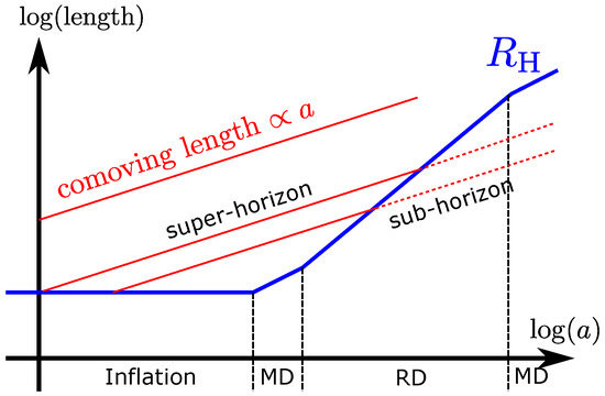
Figure 1. The rough sketch of the standard evolution of the background universe and the perturbations on it.

2.3. Super-Horizon Inhomogeneity

What we mainly discuss in this paper is the black hole formation after the horizon entry during the RD era. Therefore perturbations on super-horizon scales are considered for initial fluctuations of the subsequent evolution of an over-dense region. The evolution of super-horizon perturbations, whose comoving wavenumber k satisfies $k\ll aH$, will be summarized in Section 3. Here let us take a result in advance. At the leading order of the long-wavelength perturbation ($ϵ:=k/\left(aH\right)\ll 1$), we obtain the following metric form:

$$\mathrm{d}{s}^2=-\mathrm{d}{t}^2+a^2\mathsf{\Psi }\left(\mathit{x}\right){\delta }_{ij}\mathrm{d}{x}^i\mathrm{d}{x}^j,$$

(7)

where ${\delta }_{ij}$ is the Kronecker delta and $\mathsf{\Psi }\left(\mathit{x}\right)$ is an arbitrary function of the spatial coordinates $x^i$. It would be fruitful to compare Equation (7) with the metric of the FLRW universe in the isotropic coordinates:

$$\mathrm{d}{s}^2=-\mathrm{d}{t}^2+a^2\frac{1}{{\left(1+\frac{K}{4}{\left|\mathit{x}\right|}^2\right)}^2}{\delta }_{ij}\mathrm{d}{x}^i\mathrm{d}{x}^j.$$

(8)

At the leading order of the long-wavelength approximation, the conformal factor of the spatial metric can be an arbitrary function, that is, the long-wavelength inhomogeneity may be intuitively regarded as the position-dependent spatial curvature. Since a sufficiently overdense region is expected to have a moment of maximum expansion and start to contract, such a region may be considered to have locally positive curvature.

2.4. Three-Zone Model

Motivated by the previous subsection, let us consider the three-zone model composed of the spherical closed FLRW region $r<r_{\mathrm{c}}$ surrounded by an under-dense region embedded in the flat FLRW background (Figure 2).

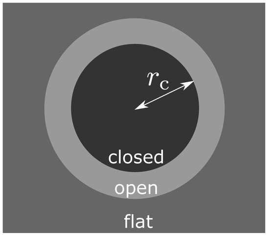
Figure 2. Schematic figure of the three-zone model.

This model can be an exact solution only for the dust case ($w=0$)1. In the case of $w\ne 0$, the pressure gradient force diverges on the discontinuous spheres, and a singular shell must be introduced to realize the configuration as a solution of the Einstein equations. Nevertheless, the three-zone model is useful to intuitively understand the PBH formation process and roughly estimate the threshold for the amplitude of the density perturbation at the horizon entry.

Let us take uniform Hubble time slices and compare the Friedmann Equation (2) in the overdense region and the flat background. On a uniform Hubble time slice, since the value of the Hubble expansion rate is identical, we obtain

$$\frac{8}{3}\pi {\rho }_{\mathrm{b}}=\frac{8}{3}\pi \rho -\frac{K}{a^2},$$

(9)

where $\rho$ and ${\rho }_{\mathrm{b}}$ denote the density in the overdense and background regions, respectively. The overdense region is described by the closed FLRW with the spatial curvature K. From Equation (9), the density perturbation can be calculated as

$$\delta :=\frac{\rho -{\rho }_{\mathrm{b}}}{{\rho }_{\mathrm{b}}}=\frac{K}{a^2{H}^2}.$$

(10)

The value of the density perturbation ${\delta }_{\mathrm{H}}$ at the horizon entry $R_{\mathrm{c}}:=a{r}_{\mathrm{c}}=1/H$ is given by

$${\delta }_{\mathrm{H}}=K{r}_{\mathrm{c}}^2.$$

(11)

Since the value of the comoving radius r cannot be larger than $\sqrt{K}$, we find the following geometrical upper bound [69]:

$${\delta }_{\mathrm{H}}<1.$$

(12)

2.5. Jeans Criterion

If the whole dynamics of the overdense region are described by the closed FLRW universe, nothing prevents the contraction of the closed universe and arbitrarily small amplitude of the positive density perturbation results in black hole formation. However, in reality, the pressure gradient would work as a preventing factor against the contraction. In order to estimate the effect of the pressure gradient, let us apply the Jeans criterion to the three-zone model. The Jeans criterion states that, if the free-fall time scale of the system is shorter than the sound-wave propagation time scale, the gravitational collapse cannot be prevented by the pressure gradient. For the overdense region, the sound-wave propagation time-scale $t_{\mathrm{s}}$ would be given by

$$t_{\mathrm{s}}=\frac{R_{\mathrm{c}}}{\sqrt{w}}=\frac{a{r}_{\mathrm{c}}}{\sqrt{w}}\propto a,$$

(13)

where we have used the fact that the sound speed $c_{\mathrm{s}}$ is given by $\sqrt{w}$. The free-fall time-scale $t_{\mathrm{ff}}$ is given by

$$t_{\mathrm{ff}}=\frac{1}{H}={\left(\frac{8\pi }{3}\rho \right)}^{-1/2}=\frac{a_{\max }}{\sqrt{K}}{\left(\frac{a}{a_{\max }}\right)}^{3(1+w)/2}\propto a^{3(1+w)/2}.$$

(14)

Let us define $a_{\mathrm{th}}$ as the value of the scale factor satisfying $t_{\mathrm{s}}{{|}_{a=a_{\mathrm{th}}}=t_{\mathrm{ff}}|}_{a=a_{\mathrm{th}}}$. Then if $a_{\max }>a_{\mathrm{th}}$, the sound-wave propagation time scale is shorter than the free-fall time scale at the time $a=a_{\max }$, and the gravitational contraction would be prevented by the pressure gradient effect. For the gravitational collapse and black hole formation to be realized, the following condition must be satisfied:

$$a_{\max }<a_{\mathrm{th}}=a_{\max }{\left(\frac{w}{K{r}_{\mathrm{c}}^2}\right)}^{-1/(1+3w)}\iff K{r}_{\mathrm{c}}^2={\delta }_{\mathrm{H}}>w.$$

(15)

This condition is often quoted as Carr’s condition [70]. Here it should be noted that Carr’s condition has the ambiguity of a factor of $\mathcal{O}\left(1\right)$ coming from the order estimations of Equations (13) and (14).

2.6. Refinement of the Threshold

Let us fix the ambiguous factor contained in Carr’s condition (15) based on a well-motivated way [31] and make the condition more reliable. The basic idea is straightforward. We strictly define $t_{\mathrm{s}}$ and $t_{\mathrm{ff}}$ and explicitly calculate these time-scales based on the three-zone model. To do that, let us rewrite the metric of the overdense region in terms of the new radial coordinate $\chi$ defined by

$${sin}^2\left(\sqrt{K}\chi \right)=K{r}^2$$

(16)

as follows:

$$\begin{array}{ccc}\hfill \mathrm{d}{s}^2& =& -\mathrm{d}{t}^2+a^2\left[\mathrm{d}{\chi }^2+\frac{1}{K}{sin}^2\left(\sqrt{K}\chi \right)\mathrm{d}{\Omega }^2\right],\hfill \end{array}$$

(17)

$$\begin{array}{ccc}& =& a^2\left[-\mathrm{d}{\eta }^2+\mathrm{d}{\chi }^2+\frac{1}{K}{sin}^2\left(\sqrt{K}\chi \right)\mathrm{d}{\Omega }^2\right],\hfill \end{array}$$

(18)

where we have also introduced the conformal time defined by $a\mathrm{d}\eta =\mathrm{d}t$. The Friedmann equation can be written as

$${\left[\frac{\mathrm{d}}{\mathrm{d}\eta }lna\right]}^2=K\left[{\left(\frac{a}{a_{\max }}\right)}^{-1-3w}-1\right].$$

(19)

Introducing $u:={(a/a_{\max })}^{1+3w}$, we obtain

$${\left(\frac{\mathrm{d}u}{\mathrm{d}\eta }\right)}^2=K{(1+3w)}^2\left(u-u^2\right).$$

(20)

The solution is given by

$$u=\frac{1}{2}\left[1-cos\left(\sqrt{K}(1+3w)\eta \right)\right],$$

(21)

where the value of $\eta$ is restricted to

$$0\le \eta /2\le {\eta }_{\max }:=\frac{\pi }{\sqrt{K}(1+3w)}.$$

(22)

The times $\eta =0$ and $\eta =2{\eta }_{\max }$ correspond to the big-bang and big-crunch, and the maximum expansion is realized at $\eta ={\eta }_{\max }$. A spacetime diagram for the closed universe with $w=1/3$ is shown in Figure 3.

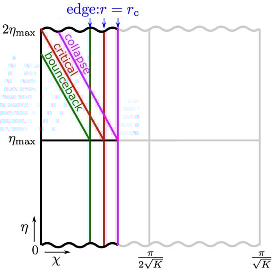
Figure 3. Spacetime diagram for the closed universe with $w=1/3$ describing the overdense region and the trajectory of the sound wave propagation from the edge to the center emanated at the time of the maximum expansion.

Let us reinterpret the Jeans criterion. The propagation time scale of the sound wave can be defined as the time required for the sound wave to propagate from the edge of the overdense region to the center. The free-fall time scale can be simply replaced by the collapsing time of the closed universe describing the overdense region. Therefore if the sound wave emanated from the edge of the overdense region at the time of the maximum expansion reaches the center before the big crunch, we conclude that the gravitational collapse will be prevented by the pressure gradient effect.

The sound speed $c_{\mathrm{s}}$ is given by $c_{\mathrm{s}}=\sqrt{w}$. Then the trajectory of the sound wave is parallel to the straight line $\chi =\pm \sqrt{w}\eta$. From Figure 3, we find that the Jeans criterion gives the threshold of the radius of the closed universe describing the overdense region for PBH formation. This is quite reasonable because the edge radius $r_{\mathrm{c}}$ is related to the amplitude of the density perturbation at the horizon entry by Equation (11). The threshold value is calculated by the following equation:

$$\sqrt{w}{\eta }_{\max }={\chi }_{\mathrm{c}},$$

(23)

where ${\chi }_{\mathrm{c}}$ is the value of the coordinate $\chi$ at the edge of the overdense region, that is, defined by

$${sin}^2\sqrt{K}{\chi }_{\mathrm{c}}=\sqrt{K}{r}_{\mathrm{c}}.$$

(24)

Combining Equations (11), (22)–(24), we can derive the following threshold value for the amplitude of the density perturbation at the horizon entry:

$${\delta }_{\mathrm{th}}={sin}^2\left(\frac{\pi \sqrt{w}}{1+3w}\right).$$

(25)

It should be noted that this value is for the density perturbation in the uniform Hubble gauge. In the comoving gauge, as will be shown later, the factor $3(1+w)/(5+3w)$ must be multiplied, namely,

$${\delta }_{\mathrm{th}}^{\mathrm{co}}=\frac{3(1+w)}{(5+3w)}{sin}^2\left(\frac{\pi \sqrt{w}}{1+3w}\right).$$

(26)

In this section, we have refined Carr’s condition based on the three-zone model. However, our estimation does not go much beyond order estimation. For more rigorous quantitative estimation, we need to rely on numerical simulations, and the threshold value somewhat depends on the profile of the inhomogeneity. Nevertheless, it has been reported that the threshold (26) approximately reproduces the lower bound of the threshold value [35]. Therefore, in terms of results, the three-zone model roughly provides the least possible effect of the pressure gradient against PBH formation.

3. Cosmological Long-Wavelength Solutions

To investigate PBH formation more accurately, we need to investigate the inhomogeneities which are initially super-horizon scales. Such inhomogeneities are described by growing mode solutions in the long-wavelength approximation. The expansion of the long-wavelength approximation with the expansion parameter $ϵ=k/\left(aH\right)$ is often called gradient expansion. In the context of PBH formation, there are two main formulations of gradient expansion. One is the gradient expansion of the equations in the Misner–Sharp formulation [71] in which the Einstein equations for a fluid system in spherical symmetry are written down with the comoving coordinates. The other is based on the cosmological 3 + 1 decomposition [28]. The relation between these two formulations is investigated in Ref. [34]. Although the Misner–Sharp formulation has been adopted for PBH studies by many authors including Polnarev and Musco [72], in this paper, we review the formulation adopted in Ref. [28] because the latter allows more general gauge conditions. We follow and quote the discussions and calculations in Refs. [28,34] in this section. Let us start with writing down the Einstein equations in the form of the cosmological 3 + 1 decomposition for a perfect fluid component. We just display the necessary equations for later discussions and ask readers to refer to Ref. [34] for more details.

3.1. Cosmological 3 + 1 Decomposition

First, we write the line element of spacetime as follows:

$$\mathrm{d}{s}^2=-{\alpha }^2\mathrm{d}{t}^2+a^2{\psi }^4{\tilde{\gamma }}_{ij}(\mathrm{d}{x}^i+{\beta }^i\mathrm{d}t)(\mathrm{d}{x}^j+{\beta }^j\mathrm{d}t),$$

(27)

where a is the scale factor of the background universe, and the lapse function $\alpha$, shift vector ${\beta }^i$, spatial conformal factor $\psi$ and ${\tilde{\gamma }}_{ij}$ are functions of t and $x^i$. We choose ${\tilde{\gamma }}_{ij}$ so that $\tilde{\gamma }:=det\left({\tilde{\gamma }}_{ij}\right)=f:=det\left(f_{ij}\right)$, with $f_{ij}$ being a time-independent metric of the flat three-space. The Latin indices run over 1 to 3 and we drop and raise the Latin indices of quantities without/with tilde by ${\gamma }_{ij}$/${\tilde{\gamma }}_{ij}$ and ${\gamma }^{ij}$/${\tilde{\gamma }}^{ij}$, respectively. The extrinsic curvature of a time slice can be decomposed as

$$K_{ij}={\psi }^4{a}^2\left({\tilde{A}}_{ij}+\frac{1}{3}{\tilde{\gamma }}_{ij}K\right),$$

(28)

where ${\tilde{A}}_{ij}$ satisfies

$${\tilde{\gamma }}^{ij}{\tilde{A}}_{ij}=0.$$

(29)

Then the Hamiltonian and momentum constraint equations can be written as follows:

$$\begin{array}{ccc}& & \tilde{\mathsf{\Delta }}\psi =\frac{1}{8}{\tilde{\mathcal{R}}}_k^k\psi -2\pi {\psi }^5{a}^{2}E-\frac{1}{8}{\psi }^5{a}^2\left({\tilde{A}}_{ij}{\tilde{A}}^{ij}-\frac{2}{3}{K}^2\right),\hfill \end{array}$$

(30)

$$\begin{array}{ccc}& & {\tilde{\mathcal{D}}}^j\left({\psi }^6{\tilde{A}}_{ij}\right)-\frac{2}{3}{\psi }^6{\tilde{\mathcal{D}}}_{i}K=8\pi J_i{\psi }^6,\hfill \end{array}$$

(31)

where $E=n_{\mu }{n}_{\nu }{T}^{\mu \nu }$ and $J_i=-{\gamma }_{i\mu }{n}_{\nu }{T}^{\mu \nu }$ with $n_{\mu }$, ${\gamma }_{\mu \nu }$ and $T^{\mu \nu }$ being the unit-normal form of the time slice, spatial metric and stress-energy tensor, respectively. $\tilde{\mathsf{\Delta }}$, ${\tilde{\mathcal{D}}}_i$ and ${\tilde{\mathcal{R}}}_{ij}$ are the Laplacian, covariant derivative and the Ricci tensor for ${\tilde{\gamma }}_{ij}$, respectively. The evolution equations for geometrical variables are given by

$$\begin{array}{ccc}\hfill ({\partial }_t-{\mathcal{L}}_{\beta }){\tilde{\gamma }}_{ij}& =& -2\alpha {\tilde{A}}_{ij}-\frac{2}{3}{\tilde{\gamma }}_{ij}{\mathcal{D}}_k{\beta }^k,\hfill \end{array}$$

(32)

$$\begin{array}{ccc}\hfill ({\partial }_t-{\mathcal{L}}_{\beta }){\tilde{A}}_{ij}& =& \frac{1}{a^2{\psi }^4}\left[\alpha \left({\mathcal{R}}_{ij}-\frac{{\gamma }_{ij}}{3}\mathcal{R}\right)-\left(D_i{D}_j\alpha -\frac{{\gamma }_{ij}}{3}{D}_k{D}^k\alpha \right)\right]\hfill \\ & & +\alpha (K{\tilde{A}}_{ij}-2{\tilde{A}}_{ik}{\tilde{A}}_j^k)-\frac{2}{3}\left({\mathcal{D}}_k{\beta }^k\right){\tilde{A}}_{ij}-\frac{8\pi \alpha }{a^2{\psi }^4}\left(S_{ij}-\frac{{\gamma }_{ij}}{3}{S}_k^k\right),\hfill \end{array}$$

(33)

$$\begin{array}{ccc}\hfill ({\partial }_t-{\mathcal{L}}_{\beta })\psi & =& -\frac{1}{2}H\psi +\frac{\psi }{6}(-\alpha K+{\mathcal{D}}_k{\beta }^k),\hfill \end{array}$$

(34)

$$\begin{array}{ccc}\hfill ({\partial }_t-{\mathcal{L}}_{\beta })K& =& \alpha \left({\tilde{A}}_{ij}{\tilde{A}}^{ij}+\frac{1}{3}{K}^2\right)-D_k{D}^k\alpha +4\pi \alpha (E+S_k^k),\hfill \end{array}$$

(35)

where $D_i$ and ${\mathcal{D}}_i$ are the covariant derivatives for ${\gamma }_{ij}$ and the three-dimensional flat metric $f_{ij}$, respectively, and ${\mathcal{R}}_{ij}$ is the Ricci tensor for ${\gamma }_{ij}$. $S_{ij}$ is defined by ${\gamma }_{i\mu }{\gamma }_{j\nu }{T}^{\mu \nu }$.

For a perfect fluid, the stress-energy tensor can be written as

$$T_{\mu \nu }=(\rho +p)u_{\mu }{u}_{\nu }+p{g}_{\mu \nu },$$

(36)

where $u^{\mu }$ is the four-velocity of the fluid element which is normalized as $u^{\mu }{u}_{\mu }=-1$. Introducing

$$v^l:=\frac{u^l}{u^t}$$

(37)

and

$$\mathsf{\Gamma }:=\alpha u^t={\left[1-{\alpha }^{-2}({\beta }_k+v_k)({\beta }^k+v^k)\right]}^{-1/2},$$

(38)

we can write the hydrodynamical equations in the form

$$\begin{array}{ccc}& & {\left[{\psi }^6{a}^3\left\{(\rho +p){\mathsf{\Gamma }}^2-p\right\}\right]}_{,t}+\frac{1}{\sqrt{f}}{\left[\sqrt{f}{\psi }^6{a}^3\left\{(\rho +p){\mathsf{\Gamma }}^2-p\right\}{v}^l\right]}_{,l}\hfill \\ & =& -\frac{1}{\sqrt{f}}{\left[\sqrt{f}{\psi }^6{a}^{3}p(v^l+{\beta }^l)\right]}_{,l}+\alpha {\psi }^6{a}^{3}pK-{\alpha }^{-1}{\alpha }_{,l}{\psi }^6{a}^3{\mathsf{\Gamma }}^2(\rho +p)(v^l+{\beta }^l)\hfill \\ & & +{\alpha }^{-1}{\psi }^{10}{a}^5{\mathsf{\Gamma }}^2(\rho +p)(v^l+{\beta }^l)(v^m+{\beta }^m)\left({\tilde{A}}_{lm}+\frac{{\tilde{\gamma }}_{lm}}{3}K\right),\hfill \end{array}$$

(39)

$$\begin{array}{ccc}& & {\left(\mathsf{\Gamma }{\psi }^6{a}^3(\rho +p)u_j\right)}_{,t}+\frac{1}{\sqrt{f}}{\left(\sqrt{f}\mathsf{\Gamma }{\psi }^6{a}^3(\rho +p)v^k{u}_j\right)}_{,k}\hfill \\ & =& -\alpha {\psi }^6{a}^3{p}_{,j}+\mathsf{\Gamma }{\psi }^6{a}^3(\rho +p)\left(-\mathsf{\Gamma }{\alpha }_{,j}+u_k{\beta }_{,j}^k-\frac{u_k{u}_l}{2u^t}{\gamma }_{,j}^{kl}\right),\hfill \end{array}$$

(40)

and

$$\begin{array}{c}\hfill {\left(\mathsf{\Gamma }{\psi }^6{a}^{3}n\right)}_{,t}+\frac{1}{\sqrt{f}}{\left(\sqrt{f}\mathsf{\Gamma }{\psi }^6{a}^{3}n{v}^k\right)}_{,k}=0.\end{array}$$

(41)

3.2. Gradient Expansion

In practice, the gradient expansion is performed by replacing the spatial derivative ${\partial }_i$ by $ϵ{\partial }_i$ with a fictitious parameter $ϵ$. Expanding the equations of motion in a power series of $ϵ$, finally, we set $ϵ=1$. Letting k be the comoving wavenumber for the scale of inhomogeneity of interest, we may consider $|{\partial }_i|\sim k$. Since the only natural scale of the system other than k is H, the fictitious parameter can be regarded as $ϵ\sim k/\left(aH\right)$. We also have to make key assumptions for the leading order $ϵ\to 0$ to perform the gradient expansion. At the leading order, we assume that the universe is given by a spatially flat FLRW universe. More specifically, we require $\alpha -1=\mathcal{O}\left(ϵ\right)$, ${\beta }^i=\mathcal{O}\left(ϵ\right)$ and ${\partial }_t{\tilde{\gamma }}_{ij}=\mathcal{O}\left(ϵ\right)$. In addition, we assume that $\psi$ is identically unity somewhere in the universe, so that $a\left(t\right)$ is the scale factor for that part of the universe. Under these assumptions, it has been shown that ${\partial }_t{\tilde{\gamma }}_{ij}$ temporally decays and one can set ${\partial }_t{\tilde{\gamma }}_{ij}=\mathcal{O}\left({ϵ}^2\right)$ for growing mode solutions [73].

In this review, we mainly focus on two specific time slicing conditions: the constant mean curvature (CMC) slicing ($K=-3H$) and comoving slicing ($n^{\mu }=u^{\mu }$). Readers may refer to Ref. [34] for other gauge conditions. The comoving slicing implies $u_i=u^t(v_i+{\beta }_i)=0$, then $\mathsf{\Gamma }=1$, $E=\rho$ and $J_i=(\rho +p)u_i=0$. Since ${\tilde{A}}_{ij}=\mathcal{O}\left({ϵ}^2\right)$ from Equation (32), from the momentum (31) and Hamiltonian (30) constraints, we obtain ${\tilde{\mathcal{D}}}_{i}K=\mathcal{O}\left({ϵ}^3\right)$ and $H^2=\frac{8\pi }{3}\rho +\mathcal{O}\left({ϵ}^2\right)$. Therefore CMC, uniform density and comoving slicings coincide to $\mathcal{O}\left(ϵ\right)$. In addition, from Equation (39), we obtain

$$2{\partial }_{t}ln\psi =H-{\partial }_{t}lna+\mathcal{O}\left({ϵ}^2\right),$$

(42)

where we have assumed that the pressure is homogeneous to $\mathcal{O}\left(ϵ\right)$. Since the right-hand side is a function of t, ${\partial }_{t}ln\psi$ is also homogeneous to $\mathcal{O}\left(ϵ\right)$. Since we have assumed that $\psi$ is identically unity at some point, we conclude

$${\partial }_t\psi =\mathcal{O}\left({ϵ}^2\right).$$

(43)

Coming back to the general expressions without specifying the slicing condition, from ${\partial }_t\psi =\mathcal{O}\left({ϵ}^2\right)$ and the equations of motion displayed in the previous section, one can find

$$\begin{array}{ccc}& & \psi =\mathcal{O}\left({ϵ}^0\right),v^i=\mathcal{O}\left(ϵ\right),\rho ={\rho }_{\mathrm{b}}(1+\mathcal{O}\left({ϵ}^2\right)),{\tilde{A}}_{ij}=\mathcal{O}\left({ϵ}^2\right),\hfill \\ & & {\tilde{\gamma }}_{ij}=f_{ij}+\mathcal{O}\left({ϵ}^2\right),\alpha =1+\mathcal{O}\left({ϵ}^2\right),K=3H(1+\mathcal{O}\left({ϵ}^2\right)),\hfill \end{array}$$

(44)

where ${\rho }_{\mathrm{b}}$ is the background density. Then we introduce the following perturbation variables:

$$\begin{array}{ccc}\hfill \psi (t,\mathit{x})& =& \mathsf{\Psi }\left(\mathit{x}\right)(1+\xi (t,\mathit{x}))+\mathcal{O}\left({ϵ}^3\right),\hfill \end{array}$$

(45)

$$\begin{array}{ccc}\hfill {\tilde{\gamma }}_{ij}(t,\mathit{x})& =& f_{ij}+h_{ij}(t,\mathit{x})+\mathcal{O}\left({ϵ}^3\right),\hfill \end{array}$$

(46)

$$\begin{array}{ccc}\hfill K(t,\mathit{x})& =& 3H(1+\kappa (t,\mathit{x}))+\mathcal{O}\left({ϵ}^3\right),\hfill \end{array}$$

(47)

$$\begin{array}{ccc}\hfill \alpha (t,\mathit{x})& =& 1+\chi (t,\mathit{x})+\mathcal{O}\left({ϵ}^3\right),\hfill \end{array}$$

(48)

$$\begin{array}{ccc}\hfill {\beta }^i(t,\mathit{x})& =& \mathcal{O}\left(ϵ\right),\hfill \end{array}$$

(49)

$$\begin{array}{ccc}\hfill \rho (t,\mathit{x})& =& {\rho }_{\mathrm{b}}(1+\delta (t,\mathit{x}))+\mathcal{O}\left({ϵ}^3\right),\hfill \end{array}$$

(50)

$$\begin{array}{ccc}\hfill v^i(t,\mathit{x})& =& \mathcal{O}\left(ϵ\right),\hfill \end{array}$$

(51)

where $\mathsf{\Psi }\left(\mathit{x}\right)=\mathcal{O}\left({ϵ}^0\right)$ and $\xi$, $h_{ij}$, $\kappa$, $\chi$ and $\delta$ are the perturbation variables of $\mathcal{O}\left({ϵ}^2\right)$.

Hereafter, we focus on the case of the linear equation of state $p=w\rho$ and consider the normal threading ${\beta }^i=0$ for simplicity. Readers may refer to Ref. [34] for other general cases. The equations of motion can be reduced to the following:

$$\begin{array}{ccc}& & {\partial }_t\delta +3H(1+w)(\chi +\kappa )=O\left({ϵ}^4\right),\hfill \end{array}$$

(52)

$$\begin{array}{ccc}& & {\partial }_t\left[a^3(1+w){\rho }_{\mathrm{b}}{u}_j\right]=-a^3{\rho }_{\mathrm{b}}\left[w{\partial }_j\delta +(1+w){\partial }_j\chi \right]+O\left({ϵ}^5\right),\hfill \end{array}$$

(53)

$$\begin{array}{ccc}& & 6{\partial }_t\xi -3H(\chi +\kappa )=O\left({ϵ}^4\right),\hfill \end{array}$$

(54)

$$\begin{array}{ccc}& & \mathsf{\Delta }\mathsf{\Psi }=-2\pi {\mathsf{\Psi }}^5{a}^2{\rho }_{\mathrm{b}}(\delta -2\kappa )+O\left({ϵ}^4\right),\hfill \end{array}$$

(55)

$$\begin{array}{ccc}& & H^{-1}{\partial }_t\kappa =\frac{1}{2}(3w-1)\kappa -\frac{3}{2}(1+w)\chi -\frac{1}{2}\delta (1+3w)+O\left({ϵ}^4\right),\hfill \end{array}$$

(56)

$$\begin{array}{ccc}& & {\partial }_t{h}_{ij}=-2{\tilde{A}}_{ij}+O\left({ϵ}^4\right),\hfill \end{array}$$

(57)

$$\begin{array}{ccc}& & {\partial }_t{\tilde{A}}_{ij}+3H{\tilde{A}}_{ij}=\frac{1}{a^2{\mathsf{\Psi }}^4}[-\frac{2}{\mathsf{\Psi }}\left({\mathcal{D}}_i{\mathcal{D}}_j\mathsf{\Psi }-\frac{1}{3}{f}_{ij}\mathsf{\Delta }\mathsf{\Psi }\right)\hfill \\ & & +\frac{6}{{\mathsf{\Psi }}^2}\left({\mathcal{D}}_i\mathsf{\Psi }{\mathcal{D}}_j\mathsf{\Psi }-\frac{1}{3}{f}_{ij}{\mathcal{D}}^k\mathsf{\Psi }{\mathcal{D}}_k\mathsf{\Psi }\right)]+O\left({ϵ}^4\right),\hfill \end{array}$$

(58)

$$\begin{array}{ccc}& & {\mathcal{D}}_i\left({\mathsf{\Psi }}^6{\tilde{A}}_j^i\right)+2H{\mathsf{\Psi }}^6{\mathcal{D}}_j\kappa =8\pi {\mathsf{\Psi }}^6(1+w){\rho }_{\mathrm{b}}{u}_j+O\left({ϵ}^5\right),\hfill \end{array}$$

(59)

The solutions for Equations (57) and (58) are given by

$$\begin{array}{ccc}\hfill h_{ij}& =& -\frac{4}{(3w+5)(3w-1)}{p}_{ij}{\left(\frac{1}{aH}\right)}^2+O\left({ϵ}^4\right),\hfill \end{array}$$

(60)

$$\begin{array}{ccc}\hfill {\tilde{A}}_{ij}& =& \frac{2}{3w+5}{p}_{ij}H{\left(\frac{1}{aH}\right)}^2+O\left({ϵ}^4\right),\hfill \end{array}$$

(61)

respectively, where

$$p_{ij}\left(\mathit{x}\right):=\frac{1}{{\mathsf{\Psi }}^4}\left[-\frac{2}{\mathsf{\Psi }}\left({\mathcal{D}}_i{\mathcal{D}}_j\mathsf{\Psi }-\frac{1}{3}{f}_{ij}\mathsf{\Delta }\mathsf{\Psi }\right)+\frac{6}{{\mathsf{\Psi }}^2}\left({\mathcal{D}}_i\mathsf{\Psi }{\mathcal{D}}_j\mathsf{\Psi }-\frac{1}{3}{f}_{ij}{\mathcal{D}}^k\mathsf{\Psi }{\mathcal{D}}_k\mathsf{\Psi }\right)\right]$$

(62)

with $\mathsf{\Delta }:=f^{ij}{\mathcal{D}}_i{\mathcal{D}}_j$.

To find solutions for other quantities, we need to fix the slicing condition. Let us consider CMC slicing ($\kappa =0$). From Equation (55), we obtain

$$\delta =q{\left(\frac{1}{aH}\right)}^2+\mathcal{O}\left({ϵ}^4\right),$$

(63)

where

$$q\left(\mathit{x}\right)=-\frac{4}{3}\frac{\mathsf{\Delta }\mathsf{\Psi }}{\mathsf{\Psi }}.$$

(64)

Then, from Equations (56), (54) and (53), $\chi$, $\xi$ and $u_j$ are given as

$$\begin{array}{ccc}\hfill \chi & =& -\frac{3w+1}{3(1+w)}q{\left(\frac{1}{aH}\right)}^2+\mathcal{O}\left({ϵ}^4\right),\hfill \end{array}$$

(65)

$$\begin{array}{ccc}\hfill \xi & =& -\frac{1}{6(1+w)}q{\left(\frac{1}{aH}\right)}^2+\mathcal{O}\left({ϵ}^4\right),\hfill \end{array}$$

(66)

$$\begin{array}{ccc}\hfill u_j& =& v_j+\mathcal{O}\left({ϵ}^5\right)=\frac{2}{3(1+w)(3w+5)}{\partial }_{j}qa{\left(\frac{1}{aH}\right)}^3+\mathcal{O}\left({ϵ}^5\right).\hfill \end{array}$$

(67)

One can check that the solutions solve the other equations not used to derive the solutions.

For the comoving slicing ($u_j=0$), from Equation (53), we obtain

$$\chi =\frac{w}{1+w}\delta +\mathcal{O}\left({ϵ}^4\right).$$

(68)

Substituting this relation into Equations (52) and (56), and combining them, we can derive the following solutions for $\delta$ and $\kappa$:

$$\begin{array}{ccc}\hfill \delta & =& \frac{3(1+w)}{3w+5}q{\left(\frac{1}{aH}\right)}^2+\mathcal{O}\left({ϵ}^4\right),\hfill \end{array}$$

(69)

$$\begin{array}{ccc}\hfill \kappa & =& -\frac{1}{3w+5}q{\left(\frac{1}{aH}\right)}^2+\mathcal{O}\left({ϵ}^4\right).\hfill \end{array}$$

(70)

Then $\chi$ can be given as

$$\chi =-\frac{3}{3w+5}q{\left(\frac{1}{aH}\right)}^2+\mathcal{O}\left({ϵ}^4\right).$$

(71)

From Equation (54), we obtain

$$\xi =-\frac{1}{2(3w+5)}q{\left(\frac{1}{aH}\right)}^2+\mathcal{O}\left({ϵ}^4\right).$$

(72)

Since the function $\mathsf{\Psi }\left(\mathit{x}\right)$, and therefore $q\left(\mathit{x}\right)$ are shared in the both gauge conditions, we can easily find the relation of gauge-dependent quantities. For instance, we find

$${\delta }_{\mathrm{co}}=\frac{3(1+w)}{3w+5}{\delta }_{\mathrm{CMC}}+\mathcal{O}\left({ϵ}^4\right),$$

(73)

where ${\delta }_{\mathrm{CMC}}$ and ${\delta }_{\mathrm{co}}$ are density perturbations for CMC and comoving gauges, respectively.

4. PBH Formation Criterion

In this section, we consider spherically symmetric systems. In earlier days, the amplitude of the density perturbation averaged within a certain radius is used to give an analytic PBH formation criterion for convenience. More specifically, letting $\overline{\delta }$ be the amplitude of the volume average of the density perturbation at the horizon entry, if $\overline{\delta }$ exceeds a certain threshold value, we think that PBH formation is realized. The threshold value has been estimated analytically and numerically by many authors [27,28,30,31,32,33,70,72,74,75,76,77].

A recent trend is to use the “compaction function” firstly proposed in Ref. [28]. There are several efforts to refine the simple treatment of the compaction function for a more accurate and convenient criterion of PBH formation [35,36,37,38]. In this review, however, to avoid complicated discussions, we do not go into details about the recent refinements, but just review the simple use of the compaction function. That is, if the maximum value of the compaction function exceeds a certain threshold value, we think that PBH formation is realized. In this procedure, the threshold value depends on the profile of the initial perturbation. Nevertheless, we expect that, for moderate profiles, the deviation due to the profile dependence would be about 10%. Regarding the compaction function, recently, we found a misunderstanding that has not been realized for a long time. This misunderstanding will be also resolved.

Let us start with defining Shibata–Sasaki’s original compaction function in terms of the cosmological long-wavelength perturbations as follows:

$${\mathcal{C}}_{\mathrm{SS}}\left(r\right):=\frac{\delta M_{\mathrm{SS}}}{R}\mathrm{with}\delta M_{\mathrm{SS}}:=4\pi a^3{\rho }_{\mathrm{b}}{\int }_0^r\mathrm{d}x{\delta }_{\mathrm{CMC}}{\left({\mathsf{\Psi }}^{2}x\right)}^2\frac{\mathrm{d}}{\mathrm{d}x}\left({\mathsf{\Psi }}^{2}x\right),$$

(74)

where R is the areal radius of the sphere of the coordinate radius r given by $R=ar{\mathsf{\Psi }}^2$. By using the solution (63), one can derive the following expression [34]:

$${\mathcal{C}}_{\mathrm{SS}}\left(r\right)=\frac{1}{2}\left[1-\left(1+2r\frac{\mathrm{d}}{\mathrm{d}r}ln\mathsf{\Psi }\right)\right].$$

(75)

From this expression, we find that ${\mathcal{C}}_{\mathrm{SS}}$ is time independent and calculated by the gauge independent quantity $\mathsf{\Psi }$. Furthermore, $\mathsf{\Psi }$ is related to the curvature perturbation, which is often used in the context of cosmological perturbation in the early universe, as $\zeta =-\frac{1}{2}ln\mathsf{\Psi }$ 2. Let us introduce the radius $r_{\mathrm{m}}$ at which the compaction function takes the maximum value ${\mathcal{C}}_{\mathrm{SS}}^{\max }={\mathcal{C}}_{\mathrm{SS}}\left(r_{\mathrm{m}}\right)$. Then, we adopt the following PBH formation criterion:

$${\mathcal{C}}_{\mathrm{SS}}^{\max }\gtrsim {\mathcal{C}}_{\mathrm{SS}}^{\mathrm{th}}$$

(76)

with the uncertainty coming from the profile dependence. As is shown in Figures 2 and 3 in Ref. [34] for two specific one-parameter families of initial profiles, the value of ${\mathcal{C}}_{\mathrm{th}}$ can be roughly estimated as $0.4$ with about 10% uncertainty. For the specific profile given by $ln\mathsf{\Psi }\propto sin\left(r\right)/r$, which corresponds to the typical profile for the monochromatic power spectrum of $ln\mathsf{\Psi }$, we obtain ${\mathcal{C}}_{\mathrm{th}}\simeq 0.44$ from numerical simulations. Therefore we use the value ${\mathcal{C}}_{\mathrm{th}}=0.44$ as a reference value in this paper.

In order to understand the compaction function more deeply, let us review the relation between the compaction function and the conserved mass. In spherical symmetry, we have a well-behaved conserved mass called Misner–Sharp mass [71]. As is shown in Appendix A, the Misner–Sharp mass is equivalent to the Kodama mass defined by the charge associated with a conserved current. In addition, the value of the Misner–Sharp mass on a marginally trapped surface is given by half of the areal radius of the marginally trapped surface. Therefore the Misner–Sharp mass is closely related to horizon formation, and relevant to be used for horizon formation criterion.

From the expression of the Kodama current and mass given in Equations (A16) and (A19), we can derive the following expression:

$$\begin{array}{ccc}\hfill M(t,r)& =& 4\pi {\int }_0^r\mathrm{d}x{x}^2{a}^3\alpha {\psi }^6{T}_{\mu }^t{K}^{\mu }\hfill \\ & =& 4\pi a^3{\int }_0^r\mathrm{d}x{x}^2{\psi }^4\left\{-[(\rho +p)u^t{u}_t+p]{\partial }_x\left({\psi }^{2}x\right)+(\rho +p)u^t{u}_r\frac{x}{a}{\partial }_t\left({\psi }^{2}a\right)\right\}.\hfill \end{array}$$

(77)

In the comoving slice ($u_r=0$), we obtain

$$\begin{array}{ccc}\hfill M_{\mathrm{co}}(t,r)& =& 4\pi a^3{\int }_0^r\mathrm{d}x{x}^2{\psi }^4\rho \left\{{\partial }_x\left({\psi }^{2}x\right)+\mathcal{O}\left({ϵ}^4\right)\right\}.\hfill \end{array}$$

(78)

The mass excess compared to the background FLRW with the identical areal radius is calculated as

$$\delta M_{\mathrm{co}}:=M(t,r)-M_{\mathrm{FLRW}}(t,{\psi }^{2}r)=4\pi a^3{\rho }_{\mathrm{b}}{\int }_0^r\mathrm{d}x\left[{\left({\mathsf{\Psi }}^{2}x\right)}^2{\partial }_x\left({\mathsf{\Psi }}^{2}x\right){\delta }_{\mathrm{co}}+\mathcal{O}\left({ϵ}^4\right)\right].$$

(79)

Then we can define the compaction function in the comoving gauge as

$${\mathcal{C}}_{\mathrm{co}}:=\frac{\delta M_{\mathrm{co}}}{R}=\frac{3(1+w)}{3w+5}\frac{1}{2}\left[1-(1+2r{\partial }_{r}ln\mathsf{\Psi })\right]=\frac{3(1+w)}{3w+5}{\mathcal{C}}_{\mathrm{SS}},$$

(80)

where $R=a{\mathsf{\Psi }}^{2}r$. Therefore ${\mathcal{C}}_{\mathrm{SS}}$ is the compaction function in the comoving gauge multiplied by $\frac{3(1+w)}{3w+5}$. However, it should be noted that, for the CMC slice, the contribution from the second term in the integrand of Equation (77) cannot be neglected3 and we find ${\mathcal{C}}_{\mathrm{CMC}}\ne {\mathcal{C}}_{\mathrm{SS}}$. More concrete description will be reported elsewhere.

To see the relation between the compaction function and the volume average of the density perturbation, let us define the volume average of the density perturbation in the comoving slice as follows:

$$\overline{\delta }:=\frac{4\pi {\int }_0^r\mathrm{d}x{\left({\mathsf{\Psi }}^{2}x\right)}^2{\partial }_x\left({\mathsf{\Psi }}^{2}x\right){\delta }_{\mathrm{co}}}{4\pi {\left({\mathsf{\Psi }}^{2}r\right)}^3/3}.$$

(81)

Then we can easily find

$$\overline{\delta }=\frac{2}{H^2{R}^2}\frac{\delta M_{\mathrm{co}}}{R}.$$

(82)

Therefore we obtain

$${\left.\overline{\delta }\right|}_{HR=1}=2{\mathcal{C}}_{\mathrm{co}}.$$

(83)

That is, the compaction function can be also regarded as the amplitude of the volume average of the density perturbation at the horizon entry. This relation also supports the relevance of the compaction function to be used for the criterion of PBH formation.

5. Estimation of PBH Abundance in Peak Theory

We start with writing the spatial metric in the following form:

$$\mathrm{d}{s}_3^2=a^2{\mathrm{e}}^{-2\zeta }{\tilde{\gamma }}_{ij}\mathrm{d}{x}^i\mathrm{d}{x}^j.$$

(84)

The curvature perturbation $\zeta$ is related to $\mathsf{\Psi }$ as

$$\zeta =-\frac{1}{2}ln\mathsf{\Psi }.$$

(85)

Here we assume that $\zeta$ is the Gaussian random variable with the power spectrum $\mathcal{P}\left(k\right)$ defined by

$$⟨{\tilde{\zeta }}^{*}\left(\mathit{k}\right)\tilde{\zeta }\left({\mathit{k}}^{\prime }\right)⟩=\frac{2{\pi }^2}{k^3}\mathcal{P}\left(k\right){\left(2\pi \right)}^3\delta (\mathit{k}-{\mathit{k}}^{\prime })$$

(86)

with $\tilde{\zeta }\left(\mathit{k}\right)=\int {\mathrm{d}}^{3}x\zeta \left(\mathit{x}\right){\mathrm{e}}^{\mathrm{i}\mathit{k}\mathit{x}}$. Readers may refer to Refs. [78,79,80] for non-Gaussian cases. From the random Gaussian assumption and the gradient moments ${\sigma }_n$ given by

$${\sigma }_n^2=\int \mathrm{d}lnk{k}^{2n}\mathcal{P}\left(k\right),$$

(87)

as is shown in Appendix B, Appendix C and Appendix D, we can obtain the peak number density $n_{\mathrm{pk}}^{\left(k_{•}\right)}({\tilde{\mu }}_2,k_{•})$ and the typical peak profile $\overline{\zeta }\left(r\right)$ characterized by the two parameters ${\tilde{\mu }}_2$ and $k_{•}$ defined by

$$\begin{array}{ccc}\hfill {\tilde{\mu }}_2& =& \mathsf{\Delta }\zeta \left(0\right)\frac{{\sigma }_1^2}{{\sigma }_2^2},\hfill \end{array}$$

(88)

$$\begin{array}{ccc}\hfill k_{•}^2& =& -\frac{\mathsf{\Delta }\mathsf{\Delta }\zeta \left(0\right)}{{\tilde{\mu }}_2}\frac{{\sigma }_1^2}{{\sigma }_2^2},\hfill \end{array}$$

(89)

where Δ is the flat Laplacian. Here we just write down the final expressions (A76) and (A78):

$$\begin{array}{ccc}\hfill n_{\mathrm{pk}}^{\left(k_{•}\right)}({\tilde{\mu }}_2,k_{•})d{\tilde{\mu }}_{2}d{k}_{•}=\frac{2·3^{3/2}}{{\left(2\pi \right)}^{3/2}}{\tilde{\mu }}_2{k}_{•}\frac{{\sigma }_2^3{\sigma }_4^2}{{\sigma }_1^4{\sigma }_3^3}f\left({\tilde{\mu }}_2{k}_{•}^2\frac{{\sigma }_2^2}{{\sigma }_1^2{\sigma }_4}\right)P_1\left({\tilde{\mu }}_2\frac{{\sigma }_2}{{\sigma }_1^2},{\mu }_2{k}_{•}^2\frac{{\tilde{\sigma }}_2^2}{{\sigma }_1^2{\sigma }_4};{\gamma }_3\right)\mathrm{d}{\tilde{\mu }}_2\mathrm{d}{k}_{•},& & \hfill \end{array}$$

(90)

$$\begin{array}{ccc}\hfill \frac{\overline{\zeta }\left(r\right)}{{\tilde{\mu }}_2}=-\frac{1}{1-{\gamma }_3^2}\left({\psi }_1+\frac{1}{3}{R}_3^2\mathsf{\Delta }{\psi }_1\right)+k_{•}^2\frac{1}{{\gamma }_3(1-{\gamma }_3^2)}\frac{{\sigma }_2}{{\sigma }_4}\left({\gamma }_3^2{\psi }_1+\frac{1}{3}{R}_3^2\mathsf{\Delta }{\psi }_1\right),& & \hfill \end{array}$$

(91)

where $P_1$, f, $R_n$ and ${\psi }_n$ are defined in Equations (A38), (A50), (A71) and (A75), respectively, and we omitted the last term in (A77), which can be absorbed into the renormalization of the scale factor.

A flow chart to reach the PBH mass spectrum by using the peak number density (90), typical profile (91) and the PBH formation criterion (76) is shown in Figure 4. Let us explain each step of the flow chart.

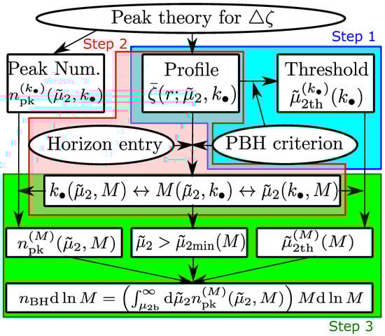
Figure 4. A flow chart to reach the PBH mass spectrum.

5.1. Step 1: Rewriting the Criterion

First, let us consider the compaction function for the typical profile. Hereafter we will work in the comoving gauge and express the compaction function in the comoving gauge without the subscript, that is, $\mathcal{C}={\mathcal{C}}_{\mathrm{co}}$. Focusing on the radiation-dominated universe ($w=1/3$), the PBH formation criterion can be rewritten as

$${\mathcal{C}}^{\max }=\mathcal{C}\left(r_{\mathrm{m}}\right)=\frac{2}{3}{\mathcal{C}}_{\mathrm{SS}}^{\max }\gtrsim {\mathcal{C}}^{\mathrm{th}}\sim 0.293$$

(92)

In terms of the typical profile $\overline{\zeta }$, the compaction function can be written as

$$\mathcal{C}=\frac{1}{3}\left[1-{\left(1-r{\partial }_r\overline{\zeta }\right)}^2\right].$$

(93)

Assuming type I fluctuations defined by ${\partial }_{r}R>0\Rightarrow {\partial }_r\left({\mathrm{e}}^{-\zeta }r\right)>0$, we obtain

$$\left({\partial }_r\overline{\zeta }+r{\partial }_r^2\zeta \right){|}_{r=r_{\mathrm{m}}}=0.$$

(94)

Defining the function $g(r;k_{•})$ by

$$g(r;k_{•}):=\frac{\overline{\zeta }\left(r\right)}{{\tilde{\mu }}_2},$$

(95)

the condition (94) for $r_{\mathrm{m}}$ can be rewritten as

$$({\partial }_{r}g+r{\partial }_r^{2}g){|}_{r=r_{\mathrm{m}}}=0.$$

(96)

This equation implicitly gives the value of $r_{\mathrm{m}}$ as a function of $k_{•}$: $r_{\mathrm{m}}=r_{\mathrm{m}}\left(k_{•}\right)$. The value ${\mathcal{C}}^{\max }$ is then given as a function of ${\tilde{\mu }}_2$ and $k_{•}$ through $r_{\mathrm{m}}\left(k_{•}\right)$ as

$${\tilde{\mu }}_2=\frac{1-\sqrt{1-3{\mathcal{C}}_{\max }}}{r_{\mathrm{m}}{\partial }_{r}g\left(r_{\mathrm{m}}\right)}.$$

(97)

Through this equation, we can obtain the threshold value of ${\tilde{\mu }}_2$ as a function of $k_{•}$ as

$${\tilde{\mu }}_{2\mathrm{th}}^{\left(k_{•}\right)}\left(k_{•}\right):=\frac{1-\sqrt{{\mathcal{C}}_{\mathrm{th}}}}{r_{\mathrm{m}}\left(k_{•}\right){\partial }_r{g}_{\mathrm{m}}\left(k_{•}\right)},$$

(98)

where ${\partial }_r{g}_{\mathrm{m}}={\partial }_{r}g(r_{\mathrm{m}}\left(k_{•}\right);k_{•})$.

5.2. Step 2: Derivation of the PBH Mass Expression

In order to obtain the number density for a fixed PBH mass, we need to know the relation between the parameters ${\tilde{\mu }}_2$, $k_{•}$ and the PBH mass M. The typical mass of a PBH can be roughly estimated by the horizon mass of $1/\left(2H\right)$ at the horizon entry. The horizon entry condition is given by

$$aH=\frac{a}{R}=\frac{{\mathrm{e}}^{{\tilde{\mu }}_2{g}_{\mathrm{m}}}}{r_{\mathrm{m}}}.$$

(99)

In the radiation-dominated universe, adopting the matter-radiation equality as a reference time, we find

$$a=a_{\mathrm{eq}}{\left(\frac{H_{\mathrm{eq}}}{H}\right)}^{1/2}.$$

(100)

From Equations (99) and (100), at the horizon entry, we obtain

$$H^{-1}=a_{\mathrm{eq}}^2{H}_{\mathrm{eq}}{r}_{\mathrm{m}}^2{\mathrm{e}}^{-2{\tilde{\mu }}_2{g}_{\mathrm{m}}}=H_{\mathrm{eq}}^{-1}{k}_{\mathrm{eq}}^2{r}_{\mathrm{m}}^2{\mathrm{e}}^{-2{\tilde{\mu }}_2{g}_{\mathrm{m}}},$$

(101)

where $k_{\mathrm{eq}}=a_{\mathrm{eq}}{H}_{\mathrm{eq}}$. Then the PBH mass can be estimated as

$$M=\frac{1}{2H}=\frac{1}{2}{H}_{\mathrm{eq}}^{-1}{k}_{\mathrm{eq}}^2{r}_{\mathrm{m}}^2{\mathrm{e}}^{-2{\tilde{\mu }}_2{g}_{\mathrm{m}}}=M_{\mathrm{eq}}{k}_{\mathrm{eq}}^2{r}_{\mathrm{m}}^2{\mathrm{e}}^{-2{\tilde{\mu }}_2{g}_{\mathrm{m}}},$$

(102)

where we have introduced $M_{\mathrm{eq}}=1/\left(2H_{\mathrm{eq}}\right)$. We have not taken into account the mass scaling associated with the critical behavior [81,82] in the expression (102). It should be also noted that the mass estimation given in this paper cannot be applied to Type II PBH formation [69].

5.3. Step 3: Derivation of the Mass Function

Equation (106) gives us the relation between M, $k_{•}$ and ${\tilde{\mu }}_2$. Therefore we can change the independent variables in the peak number density (90) from ${\tilde{\mu }}_2$ and $k_{•}$ to ${\tilde{\mu }}_2$ and M as follows:

$$\begin{array}{ccc}\hfill n_{\mathrm{pk}}^{\left(M\right)}({\tilde{\mu }}_2,M)d{\tilde{\mu }}_{2}dlnM& =& \frac{2·3^{3/2}}{{\left(2\pi \right)}^{3/2}}{\tilde{\mu }}_2{k}_{•}\frac{{\sigma }_2^3{\sigma }_4^2}{{\sigma }_1^4{\sigma }_3^3}f\left({\tilde{\mu }}_2{k}_{•}^2\frac{{\sigma }_2^2}{{\sigma }_1^2{\sigma }_4}\right)\hfill \\ & & P_1\left({\tilde{\mu }}_2\frac{{\sigma }_2}{{\sigma }_1^2},{\tilde{\mu }}_2{k}_{•}^2\frac{{\sigma }_2^2}{{\sigma }_1^2{\sigma }_4};{\gamma }_3\right){\left|\frac{\mathrm{d}lnM}{\mathrm{d}{k}_{•}}\right|}^{-1}\mathrm{d}{\tilde{\mu }}_2\mathrm{d}lnM,\hfill \end{array}$$

(103)

where $k_{•}$ should be regarded as a function of ${\tilde{\mu }}_2$ and M through Equation (102). To obtain the PBH number density for a given value of the mass M, we need to integrate Equation (103) for ${\tilde{\mu }}_2$.

As is explicitly shown in Ref. [67] for some specific cases, the threshold value of ${\tilde{\mu }}_2$ given by Equation (98) can be converted to the threshold value ${\tilde{\mu }}_{2\mathrm{th}}^{\left(M\right)}\left(M\right)$ for a given value of M by using Equations (98) and (102). In addition, the value of ${\tilde{\mu }}_2$ may be bounded below for a fixed value of M. Then, letting the minimum possible value of ${\tilde{\mu }}_2$ be ${\tilde{\mu }}_{2\min }\left(M\right)$, the lower limit of the integral for ${\tilde{\mu }}_2$ is given by ${\tilde{\mu }}_{2\mathrm{b}}:=max\left\{{\tilde{\mu }}_{2\min }\left(M\right),{\tilde{\mu }}_{2\mathrm{th}}^{\left(M\right)}\left(M\right)\right\}$. That is, the PBH number density $n_{\mathrm{BH}}\left(M\right)$ and the mass spectrum $f_0\left(M\right)$ at equality time are given by

$$\begin{array}{ccc}\hfill n_{\mathrm{BH}}\mathrm{d}lnM& =& \left[{\int }_{{\tilde{\mu }}_{2\mathrm{b}}}^{\infty }\mathrm{d}{\tilde{\mu }}_2{n}_{\mathrm{pk}}^{\left(M\right)}({\tilde{\mu }}_2,M)\right]\mathrm{d}lnM,\hfill \end{array}$$

(104)

$$\begin{array}{ccc}\hfill f_0\mathrm{d}lnM& =& \frac{M{n}_{\mathrm{BH}}}{\rho a^3}\frac{a_{\mathrm{eq}}}{a}\mathrm{d}lnM=\frac{4\pi }{3}\frac{M}{M_{\mathrm{eq}}}{k}_{\mathrm{eq}}^{-3}{n}_{\mathrm{BH}}\mathrm{d}lnM.\hfill \end{array}$$

(105)

5.4. Critical Behavior

It is well known that, at least for idealized spherically-symmetric situations, the mass of the black hole scales as $\propto {(b-b_{\mathrm{th}})}^{\gamma }$ with b and $b_{\mathrm{th}}$ being one parameter characterizing the initial data and the threshold value of it, respectively. PBH formation is no exception, and its realization and the effects on the PBH abundance have been investigated [26,27,30,76,77,79,83,84,85,86,87]. If we take the critical behavior into account, the PBH mass would be given by

$$M=K\left(k_{•}\right){({\tilde{\mu }}_2-{\tilde{\mu }}_{2\mathrm{th}}^{\left(k_{•}\right)}\left(k_{•}\right))}^{\gamma }{M}_{\mathrm{eq}}{k}_{\mathrm{eq}}^2{r}_{\mathrm{m}}^2{\mathrm{e}}^{-2{\tilde{\mu }}_2{g}_{\mathrm{m}}},$$

(106)

where $\gamma$ is the universal exponent given by $\gamma \simeq 0.36$ for radiation fluid, and $K\left(k_{•}\right)$ is a profile-dependent numerical factor, which will be set to be 1 hereafter for simplicity. In practice, we can consider the case without critical behavior setting the value of $\gamma$ to be 0 in Equation (106).

5.5. The Monochromatic Curvature Power Spectrum

In this paper, we show only the case of the monochromatic curvature power spectrum. Readers may refer to Refs. [66,67] for extended spectra. Let us write the monochromatic power spectrum as

$$\mathcal{P}\left(k\right)={\sigma }_0^2{k}_0\delta (k-k0)={\sigma }_0\delta (lnk-ln{k}_0).$$

(107)

Then the gradient moments are calculated as

$${\sigma }_n^2={\sigma }_0^2{k}_0^{2n}\Rightarrow {\gamma }_n=1.$$

(108)

The typical profile is given as

$$g(r;k_{•})=\frac{\overline{\zeta }}{{\tilde{\mu }}_2}=-{\psi }_1=-\frac{sin\left(k_{0}r\right)}{k_{0}r}.$$

(109)

From the condition (94), we can find

$$r_{\mathrm{m}}\simeq 2.74/k_0,g_{\mathrm{m}}=g\left(r_{\mathrm{m}}\right)\simeq -0.141.$$

(110)

From the condition (92), we can find

$${\tilde{\mu }}_{2\mathrm{th}}\simeq 0.615.$$

(111)

Then the PBH mass can be given by a function of ${\tilde{\mu }}_2$ as

$$M={({\tilde{\mu }}_2-{\tilde{\mu }}_{2\mathrm{th}})}^{\gamma }{M}_{\mathrm{eq}}{k}_{\mathrm{eq}}^2{r}_{\mathrm{m}}^2{\mathrm{e}}^{-2{\tilde{\mu }}_2{g}_{\mathrm{m}}},$$

(112)

where $\gamma =0.36$ and 0 with and without taking into account the critical behavior, respectively. The minimum value of the PBH mass $M_{\min }$ is given by 0 and $M_{\mathrm{eq}}{k}_{\mathrm{eq}}^2{r}_{\mathrm{m}}^2{\mathrm{e}}^{-2{\tilde{\mu }}_{2\mathrm{th}}{g}_{\mathrm{m}}}$ for $\gamma =0.36$ and 0, respectively.

For the number density, we reconsider the expression (90). In the limit ${\gamma }_3\to 0$, the probability distribution $P_1(\nu ,{\xi }_1;{\gamma }_3)$ can be written as

$$\underset{{\gamma }_3\to 1}{lim}{P}_1(\nu ,{\xi }_1;{\gamma }_3)=\underset{{\gamma }_3\to 1}{lim}\frac{2}{2\pi }\frac{1}{\sqrt{1-{\gamma }_3}}\left[-\frac{1}{2}\left({\nu }^2+\frac{{({\xi }_1-{\gamma }_3\nu )}^2}{1-{\gamma }_3^2}\right)\right]=\delta ({\xi }_1-\nu )\frac{1}{\sqrt{2\pi }}exp\left[-\frac{1}{2}{\nu }^2\right].$$

(113)

Substituting $\nu ={\mu }_2/{\sigma }_2$ and ${\xi }_1={\mu }_2{k}_{•}^2/{\sigma }_4$ and using ${\sigma }_n={\sigma }_0{k}_0$, we obtain

$$P_1(\frac{{\tilde{\mu }}_2}{{\sigma }_0},\frac{{\tilde{\mu }}_2{k}_{•}^2}{{\sigma }_0{k}_0^2};1)=\frac{{\sigma }_0{k}_0}{2{\tilde{\mu }}_2}\delta (k_{•}-k_0)\frac{1}{\sqrt{2\pi }}exp\left[-\frac{1}{2}\frac{{\tilde{\mu }}_2^2}{{\sigma }_0^2}\right].$$

(114)

Integrating the number density for $k_{•}$, we obtain

$$n_{\mathrm{pk}}^{\left({\tilde{\mu }}_2\right)}\mathrm{d}{\tilde{\mu }}_2:=\int \mathrm{d}{k}_{•}{n}_{\mathrm{pk}}^{\left(k_{•}\right)}({\tilde{\mu }}_2,k_{•})\mathrm{d}{\tilde{\mu }}_2=\frac{3^{3/2}}{{\left(2\pi \right)}^2}\frac{1}{{\sigma }_0}{k}_0^{3}f\left(\frac{{\tilde{\mu }}_2}{{\sigma }_0}\right)exp\left(-\frac{{\tilde{\mu }}_2^2}{2{\sigma }_0^2}\right).$$

(115)

The variable ${\tilde{\mu }}_2$ can be converted into M through Equation (112). Then we obtain

$$\begin{array}{ccc}\hfill n_{\mathrm{BH}}\left(M\right)dlnM& =& n_{\mathrm{pk}}^{\left({\tilde{\mu }}_2\right)}{\left|\frac{\mathrm{d}lnM}{\mathrm{d}{\tilde{\mu }}_2}\right|}^{-1}\mathsf{\Theta }(M-M_{\min })\mathrm{d}lnM\hfill \\ & =& \frac{3^{3/2}}{{\left(2\pi \right)}^2}\frac{1}{{\sigma }_0}{k}_0^{3}f\left(\frac{{\tilde{\mu }}_2}{{\sigma }_0}\right)exp\left(-\frac{{\tilde{\mu }}_2^2}{2{\sigma }_0^2}\right){\left|\frac{\mathrm{d}lnM}{\mathrm{d}{\tilde{\mu }}_2}\right|}^{-1}\mathsf{\Theta }(M-M_{\min })\mathrm{d}lnM,\hfill \end{array}$$

(116)

where ${\tilde{\mu }}_2$ is regarded as a function of M through (112), and

$$\left|\frac{\mathrm{d}lnM}{\mathrm{d}{\tilde{\mu }}_2}\right|=\left|\frac{\gamma }{{\tilde{\mu }}_2-{\tilde{\mu }}_{2\mathrm{th}}}-2g_{\mathrm{m}}\right|\simeq \left|\frac{\gamma }{{\tilde{\mu }}_2-0.615}-0.282\right|.$$

(117)

The PBH fraction $f_0$ is given by

$$f_0\simeq \frac{\sqrt{3}}{\pi }\frac{1}{{\sigma }_0}\frac{M}{M_{\mathrm{eq}}}\frac{k_0^3}{k_{\mathrm{eq}}^3}f\left(\frac{{\tilde{\mu }}_2}{{\sigma }_0}\right)exp\left(-\frac{{\tilde{\mu }}_2^2}{{\sigma }_0^2}\right){\left|\frac{\gamma }{{\tilde{\mu }}_2-0.615}-0.282\right|}^{-1}\mathsf{\Theta }\left(M-M_{\min }\right).$$

(118)

Since small values of the PBH mass can be realized for ${\tilde{\mu }}_2\sim {\tilde{\mu }}_{2\mathrm{th}}$, the behavior of $f_0$ in the small PBH mass limit is given by $f_0\propto M^{1+{\gamma }^{-1}}$. We show the PBH fraction $f_0\left(M\right)$ for $k_0/k_{\mathrm{eq}}={10}^5$ as a function of $M/M_0$ in Figure 5 with $M_0=M_{\mathrm{eq}}{k}_{\mathrm{eq}}^2/k_0^2$.

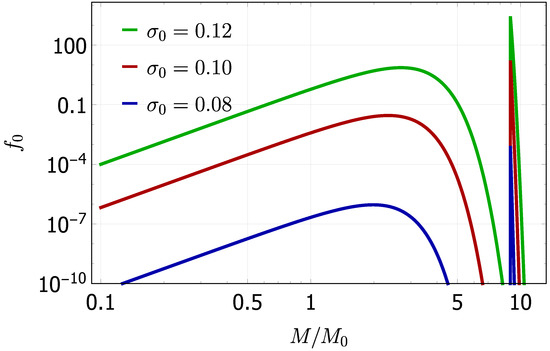
Figure 5. The PBH fractions $f_0$ are plotted as functions of $M/M_0$ for ${\sigma }_0=0.08$, $0.10$ and $0.12$ with $k_0={10}^5{k}_{\mathrm{eq}}$. The right spiky plots show the PBH fractions without the critical behavior, and the left broader plots show those with the critical behavior.

The total fraction $f_{\mathrm{tot}}=\int f_0\mathrm{d}lnM$ is shown as functions of ${\sigma }_0$ for the cases with and without critical behavior in Figure 6.

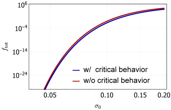
Figure 6. The total fraction $f_{\mathrm{tot}}$ as a function of ${\sigma }_0$.

6. Summary and Further Related Topics

In this review, we have run through the basic picture of PBH formation, cosmological long-wavelength solutions, PBH formation criterion and estimation of PBH abundance in peak theory. In this last section, let us summarize and make notes on each topic.

First, in Section 2, we have considered the three-zone model. It should be noted that the three-zone model cannot be an exact solution for the Einstein field equations with non-vanishing pressure of the fluid, and just gives us intuition about the PBH formation process. Nevertheless, it is interesting that the three-zone model provides us a quantitative threshold value which is roughly equal to the lower bound of the threshold value of the density perturbation [35]. Similar ideas to the three-zone model would be very useful as a foothold when we extend our focus to PBH formations in other settings.

For more accurate analyses, the cosmological long-wavelength solutions are needed to be considered. In Section 3, we just quoted the equations and solutions from Refs. [28,34]. Readers can refer to Refs. [28,34] for more general and concrete derivations and discussions. We note that in Section 3, we have not assumed spherical symmetry. In this sense, the formulation given in Section 3 is more general than the gradient expansion in the Misner–Sharp formulation (e.g., Ref. [72]) which is widely used to construct the initial data for numerical simulations. When one considers other matter components than the perfect fluid with the linear equation of state $p=w\rho$, the cosmological long-wavelength solution should be reconsidered. For example, in Ref. [88], cosmological long-wavelength solutions for massless scalar isocurvature modes have been investigated.

In Section 4, assuming spherical symmetry, we have considered the criterion of PBH formation. Although we need numerical simulations for an accurate criterion, some of the approximate analytic criteria are still practically useful. As a useful and relatively simple criterion, we have introduced the criterion based on the compaction function. The definition of the compaction function is carefully introduced in Section 4 because we recently found a misunderstanding that has not been realized for a long time. More concrete discussions will be reported elsewhere. Since the compaction function is closely related to the conserved mass in a spherically symmetric spacetime, we have provided a short review of the conserved mass and horizons in spherically symmetric spacetimes in Appendix A.

One of the goals of the theoretical PBH study is the estimation of PBH abundance. Since PBHs would be associated with rarely high peaks of a perturbation variable, the peak statistics are relevant to be used. We have attached a short minimal review of the peak theory in Appendix B and Appendix C. We have explained the abundance estimation following Refs. [66,67] mainly focusing on the case of the monochromatic curvature power spectrum. However, different procedures based on peak theory have been also proposed [86,89,90,91]. Here we note that, while the variation of the peak curvature scale is treated as an independent statistical variable in Refs. [66,67,89], the typical profile for the mean peak curvature is only considered in Refs. [86,90]. We may expect that those different procedures predict similar PBH mass spectra for a narrow curvature power spectrum. However, the predictions may be different from each other for a broad curvature power spectrum. This issue is still open and a direct comparison between those different procedures is needed to make a deeper understanding and a consensus.

There are still many interesting open issues we could not mention here such as effects of non-Gaussianity [78,79,80,83,87,92,93,94,95,96,97,98,99,100,101,102,103,104,105,106] PBH in matter dominated era [107,108,109,110,111], non-spherical PBH formation [112], distribution of PBH spin [110,113,114,115,116,117,118], PBH formation in the QCD phase transition epoch [42,80,119,120,121,122,123,124,125,126,127,128,129] and PBH from iso-curvature perturbations [88,130], and so on. PBH formation in modified gravity theories would require more careful treatments in all aspects. We hope this review will be helpful for researchers to study those issues in the future.

References

- Zel’dovich, Y.B.; Novikov, I.D. The Hypothesis of Cores Retarded during Expansion and the Hot Cosmological Model. Soviet Ast. 1967, 10, 602. [Google Scholar]
- Hawking, S. Gravitationally collapsed objects of very low mass. Mon. Not. R. Astron. Soc. 1971, 152, 75–78. [Google Scholar] [CrossRef]
- Carr, B.J.; Hawking, S. Black holes in the early Universe. Mon. Not. R. Astron. Soc. 1974, 168, 399–415. [Google Scholar] [CrossRef]
- Carr, B.J.; Kohri, K.; Sendouda, Y.; Yokoyama, J. New cosmological constraints on primordial black holes. Phys. Rev. D 2010, 81, 104019. [Google Scholar] [CrossRef]
- Carr, B.; Kohri, K.; Sendouda, Y.; Yokoyama, J. Constraints on Primordial Black Holes. arXiv 2020, arXiv:2002.12778. [Google Scholar] [CrossRef]
- Carr, B.; Kuhnel, F. Primordial Black Holes as Dark Matter: Recent Developments. arXiv 2020, arXiv:2006.02838. [Google Scholar] [CrossRef]
- Bird, S.; Cholis, I.; Muñoz, J.B.; Ali-Haïmoud, Y.; Kamionkowski, M.; Kovetz, E.D.; Raccanelli, A.; Riess, A.G. Did LIGO detect dark matter? Phys. Rev. Lett. 2016, 116, 201301. [Google Scholar] [CrossRef]
- Sasaki, M.; Suyama, T.; Tanaka, T.; Yokoyama, S. Primordial Black Hole Scenario for the Gravitational-Wave Event GW150914. Phys. Rev. Lett. 2016, 117, 061101. [Google Scholar] [CrossRef]
- Clesse, S.; García-Bellido, J. Seven Hints for Primordial Black Hole Dark Matter. arXiv 2017, arXiv:1711.10458. [Google Scholar]
- Sasaki, M.; Suyama, T.; Tanaka, T.; Yokoyama, S. Primordial black holes-perspectives in gravitational wave astronomy. Class. Quantum Gravity 2018, 35, 063001. [Google Scholar] [CrossRef]
- Niikura, H.; Takada, M.; Yokoyama, S.; Sumi, T.; Masaki, S. Constraints on Earth-mass primordial black holes from OGLE 5-year microlensing events. Phys. Rev. D 2019, 99, 083503. [Google Scholar] [CrossRef]
- Arzoumanian, Z.; Baker, P.T.; Blumer, H.; Bécsy, B.; Brazier, A.; Brook, P.R.; Burke-Spolaor, S.; Chatterjee, S.; Chen, S.; Cordes, J.M.; et al. The NANOGrav 12.5 yr Data Set: Search for an Isotropic Stochastic Gravitational-wave Background. Astrophys. J. Lett. 2020, 905, L34. [Google Scholar] [CrossRef]
- Vaskonen, V.; Veermäe, H. Did NANOGrav see a signal from primordial black hole formation? Phys. Rev. Lett. 2021, 126, 051303. [Google Scholar] [CrossRef] [PubMed]
- De Luca, V.; Franciolini, G.; Riotto, A. NANOGrav Data Hints at Primordial Black Holes as Dark Matter. Phys. Rev. Lett. 2021, 126, 041303. [Google Scholar] [CrossRef] [PubMed]
- Kohri, K.; Terada, T. Solar-Mass Primordial Black Holes Explain NANOGrav Hint of Gravitational Waves. Phys. Lett. B 2021, 813, 136040. [Google Scholar] [CrossRef]
- Sugiyama, S.; Takhistov, V.; Vitagliano, E.; Kusenko, A.; Sasaki, M.; Takada, M. Testing Stochastic Gravitational Wave Signals from Primordial Black Holes with Optical Telescopes. Phys. Lett. B 2021, 814, 136097. [Google Scholar] [CrossRef]
- Domènech, G.; Pi, S. NANOGrav hints on planet-mass primordial black holes. Sci. China Phys. Mech. Astron. 2022, 65, 230411. [Google Scholar] [CrossRef]
- Inomata, K.; Kawasaki, M.; Mukaida, K.; Yanagida, T. NANOGrav Results and LIGO-Virgo Primordial Black Holes in Axionlike Curvaton Models. Phys. Rev. Lett. 2021, 126, 131301. [Google Scholar] [CrossRef]
- Kawasaki, M.; Kusenko, A.; Yanagida, T. Primordial seeds of supermassive black holes. Phys. Lett. B 2012, 711, 1–5. [Google Scholar] [CrossRef]
- Kohri, K.; Nakama, T.; Suyama, T. Testing scenarios of primordial black holes being the seeds of supermassive black holes by ultracompact minihalos and CMB μ-distortions. Phys. Rev. D 2014, 90, 083514. [Google Scholar] [CrossRef]
- Nakama, T.; Suyama, T.; Yokoyama, J. Supermassive black holes formed by direct collapse of inflationary perturbations. Phys. Rev. D 2016, 94, 103522. [Google Scholar] [CrossRef]
- Carr, B.; Silk, J. Primordial Black Holes as Generators of Cosmic Structures. Mon. Not. R. Astron. Soc. 2018, 478, 3756. [Google Scholar] [CrossRef]
- Serpico, P.D.; Poulin, V.; Inman, D.; Kohri, K. Cosmic microwave background bounds on primordial black holes including dark matter halo accretion. Phys. Rev. Res. 2020, 2, 023204. [Google Scholar] [CrossRef]
- Ünal, C.; Kovetz, E.D.; Patil, S. Multimessenger probes of inflationary fluctuations and primordial black holes. Phys. Rev. D 2021, 103, 063519. [Google Scholar] [CrossRef]
- Kohri, K.; Sekiguchi, T.; Wang, S. Cosmological 21-cm line observations to test scenarios of super-Eddington accretion on to black holes being seeds of high-redshifted supermassive black holes. Phys. Rev. D 2022, 106, 043539. [Google Scholar] [CrossRef]
- Niemeyer, J.C.; Jedamzik, K. Near-critical gravitational collapse and the initial mass function of primordial black holes. Phys. Rev. Lett. 1998, 80, 5481. [Google Scholar] [CrossRef]
- Niemeyer, J.C.; Jedamzik, K. Dynamics of primordial black hole formation. Phys. Rev. D 1999, 59, 124013. [Google Scholar] [CrossRef]
- Shibata, M.; Sasaki, M. Black hole formation in the Friedmann universe: Formulation and computation in numerical relativity. Phys. Rev. D 1999, 60, 084002. [Google Scholar] [CrossRef]
- Hawke, I.; Stewart, J. The dynamics of primordial black-hole formation. Class. Quantum Gravity 2002, 19, 3687. [Google Scholar] [CrossRef]
- Musco, I.; Miller, J.C.; Rezzolla, L. Computations of primordial black hole formation. Class. Quantum Gravity 2005, 22, 1405. [Google Scholar] [CrossRef]
- Harada, T.; Yoo, C.-M.; Kohri, K. Threshold of primordial black hole formation. Phys. Rev. 2013, D88, 084051, Erratum in Phys. Rev. 2014, D89, 029903. [Google Scholar] [CrossRef]
- Nakama, T.; Harada, T.; Polnarev, A.G.; Yokoyama, J. Identifying the most crucial parameters of the initial curvature profile for primordial black hole formation. JCAP 2014, 1401, 037. [Google Scholar] [CrossRef]
- Nakama, T. The double formation of primordial black holes. JCAP 2014, 1410, 040. [Google Scholar] [CrossRef]
- Harada, T.; Yoo, C.-M.; Nakama, T.; Koga, Y. Cosmological long-wavelength solutions and primordial black hole formation. Phys. Rev. D 2015, 91, 084057. [Google Scholar] [CrossRef]
- Musco, I. Threshold for primordial black holes: Dependence on the shape of the cosmological perturbations. Phys. Rev. D 2019, 100, 123524. [Google Scholar] [CrossRef]
- Escrivà, A. Simulation of primordial black hole formation using pseudo-spectral methods. Phys. Dark Univ. 2020, 27, 100466. [Google Scholar] [CrossRef]
- Escrivà, A.; Germani, C.; Sheth, R. Universal threshold for primordial black hole formation. Phys. Rev. D 2020, 101, 044022. [Google Scholar] [CrossRef]
- Escrivà, A.; Germani, C.; Sheth, R.K. Analytical thresholds for black hole formation in general cosmological backgrounds. arXiv 2020, arXiv:2007.05564. [Google Scholar] [CrossRef]
- Escrivà, A. PBH Formation from Spherically Symmetric Hydrodynamical Perturbations: A Review. Universe 2022, 8, 66. [Google Scholar] [CrossRef]
- Musco, I.; Papanikolaou, T. Primordial black hole formation for an anisotropic perfect fluid: Initial conditions and estimation of the threshold. Phys. Rev. D 2022, 106, 083017. [Google Scholar] [CrossRef]
- Escrivà, A.; Bagui, E.; Clesse, S. Simulations of PBH formation at the QCD epoch and comparison with the GWTC-3 catalog. arXiv 2022, arXiv:2209.06196. [Google Scholar]
- Franciolini, G.; Musco, I.; Pani, P.; Urbano, A. From inflation to black hole mergers and back again: Gravitational-wave data-driven constraints on inflationary scenarios with a first-principle model of primordial black holes across the QCD epoch. arXiv 2022, arXiv:2209.05959. [Google Scholar]
- Papanikolaou, T. Toward the primordial black hole formation threshold in a time-dependent equation-of-state background. Phys. Rev. D 2022, 105, 124055. [Google Scholar] [CrossRef]
- Toussaint, D.; Treiman, S.B.; Wilczek, F.; Zee, A. Matter-antimatter accounting, thermodynamics, and black-hole radiation. Phys. Rev. D 1979, 19, 1036. [Google Scholar] [CrossRef]
- Barrow, J.D.; Copeland, E.; Kolb, E.; Liddle, A.R. Baryogenesis in extended inflation. 2. Baryogenesis via primordial black holes. Phys. Rev. D 1991, 43, 984. [Google Scholar] [CrossRef] [PubMed]
- Baumann, D.; Steinhardt, P.J.; Turok, N. Primordial Black Hole Baryogenesis. arXiv 2007, arXiv:hep-th/0703250. [Google Scholar]
- Inomata, K.; Kawasaki, M.; Mukaida, K.; Terada, T.; Yanagida, T.T. Gravitational Wave Production right after a Primordial Black Hole Evaporation. Phys. Rev. D 2020, 101, 123533. [Google Scholar] [CrossRef]
- Papanikolaou, T.; Vennin, V.; Langlois, D. Gravitational waves from a universe filled with primordial black holes. JCAP 2021, 053. [Google Scholar] [CrossRef]
- Domènech, G.; Lin, C.; Sasaki, M. Gravitational wave constraints on the primordial black hole dominated early universe. JCAP 2021, 062, Erratum in JCAP 2021, 11, E01. [Google Scholar] [CrossRef]
- Bhaumik, N.; Jain, R.K. Small scale induced gravitational waves from primordial black holes, a stringent lower mass bound, and the imprints of an early matter to radiation transition. Phys. Rev. D 2021, 104, 023531. [Google Scholar] [CrossRef]
- Hooper, D.; Krnjaic, G.; March-Russell, J.; McDermott, S.D.; Petrossian-Byrne, R. Hot Gravitons and Gravitational Waves From Kerr Black Holes in the Early Universe. arXiv 2020, arXiv:2004.00618. [Google Scholar]
- Domènech, G.; Takhistov, V.; Sasaki, M. Exploring evaporating primordial black holes with gravitational waves. Phys. Lett. B. 2021, 823, 136722. [Google Scholar] [CrossRef]
- Ananda, K.N.; Clarkson, C.; Wands, D. The Cosmological gravitational wave background from primordial density perturbations. Phys. Rev. D 2007, 75, 123518. [Google Scholar] [CrossRef]
- Baumann, D.; Steinhardt, P.J.; Takahashi, K.; Ichiki, K. Gravitational Wave Spectrum Induced by Primordial Scalar Perturbations. Phys. Rev. D 2007, 76, 084019. [Google Scholar] [CrossRef]
- Saito, R.; Yokoyama, J. Gravitational wave background as a probe of the primordial black hole abundance. Phys. Rev. Lett. 2009, 102, 161101, Erratum in Phys. Rev. Lett. 2011, 107, 069901. [Google Scholar] [CrossRef]
- Saito, R.; Yokoyama, J. Gravitational-Wave Constraints on the Abundance of Primordial Black Holes. Prog. Theor. Phys. 2010, 123, 867, Erratum in Prog. Theor. Phys. 2011, 126, 351–352. [Google Scholar] [CrossRef]
- Assadullahi, H.; Wands, D. Gravitational waves from an early matter era. Phys. Rev. D 2009, 79, 083511. [Google Scholar] [CrossRef]
- Bugaev, E.; Klimai, P. Induced gravitational wave background and primordial black holes. Phys. Rev. D. 2010, 81, 023517. [Google Scholar] [CrossRef]
- Bugaev, E.; Klimai, P. Constraints on the induced gravitational wave background from primordial black holes. Phys. Rev. D. 2011, 83, 083521. [Google Scholar] [CrossRef]
- Espinosa, J.R.; Racco, D.; Riotto, A. A Cosmological Signature of the SM Higgs Instability: Gravitational Waves. JCAP 2018, 012. [Google Scholar] [CrossRef]
- Kohri, K.; Terada, T. Semianalytic calculation of gravitational wave spectrum nonlinearly induced from primordial curvature perturbations. Phys. Rev. D 2018, 97, 123532. [Google Scholar] [CrossRef]
- Domènech, G. Scalar Induced Gravitational Waves Review. Universe 2021, 7, 398. [Google Scholar] [CrossRef]
- Escrivà, A.; Kuhnel, F.; Tada, Y. Primordial Black Holes. arXiv 2022, arXiv:2211.05767. [Google Scholar]
- Villanueva-Domingo, P.; Mena, O.; Palomares-Ruiz, S. A brief review on primordial black holes as dark matter. Front. Astron. Space Sci. 2021, 8, 87. [Google Scholar] [CrossRef]
- Byrnes, C.T.; Cole, P.S. Lecture notes on inflation and primordial black holes. arXiv 2021, arXiv:2112.05716. [Google Scholar]
- Yoo, C.-M.; Harada, T.; Garriga, J.; Kohri, K. Primordial black hole abundance from random Gaussian curvature perturbations and a local density threshold. PTEP 2018, 2018, 123E01. [Google Scholar] [CrossRef]
- Yoo, C.-M.; Harada, T.; Hirano, S.; Kohri, K. Abundance of Primordial Black Holes in Peak Theory for an Arbitrary Power Spectrum. arXiv 2020, arXiv:2008.02425. [Google Scholar] [CrossRef]
- Bardeen, J.M.; Bond, J.R.; Kaiser, N.; Szalay, A.S. The statistics of peaks of Gaussian random fields. Astrophys. J. 1986, 304, 15. [Google Scholar] [CrossRef]
- Kopp, M.; Hofmann, S.; Weller, J. Separate Universes Do Not Constrain Primordial Black Hole Formation. Phys. Rev. 2011, D83, 124025. [Google Scholar] [CrossRef]
- Carr, B.J. The Primordial black hole mass spectrum. Astrophys. J. 1975, 201, 1. [Google Scholar] [CrossRef]
- Misner, C.W.; Sharp, D.H. Relativistic equations for adiabatic, spherically symmetric gravitational collapse. Phys. Rev. 1964, 136, B571. [Google Scholar] [CrossRef]
- Polnarev, A.G.; Musco, I. Curvature profiles as initial conditions for primordial black hole formation. Class. Quantum Gravity 2007, 24, 1405. [Google Scholar] [CrossRef]
- Lyth, D.H.; Malik, K.A.; Sasaki, M. A General proof of the conservation of the curvature perturbation. JCAP 2005, 004. [Google Scholar] [CrossRef]
- Nadezhin, D.K.; Novikov, I.D.; Polnarev, A.G. The hydrodynamics of primordial black hole formation. Soviet Ast. 1978, 22, 129. [Google Scholar]
- Novikov, I.D.; Polnarev, A.G. The Hydrodynamics of Primordial Black Hole Formation—Dependence on the Equation of State. Soviet Ast. 1980, 24, 147. [Google Scholar]
- Musco, I.; Miller, J.C.; Polnarev, A.G. Primordial black hole formation in the radiative era: Investigation of the critical nature of the collapse. Class. Quantum Gravity 2009, 26, 235001. [Google Scholar] [CrossRef]
- Musco, I.; Miller, J.C. Primordial black hole formation in the early universe: Critical behaviour and self-similarity. Class. Quantum Gravity 2013, 30, 145009. [Google Scholar] [CrossRef]
- Yoo, C.-M.; Gong, J.-O.; Yokoyama, S. Abundance of primordial black holes with local non-Gaussianity in peak theory. JCAP 2019, 033. [Google Scholar] [CrossRef]
- Kitajima, N.; Tada, Y.; Yokoyama, S.; Yoo, C.-M. Primordial black holes in peak theory with a non-Gaussian tail. JCAP 2021, 10, 053. [Google Scholar] [CrossRef]
- Escrivà, A.; Tada, Y.; Yokoyama, S.; Yoo, C.-M. Simulation of primordial black holes with large negative non-Gaussianity. JCAP 2022, 5, 012. [Google Scholar] [CrossRef]
- Choptuik, M.W. Universality and scaling in gravitational collapse of a massless scalar field. Phys. Rev. Lett. 1993, 70, 9. [Google Scholar] [CrossRef] [PubMed]
- Koike, T.; Hara, T.; Adachi, S. Critical behavior in gravitational collapse of radiation fluid: A Renormalization group (linear perturbation) analysis. Phys. Rev. Lett. 1995, 74, 5170. [Google Scholar] [CrossRef] [PubMed]
- Yokoyama, J. Cosmological constraints on primordial black holes produced in the near critical gravitational collapse. Phys. Rev. D 1998, 58, 107502. [Google Scholar] [CrossRef]
- Green, A.M.; Liddle, A.R. Critical collapse and the primordial black hole initial mass function. Phys. Rev. D 1999, 60, 063509. [Google Scholar] [CrossRef]
- Kuhnel, F.; Rampf, C.; Sandstad, M. Effects of Critical Collapse on Primordial Black-Hole Mass Spectra. Eur. Phys. J. C 2016, 76, 93. [Google Scholar] [CrossRef]
- Germani, C.; Musco, I. Abundance of Primordial Black Holes Depends on the Shape of the Inflationary Power Spectrum. Phys. Rev. Lett. 2019, 122, 141302. [Google Scholar] [CrossRef]
- Biagetti, M.; DeLuca, V.; Franciolini, G.; Kehagias, A.; Riotto, A. The formation probability of primordial black holes. Phys. Lett. B 2021, 820, 136602. [Google Scholar] [CrossRef]
- Yoo, C.-M.; Harada, T.; Hirano, S.; Okawa, H.; Sasaki, M. Primordial black hole formation from massless scalar isocurvature. Phys. Rev. D 2022, 105, 103538. [Google Scholar] [CrossRef]
- Germani, C.; Sheth, R.K. Nonlinear statistics of primordial black holes from Gaussian curvature perturbations. Phys. Rev. D 2020, 101, 063520. [Google Scholar] [CrossRef]
- Musco, I.; DeLuca, V.; Franciolini, G.; Riotto, A. Threshold for primordial black holes. II. A simple analytic prescription. Phys. Rev. D 2021, 103, 063538. [Google Scholar] [CrossRef]
- Suyama, T.; Yokoyama, S. A novel formulation of the PBH mass function. PTEP 2020, 2020, 023E03. [Google Scholar]
- Bullock, J.S.; Primack, J.R. NonGaussian fluctuations and primordial black holes from inflation. Phys. Rev. D 1997, 55, 7423. [Google Scholar] [CrossRef]
- Ivanov, P. Nonlinear metric perturbations and production of primordial black holes. Phys. Rev. D 1998, 57, 7145. [Google Scholar] [CrossRef]
- Hidalgo, J.C. The effect of non-Gaussian curvature perturbations on the formation of primordial black holes. arXiv 2007, arXiv:0708.3875. [Google Scholar]
- Byrnes, C.T.; Copeland, E.J.; Green, A.M. Primordial black holes as a tool for constraining non-Gaussianity. Phys. Rev. D 2012, 86, 043512. [Google Scholar] [CrossRef]
- Bugaev, E.V.; Klimai, P.A. Primordial black hole constraints for curvaton models with predicted large non-Gaussianity. Int. J. Mod. Phys. D 2013, 22, 1350034. [Google Scholar] [CrossRef]
- Young, S.; Regan, D.; Byrnes, C.T. Influence of large local and non-local bispectra on primordial black hole abundance. JCAP 2016, 2, 029. [Google Scholar] [CrossRef][Green Version]
- Nakama, T.; Silk, J.; Kamionkowski, M. Stochastic gravitational waves associated with the formation of primordial black holes. Phys. Rev. D 2017, 95, 043511. [Google Scholar] [CrossRef]
- Ando, K.; Inomata, K.; Kawasaki, M.; Mukaida, K.; Yanagida, T.T. Primordial black holes for the LIGO events in the axionlike curvaton model. Phys. Rev. D 2018, 97, 123512. [Google Scholar] [CrossRef]
- Franciolini, G.; Kehagias, A.; Matarrese, S.; Riotto, A. Primordial Black Holes from Inflation and non-Gaussianity. JCAP 2018, 1803, 016. [Google Scholar] [CrossRef]
- Cai, R.-g.; Pi, S.; Sasaki, M. Gravitational Waves Induced by non-Gaussian Scalar Perturbations. Phys. Rev. Lett. 2019, 122, 201101. [Google Scholar] [CrossRef] [PubMed]
- Atal, V.; Germani, C. The role of non-gaussianities in Primordial Black Hole formation. Phys. Dark Univ. 2019, 24, 100275. [Google Scholar] [CrossRef]
- Passaglia, S.; Hu, W.; Motohashi, H. Primordial black holes and local non-Gaussianity in canonical inflation. Phys. Rev. D 2019, 99, 043536. [Google Scholar] [CrossRef]
- Taoso, M.; Urbano, A. Non-gaussianities for primordial black hole formation. JCAP 2021, 8, 016. [Google Scholar] [CrossRef]
- Atal, V.; Garriga, J.; Marcos-Caballero, A. Primordial black hole formation with non-Gaussian curvature perturbations. JCAP 2019, 073. [Google Scholar] [CrossRef]
- Atal, V.; Cid, J.; Escrivà, A.; Garriga, J. PBH in single field inflation: The effect of shape dispersion and non-Gaussianities. JCAP 2020, 022. [Google Scholar] [CrossRef]
- Khlopov, M.Y.; Polnarev, A.G. Primordial black holes as a cosmological test of grand unification. Phys. Lett. 1980, 97B, 383. [Google Scholar] [CrossRef]
- Polnarev, A.G.; Khlopov, M.Y. Cosmology, primordial black holes, and supermassive particles. Sov. Phys. Usp. 1985, 28, 213. [Google Scholar] [CrossRef]
- Harada, T.; Yoo, C.-M.; Kohri, K.; Nakao, K.-i.; Jhingan, S. Primordial black hole formation in the matter-dominated phase of the Universe. Astrophys. J. 2016, 833, 61. [Google Scholar] [CrossRef]
- Harada, T.; Yoo, C.-M.; Kohri, K.; Nakao, K.-I. Spins of primordial black holes formed in the matter-dominated phase of the Universe. arXiv 2017, arXiv:1707.03595. [Google Scholar] [CrossRef]
- Kokubu, T.; Kyutoku, K.; Kohri, K.; Harada, T. Effect of Inhomogeneity on Primordial Black Hole Formation in the Matter Dominated Era. Phys. Rev. D 2018, 98, 123024. [Google Scholar] [CrossRef]
- Yoo, C.-M.; Harada, T.; Okawa, H. Threshold of Primordial Black Hole Formation in Nonspherical Collapse. arXiv 2020, arXiv:2004.01042. [Google Scholar] [CrossRef]
- Chiba, T.; Yokoyama, S. Spin Distribution of Primordial Black Holes. PTEP 2017, 2017, 083E01. [Google Scholar] [CrossRef]
- DeLuca, V.; Franciolini, G.; Pani, P.; Riotto, A. The evolution of primordial black holes and their final observable spins. JCAP 2020, 052. [Google Scholar] [CrossRef]
- Mirbabayi, M.; Gruzinov, A.; Noreña, J. Spin of Primordial Black Holes. JCAP 2020, 017. [Google Scholar] [CrossRef]
- He, M.; Suyama, T. Formation threshold of rotating primordial black holes. Phys. Rev. D 2019, 100, 063520. [Google Scholar] [CrossRef]
- Flores, M.M.; Kusenko, A. Spins of primordial black holes formed in different cosmological scenarios. Phys. Rev. D 2021, 104, 063008. [Google Scholar] [CrossRef]
- Koga, Y.; Harada, T.; Tada, Y.; Yokoyama, S.; Yoo, C.-M. Effective inspiral spin distribution of primordial black hole binaries. arXiv 2022, arXiv:2208.00696. [Google Scholar] [CrossRef]
- Jedamzik, K. Primordial black hole formation during the QCD epoch. Phys. Rev. D 1997, 55, 5871. [Google Scholar] [CrossRef]
- Schmid, C.; Schwarz, D.J.; Widerin, P. Amplification of cosmological inhomogeneities from the QCD transition. Phys. Rev. D 1999, 59, 043517. [Google Scholar] [CrossRef]
- Widerin, P.; Schmid, C. Primordial black holes from the QCD transition? arXiv 1998, arXiv:astro-ph/9808142. [Google Scholar]
- Boeckel, T.; Schettler, S.; Schaffner-Bielich, J. The Cosmological QCD Phase Transition Revisited. Prog. Part. Nucl. Phys. 2011, 66, 266. [Google Scholar] [CrossRef]
- Sobrinho, J.L.G.; Augusto, P.; Gonçalves, A.L. New thresholds for Primordial Black Hole formation during the QCD phase transition. Mon. Not. Roy. Astron. Soc. 2016, 463, 2348. [Google Scholar] [CrossRef]
- Byrnes, C.T.; Hindmarsh, M.; Young, S.; Hawkins, M.R.S. Primordial black holes with an accurate QCD equation of state. JCAP 2018, 041. [Google Scholar] [CrossRef]
- Carr, B.; Clesse, S.; García-Bellido, J.; Kühnel, F. Cosmic conundra explained by thermal history and primordial black holes. Phys. Dark Univ. 2021, 31, 100755. [Google Scholar] [CrossRef]
- Carr, B.; Clesse, S.; García-Bellido, J. Primordial black holes from the QCD epoch: Linking dark matter, baryogenesis and anthropic selection. Mon. Not. R. Astron. Soc. 2021, 501, 1426. [Google Scholar] [CrossRef]
- Clesse, S.; Garcia-Bellido, J. GW190425, GW190521 and GW190814: Three candidate mergers of primordial black holes from the QCD epoch. arXiv 2020, arXiv:2007.06481. [Google Scholar] [CrossRef]
- Gao, F.; Oldengott, I.M. Cosmology Meets Functional QCD: First-Order Cosmic QCD Transition Induced by Large Lepton Asymmetries. Phys. Rev. Lett. 2022, 128, 131301. [Google Scholar] [CrossRef]
- Juan, J.I.; Serpico, P.D.; FrancoAbellán, G. The QCD phase transition behind a PBH origin of LIGO/Virgo events? JCAP 2022, 009. [Google Scholar] [CrossRef]
- Passaglia, S.; Sasaki, M. Primordial Black Holes from CDM Isocurvature. arXiv 2021, arXiv:2109.12824. [Google Scholar]
- Kodama, H. Conserved Energy Flux for the Spherically Symmetric System and the Back Reaction Problem in the Black Hole Evaporation. Prog. Theor. Phys. 1980, 63, 1217. [Google Scholar] [CrossRef]
- Hayward, S.A. General laws of black hole dynamics. Phys. Rev. D 1994, 49, 6467. [Google Scholar] [CrossRef] [PubMed]
- Hayward, S.A. Gravitational energy in spherical symmetry. Phys. Rev. D 1996, 53, 1938. [Google Scholar] [CrossRef] [PubMed]
Publisher’s Note: MDPI stays neutral with regard to jurisdictional claims in published maps and institutional affiliations. |
© 2022 by the author. Licensee MDPI, Basel, Switzerland. This article is an open access article distributed under the terms and conditions of the Creative Commons Attribution (CC BY) license (https://creativecommons.org/licenses/by/4.0/).