A Framework for Anomaly Detection and Evaluation of Rotating Machinery Based on Data-Accumulation-Aware Generative Adversarial Networks and Similarity Estimation

Abstract

Rotating machinery plays a critical role in industrial systems, and effective anomaly detection and assessment are indispensable for ensuring operational safety and reliability. However, the performance of existing methods is often constrained by the difficulty in acquiring fault samples—such samples are typically scarce during the initial operational phase of equipment. To address this challenge, this paper proposes a novel anomaly detection and evaluation framework based on Data-Accumulation-Aware Generative Adversarial Networks (DAA-GANs) and similarity estimation. The core innovation of this framework lies in its adaptability across different data accumulation stages. During the early operational phase dominated by normal samples, only normal data is used to train the DAA-GAN to establish a baseline detector. As fault data gradually accumulates, the detection threshold undergoes adaptive adjustment through collaborative optimization of normal and abnormal samples, thereby enhancing the detector’s generalization capability. Upon amassing annotated fault samples of varying severity, the framework assesses anomaly severity by analyzing the similarity between test outputs of unknown samples and known fault samples. The framework is validated through two case studies: a fault simulation model for a torque-splitting transmission system and the publicly available Case Western Reserve University (CWRU) bearing dataset. In the simulation case, the detection accuracy reaches 100% for the gear tooth breakage levels. On the CWRU dataset, the proposed method achieves an overall average detection accuracy of 99.83% across three operating speeds (1730/1750/1772 rpm), and the similarity-based assessment provides consistent severity identification. These results demonstrate that the proposed framework can support reliable anomaly detection and severity assessments under progressive data accumulation.

1. Introduction

In modern large-scale industrial installations such as machinery and power plants, rotating machinery constitutes an indispensable universal component within mechanical equipment. The success of industrial enterprises likewise hinges upon the secure operation of their equipment systems. Within mechanical engineering, should mechanical equipment suffer a malfunction, minor faults will diminish the equipment’s operational functionality, directly impacting production; severe faults, however, may precipitate catastrophic incidents. Equipment health monitoring and fault diagnosis constitute vital components of preventive maintenance systems, playing a significant role in extending the operational lifespan of machinery, reducing maintenance costs, and enhancing operational safety.

The operational status of rotating machinery directly influences critical performance parameters of large-scale equipment, including machining precision, operational reliability, and service life. Research into health monitoring, fault diagnosis, and predictive methodologies for rotating machinery forms the foundation for ensuring the safe and stable operation of mechanical equipment [1,2]. In recent years, deep learning has achieved remarkable success in numerous data prediction and classification tasks. Leveraging extensive historical data stored within systems and operating without requiring precise physical models, data-driven fault diagnosis methods have gained widespread application in intelligent factories and the health monitoring and fault diagnosis of mechanical equipment [3].

Deep learning has become an effective paradigm for feature extraction, alleviating the limitations of shallow learning in capturing highly nonlinear patterns from large-scale data. Nevertheless, the robust performance of deep learning-based fault diagnosis still hinges on the availability of sufficient, high-quality training data. In rotating machinery, fault events (e.g., catastrophic failures or abrupt malfunctions) are typically scarce, whereas normal-condition data are abundant [4], making class imbalance a pervasive challenge. To mitigate this issue, Viola et al [5] employed time–frequency transformations to obtain two-dimensional representations of vibration signals and used deep convolutional GANs to generate both normal and faulty samples. Zhou et al [6] proposed a globally optimized generative adversarial network to learn fault-feature generation under imbalanced conditions. Xie and Zhang [7] introduced a deep convolutional generative adversarial network (DCGAN) to address sample imbalance; after balancing the dataset via DCGAN-based sample generation, statistical features from time-domain and frequency-domain signals were extracted to train an SVM classifier for bearing fault classification, showing improved performance over conventional resampling strategies (e.g., random oversampling/undersampling and synthetic undersampling) under highly imbalanced settings. Beyond sample-count imbalance, real industrial datasets often present additional constraints such as heterogeneous sampling rates and limited fault coverage. For example, Huang et al. [8] developed a deep learning model tailored to multirate industrial measurements and reported that reliable diagnosis can still be achieved under severe imbalance in practice. Zareapoor et al. [9] further proposed an oversampling adversarial network that explicitly generates minority-class samples to enhance diagnosis performance for class-imbalanced conditions. In another industrial application, Yan et al. [10] combined a VAE with adversarial generation to synthesize informative fault patterns for chiller fault diagnosis when fault data are limited. However, most data-augmentation-oriented solutions still assume the presence of at least a small number of fault samples for model calibration and validation. In practical deployments—especially during early-life or newly commissioned stages—fault data may be entirely unavailable, which motivates lifecycle-aware methods that can perform stable and accurate detection under extreme imbalance (including normal-only training) and progressively adapt as fault data accumulate.

Recent studies have emphasized robustness under variable working conditions and model interpretability. For instance, Spirto et al. [11] proposed a VKF-MOT-SDP-CNN pipeline to enhance gear fault detection under variable operating conditions, and Chen et al. [12] developed an interpretable wavelet Kolmogorov–Arnold Convolutional LSTM for spatio-temporal feature extraction and intelligent fault diagnosis. These advances further motivate the development of lifecycle-aware and explainable anomaly detection frameworks for rotating machinery.

Anomaly detection (AD), also known as outlier detection (OD) or novelty detection (ND), refers to the identification of data points that deviate significantly from the majority of the dataset [13]. Consequently, anomaly detection can address more extreme instances of data imbalance.

Currently, mechanical equipment anomaly detection methods are primarily categorized into three types: boundary-based approaches, probability density estimation-based approaches, and deep learning-based approaches [14]. Boundary-based anomaly detection methods establish boundaries for training datasets to determine the classification of unknown objects, thereby enabling anomaly detection. The core principle of probability density estimation-based anomaly detection is that outliers can be identified in low-density regions, whereas normal values reside in high-density regions.

Maliuk, A.S. et al. [15] proposed a bearing fault detection method based on Gaussian Mixture Models (GMM). This approach utilizes GMM window sequences oriented towards fault frequencies for signal feature extraction, employing a weighted K-nearest neighbor algorithm for fault classification. The aforementioned approaches separate feature extraction from model construction. Numerous classical methods exist for feature extraction, including time-frequency feature extraction [16], wavelet decomposition [17], and empirical mode decomposition [18]. With advances in modern industrial technology, the widespread application of various sensors has led to a substantial increase in data volumes for detection objects. Traditional methods struggle to identify outliers within large datasets [19], whereas deep learning has demonstrated excellent performance in handling big data [20]. Zhang et al. [21] employed a deep generative model based on Variational Autoencoders (VAE) for bearing anomaly detection, effectively leveraging sparse labeled information within datasets with favorable outcomes. Lee et al. [22] utilized stacked Convolutional Neural Networks (CNNs) to extract features from vibration sensor signal patterns, then trained a stacked bidirectional Long Short-Term Memory (LSTM) network on these features, ultimately achieving anomaly prediction through a regression layer. Ahmad et al. [23] proposed an autoencoder-based method for rotating machinery condition monitoring, directly extracting features from raw vibration signals without manual feature design. Experimental results demonstrated superior performance compared to manually engineered features.

Generative adversarial network (GAN) models have garnered increasing attention from researchers in recent years. First proposed by Goodfellow et al. [24], they were initially applied to image generation. Given a deterministic dataset, GAN models learn to generate new data that share the same statistical distribution as the original dataset. To address anomaly detection requirements for fault-free data, Schlegl et al. [25] introduced the first GAN framework for anomaly detection, AnoGAN. Donahue et al. [26] introduced the BiGAN architecture to anomaly detection, aiming to overcome limitations of AnoGAN. GANomaly [27] enhanced the loss function to improve model stability. Ou et al. [12] leveraged the memory properties of LSTM networks and GAN models to achieve robust results in bearing signal anomaly detection across varying signal-to-noise ratios. Jiang et al. [28] trained a triple encoder–decoder-encoder network generator to learn features meticulously extracted from normal samples. Hu et al. [29] proposed a Wasserstein Generative Digital Twin (WGDT) model capable of stably and efficiently simulating the distribution of healthy physical samples, ensuring high fidelity between virtually generated and physical samples.

Although GANs have achieved preliminary breakthroughs in anomaly detection, model training is prone to collapse, and detection accuracy remains insufficient for identifying anomalies across different device stages. Consequently, it is imperative to design distinct detection and evaluation methodologies tailored to various operational phases of equipment. Such frameworks should enable health monitoring during early stages without reliance on fault data, leverage mature monitoring models during intermediate and late stages, and facilitate assessment of anomaly severity.

Inspired by the aforementioned research, this paper constructs an anomaly detection and evaluation framework based on Data Accumulation-Aware Generative Adversarial Networks (DAA-GAN). This framework adapts to the varying stages of anomaly data accumulation in equipment, employing distinct detection and evaluation methodologies for each phase. In the first stage, the equipment operates normally with no fault data available. Models are trained solely on normal data to learn its distribution, aligning closely with practical applications. During the second stage, when minor faults emerge and limited anomaly data becomes available, error reduction is achieved by adjusting decision thresholds and evaluation outcomes. In the third stage, with substantial fault data accumulation, the probability distributions of anomaly scores across different fault categories and severity levels are statistically analyzed. Pearson correlation coefficients are calculated to identify and classify faults, while similarity features are employed to assess anomaly severity. Experimental results demonstrate the stability and efficacy of the DAA-GAN approach.

This approach enables phased detection of anomalies in machine operation under conditions of extreme sample data imbalance. Different detection and evaluation methods can be applied according to the stage of accumulated equipment anomaly data. It facilitates health monitoring during the initial phase without any fault data, while leveraging mature detection models to assess anomaly severity in the middle and later stages. Fault diagnosis: Following equipment failure or abnormality detection, the proposed framework can rapidly identify the fault category and assess its severity based on anomaly-score distributions, thereby providing quantitative decision support for maintenance personnel to restore operation. It is worth nothing that determining underlying root causes (e.g., crack initiation mechanisms or specific defect formation causes) typically requires additional physics-based investigation and operational context, which is beyond the scope of this paper and is left for future integration.

Key highlights of this work are as follows:

(1) DAA-GAN enables phased equipment detection, employing distinct detection and evaluation methods according to the accumulation stage of anomaly data. It facilitates health monitoring during the initial phase without fault data, while utilizing mature detection models to assess anomaly severity in the middle and later stages.

(2) The proposed method demonstrates high detection rates for mechanical equipment conditions and effectively distinguishes between fault severity levels. Experimental results confirm our approach maintains stable high performance, ensuring excellent anomaly detection accuracy even under imbalanced data conditions.

(3) The framework was validated using a split-torque transmission system dataset and open datasets, enabling a stepwise approach to anomaly detection, threshold optimization, and optimal assessment.

2. Anomaly Detection and Assessment Framework

This section details the proposed anomaly detection and evaluation framework alongside its Data-Accumulation-Aware Generative Adversarial Network (DAA-GAN) model. Unlike traditional GAN-based approaches such as AnoGAN and GANomaly, which focus solely on single-stage unsupervised anomaly detection, our approach integrates DAA-GAN with the phased evolution of data during device operation. It learns the normal distribution using only healthy samples, performs threshold adaptation optimization upon the emergence of a small number of fault samples, and introduces similarity assessments to determine fault severity as fault samples gradually accumulate. This design better accommodates the characteristics of evolving device states and progressively accumulating data in real-world engineering scenarios.

2.1. Theoretical Background

Generative adversarial networks (GANs) and their variants have been widely adopted for representation learning and anomaly detection. In this work, we build upon the GAN-based anomaly detection paradigm and employ a DAA-GAN model to learn normal-condition representations and produce anomaly scores for input samples. These anomaly scores are subsequently utilized in a staged framework: Stage I performs unsupervised detection using only normal data; Stage II updates the decision threshold when limited labeled faults become available; and Stage III conducts severity assessment by comparing anomaly-score distributions via similarity measures.

For conciseness and readability, the standard GAN objective and the commonly used GANomaly-style background formulation are summarized in Appendix A, while the main text focuses on the proposed staged design and implementation details that are specific to this study.

2.2. A Comprehensive Framework for Anomaly Detection and Estimation

In practice, fault data of rotating machinery are progressively accumulated during the equipment lifecycle: the system starts with only normal data, then a small number of fault samples appear, and finally multiple fault categories and severities are observed. To explicitly reflect this process, this paper proposes a three-stage, da-ta-accumulation-aware framework built upon DAA-GAN. The framework contains three key modules: (i) a DAA-GAN-based anomaly detector trained with only normal samples, (ii) an adaptive threshold update strategy using limited fault samples, and (iii) a multi-index similarity fusion strategy for anomaly severity assessment based on anomaly-score probability density distributions.

Stage I (no-fault stage): only normal data are available. DAA-GAN is trained using normal samples to learn the normal latent patterns and data distribution, providing an unsupervised anomaly detector.

Stage II (few-fault stage): a small amount of fault data becomes available. The decision threshold is updated on a validation set by selecting the threshold that minimizes the total error (FAR+MAR), which improves the robustness of detection under early-fault and imbalanced conditions.

Stage III (many-fault stage): sufficient fault samples with labeled severities are accumulated. The anomaly-score distributions of the test samples are compared with reference fault distributions using multiple similarity measures (KL/JS divergences and correlation coefficients). After directional alignment and normalization, these similarity scores are fused to identify the most similar fault type/severity.

Notably, the proposed DAA-GAN structure focuses on robust unsupervised representation learning for anomaly detection, while the stage-dependent threshold adaptation and similarity fusion strategies enable the framework to operate effectively when fault data evolve from ‘none’ to ‘few’ and to ‘many’. The specific framework diagram is shown in Figure 1 below.

Figure 1. The overall framework.

2.3. Anomaly Detection Based on DAA-GAN

This section proposes a deep learning model based on Data Accumulation-Aware Generative Adversarial Networks (DAA-GAN) for rolling bearing anomaly detection under varying operating conditions and imbalanced datasets. For the generator, two encoders learn representations of the latent features and the regenerated features, respectively, from the raw data. The decoder attempts to simultaneously reconstruct. The entire process is as follows:

DAA-GAN adopts the GANomaly-style encoder–decoder–encoder backbone as the core unsupervised anomaly detector and is integrated into the proposed data-accumulation-aware framework. In this study, the network provides a unified anomaly-score generation mechanism across lifecycle stages, while the stage-dependent strategies (adaptive threshold update and similarity-based assessment) constitute the main extensions that enable practical deployment under progressively accumulated fault data.

(1) $G_e$ is composed of the convolutional layer, the BatchNorm layer, and the leaky ReLU activation layer.

$$Z=G_e(F),Z\in {ℝ}^{h\times b}$$

(1)

$G_e$ reduces the dimension of F to the hidden feature Z, where h is the dimension of the hidden vector Z. b is the number of training samples.

(2) $G_d$ is composed of the convolutional transposition layer, the leaky ReLU activation layer, and the BatchNorm layer. $G_d$ re-decodes Z into $\widehat{F}$.

$$\widehat{F}=G_d(G_e(F))$$

(2)

(3) The last encoder ${\widehat{G}}_e$ has the same structure${ G}_e$ but with different parameters, and the output $\widehat{Z}$ has the same dimension as Z.

$$\widehat{Z}={\widehat{G}}_e(G_d(G_e(F)))$$

(3)

The generator learns both the properties of the original feature set F and the patterns of the latent vector Z simultaneously. Meanwhile, discriminator D employs the standard discriminator network introduced in DCGAN to distinguish between real and generated input data. Once the overall network architecture is defined, the next step is to define the loss function used for training.

During the training phase, only the normal dataset $D_{\mathit{train}}$ is considered, the model $M$ acquires normal patterns exclusively. However, in the testing phase, $M$ one must discern faulty samples by generating higher anomaly scores. This implies that $G_d$ and ${ G}_e$ will decode Z and encode $\widehat{F}$. Consequently, $\widehat{F}$ and $\widehat{Z}$ will inevitably diverge from the original F and Z, aiding in fault identification. Given that this generator utilizes a triple-subnet structure involving encoding, decoding, and encoding, its final loss function comprises three components: fraud loss, apparent loss, and latent loss.

Fraud Loss: Fraud loss $L_f$ is designed to compel the discriminator to misclassify the generated samples from the generator as real samples. The fraud loss is calculated using the output of the discriminator, with the formula as follows:

$$L_f(F)={\displaystyle \sum _{i=1}^N\sigma (C(\widehat{F}),\alpha )}$$

(4)

where $\sigma$ is the binary cross-entropy loss function and $C\left(\widehat{F}\right)$ is the probability that a sample is predicted to be true. To trick the discriminator and prompt the generator to produce fake samples that are as true as possible, define $\alpha = 1$.

Apparent loss: It is not enough for the generator to learn the latent patterns under normal conditions and reconstruct the generated samples as realistically as possible, so the characterization loss $L_a$ is defined by measuring the Manhattan distance between the real and generated samples with the following formula:

$$L_a(F)={\displaystyle \sum _{i=1}^N‖F-\widehat{F}‖}$$

(5)

Latent loss: It represents the distance between the potential feature representation of the real sample and the potential feature of the generated sample. This loss can help learn the potential representations in both real and fake examples with the following formula:

$$L_l={\displaystyle \sum _{i=1}^N‖G_e(F)}{-G(F)‖}_2$$

(6)

In summary, the loss function of the generator is

$$L_g(F)={\omega }_f\ast L_f(F)+{\omega }_a\ast L_a(F)+{\omega }_l\ast L_l(F)$$

(7)

where ${\omega }_f$, ${\omega }_a$ and ${\omega }_l$ are used to adjust the weights of $L_f$, $L_a$ and $L_l$ in the generator loss function. For the discriminator, the feature matching loss $\mathcal{L}$ proposed by Salimans et al. [30]. Adversarial learning is performed to reduce the instability of GAN training.

$$L_d(F)={\displaystyle \sum _{i=1}^N‖\mathcal{L}(F)-\mathcal{L}(G_d(G_e(F))})‖$$

(8)

During training, the Kinga et al. [31] optimizer is used to update Equations (7) and (8) using backward propagation.

2.4. Adaptive Threshold Update for DAA-GAN

In the testing phase, differences in latent features are used to score anomalies for a given sample. The anomaly score is defined as

$$A(F)={\displaystyle \sum _{i=1}^N‖G_e(F)-{\widehat{G}}_e(G_d(G_e(F)))‖}$$

(9)

Since this anomaly detector is trained solely on normal data, it captures only normal latent patterns and data distributions. The anomaly score $A\left(F\right)$ will be close to 0 for normal samples and will be significantly higher for faulty samples, making it easy to detect anomalies by comparing the values $A\left(F\right)$. The distribution $A\left(F\right)$ is then assessed based on the model’s output after processing the faulty samples.

This paper is given a time series dataset $D = [X_1,X_2,\dots ,X_n]\in R^{t \times n}$, where $X_i = [x_{1i},x_{2i},\dots ,x_{\mathit{ti}}{]}^{\mathrm{T}}\in R^t$ represents the number of samples recorded by sensors at time t. The model is trained using a subset of the dataset $D_{\mathit{Train}}\in R^{t \times \mathrm{b}}$, where b is the number of training samples. The corresponding validation set is $D_{\mathit{test}} = [D_{\mathit{test}}^u,D_{\mathit{test}}^v]\in R^{t \times (v + u)}$, where v and u represent the number of normal and abnormal samples, n is the number of total samples, $n=b+v+u$. For an imbalanced dataset, the size of normal samples should be much larger than that of abnormal samples, $b+v\ge u$, During the training phase, a GAN-based model $M$ is trained using $D_{\mathit{Train}}$. The objective of the training process is to minimize the output $M$ of each $X_i \in { D}_{\mathit{train}}$. After training, $D_{\mathit{test}}$ is fed into the trained model $M$. The trained generator encodes and decodes the faulty and normal samples accordingly. Since the trained network only learns the distribution pattern of normal data, inputting an abnormal sample $D_{\mathit{test}}$ would result in a significant deviation from the output of a normal input $D_{\mathit{test}}$. This deviation ultimately determines the presence of an abnormal sample. The DAA-GAN framework is shown in Figure 2.

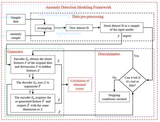
Figure 2. The framework of DAA-GAN.

To assess the effectiveness of the proposed method, this paper employs common evaluation metrics for anomaly detection, as depicted in Figure 3, along with an introduction to anomaly detection. Specifically, this paper considers the following key metrics:

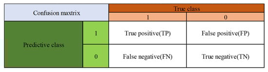
Figure 3. Confusion matrix.

TP is the number of positive samples correctly predicted as positive. FN is the number of positive samples incorrectly predicted as negative. FP is the number of negative samples incorrectly predicted as positive. TN is the number of negative samples correctly predicted as negative. These metrics collectively form the confusion matrix, illustrated in Figure 3. The evaluation indices include Accuracy, Precision, Recall, F1-score (F1), False Alarm Rate (FAR), Missing Alarm Rate (MAR), etc. Their calculations are depicted in Equations (10) and (11).

$$\begin{array}{l}Accuracy={\displaystyle \frac{TP+TN}{TP+FN+FP+TN}},Recall={\displaystyle \frac{TP}{TP+FN}}\\ Precision={\displaystyle \frac{TP}{TP+FP}},F1={\displaystyle \frac{2\cdot Precision\cdot Recall}{Precision+Recall}}\end{array}$$

(10)

$$FAR={\displaystyle \frac{FP}{FP+TN}},MAR={\displaystyle \frac{FN}{FP+FN}}$$

(11)

2.5. Similarity Estimation for Anomaly Assessment

From the anomaly detection stage in the previous step, the anomaly scores of different samples can be obtained, first by calculating the probability distribution of the anomaly scores of different samples, and then by obtaining the probability density distribution graph of the anomaly scores and adopting different similarity analyses to analyses the probability density distributions for similarity analysis, so as to complete the anomaly estimation of the faults, and the specific anomaly estimation framework is shown in the following Figure 4.

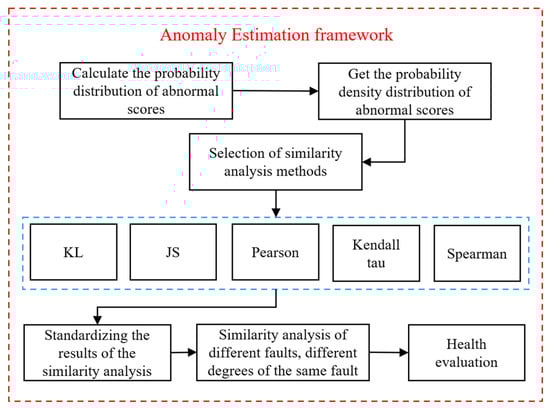
Figure 4. Anomaly estimation framework.

In data science, a similarity metric is a measure of how data samples are related or close to each other. On the other hand, a similarity measure is a way of telling how many of the data objects are different. Also, when similar data samples are grouped into a cluster, these terms are often used for clustering. All other data samples are grouped into different samples. It is also used for classification (e.g., KNN) where data objects are labeled based on the similarity of features. Another example is when discussing outliers that differ from other data samples, such as anomaly detection.

The similarity metric is usually expressed as a numerical value: it is higher when the data samples are more similar. Generally, 0 or 1 is used to indicate the highest degree of similarity; for example, in the KL and JS methods, as the values converge to 0, they become more similar, whereas in Pearson et al.’s methods, as the values converge to 1, they become more similar. Several major methods of similarity analysis are described below.

(1) Kullback–Leibler Divergence

Kullback–Leibler divergence is also known as the KL distance or relative entropy. KL scatter is a way of describing the difference between two probability distributions, P and Q. It is a measure of the degree to which a given distribution deviates from the true distribution, so it can be used to measure the extent to which a given arbitrary distribution deviates from the true distribution. If the two distributions match exactly, then KL (p||q) = 0; otherwise it should take a value between 0 and ∞ (inf). The smaller the KL scatter, the better the match between the true and myopic distributions.

$$KL(p|q)={\displaystyle \sum p}(x)\log {\displaystyle \frac{p(x)}{g(x)}}$$

(12)

(2) Jensen–Shannon Distance

The Jensen–Shannon distance calculates the distance between two probability distributions, p and q. It uses the Kullback–Leibler dispersion (relative entropy) formula to calculate the distance. The value domain of JS dispersion ranges from [0, 1] to 0 for the same and 1 for the opposite.

$$JS(p,q)={\displaystyle \frac{1}{2}}KL(p||{\displaystyle \frac{p+q}{2}})+{\displaystyle \frac{1}{2}}KL(q||{\displaystyle \frac{p+q}{2}})$$

(13)

(3) Pearson Correlation Coefficient

Pearson’s linear correlation coefficient is the most used linear correlation coefficient. The most applicable form of data is linear data, which is continuous and conforms to the normal distribution, and the difference between data cannot be too large. There are m objects and n columns of indicators, which can form the data matrix $X = (x_{ij}{)}_{m \times n}$; now we study the correlation between column a, $x_a$, and column b, $x_b$. Let the correlation coefficients of columns a and b be $rho(a,b)$.

$$rho(a,b)={\displaystyle \frac{{\displaystyle \sum _{i=1}^m(x_{i,a}-{\overline{x}}_a)(x_{i,b}-\overline{x_b})}}{{\displaystyle \sum _{i=1}^m{(x_{i,a}-\overline{x_a})}^2}{\displaystyle \sum _{j=1}^m{(x_{i,b}-{\overline{x}}_b)}^2}}}$$

(14)

(4) Kendall Correlation Coefficient

The Kendall tau correlation coefficient is also a rank correlation coefficient, although it is calculated for categorical variables and applies to both variables. Based on the analysis of the data matrix mentioned in the Pearson correlation coefficient, the Kendall tau coefficient is based on the counts of (i, j) homoscedastic pairs (where i < j), homoscedastic means that $x_{a,i}-x_{a,j}$ and $x_{b,i}-x_{b,j}$ have the same sign. The Kendall tau equations include an adjustment term for the knot value in the normalized constant, often called tau-b. For column a, $x_a$, and column b, $x_b$, of the matrix, the Kendall tau coefficients are defined as

$$\tau ={\displaystyle \frac{2K}{m(m-1)}}$$

(15)

$$K={\displaystyle \sum _{l=1}^{m-1}{\displaystyle \sum _{j=i+1}^m\xi }}$$

(16)

$$\xi =\{\begin{array}{ccc}1& if& (x_{a,i}-x_{a,j})(x_{b,i}-x_{b,j})>0\\ 0& if& (x_{a,i}-x_{a,j})(x_{b,i}-x_{b,j})=0\\ -1& if& (x_{a,i}-x_{a,j})(x_{b,i}-x_{b,j})<0\end{array}$$

(17)

The value of the correlation coefficient ranges from −1 to +1. A value of −1 means that one column order is the inverse of the other, and a value of +1 means that the two column orders are the same. A value of 0 indicates that there is no relationship between the columns.

(5) Spearman’s Rank Correlation Coefficient

Spearman’s rank correlation coefficient is applied to two columns of variables with a hierarchical variable nature of data with a linear relationship, which can well deal with the same values and outliers in the sequence. Based on the data matrix mentioned in the Pearson correlation coefficient for analysis, the Spearman equivalent is applied to the Pearson linear correlation coefficient for the order of columns $x_a$ and $x_b$. For the correlation between column a, $x_a$, and column b, $x_b$, in the matrix, let the correlation coefficient for columns a, and b be $rho(a,b)$.

$$rho(a,b)=1-{\displaystyle \frac{6{\displaystyle \sum d^2}}{m(m^2-1)}}$$

(18)

where d is the difference between the ranks of the two columns and m is the length of each column.

The raw outputs of different similarity measures have different ranges and, more importantly, different directions. For KL/JS divergences, smaller values indicate higher similarity, whereas for correlation coefficients (Pearson/Kendall/Spearman), larger values indicate higher similarity. To ensure the physical meaning of the fused score is consistent, a two-step processing is adopted before fusion: (i) directional alignment, which converts all measures into similarity scores where a larger value always means ‘more similar’; and (ii) normalization, which scales the aligned similarity scores to a comparable range (0–1) prior to fusion.

(6) Directional alignment

Directional alignment is performed as follows. For divergence-type measures (KL/JS), let $d_i$ be the divergence between a test distribution and the $i$-th reference distribution. We first apply Min-Max scaling across the candidate reference set and then invert it to obtain a similarity score:

$$d_i^{\mathrm{norm}}={\displaystyle \frac{d_i-\min (d)}{\max (d)-\min (d)+\epsilon }},\hspace{1em}{s}_i^{\mathrm{div}}=1-d_i^{\mathrm{norm}}$$

(19)

(7) $\mathbf{d}= \left\{d_i\right\}$ is the set of divergences over all candidate references, and $\epsilon$ is a small constant to avoid division by zero. Correlation-type measures (Pearson/Kendall/Spearman). For correlation coefficients $r_i \in [-1, 1]$, we map them into [0, 1] by

$$s_i^{\mathrm{corr}}={\displaystyle \frac{r_i+1}{2}}$$

(20)

After this alignment, all similarity scores are further normalized using Equation (21) when necessary.

(8) Normalization

Where $x$ is an aligned similarity score (after directional alignment), $x_{\mathrm{norm}}$ is the normalized score in $\left[0,1\right]$, $\mathrm{m}\mathrm{a}\mathrm{x}\left(\mathbf{x}\right)$ and $\mathrm{m}\mathrm{i}\mathrm{n}\left(\mathbf{x}\right)$ are the maximum and minimum values in the candidate reference set, and $\epsilon$ is a small constant to avoid division by zero:

$$x_{\mathrm{norm}}={\displaystyle \frac{x-\min (x)}{\max (x)-\min (x)+\epsilon }}$$

(21)

(9) Fusion of multi-index similarity scores

After directional alignment and normalization, the similarity scores from the five methods are fused to obtain an overall similarity for fault assessment. In this study, a weighted average is adopted (equal weights by default). After the standardization of the analysis results, the five similarity indicators need to be fused, and the fused indicators $S_j$ are compared to come to the fault assessment. The specific fusion formula is:

$$S_{\mathrm{fuse}}(j)={{\displaystyle \sum }}_{i=1}^m{w}_i{s}_i(j),\hspace{1em}{{\displaystyle \sum }}_{i=1}^m{w}_i=1$$

(22)

where $S_{\mathrm{fuse}}\left(j\right)$ is the fused similarity score, $m$ is the number of similarity measures, $w_i$ is the weight of the $i$-th measure, and $s_i\left(j\right)$ is the aligned-and-normalized similarity score of the $i$-th measure for the $j$-th reference. Where $S_j$ is the fused similarity metric, $m$ is the number of similarity analysis methods, $B_j$ is the known (reference) data, $Z$ is the test data, and $S_i$ is the analysis result of a single similarity analysis method. The pseudocode for Algorithm 1 is shown below.

Algorithm 1. Multi-index similarity fusion for Stage III

Input: anomaly-score sequence of a test sample $A_{\mathrm{test}}$ and reference anomaly-score sequences $\left\{A_{\mathrm{ref}}\left(k\right)\right\}$ for each fault class/severity k.

Output: $k^{*}={\mathrm{argmax}}_k{S}_{\mathrm{fuse}}\left(k\right)$ as the identified fault type/severity.

Step 1: Estimate the probability density distributions $P_{\mathrm{test}}$ and $\left\{P_{\mathrm{ref}}\left(k\right)\right\}$ (e.g., by kernel density estimation or histogram normalization).

Step 2: Compute raw metrics for each $k: {KL}_k, {JS}_k, {r_k}^P, {r_k}^K, {r_k}^S.$

Step 3 (Directional alignment): Convert divergences to similarities using       $s_{KL}\left(k\right)=1-\mathrm{MinMax}\left(K{L}_k\right),s_{JS}\left(k\right)=1-\mathrm{MinMax}\left(J{S}_k\right),$ and convert correlations using        $s_P\left(k\right)={\displaystyle \frac{r_k^P+1}{2}},s_K\left(k\right)={\displaystyle \frac{r_k^K+1}{2}},s_S\left(k\right)={\displaystyle \frac{r_k^S+1}{2}}.$

Step 4 (Optional normalization): Apply Equation (21) to normalize each aligned similarity vector across k.

Step 5 (Fusion): Fuse the aligned-and-normalized similarities by        $S_{\mathrm{fuse}}\left(k\right)={\displaystyle {\displaystyle \sum }_{i=1}^m}{w}_i\hspace{0.17em}{s}_i\left(k\right).$

Step 6 (Decision): Output $k^{*}={\mathrm{argmax}}_k{S}_{\mathrm{fuse}}\left(k\right)$. as the identified fault type/severity.

Numerical example (illustrative). Suppose three references yield $KL=[0.20,\hspace{0.17em}0.50,\hspace{0.17em}0.80]$. Then $\mathrm{MinMax} \left(KL\right)=[0,\hspace{0.17em}0.5,\hspace{0.17em}1]$ and the aligned similarities are $s_{KL}=[1.0,\hspace{0.17em}0.5,\hspace{0.17em}0.0]$. If Pearson $r=[0.95,\hspace{0.17em}0.60,\hspace{0.17em}0.10]$, then $s_P=(r+1)/2=[0.975,\hspace{0.17em}0.80,\hspace{0.17em}0.55]$. After normalization and equal-weight fusion, the reference with the largest $S_{\mathrm{fuse}}$ is selected as the closest fault severity.

3. Validation

3.1. A Simulation Case of the Split-Torque Transmission System

The split-torque transmission system represents a typical multi-path gear transmission configuration that is widely employed in helicopter gearboxes, naval propulsion systems, and other high-power-density rotating machinery drive chains. Compared to conventional single-path transmissions, split-torque transmissions distribute and combine input power through multiple parallel paths, offering advantages such as high power density, high transmission efficiency, and excellent redundancy. However, the presence of multiple meshing pairs and multi-path couplings also complicates fault mechanisms and vibration responses, posing challenges for fault detection and severity assessment. To systematically evaluate the performance of the proposed phased anomaly detection and assessment framework under controlled conditions, this paper first constructs a simulation case using a torque-splitting gear transmission system, whose structural schematic is shown in Figure 5. Subsequently, Section 3.1.1 presents the fault simulation model for this system.

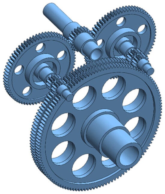
Figure 5. A split-torque transmission system.

3.1.1. Split-Torque Transmission System and Its Simulation Model

A split-torque transmission system is illustrated in Figure 5. The system adopts a two-stage transmission architecture. In the input stage, an input pinion simultaneously meshes with two identical large spur gears, thereby splitting the input power into two parallel paths. In the output stage, two identical pinions on the duplex shafts simultaneously mesh with the output large spur gear, recombining the transmitted torque at the output. In this configuration, the two duplex gear shafts constitute the two power branches of the split-torque system.

When the potential energy method is used to compute gear meshing stiffness, the gear tooth is commonly idealized as a two-dimensional cantilever beam with a variable cross-section, as shown in Figure 6.

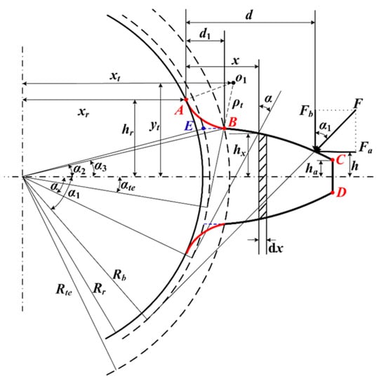
Figure 6. Variable cross-section cantilever-beam model of an involute spur-gear tooth (used to derive tooth stiffness and the time-varying meshing stiffness in the dynamic simulation).

Figure 6 presents the beam-based formulation for evaluating tooth bending stiffness, which is subsequently incorporated into the time-varying meshing stiffness of the gear-pair model. Variations in meshing stiffness provide the primary mechanism by which tooth-root crack growth or tooth breakage alters the simulated vibration response. The resulting time-domain response signals serve as inputs to the proposed staged framework: DAA-GAN generates anomaly-score sequences for Stage I–II detection, and the anomaly-score probability density distributions form the basis for similarity-based severity assessment in Stage III.

The gear-tooth profile is composed of three segments: AB represents the root filet (transition arc), BC denotes the involute flank, and CD corresponds to the addendum-circle arc. Point E is the intersection between the involute and the base circle. Point $O_1$ is the center of the transition arc with coordinates (x_t, y_t); Point A marks the start of the transition arc on the root circle with coordinates (x_r, h_r); and point B is the end of the transition arc. The parameter $\mathrm{d}$ denotes the equivalent cantilever length, defined as the distance from the meshing point to the tooth root. The load $\mathrm{F}$ is the force acting normal to the meshing surface, and ${\alpha }_1$ is the angle between $\mathrm{F}$ and the vertical direction (i.e., the tooth-thickness direction). The quantities $h$, $h_x$, and $h_a$ denote the distances from the tooth profile to the neutral axis at the meshing point, at position $x$, and at the addendum circle, respectively. Moreover, $R_r$, $R_b$, and $R_{te}$ denote the radii of the root circle, base circle, and the transition-arc endpoint circle at point B, respectively.

As tooth-root cracks propagate to a critical extent, local tooth fracture may occur, which is referred to as a broken-tooth fault. When the fracture develops along the face-width direction, the stiffness components of an intact tooth—namely the bending stiffness, shear stiffness, axial compressive stiffness, Hertzian contact stiffness, and gear-body stiffness—indicate that each sub-stiffness term is linearly proportional to the tooth face width $L$. Accordingly, the meshing stiffness of a fractured tooth can be obtained by replacing the intact face width $L$ with the remaining effective face width $L_{\mathrm{b}\mathrm{r}\mathrm{o}\mathrm{k}\mathrm{e}\mathrm{n}}$ in the corresponding stiffness expressions. The meshing stiffness $k_{\mathrm{b}\mathrm{r}\mathrm{o}\mathrm{k}\mathrm{e}\mathrm{n}}$ of the fractured tooth is therefore calculated as follows:

$${\displaystyle \frac{1}{k_{broken}}}={\displaystyle \frac{1}{k_h}}+{\displaystyle \frac{1}{k_{b1,broken}}}+{\displaystyle \frac{1}{k_{a1}}}+{\displaystyle \frac{1}{k_{s1,broken}}}+{\displaystyle \frac{1}{k_{f1}}}+{\displaystyle \frac{1}{k_{b2}}}+{\displaystyle \frac{1}{k_{a2}}}+{\displaystyle \frac{1}{k_{s2}}}+{\displaystyle \frac{1}{k_{f2}}}$$

(23)

where $k_h$ is the elastic contact deformation of the contact surface during gear meshing, the corresponding Hertzian contact stiffness; $k_{b1,\mathit{broken}}$ is the bending stiffness of the gear tooth in the broken tooth state; $k_{a1}$ is the axial compression stiffness of the gear tooth; $k_{s1,\mathit{broken}}$ is the shear stiffness of the gear tooth in the broken tooth state; $k_{f1}$ is the stiffness of the gear wheel body; $k_{b2}$ is the bending stiffness of the gear tooth; $k_{a2}$ is the axial compression stiffness of the gear tooth; $k_{s2}$ is the shear stiffness of the gear tooth; $k_{f2}$ is the stiffness of the gear wheel body.

Specific parameters for these gears are provided in Table 1. Gear 1 is the input, with an input speed of 7050 revolutions per minute. The drive train is rated at 500 kW. k_bx and k_by denote the stiffness coefficients of the bearing in the X-axis and Y-axis directions, respectively. The parameters of the Split-torque transmission are shown in Table 1.

Table 1. Split-torque transmission system parameters.

Parameters	Gear1	Gear2/Gear3	Gear2/Gear3	Gear6
Number of teeth	21	70	13	126
Pressure angle (°)	22.5	22.5	25	25
Module (mm)	4.5	4.5	4.5	4.5
Face width (mm)	30	30	80	80
Inertia (kg∙mm2)	1832.1	2.26 × 105	717.5	6.33 × 106
Weight (kg)	1.64	18.24	1.68	>157.56
Bearing stiffness (N/m)	kbx = kby = 1 × 108

Mark the split-torque transmission system orientation as shown in Figure 7 to divide the drive train into front and rear (FWD, AFT) branches. Mark the input small spur gear, the input large spur gear (FWD, AFT), the output small spur gear (FWD, AFT), and the output large spur gear in the system as gears 1 to 6 in that order.

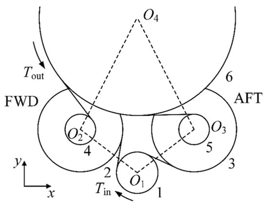
Figure 7. Schematic diagram of a split-torque transmission system.

A generalized coordinate system of the transmission system is established with the rotary center O₂ of gear 2 pointing to the rotary center O₃ of gear 3 as the x-axis positive direction, and the rotary center O₁ of gear 1 pointing to the rotary center O₄ of gear 6 as the y-axis positive direction. Each gear contains x, y, and θ degrees of freedom. For any two of these gear pairs (gear i and gear j) that mesh with each other, an expression for their gear mesh force can be written as follows:

$$F_g=k_g{\delta }_{ij}+c_g{\dot{\delta }}_{ij}$$

(24)

where $k_g$ is the time-varying meshing stiffness of the gears; ${\dot{\delta }}_{ij}$ is the counterclockwise angle from the y-axis positive to the positive direction of the meshing line (gear i pointing to gear j). ${\dot{\delta }}_{ij}$ is the dynamic transfer error, which is expressed as:

$${\delta }_{ij}=x_i\sin {\phi }_{ij}-y_i\cos {\phi }_{ij}+r_i{\theta }_i-x_j\sin {\phi }_{ij}+y_j\cos {\phi }_{ij}-r_j{\theta }_j$$

(25)

According to Newton’s second theorem, the dynamic equation of the meshing pair consisting of gear i and gear j can be written as:

$$m_i{\ddot{x}}_i+c_i{\dot{x}}_i+k_i{x}_i=-F_g\sin {\phi }_{ij}$$

(26)

$$m_i{\ddot{y}}_i+c_i{\dot{y}}_i+k_i{y}_i=F_g\cos {\phi }_{ij}$$

(27)

$$J_i{\ddot{\theta }}_i=-F_g{r}_i$$

(28)

$$m_j{\ddot{x}}_j+c_j{\dot{x}}_j+k_j{x}_j=F_g\sin {\phi }_{ij}$$

(29)

$$m_j{\ddot{y}}_j+c_j{\dot{y}}_j+k_j{y}_j=-F_g\cos {\phi }_{ij}$$

(30)

$$J_j{\ddot{\theta }}_j=F_g{r}_j$$

(31)

After obtaining the kinetic equations of each gear meshing pair, the kinetic equations of each meshing pair are assembled and converted into matrix form to obtain the kinetic equations of the whole torsion split transmission system as follows:

$$M\ddot{x}+C\dot{x}+Kx=F$$

(32)

where the total stiffness matrix, K = K_m + K_c + K_xy, is the sum of the gear meshing stiffness matrix, the coupling stiffness matrix between gears, and the support stiffness matrix of the bearings; C is the damping matrix; M is the mass matrix; F is the external load matrix; and x is the vector of degrees of freedom of the system:

$$x={\left[x_1,y_1,{\theta }_1,x_2,y_2,{\theta }_2,\dots ,x_6,y_6,{\theta }_6\right]}^{\mathrm{T}}$$

(33)

3.1.2. Anomaly Detection and Threshold Optimization

Normal and abnormal data were collected in experiments conducted at different rotational speeds for gears in a split torque transmission system. To differentiate between the two, different data samples were processed through the model, resulting in different evaluation scores. Depending on whether the score was high or low, it was determined whether the data was normal or abnormal. The result of the threshold selection determined this distinction, as shown in Figure 8. Figure 8 shows the Split-torque transmission system’s relationship between the error (FAR, MAR) and the threshold.

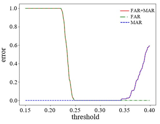
Figure 8. Relationship between torque transmission system error and threshold.

3.1.3. Anomaly Evaluation

In the split-torque simulation case, we consider fracture-related fault scenarios and organize them into severity-level classes for evaluation. Particularly, each fault mode is parameterized into 10 severity levels (Level 1 to Level 10), and 120 samples are generated for each level. The physical definitions of the 10 severity levels for fracture-related faults (and their corresponding stiffness-degradation interpretation) are provided in Appendix B Table A1. Specifically, the broken-tooth severity is implemented by replacing the tooth face width $L$ with $L_{\mathrm{broken}}$ in the stiffness expressions (Table A1(a)), while the tooth-root crack severity is parameterized by the crack depth $a$ in the cantilever-beam model (Table A1(b)).

Each sample used in the simulation study is a fixed-length time-domain vibration-response segment generated by numerically integrating the split-torque dynamic model under the specified operating conditions. The simulated vibration response is recorded at a constant sampling rate of $f_s = \mathrm{20,000}$ Hz and then segmented into non-overlapping windows of $N=2048$ points (i.e., a window duration of $N/f_s = 0.1024$ s), which are used as the input samples for subsequent modeling and evaluation. For each severity level, 120 samples are obtained in a reproducible manner by conducting repeated simulations with different initial phases and independent noise realizations to reflect variability, and extracting multiple non-overlapping windows from the steady-state portion of the simulated response so that exactly 120 segments are collected per level. Unless otherwise stated, the model is trained using normal-condition samples only, whereas validation and testing are performed on disjoint (non-overlapping) sample sets containing both normal and faulty conditions to compute FAR/MAR and the corresponding detection accuracy.

In the following, the broken tooth fault is mainly analyzed. In Figure 9 and Figure 10, the samples of different faults are colored differently, the color is from purple to red, the degree of the fault is deepening, the abnormality scores of the model output are increasing, and the corresponding density distributions are also different. Comparing Figure 9 and Figure 10, the anomaly scores of cracked faults in both Gear 1 and Gear 2 tend to increase with the increase in fault grade. However, the probability density curves for the 10 fault classes in Gear 1 are more discriminating than those in Gear 2. This difference may be because the vibration shocks in Gear 2 are weaker and the vibration shocks transmitted to Gear 1 have very little loss in the transmission path and are therefore less distinguishable.

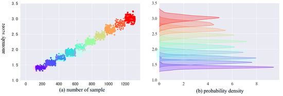
Figure 9. Gear 1 broken fault anomaly score and probability density.

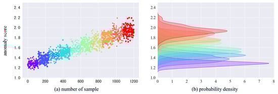
Figure 10. Gear 2 broken fault anomaly score and probability density.

To support the detection-performance statement quantitatively, fracture-fault detection is formulated as a binary decision based on the DAA-GAN anomaly score $s$. Specifically, normal-condition samples are treated as the negative class, whereas fracture-related fault samples (across the 10 severity levels) are treated as the positive class. A test sample is classified as faulty if $s > \tau$, where the threshold $\tau$ is selected in Stage II by analyzing the FAR–MAR trade-off on disjoint validation sets that contain both normal and fault samples (Figure 8). For clarity of presentation, we further report a normalized anomaly score $\widetilde{s }= s/\tau$, such that the decision threshold becomes $\tilde{\tau } = 1$ (i.e.,$>1$ indicates a fault). Note that Figure 9 and Figure 10 visualize the anomaly-score distributions of the ten fault severity levels; the detection conclusion is not inferred from the plots alone, but is validated by the confusion-matrix statistics on the held-out test set. Accordingly, detection accuracy is computed as:

$$Accuracy={\displaystyle \frac{TP+TN}{TP+TN+FP+FN}}$$

(34)

where $TP$, $TN$, $FP$, and $FN$ denote true positives, true negatives, false positives, and false negatives, respectively. In addition, the false alarm rate and miss alarm rate are defined as $\mathrm{FAR}= FP/(FP+TN)$ and $\mathrm{MAR}= FN/(FN+TP)$.

Under the adopted protocol, the final detection performance is evaluated on a held-out test set that contains both normal-condition samples (negative class) and fracture-related fault samples (positive class). The training, validation, and test sets are disjoint and non-overlapping, ensuring that no signal segments are shared across splits and thus avoiding information leakage. After obtaining the anomaly score for each test sample, we apply the decision rule using $\tilde{s} = s/\tau$ with $\tilde{\tau } = 1$, and assign the predicted label $\widehat{y}$ as:

$$\widehat{y}=\{\begin{array}{cc}1,& \overline{s}>1\hspace{1em}\left(\mathrm{fault}\right),\\ 0,& \overline{s}\le 1\hspace{1em}\left(\mathrm{normal}\right)\end{array}$$

(35)

The confusion-matrix entries are then computed by sample-wise counting on the test set: $TN$ is the number of normal samples satisfying $\tilde{s} \le 1$, $FP$ is the number of normal samples satisfying $\tilde{s} > 1$, $TP$ is the number of fracture-fault samples satisfying $\widetilde{s }> 1$, and $FN$ is the number of fracture-fault samples satisfying $\tilde{s} \le 1$. Therefore, FAR and MAR directly quantify the misclassification counts on the negative and positive classes, respectively.

In the simulated fracture-fault experiments, the held-out test set contains 120 normal-condition samples and 2400 fracture-fault samples (Gear 1 and Gear 2, Levels 1–10; 120 samples per level, i.e., $2\times 10\times 120$). Under the selected threshold, all 120 normal test samples satisfy $\tilde{s}\le 1$, yielding $TN =120$ and $FP =0$; meanwhile, all 2400 fracture-fault test samples satisfy $\widetilde{s }>1$, yielding $TP =2400$ and $FN =0$. Therefore, $\mathrm{FAR}=0$, $\mathrm{MAR}=0$, and $\mathrm{A}\mathrm{c}\mathrm{c}\mathrm{u}\mathrm{r}\mathrm{a}\mathrm{c}\mathrm{y}=1.0$, which supports the reported 100% detection accuracy under the adopted evaluation protocol.

The following five similarity analysis methods were used to correlate the different failure cases of Gear 1 and Gear 2. Plots (a), (b), (c), (d), and (e) in Figure 11 and Figure 12 represent the results of five similarity analysis methods, namely KL distance, JS distance, Pearson’s correlation coefficient, Kendall’s tau correlation coefficient and Spearman’s correlation coefficient, for the different breakage failure classes (G1–G10) of Gear 1 and Gear 2, respectively. From the results, there is a good differentiation between the different degrees of failure. The KL distance analysis method gives better results for the type of fracture failure. Overall, Gear 1 shows higher discrimination at each failure level, while Gear 2 shows lower discrimination at neighboring failure levels.

Figure 11. Gear 1 broken fault correlation analysis results.

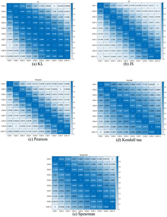
Figure 12. Gear 2 broken fault correlation analysis results.

Taking gear 1 as an example, the test data G1test is utilized for evaluation using the DAA-GAN model. Firstly, the anomaly score is computed for the test data, followed by obtaining the probability density plot of the anomaly scores, as depicted in Figure 13.

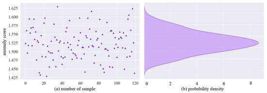
Figure 13. Test data anomaly score and probability density.

Subsequently, similarity analysis is conducted between the test data and known data, and the results of this analysis are normalized. Figure 14 illustrates the standardized results of the similarity analysis. During the assessment phase, the standardized similarity metrics between the test data and known data are integrated. The evaluation reveals that the test data most closely resembles the fault condition represented by G1B-2, as detailed in Table 2. From Table 2, it is evident that the test data exhibits the highest similarity with G1B-2, suggesting the fault condition of the test data corresponds to G1B-2.

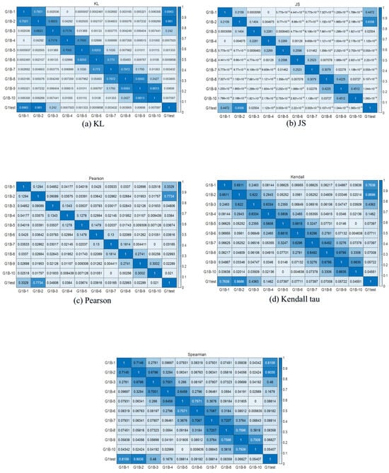
Figure 14. Test data correlation analysis results.

Table 2. Overall similarity results between test samples and reference samples for each fault level.

Subjects	G1B-1	G1B-2	G1B-3	G1B-4	G1B-5
Similarity	0.623096	0.873446	0.198775	0.051758	0.031555
Subjects	G1B-6	G1B-7	G1B-8	G1B-9	G1B-10
Similarity	0.032992	0.030805	0.029354	0.024305	0.020541

3.2. Validation with Popular Open Datasets

3.2.1. CWRU Dataset

Rolling bearing vibration data were acquired from the Case Western Reserve University (CWRU) Bearing Data Center [32], which is widely used as a benchmark dataset for bearing fault diagnosis and anomaly detection [33]. In this work, we use the drive-end accelerometer signals sampled at 48 kHz under three operating speeds (1730, 1750, and 1772 rpm). The dataset includes normal condition and three fault types: inner race (IR), rolling element (Ball), and outer race (OR) faults. Fault diameters are 0.007, 0.014, and 0.021 inch, and OR faults are located at 3, 6, and 12 o’clock positions. Figure 15 shows the CWRU test bed, and Table 3 summarizes the key settings and the subset configuration adopted in this study.

Figure 15. Testing bed of CWRU.

Table 3. CRWU dataset description.

Parameter	Value
Sampling Frequency (kHz)	12, 48
Motor speed (RPM)	1730, 1750, 1772, 1797
Fault type	IR, OR, B
Fault size(inch)	0.007, 0.014, 0.021
Fault implantation direction	3, 6, 12

Within the proposed framework, the CWRU drive-end vibration signals are segmented into fixed-length time-domain windows and fed into DAA-GAN for unsupervised anomaly detection; as labeled fault data accumulate, the anomaly-score probability density distributions are further utilized for similarity-based severity assessment in Stage III.

3.2.2. Anomaly Detection and Threshold Optimization

In the experiments conducted on the CWRU drive end rolling bearing under various speeds, both normal and abnormal samples were collected.

To distinguish between the two, different data samples were processed through the model, resulting in distinct evaluation scores. Based on the scores being either high or low, the determination of whether the data is normal or abnormal is made. The results of threshold selection, which determine this distinction, are depicted in Figure 16.

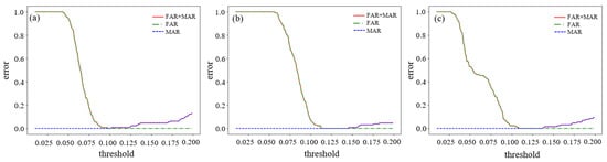
Figure 16. Error threshold relationships on the CWRU dataset: (a) condition 1; (b) condition 2; (c) condition 3.

3.2.3. Anomaly Evaluation

Figure 16 shows the change in error for RPM1730, RPM1750, and RPM1772 operating conditions, represented by plots (a), (b), and (c), respectively, as the threshold is varied. The horizontal axis represents the threshold value, while the vertical axis represents the error. The green dotted and blue dashed lines show the curves of FAR and MAR relative to the threshold, respectively, and the red solid line shows the sum of the errors of the two ratios.

In the initial stage, when the equipment is operating normally and only normal data samples are available, continuous adjustment of the threshold leads to a gradual decrease in the false alarm rate, approaching zero.

In the second stage, as equipment failures occur to a limited extent, the threshold value continues to increase, causing the leakage alarm rate to rise. The threshold value within the range of low total error is used to assess the abnormal scores of the test set’s outputs, with values exceeding this threshold classified as abnormal.

In the third stage, as the number of faults increases and a substantial amount of fault data is collected, fault categories are determined based on the probability distributions of different anomaly scores. The results of the anomaly scores and density plots are illustrated in Figure 17, Figure 18 and Figure 19.

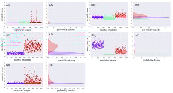
Figure 17. RPM 1730 anomaly score and probability density: (a1) anomaly scores for case A; (a2) probability density of anomaly scores for case A; (b1) anomaly scores for case B; (b2) probability density of anomaly scores for case B; (c1) anomaly scores for case C; (c2) probability density of anomaly scores for case C; (d1) anomaly scores for case D; (d2) probability density of anomaly scores for case D; (e1) anomaly scores for case E; (e2) probability density of anomaly scores for case E.

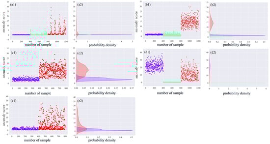
Figure 18. RPM 1750 anomaly score and probability density: (a1) anomaly scores for case A; (a2) probability density of anomaly scores for case A; (b1) anomaly scores for case B; (b2) probability density of anomaly scores for case B; (c1) anomaly scores for case C; (c2) probability density of anomaly scores for case C; (d1) anomaly scores for case D; (d2) probability density of anomaly scores for case D; (e1) anomaly scores for case E; (e2) probability density of anomaly scores for case E.

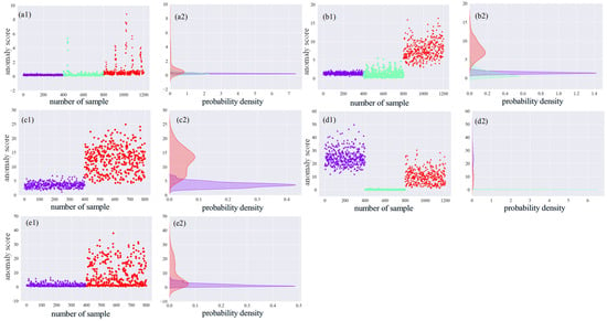
Figure 19. RPM 1772 anomaly score and probability density: (a1) anomaly scores for case A; (a2) probability density of anomaly scores for case A; (b1) anomaly scores for case B; (b2) probability density of anomaly scores for case B; (c1) anomaly scores for case C; (c2) probability density of anomaly scores for case C; (d1) anomaly scores for case D; (d2) probability density of anomaly scores for case D; (e1) anomaly scores for case E; (e2) probability density of anomaly scores for case E.

In each of the graphs in Figure 17, Figure 18 and Figure 19, the labels (a1), (a2), (b1), and (b2) represent the anomaly scores and probability densities of rolling body faults and inner ring faults for various operating conditions. Meanwhile, the labels (c1), (c2), (d1), (d2), and (e1), (e2) represent the anomaly scores and probability densities of outer ring faults, each corresponding to different fault placements. Additionally, each fault type has a distinct fault diameter. To distinguish them, this paper uses purple to indicate 0.007-inch faults, light green to indicate 0.014-inch faults, and red again to indicate 0.021-inch faults.

In the (a1), (b1), (c1), (d1), and (e1) plots of Figure 17, Figure 18 and Figure 19, the horizontal coordinates represent the total number of tests set samples, while the vertical coordinates represent the sample anomaly scores. The red dashed line represents the threshold value. In the (a2), (b2), (c2), (d2), and (e2) plots of Figure 17, Figure 18 and Figure 19, density plots for different faults are presented. The horizontal axis represents the probability, and the vertical axis represents the anomaly score. The probability density plots in Figure 17, Figure 18 and Figure 19 demonstrate that different fault sizes within the same fault type are well distinguished. However, some distinct faults are modeled with probability densities that appear more similar, leading to challenges in differentiation.

The graphs show variations in probability density distributions among different fault categories. For instance, in the (a1) plots of Figure 17, Figure 18 and Figure 19, the anomaly scores for 0.007 inches, 0.014 inches, and 0.021 inches of rolling body faults exhibit an increasing trend. On the other hand, inner ring faults are differentiated based on fault levels and exhibit distinct density distributions. For outer ring faults at 3 o’clock and 12 o’clock directions within the loaded area, deeper degrees of failure result in higher overall anomaly scores. However, for the 6 o’clock direction orthogonal to the loaded area, anomalies at 0.014 inches yield smaller output fractions. Notably, the distributions for 0.007 inches and 0.021 inches of outer ring faults differ significantly. The accuracy of anomaly detection is summarized in Table 4.

Table 4. Detection accuracy on the CWRU dataset (Mean ± Std across three speeds).

	Accuracy
Fault Type	N	Ball			IR			OR
Fault Direction	\	07	14	21	07	14	21	3		6			12
Fault Size								07	21	07	14	21	07	21
RPM1730	1.000	1.000	1.000	1.000	1.000	0.993	1.000	1.000	1.000	1.000	0.998	1.000	1.000	1.000
RPM1750	1.000	1.000	0.983	1.000	1.000	1.000	1.000	1.000	1.000	1.000	1.000	1.000	1.000	1.000
RPM1772	1.000	1.000	0.955	1.000	1.000	1.000	1.000	1.000	1.000	1.000	0.998	1.000	1.000	1.000
Mean	1.000	1.000	0.979	1.000	1.000	0.998	1.000	1.000	1.000	1.000	0.999	1.000	1.000	1.000
Std	0.000	0.000	0.023	0.000	0.000	0.004	0.000	0.000	0.000	0.000	0.001	0.000	0.000	0.000

As indicated in Table 4, most anomalies can be successfully detected across operating conditions, with an overall average detection accuracy of 99.83% on the CWRU dataset. To improve the rigor of result reporting, Table 4 also reports the mean and standard deviation (Std) across the three operating speeds (1730/1750/1772 rpm). The main performance degradation is observed for the Ball fault with 0.014-inch diameter (minimum accuracy 0.955 at 1772 rpm), while the remaining fault categories achieve near-perfect accuracy with low variance.

In this paper, five similarity analysis methods are used to analyze the similarity between different fault-type distribution patterns observed under various operating conditions. This helps determine the degree of resemblance between the new faults and existing fault categories. It also calculates the accuracy of fault classification, facilitating fault identification. Firstly, five correlation analysis methods are used to analyze the three types of faults at 1730 RPM, and the results are shown in Figure 20, Figure 21 and Figure 22. In plots (a), (b), (c), (d), and (e) of Figure 20, Figure 21 and Figure 22, which represent the results of the five methods of similarity analysis, namely KL distance, JS distance, Pearson correlation coefficient, Kendall tau correlation coefficient, and Spearman correlation coefficient, respectively. For rolling body defects, as shown in Figure 20, the JS method gives the best results, while for inner ring defects, as shown in Figure 21, the Spearman method gives better results, and for outer ring 6 o’clock defects, as shown in Figure 22, the Pearson method gives better results.

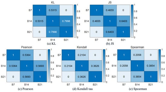
Figure 20. RPM1730 Ball correlation analysis results.

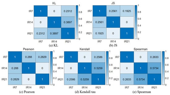
Figure 21. RPM1730 IR correlation analysis results.

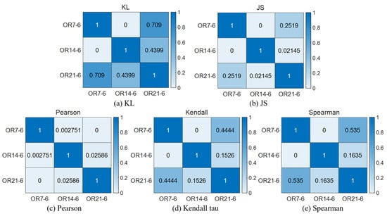
Figure 22. RPM1730 OR6 correlation analysis results.

In the context of the RPM1730 operating condition, with the fault type being a 6 o’clock position defect on the rolling element, test data “test” was analyzed using the DAA-GAN model. Initially, the anomaly scores were calculated, leading to the generation of a probability density graph of the anomaly scores, as represented in Figure 23, which illustrates the anomaly scores and the probability density graph of the test data. Subsequently, the test data was subjected to a similarity analysis with known data, and the results of this analysis were normalized. Figure 24 showcases the results of the similarity analysis after normalization. In the evaluation phase, the normalized similarity indices between the test data and the known data were fused to assess the fault condition most like that of the test data. The assessment results, as documented in Table 5, indicate a higher similarity of the test data with OR7-6. Based on this analysis, it can be inferred that the fault condition of the test data corresponds to OR7-6.

Figure 23. Test data anomaly score and probability density.

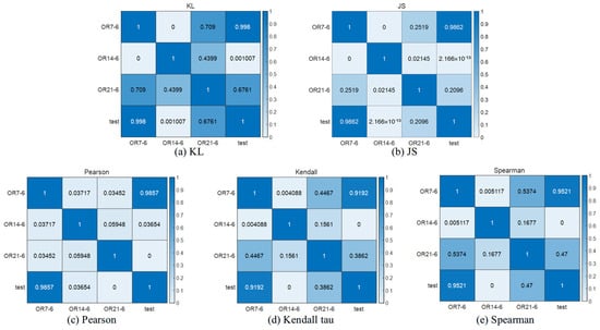
Figure 24. Test data correlation analysis results.

Table 5. Comprehensive similarity evaluation results.

Subjects	OR7-6	OR14-6	OR21-6
Similarity	0.96824	0.007308	0.34838

3.2.4. Comparison with Related Methods on the CWRU Dataset

Since the CWRU dataset has been widely used in bearing diagnostics, we further compare the proposed DAA-GAN framework with representative methods reported in the recent literature. Table 6 summarizes the published results. Note that CWRU performance is sensitive to data preprocessing, class definition and data splitting strategy; therefore, the comparison is indicative rather than strictly identical.

Table 6. Comparison with representative methods on the CWRU dataset (indicative).

Method	Learning Paradigm	Key Idea	Metric (Reported)	Reported Performance on CWRU
FaultFace (DCGAN-aided) [10]	Supervised (GAN-aided)	Data augmentation + CNN classifier	Accuracy (best)	100%
WDCAE-LKA [34]	Unsupervised	Autoencoder + large-kernel attention + dynamic threshold	Average diagnostic accuracy	90.29%
ADBR [35]	Self-supervised	BYOL-style representation + reconstruction	Average fault detection accuracy	96.97%
DAA-GAN (this work)	Unsupervised + staged	DAA-GAN + adaptive threshold + similarity fusion	Average detection accuracy (Table 4)	99.83% (1730/1750/1772 rpm)

Recent benchmark studies have also reported that overly optimistic splits may lead to inflated CWRU results; rigorous, leakage-free evaluation remains important for reproducibility [36]. In this paper, we therefore report mean and standard deviation across operating speeds (Table 4) and will further extend benchmarking under stricter split protocols in future work. More importantly, beyond pursuing high accuracy, this study aims to provide a data-accumulation-aware diagnostic framework that remains effective when fault data are unavailable: it enables anomaly detection using normal-condition data only in the initial stage, and progressively improves detection performance as fault data accumulate over the equipment lifecycle.

4. Conclusions

This paper proposes a data-accumulation-aware anomaly detection and severity assessment framework for rotating machinery based on DAA-GAN. By explicitly considering the progressive accumulation of fault data during the equipment lifecycle, the framework integrates unsupervised anomaly detection, adaptive threshold updating, and similarity-based severity evaluation. The main findings and contributions are summarized as follows:

(1) High detection accuracy: The proposed method achieves 100% detection accuracy for the simulated gear tooth breakage levels and an overall average detection accuracy of 99.83% on the CWRU bearing dataset across three operating speeds (1730/1750/1772 rpm). These results demonstrate the effectiveness of DAA-GAN for learning normal patterns and detecting deviations.

(2) Robust performance under imbalanced data: With only a small number of fault samples available (Stage II), the adaptive threshold update strategy selects a decision threshold by minimizing FAR+MAR on a validation set, which improves detection robustness and reduces the sensitivity to operating-condition variation.

(3) Lifecycle-aware staged assessment: When sufficient labeled fault samples are accumulated (Stage III), the proposed multi-index similarity fusion strategy compares anomaly-score distributions between test samples and reference faults, enabling consistent fault type/severity assessment rather than only binary anomaly detection.

Limitations and future work: (i) The current validation method focuses on two case studies and single-sensor vibration signals. More datasets and real industrial deployments are needed to fully verify generalization. (ii) The similarity fusion strategy currently adopts fixed (default equal) weights. Learning adaptive weights or uncertainty-aware fusion is a promising direction. (iii) To further improve reproducibility, future work will conduct more extensive ablation studies and benchmarking under stricter, leakage-free data splits and multiple random seeds and explore online incremental updating for long-term deployment.

References

- Deng, W.; Li, Z.; Li, X.; Chen, H.; Zhao, H. Compound Fault Diagnosis Using Optimized MCKD and Sparse Representation for Rolling Bearings. IEEE Trans. Instrum. Meas. 2022, 71, 1–9. [Google Scholar] [CrossRef]
- Ma, J.; Shang, J.; Zhao, X.; Zhong, P. Bayes-DCGRU with bayesian optimization for rolling bearing fault diagnosis. Appl. Intell. 2022, 52, 11172–11183. [Google Scholar] [CrossRef]
- Shao, H.; Xia, M.; Wan, J.; de Silva, C.W. Modified Stacked Autoencoder Using Adaptive Morlet Wavelet for Intelligent Fault Diagnosis of Rotating Machinery. IEEE/ASME Trans. Mechatron. 2022, 27, 24–33. [Google Scholar] [CrossRef]
- Zhou, P.; Hu, X.; Li, P.; Wu, X. Online feature selection for high-dimensional class-imbalanced data. Knowl.-Based Syst. 2017, 136, 187–199. [Google Scholar] [CrossRef]
- Viola, J.; Chen, Y.; Wang, J. FaultFace: Deep convolutional generative adversarial network (DCGAN) based ball-bearing failure detection method. Inf. Sci. 2021, 542, 195–211. [Google Scholar] [CrossRef]
- Zhou, F.; Yang, S.; Fujita, H.; Chen, D.; Wen, C. Deep learning fault diagnosis method based on global optimization GAN for unbalanced data. Knowl.-Based Syst. 2020, 187, 104837. [Google Scholar] [CrossRef]
- Xie, Y.; Zhang, T. Imbalanced learning for fault diagnosis problem of rotating machinery based on generative adversarial networks. In Proceedings of the 2018 37th Chinese Control Conference (CCC), Wuhan, China, 25–27 July 2018; pp. 3248–3253. [Google Scholar]
- Huang, K.; Wu, S.; Li, F.; Yang, C.; Gui, W. Fault Diagnosis of Hydraulic Systems Based on Deep Learning Model with Multirate Data Samples. IEEE Trans. Neural Netw. Learn. Syst. 2022, 33, 6789–6801. [Google Scholar] [CrossRef]
- Zareapoor, M.; Shamsolmoali, P.; Yang, J. Oversampling adversarial network for class-imbalanced fault diagnosis. Mech. Syst. Signal Process. 2021, 149, 107175. [Google Scholar] [CrossRef]
- Yan, K.; Su, J.; Huang, J.; Mo, Y. Chiller Fault Diagnosis Based on VAE-Enabled Generative Adversarial Networks. IEEE Trans. Autom. Sci. Eng. 2022, 19, 387–395. [Google Scholar] [CrossRef]
- Spirto, M.; Nicolella, A.; Melluso, F.; Malfi, P.; Cosenza, C.; Savino, S.; Niola, V. Enhancing SDP-CNN for Gear Fault Detection Under Variable Working Conditions via Multi-Order Tracking Filtering. J. Dyn. Monit. Diagn. 2025, 4, 226–238. [Google Scholar] [CrossRef]
- Chen, J.; Li, T.; He, J.; Liu, T. An interpretable wavelet Kolmogorov–Arnold convolutional LSTM for spatial-temporal feature extraction and intelligent fault diagnosis. J. Dyn. Monit. Diagn. 2025, 4, 183–193. [Google Scholar] [CrossRef]
- Pang, G.; Shen, C.; Cao, L.; Hengel, A.V.D. Deep learning for anomaly detection: A review. ACM Comput. Surv. 2021, 54, 1–38. [Google Scholar] [CrossRef]
- Ou, X.; Wen, G.; Huang, X.; Su, Y.; Chen, X.; Lin, H. A deep sequence multi-distribution adversarial model for bearing abnormal condition detection. Measurement 2021, 182, 109529. [Google Scholar] [CrossRef]
- Maliuk, A.S.; Prosvirin, A.E.; Ahmad, Z.; Kim, C.H.; Kim, J.-M. Novel bearing fault diagnosis using gaussian mixture model-based fault band selection. Sensors 2021, 21, 6579. [Google Scholar] [CrossRef] [PubMed]
- Liu, R.; Yang, B.; Zhang, X.; Wang, S.; Chen, X. Time-frequency atoms-driven support vector machine method for bearings incipient fault diagnosis. Mech. Syst. Signal Process. 2016, 75, 345–370. [Google Scholar] [CrossRef]
- Bendjama, H. Bearing fault diagnosis based on optimal Morlet wavelet filter and Teager-Kaiser energy operator. J. Braz. Soc. Mech. Sci. Eng. 2022, 44, 392. [Google Scholar] [CrossRef]
- Wang, Z.; Yang, J.; Guo, Y. Unknown fault feature extraction of rolling bearings under variable speed conditions based on statistical complexity measures. Mech. Syst. Signal Process. 2022, 172, 108964. [Google Scholar] [CrossRef]
- Chalapathy, R.; Chawla, S. Deep learning for anomaly detection: A survey. arXiv 2019, arXiv:1901.03407. [Google Scholar] [CrossRef]
- Hou, Y.; Ma, J.; Wang, J.; Li, T.; Chen, Z. Enhanced generative adversarial networks for bearing imbalanced fault diagnosis of rotating machinery. Appl. Intell. 2023, 53, 25201–25215. [Google Scholar] [CrossRef]
- Zhang, S.; Ye, F.; Wang, B.; Habetler, T.G. Semi-supervised learning of bearing anomaly detection via deep variational autoencoders. arXiv 2019, arXiv:1912.01096. [Google Scholar] [CrossRef]
- Lee, K.; Kim, J.K.; Kim, J.; Hur, K.; Kim, H. Stacked convolutional bidirectional LSTM recurrent neural network for bearing anomaly detection in rotating machinery diagnostics. In Proceedings of the 2018 1st IEEE International Conference on Knowledge Innovation and Invention (ICKII), Jeju, Republic of Korea, 23–27 July 2018; pp. 98–101. [Google Scholar]
- Ahmad, S.; Styp-Rekowski, K.; Nedelkoski, S.; Kao, O. Autoencoder-based condition monitoring and anomaly detection method for rotating machines. In Proceedings of the 2020 IEEE International Conference on Big Data (Big Data), Atlanta, GA, USA, 10–13 December 2020; pp. 4093–4102. [Google Scholar]
- Goodfellow, I.; Pouget-Abadie, J.; Mirza, M.; Xu, B.; Warde-Farley, D.; Ozair, S.; Courville, A.; Bengio, Y. Generative adversarial networks. Commun. ACM 2020, 63, 139–144. [Google Scholar] [CrossRef]
- Schlegl, T.; Seeböck, P.; Waldstein, S.M.; Schmidt-Erfurth, U.; Langs, G. Unsupervised anomaly detection with generative adversarial networks to guide marker discovery. In Proceedings of the International Conference on Information Processing in Medical Imaging, Boone, NC, USA, 25–30 June 2017; pp. 146–157. [Google Scholar]
- Donahue, J.; Krähenbühl, P.; Darrell, T. Adversarial feature learning. arXiv 2016, arXiv:1605.09782. [Google Scholar]
- Akçay, S.; Atapour-Abarghouei, A.; Breckon, T.P. GANomaly: Semi-supervised anomaly detection via adversarial training. In Proceedings of the Computer Vision—ACCV, Perth, Australia, 2–6 December 2018; Springer: Cham, The Netherlands, 2018; pp. 622–637. [Google Scholar]
- Jiang, W.; Hong, Y.; Zhou, B.; He, X.; Cheng, C. A GAN-based anomaly detection approach for imbalanced industrial time series. IEEE Access 2019, 7, 143608–143619. [Google Scholar] [CrossRef]
- Hu, W.; Wang, T.; Chu, F. A Wasserstein generative digital twin model in health monitoring of rotating machines. Comput. Ind. 2023, 145, 103807. [Google Scholar] [CrossRef]
- Salimans, T.; Goodfellow, I.; Zaremba, W.; Cheung, V.; Radford, A.; Chen, X. Improved techniques for training gans. ArXiv 2016, arXiv:1606.03498. [Google Scholar]
- Kinga, D.; Adam, J.B. A method for stochastic optimization. In Proceedings of the International Conference on Learning Representations (ICLR), San Diego, CA, USA, 7–9 May 2015; Volume 5. [Google Scholar]
- Case Western Reserve University Bearing Data Center Website. Available online: https://engineering.case.edu/bearingdatacenter/welcome (accessed on 1 January 2025).
- Neupane, D.; Seok, J. Bearing fault detection and diagnosis using case western reserve university dataset with deep learning approaches: A review. IEEE Access 2020, 8, 93155–93178. [Google Scholar] [CrossRef]
- Yan, H.; Si, X.; Liang, J.; Duan, J.; Shi, T. Unsupervised Learning for Machinery Adaptive Fault Detection Using Wide-Deep Convolutional Autoencoder with Kernelized Attention Mechanism. Sensors 2024, 24, 8053. [Google Scholar] [CrossRef]
- Dai, Z.; Jiang, L.; Li, F.; Chen, Y. A Multi-Scale Self-Supervision Approach for Bearing Anomaly Detection Using Sensor Data Under Multiple Operating Conditions. Sensors 2025, 25, 1185. [Google Scholar] [CrossRef]
- Rosa, R.K.; Braga, D.; Silva, D. Benchmarking deep learning models for bearing fault diagnosis using the cwru dataset: A mul-ti-label approach. arXiv 2024, arXiv:2407.14625. [Google Scholar]
- Radford, A.; Metz, L.; Chintala, S. Unsupervised representation learning with deep convolutional generative adversarial networks. arXiv 2015, arXiv:1511.06434. [Google Scholar]
Disclaimer/Publisher’s Note: The statements, opinions and data contained in all publications are solely those of the individual author(s) and contributor(s) and not of MDPI and/or the editor(s). MDPI and/or the editor(s) disclaim responsibility for any injury to people or property resulting from any ideas, methods, instructions or products referred to in the content. |
© 2026 by the authors. Licensee MDPI, Basel, Switzerland. This article is an open access article distributed under the terms and conditions of the Creative Commons Attribution (CC BY) license.