Poisson Stable Solutions and Their Exponential Attractiveness for Difference Equations

Abstract

We consider the Poisson stable solutions and their exponential attractiveness for the linear difference equation $z(n+1)=Az\left(n\right)+g\left(n\right)$ and semi-linear difference equation $z(n+1)=Az\left(n\right)+G(n,z(n\left)\right).$ Via Shcherbakov’s comparability principle, we show that if the forcing g (respectively, G) has some Poisson stable property, there is precisely one bounded solution that shares the same recurrence character as $g(\mathrm{respectively}, G)$ under appropriate assumptions. Moreover, the unique Poisson stable solution exponentially attracts every other solution.

1. Introduction

In dynamical systems, the recurrence and attractiveness of solutions remain a central topic. Especially for the discrete dynamical systems, these properties not only reflect the intrinsic dynamical characteristics of systems but also provide theoretical foundations for practical applications such as signal processing and discretized ecological models.

In early studies, Shcherbakov’s comparability principle [1,2,3,4] provided a unified framework for constructing recurrent solutions of differential equations. Its core idea lies in establishing that if the coefficients of an equation possess certain recurrent features (e.g., almost periodicity), the solutions can inherit these features under appropriate conditions. This methodology was extended and widely applied in differential equations [5,6,7,8,9,10] and stochastic differential equations [11].

Especially in [12], by extending Shcherbakov’s principle to uniform spaces, the authors study the recurrence of solutions for stochastic partial differential equations under weaker conditions. This advancement highlights the potential of the comparability method in addressing the complexities of difference equations with nonlinear perturbations, yet its extension and application to difference equations remain underexplored.

This work aims to systematically adapt Shcherbakov’s comparability principle to difference equations, focusing on the recurrence and attractiveness of solutions, thereby bridging theoretical gaps in the recursive analysis of discrete systems. To embed the above results into the architecture of recurrence theory, we regard the discrete semi-dynamical system as a metric $\mathbb{Z}$-flow and treat the inhomogeneous part g (respectively G) as a recurrent forcing. Shcherbakov’s comparability principle, formerly a continuous-time axiom, is shown to be conservative and complete when translated to the discrete category, parallel to the already known continuous and stochastic entries.

Specifically, we investigate a linear difference equation

$$z(n+1)=Az\left(n\right)+g\left(n\right)$$

and semi-linear difference equation

$$z(n+1)=Az\left(n\right)+G(n,z(n\left)\right),$$

where the linear operator A satisfies an exponential stability condition, and the nonlinear term $g(\mathrm{respectively}, G)$ exhibits specific recurrent behavior (e.g., stationarity, periodicity, quasi-periodicity, Bohr/Levitan almost periodicity, Birkhoff recurrence, almost recurrence, pseudo-periodicity, pseudo-recurrence, and Poisson stability). We prove that under suitable smallness conditions on $g(\mathrm{respectively}, G)$, the equation has a unique bounded solution whose recurrent properties align with those of $g(\mathrm{respectively}, G)$. Furthermore, such a solution exponentially attracts every other solution of the equation.

2. Preliminaries

Denote $\mathbb{Z}$ ($\mathbb{R}$) as the set of integers (real numbers) and ${\mathbb{Z}}_{+}$ (${\mathbb{R}}_{+}$) as the positive integers (reals). Given a Banach space $(E,\parallel ·\parallel )$, we write $\mathcal{I}(\mathbb{Z},E)$ for the space of all sequences $u:\mathbb{Z}\to E$. Equipped with

$$d(u_1,u_2)=\underset{m\in {\mathbb{Z}}_{+}}{sup}min\left\{\underset{\left|l\right|\le m}{max}\parallel u_1\left(l\right)-u_2\left(l\right)\parallel ,m^{-1}\right\},\forall u_1,u_2\in \mathcal{I}(\mathbb{Z},E),$$

$\mathcal{I}(\mathbb{Z},E)$ becomes a complete metric space.

The following two lemmas provide a characterization of the metric d.

Lemma 1.

For any $ϵ>0$,

$$d(u_1,u_2)<ϵ\iff \underset{\left|l\right|\le \left[{ϵ}^{-1}\right]}{max}\parallel u_1\left(l\right)-u_2\left(l\right)\parallel <ϵ,$$

where $\left[{ϵ}^{-1}\right]$ is the integer part of the real number ${ϵ}^{-1}$.

Proof. 

Let

$$a\left(m\right)=\underset{\left|l\right|\le m}{max}\parallel u_1\left(l\right)-u_2\left(l\right)\parallel ,m_0=\left[{ϵ}^{-1}\right].$$

Obviously, $a\left(m\right)$ is nondecreasing and $m_0^{-1}\ge ϵ$.

If $d(u_1,u_2)<ϵ$, then for every $m\in {\mathbb{Z}}_{+}$,

$$min\left\{a\left(m\right),m^{-1}\right\}<ϵ.$$

In particular, $a\left(m_0\right)<ϵ$.

Conversely, if $a\left(m_0\right)<ϵ$, then for $m>m_0$,

$$min\left\{a\left(m\right),m^{-1}\right\}\le m^{-1}<ϵ$$

and for $m\le m_0$,

$$min\left\{a\left(m\right),m^{-1}\right\}\le a\left(m\right)\le a\left(m_0\right)<ϵ.$$

Thus $d(u_1,u_2)<ϵ$. □

Lemma 2.

The following are equivalent:

(i) $\underset{n\to \infty }{lim}d\left(u_n,u\right)=0$;

(ii)$\underset{n\to \infty }{lim}\underset{\left|l\right|\le k}{max}\parallel u_n\left(l\right)-u\left(l\right)\parallel =0,\forall k\in {\mathbb{Z}}_{+}$;

(iii) There exists a sequence $\left\{k_n\right\}\subset {\mathbb{Z}}_{+}$ with $k_n\to +\infty$ such that $\underset{n\to \infty }{lim}\underset{\left|l\right|\le k_n}{max}\parallel u_n\left(l\right)-u\left(l\right)\parallel =0$.

Proof. 

(i)⇒(ii). Fix $k\in {\mathbb{Z}}_{+}$ and $ϵ>0$. We may assume that $ϵ<1/k$. By the convergence of $d(u_n,u)$, there exists $N\in {\mathbb{Z}}_{+}$ such that

$$d(u_n,u)=\underset{m\in {\mathbb{Z}}_{+}}{sup}min\left\{\underset{\left|l\right|\le m}{max}\parallel u_n\left(l\right)-u\left(l\right)\parallel ,m^{-1}\right\}<ϵ,\forall n>N.$$

Specializing to $m=k$, we have for every $n>N$,

$$min\left\{\underset{\left|l\right|\le k}{max}\parallel u_n\left(l\right)-u\left(l\right)\parallel ,k^{-1}\right\}<ϵ.$$

Since $ϵ<1/k$,

$$\underset{\left|l\right|\le k}{max}\parallel u_n\left(l\right)-u\left(l\right)\parallel <ϵ.$$

for every $n>N$. As $ϵ>0$ is arbitrary, it follows that

$$\underset{n\to \infty }{lim}\underset{\left|l\right|\le k}{max}\parallel u_n\left(l\right)-u\left(l\right)\parallel =0,\forall k\in {\mathbb{Z}}_{+}.$$

Thus, condition (ii) is established.

(ii)⇒(iii). For any $k\in {\mathbb{Z}}_{+}$, let

$$\underset{n\to \infty }{lim}\underset{\left|l\right|\le k}{max}\parallel u_n\left(l\right)-u\left(l\right)\parallel =0.$$

For every $m\in {\mathbb{Z}}_{+}$ one can pick $N\left(m\right)\in {\mathbb{Z}}_{+}$ so that

$$\underset{\left|l\right|\le m}{max}\parallel u_n\left(l\right)-u\left(l\right)\parallel <{\displaystyle \frac{1}{m}},\forall n>N\left(m\right).$$

Assume $N\left(m\right)$ is strictly increasing. If not, redefine $N\left(m\right)$ as

$$N^{\prime }\left(m\right)=max\{N\left(1\right),N\left(2\right),\cdots ,N\left(m\right)\}+1$$

to ensure monotonicity.

Define the sequence $k_n$ as

$$k_n=\left\{\begin{array}{cc}1,\hfill & n\le N\left(1\right),\hfill \\ m,\hfill & N\left(m\right)<n\le N(m+1).\hfill \end{array}\right.$$

For any $ϵ>0$, choose $M\in {\mathbb{Z}}_{+}$ such that $1/M<ϵ$. If $n>N\left(M\right)$, then $N\left(m\right)<n\le N(m+1)$ for some $m\ge M$. In this case,

$$\underset{\left|l\right|\le k_n}{max}\parallel u_n\left(l\right)-u\left(l\right)\parallel =\underset{\left|l\right|\le m}{max}\parallel u_n\left(l\right)-u\left(l\right)\parallel <{\displaystyle \frac{1}{m}}\le {\displaystyle \frac{1}{M}}<ϵ.$$

Thus,

$$\underset{n\to \infty }{lim}\underset{\left|l\right|\le k_n}{max}\parallel u_n\left(l\right)-u\left(l\right)\parallel =0.$$

This establishes condition (iii).

(iii)⇒(i). Assume there exists a sequence $k_n\to +\infty$ such that

$$\underset{\left|l\right|\le k_n}{max}\parallel u_n\left(l\right)-u\left(l\right)\parallel \to 0.$$

Then for any $ϵ>0$, choose $N_1\in {\mathbb{Z}}_{+}$ such that

$$\underset{\left|l\right|\le k_n}{max}\parallel u_n\left(l\right)-u\left(l\right)\parallel <ϵ,\forall n>N_1,$$

and choose $N_2\in {\mathbb{Z}}_{+}$ such that

$$k_n>1/ϵ,\forall n>N_2(\sin \mathrm{ce}{k}_n\to +\infty ).$$

Let $N=max\{N_1,N_2\}$. For any $n>N$, if $m\le k_n$, then

$$min\left\{\underset{\left|l\right|\le m}{max}\parallel u_n\left(l\right)-u\left(l\right)\parallel ,m^{-1}\right\}\le \underset{\left|l\right|\le m}{max}\parallel u_n\left(l\right)-u\left(l\right)\parallel <ϵ.$$

If $m>k_n$, by the choice of $N_2$, then $m^{-1}<ϵ$, which implies

$$min\left\{\underset{\left|l\right|\le m}{max}\parallel u_n\left(l\right)-u\left(l\right)\parallel ,m^{-1}\right\}\le m^{-1}<ϵ.$$

Thus, for all $m\in {\mathbb{Z}}_{+}$,

$$min\left\{\underset{\left|l\right|\le m}{max}\parallel u_n\left(l\right)-u\left(l\right)\parallel ,m^{-1}\right\}<ϵ.$$

Taking the supremum over m, we obtain:

$$d(u_n,u)=\underset{m\in {\mathbb{Z}}_{+}}{sup}min\left\{\underset{\left|l\right|\le m}{max}\parallel u_n\left(l\right)-u\left(l\right)\parallel ,m^{-1}\right\}\le ϵ.$$

Since $ϵ>0$ is arbitrary, $d(u_n,u)\to 0$, proving (i). □

For $u\in \mathcal{I}(\mathbb{Z},E)$ and $k\in \mathbb{Z}$, let $u^k\left(n\right)=u(n+k)(n\in \mathbb{Z})$, and let

$$H\left(u\right)=\left\{v\in \mathcal{I}(\mathbb{Z},E):v=\underset{m\to \infty }{lim}{u}^{k_m}\mathrm{for}\mathrm{some}\mathrm{sequence}\left\{k_m\right\}\subseteq \mathbb{Z}\right\}.$$

Consider the subset

$${\mathcal{I}}^{\infty }(\mathbb{Z},E)=\{u\in \mathcal{I}(\mathbb{Z},E):u\mathrm{is}\mathrm{bounded}\}.$$

This is a Banach space under the infinite norm

$${\parallel u\parallel }_{\infty }=sup\{\parallel u\left(n\right)\parallel :n\in \mathbb{Z}\}.$$

Remark 1.

Let $u\in {\mathcal{I}}^{\infty }(\mathbb{Z},E)$, then

$$\parallel v\left(n\right)\parallel \le {\parallel u\parallel }_{\infty },\forall n\in \mathbb{Z}$$

for any $v\in H\left(u\right)$.

In the following, we recall the Poisson stable sequences. We refer to [3,13,14] for details.

Definition 1.

A sequence $u\in \mathcal{I}(\mathbb{Z},E)$ is called k-periodic $(k\in \mathbb{Z})$ if $u^k=u$, and it is stationary if u is a constant sequence.

Definition 2.

A sequence $u\in \mathcal{I}(\mathbb{Z},E)$ is Bohr almost periodic if, for every $ϵ>0$,

$$T(u,ϵ)=\{k\in \mathbb{Z}:\parallel u^k\left(n\right)-u\left(n\right)\parallel <ϵ,\forall n\in \mathbb{Z}\},$$

the set of $ϵ-$almost periods is relatively dense: some block of $p=p\left(ϵ\right)\in {\mathbb{Z}}_{+}$ consecutive integers contains at least one such k.

Definition 3.

A sequence $u\in \mathcal{I}(\mathbb{Z},E)$ is termed positively (negatively) pseudo-periodic if, for every $ϵ>0$ and any integer $p>0$, there exists an ϵ−almost period k with $k>p$ ( $k<-p$). The sequence is pseudo-periodic whenever this property holds in both directions.

Definition 4.

A sequence $u\in \mathcal{I}(\mathbb{Z},E)$ is almost recurrent if, for every $ϵ>0$,

$$S(u,ϵ)=\{k\in \mathbb{Z}:d(u^k,u)<ϵ\}$$

the set of $ϵ-$shifts is relatively dense in $\mathbb{Z}$.

Definition 5.

A sequence $u\in \mathcal{I}(\mathbb{Z},E)$ is Lagrange stable whenever the orbit $\left\{u^k:k\in \mathbb{Z}\right\}$ is relatively compact in $\mathcal{I}(\mathbb{Z},E)$.

Definition 6.

An almost recurrent sequence $u\in \mathcal{I}(\mathbb{Z},E)$ is termed Birkhoff recurrent provided it is Lagrange stable.

Definition 7.

A sequence $u\in \mathcal{I}(\mathbb{Z},E)$ is termed positively (respectively, negatively) Poisson stable if, for any $ϵ>0$ and any integer $p>0$, there exists an integer $k>p$ (respectively, $k<-p$) such that $d\left(u^k,u\right)<ϵ$. It is called Poisson stable when this property holds in both directions.

Definition 8.

Let $E_1$ be another Banach space. A sequence $u\in \mathcal{I}(\mathbb{Z},E)$ is Levitan almost periodic if one can find a Bohr almost periodic sequence $v\in \mathcal{I}(\mathbb{Z},E_1)$ with the following property: for every $ϵ>0$, there exists $\delta =\delta \left(ϵ\right)>0$, such that $d\left(u^k,u\right)<ϵ$ whenever k is a δ-almost period of v.

Definition 9.

A Levitan almost periodic sequence $u\in \mathcal{I}(\mathbb{Z},E)$ is Bohr, almost automorphic, provided it is Lagrange stable.

Definition 10.

A sequence $u\in \mathcal{I}(\mathbb{Z},E)$ is termed quasi-periodic with frequency spectrum ${\omega }_1,{\omega }_2,\cdots ,{\omega }_k$ if

(i) ${\omega }_1,{\omega }_2,\cdots ,{\omega }_k$ are rationally independent;

(ii) there is a $2\pi$-periodic continuous function $\mathsf{\Psi }:{\mathbb{R}}^k\to E$

$$\mathsf{\Psi }\left(s_1+2\pi ,s_2+2\pi ,\cdots ,s_k+2\pi \right)=\mathsf{\Psi }\left(s_1,s_2,\cdots ,s_k\right)\mathit{for}\mathit{all}\left(s_1,s_2,\cdots ,s_k\right)\in {\mathbb{R}}^k;$$

(iii) $u\left(n\right)=\mathsf{\Psi }\left({\omega }_{1}n,{\omega }_{2}n,\cdots ,{\omega }_{k}n\right)$ for all $n\in \mathbb{Z}$.

Definition 11.

A sequence $u\in \mathcal{I}(\mathbb{Z},E)$ is termed pseudo-recurrent if, for any $ϵ>0$ and any $p\in \mathbb{R}$, there exists $q\ge p$ and, for any $m\in \mathbb{Z}$, an integer $k\in [p,q]$ satisfying

$$\underset{\left|n\right|\le 1/ϵ}{sup}\parallel u^k\left(n+m\right)-u\left(n+m\right)\parallel <ϵ.$$

Finally, we recall the definition of comparability and strong comparability and list several key properties that are crucial for our main results.

Let $u\in \mathcal{I}(\mathbb{Z},E)$. Denote ${\mathfrak{N}}_u$ (respectively, ${\mathfrak{M}}_u$) as the set of integer sequences $\left\{k_m\right\}$, such that $u^{k_m}\to u$ (respectively, $\left\{u^{k_m}\right\}$ converges) in $\mathcal{I}(\mathbb{Z},E)$ as $m\to \infty$. We write ${\mathfrak{N}}_u^u$ (respectively, ${\mathfrak{M}}_u^u$) for the collection of sequences $\left\{k_m\right\}\in {\mathfrak{N}}_u$, such that $u^{k_m}\left(n\right)$ tends to $u\left(n\right)$ (respectively, $\left\{u^{k_m}\left(n\right)\right\}$ converges) uniformly in $n\in \mathbb{Z}$ as $m\to \infty$.

Definition 12.

Let $E_1$ be another Banach space. A sequence $u\in \mathcal{I}(\mathbb{Z},E)$ is said to be comparable (respectively, strongly comparable) by character of recurrence with $v\in \mathcal{I}(\mathbb{Z},E_1)$ if ${\mathfrak{N}}_v\subseteq {\mathfrak{N}}_u$ (respectively, ${\mathfrak{M}}_v\subseteq {\mathfrak{M}}_u$).

Lemma 3

([1]). The following assertions hold:

(i) ${\mathfrak{M}}_v\subseteq {\mathfrak{M}}_u$ implies ${\mathfrak{N}}_v\subseteq {\mathfrak{N}}_u$.

(ii) If ${\mathfrak{N}}_v\subseteq {\mathfrak{N}}_u$ and v is stationary (respectively, k-periodic, Levitan almost periodic, almost recurrent, Poisson stable), then the same property holds for u.

(iii) If ${\mathfrak{M}}_v\subseteq {\mathfrak{M}}_u$ and v is quasi-periodic with frequencies ${\omega }_1,{\omega }_2,\cdots ,{\omega }_k$ (respectively, Bohr almost periodic, Bohr almost automorphic, Birkhoff recurrent, Lagrange stable), then u shares that property.

(iv) Suppose $u\in \mathcal{I}(\mathbb{Z},E)$ is strongly comparable with a Lagrange stable $v\in \mathcal{I}(\mathbb{Z},Y)$. If v is pseudo-periodic (respectively, pseudo-recurrent), then u is as well.

3. Linear Difference Equations

In this section, we prove the existence, uniqueness, and exponential attractiveness of Poisson stable solutions for the linear difference equation

$$\begin{array}{c}\hfill z(n+1)=Az\left(n\right)+g\left(n\right),\end{array}$$

(1)

where A generates an exponentially stable semigroup of operators ${\left\{\mathcal{U}\left(n\right)\right\}}_{n\in {\mathbb{Z}}_{+}}$ acting on E and $g\in {\mathcal{I}}^{\infty }(\mathbb{Z},E)$ is a Poisson stable sequence. We call ${\left\{\mathcal{U}\left(n\right)\right\}}_{n\in {\mathbb{Z}}_{+}}$ as exponentially stable if there exist constants $c\ge 1,0<\lambda <1$, such that

$$\parallel \mathcal{U}\left(n\right)\parallel \le c{\lambda }^n,\forall n\in {\mathbb{Z}}_{+}.$$

(2)

Theorem 1 gives the existence and uniqueness of bounded solutions for Equation (1), and Theorem 2 gives the exponential attractiveness and Poisson stability.

Theorem 1.

Let $g\in {\mathcal{I}}^{\infty }(\mathbb{Z},E)$, and A generate an exponentially stable semigroup of operators ${\left\{\mathcal{U}\left(n\right)\right\}}_{n\in {\mathbb{Z}}_{+}}$, which satisfies (2). Then there exists a unique bounded solution ϕ for Equation (1) given by

$$\begin{array}{c}\hfill \varphi \left(n\right)=\sum _{l=-\infty }^{n-1}\mathcal{U}(n-1-l)g\left(l\right).\end{array}$$

(3)

Moreover,

$${\parallel \varphi \parallel }_{\infty }\le {\displaystyle \frac{c}{1-\lambda }}{\parallel g\parallel }_{\infty },$$

(4)

and

$$\begin{array}{c}\hfill \underset{\left|n\right|\le q}{max}\parallel \varphi \left(n\right)\parallel \le c{\displaystyle \frac{{\lambda }^{p-q}}{1-\lambda }}{\parallel g\parallel }_{\infty }+{\displaystyle \frac{c}{1-\lambda }}\underset{\left|n\right|\le p}{max}\parallel g\left(n\right)\parallel ,\end{array}$$

(5)

where $p>q$ are positive integers.

Proof. 

We first verify that $\varphi$ given by (3) is indeed a solution for Equation (1). In fact, for any $n\in \mathbb{Z}$, we have

$$\begin{array}{cc}\hfill \varphi (n+1)& =\sum _{l=-\infty }^n\mathcal{U}(n-l)g\left(l\right)\hfill \\ \hfill & =\sum _{l=-\infty }^{n-1}\mathcal{U}(n-l)g\left(l\right)+\mathcal{U}\left(0\right)g\left(n\right)\hfill \\ \hfill & =A\sum _{l=-\infty }^{n-1}\mathcal{U}(n-1-l)g\left(l\right)+g\left(n\right)\hfill \\ \hfill & =A\varphi \left(n\right)+g\left(n\right).\hfill \end{array}$$

Thus, $\varphi (n+1)=A\varphi \left(n\right)+g\left(n\right)$, which implies $\varphi$ solves (1).

Next, we prove the boundedness of the solution. Observe that

$$\begin{array}{cc}\hfill \parallel \varphi \left(n\right)\parallel & =\parallel \sum _{l=-\infty }^{n-1}\mathcal{U}(n-1-l)g\left(l\right)\parallel \hfill \\ \hfill & \le \sum _{l=-\infty }^{n-1}\parallel \mathcal{U}(n-1-l)g\left(l\right)\parallel \hfill \\ \hfill & \le \sum _{l=-\infty }^{n-1}c{\lambda }^{n-1-l}\parallel g\left(l\right)\parallel \hfill \\ \hfill & \le {\displaystyle \frac{c}{1-\lambda }}{\parallel g\parallel }_{\infty }.\hfill \end{array}$$

(6)

This implies that

$${\parallel \varphi \parallel }_{\infty }\le {\displaystyle \frac{c}{1-\lambda }}{\parallel g\parallel }_{\infty }.$$

Thirdly, we prove the uniqueness of the solution. Suppose $\psi \in {\mathcal{I}}^{\infty }(\mathbb{Z},E)$ is another bounded solution for Equation (1). Define $e\left(n\right)=\varphi \left(n\right)-\psi \left(n\right)$. Then $e\left(n\right)$ satisfies the homogeneous equation

$$z(n+1)=Az\left(n\right).$$

Since ${\left\{\mathcal{U}\left(n\right)\right\}}_{n\in \mathbb{Z}+}$ is exponentially stable, the only bounded solution to this equation in ${\mathcal{I}}^{\infty }(\mathbb{Z},E)$ is the trivial solution $e\left(n\right)=0$ for all $n\in \mathbb{Z}$. Therefore, $\varphi \left(n\right)=\psi \left(n\right)$ for all $n\in \mathbb{Z}$, which implies the uniqueness of the solution.

Finally, we prove the solution $\varphi$ given by (3) satisfies (5). Let $p>q>0(p,q\in \mathbb{Z}),n\in \{-q,-q+1,\cdots ,q\}$ and $g\in {\mathcal{I}}^{\infty }(\mathbb{Z},E)$. Then, from (6) we have

$$\begin{array}{cc}\hfill \parallel \varphi \left(n\right)\parallel & \le \sum _{l=-\infty }^{n-1}c{\lambda }^{n-1-l}\parallel g\left(l\right)\parallel \hfill \\ & =\sum _{l=-\infty }^{-p-1}c{\lambda }^{n-1-l}\parallel g\left(l\right)\parallel +\sum _{l=-l}^{n-1}c{\lambda }^{n-1-l}\parallel g\left(l\right)\parallel \hfill \\ & \le c{\displaystyle \frac{{\lambda }^{p-q}}{1-\lambda }}{\parallel g\parallel }_{\infty }+{\displaystyle \frac{c}{1-\lambda }}\underset{\left|l\right|\le p}{max}\parallel g\left(l\right)\parallel .\hfill \end{array}$$

Thus,

$$\begin{array}{c}\hfill \underset{\left|n\right|\le q}{max}\parallel \varphi \left(n\right)\parallel \le c{\displaystyle \frac{{\lambda }^{p-q}}{1-\lambda }}{\parallel g\parallel }_{\infty }+{\displaystyle \frac{c}{1-\lambda }}\underset{\left|n\right|\le p}{max}\parallel g\left(n\right)\parallel .\end{array}$$

□

Theorem 2.

Whenever the forcing g is stationary, k-periodic, quasi-periodic, Levitan/Bohr almost periodic, Bohr almost automorphic, Birkhoff recurrent, almost recurrent, and Poisson stable, the unique bounded solution ϕ supplied by (3) inherits the same property. If g is Lagrange stable and pseudo-periodic (respectively, pseudo-recurrent), then ϕ is likewise pseudo-periodic (respectively, pseudo-recurrent). Moreover, ϕ draws all other solutions at an exponential rate.

Proof. 

Firstly, we prove that the unique solution $\varphi$ obtained in Theorem 1 is strongly comparable with g, that is ${\mathfrak{M}}_g\subset {\mathfrak{M}}_{\varphi }$. Moreover, ${\mathfrak{M}}_g^u\subset {\mathfrak{M}}_{\varphi }^u$.

Let $\left\{k_m\right\}\in {\mathfrak{M}}_g$. Then $g^{k_m}\to \tilde{g}$ in the space $\mathcal{I}(\mathbb{Z},E)$ as $m\to \infty$ for some $\tilde{g}\in H\left(g\right)$, that is, for any integer $q>0$,

$$\underset{\left|n\right|\le q}{max}∥g^{k_m}\left(n\right)-\tilde{g}\left(n\right)∥\to 0\mathrm{as}m\to \infty .$$

Since $g\in {\mathcal{I}}^{\infty }(\mathbb{Z},E)$, it follows from Remark 1 that $g^{k_m},\tilde{g}\in {\mathcal{I}}^{\infty }(\mathbb{Z},E)$. Denote ${\varphi }_m$ and $\tilde{\varphi }$ as the unique bounded solution of equations

$$z(n+1)=Az\left(n\right)+g^{k_m}\left(n\right)$$

and

$$z(n+1)=Az\left(n\right)+\tilde{g}\left(n\right)$$

respectively. Define

$$h_m\left(n\right)=g^{k_m}\left(n\right)-\tilde{g}\left(n\right)$$

and

$${\psi }_m\left(n\right)={\varphi }_m\left(n\right)-\tilde{\varphi }\left(n\right)$$

for any $n\in \mathbb{Z}$. It can be checked that $h_m\in {\mathcal{I}}^{\infty }(\mathbb{Z},E)$ and ${\psi }_m$ is the unique bounded solution of equation

$$z(n+1)=Az\left(n\right)+h_m\left(n\right).$$

Let now $\left\{p_m\right\}$ be a sequence of positive integers satisfying $p_m>q$ and $p_m\to \infty$ as $m\to \infty$. According to inequality (5) we obtain

$$\begin{array}{c}\hfill \underset{\left|n\right|\le q}{max}∥{\psi }_m\left(n\right)∥\le c{\displaystyle \frac{{\lambda }^{p_m-q}}{1-\lambda }}{∥h_m∥}_{\infty }+{\displaystyle \frac{c}{1-\lambda }}\underset{\left|n\right|\le p_m}{max}∥h_m\left(n\right)∥\end{array}$$

(7)

for every $m\in {\mathbb{Z}}_{+}$. Passing to limit in (7) as $m\to \infty$ and taking into consideration Lemma 2, we have

$$\underset{m\to \infty }{lim}\underset{\left|n\right|\le q}{max}∥{\psi }_m\left(n\right)∥=0$$

for any $q>0$, that is, ${\varphi }_m\to \tilde{\varphi }$ in $\mathcal{I}(\mathbb{Z},E)$ as $m\to \infty$. Note that ${\varphi }_m={\varphi }^{k_m}$, thus we have $\left\{k_m\right\}\in {\mathfrak{M}}_{\varphi }$. That is, $\varphi$ is strongly comparable with g.

Now, let $\left\{k_m\right\}\in {\mathfrak{M}}_g^u$. Then, there exists $\tilde{g}\in H\left(g\right)$ such that $g^{k_m}\left(n\right)\to \tilde{g}\left(n\right)$ uniformly in $n\in \mathbb{Z}$ as $m\to \infty$, that is,

$$\underset{n\in \mathbb{Z}}{max}∥g^{k_m}\left(n\right)-\tilde{g}\left(n\right)∥\to 0\mathrm{as}m\to \infty .$$

As in the first part of this proof, we denote $h_m\left(n\right)=g^{k_m}\left(n\right)-\tilde{g}\left(n\right)\mathrm{for}n\in \mathbb{Z}$. Let ${\varphi }_m$ and $\tilde{\varphi }$ be the unique bounded solution of equation $z(n+1)=Az\left(n\right)+f^{k_m}\left(n\right)$ and $z(n+1)=Az\left(n\right)+\tilde{g}\left(n\right)$, respectively, and ${\psi }_m={\varphi }_m-\tilde{\varphi }$. According to inequality (4) we obtain

$$\begin{array}{c}\hfill {∥{\psi }_m∥}_{\infty }\le {\displaystyle \frac{c}{1-\lambda }}{\parallel h_m\parallel }_{\infty }.\end{array}$$

(8)

Passing the limit in (8), we obtain ${\varphi }_m\left(n\right)\to \tilde{\varphi }\left(n\right)$ uniformly in $n\in \mathbb{Z}$ as $m\to \infty$. Thus $\left\{k_m\right\}\in {\mathfrak{M}}_{\varphi }^u$.

Secondly, it follows from Lemma 3 that if g is stationary, k-periodic, quasi-periodic, Levitan/Bohr almost periodic, Bohr almost automorphic, Birkhoff recurrent, almost recurrent, and Poisson stable, $\varphi$ inherits the same property. If g is Lagrange stable and pseudo-periodic (respectively, pseudo-recurrent), then $\varphi$ is likewise pseudo-periodic (respectively, pseudo-recurrent).

Finally, we prove the unique bounded solution $\varphi$ given by (3) exponentially attracts every other solution of Equation (1). Let $\phi$ be any solution of Equation (1) satisfying the initial condition $\phi \left(n_0\right)=x_0$. Then

$$\phi \left(n\right)=\mathcal{U}(n-n_0)x_0+\sum _{l=n_0}^{n-1}\mathcal{U}(n-1-l)g\left(l\right).$$

Thus,

$$\begin{array}{cc}\hfill \parallel \phi \left(n\right)-\varphi \left(n\right)\parallel & =\parallel \sum _{l=-\infty }^{n_0-1}\mathcal{U}(n-1-l)g\left(l\right)-\mathcal{U}(n-n_0)x_0\parallel \hfill \\ \hfill & \le \sum _{l=-\infty }^{n_0-1}\parallel \mathcal{U}(n-1-l)g\left(l\right)\parallel +\parallel \mathcal{U}(n-n_0)x_0\parallel \hfill \\ \hfill & \le c{\displaystyle \frac{{\lambda }^{n-n_0}}{1-\lambda }}{\parallel g\parallel }_{\infty }+c{\lambda }^{n-n_0}\parallel x_0\parallel \hfill \\ \hfill & \to 0(\mathrm{with}\mathrm{an}\mathrm{exponential}\mathrm{rate}\mathrm{as}n\to \infty )\hfill \end{array}$$

That is, $\varphi$ exponentially attracts every other solutions. □

4. Semi-Linear Difference Equations

This section investigates Poisson stable solutions and their exponential attractiveness for the semi-linear difference equation

$$\begin{array}{c}\hfill z(n+1)=Az\left(n\right)+G(n,z(n\left)\right)(n\in \mathbb{Z}),\end{array}$$

(9)

where A generates an exponentially stable semigroup of operators ${\left\{\mathcal{U}\left(n\right)\right\}}_{n\in {\mathbb{Z}}_{+}}$ on E and $G:\mathbb{Z}\times E\to E$ fulfils:

Hypothesis 1 (H1).

$\parallel G(n,0)\parallel \le A_0$ for all $n\in \mathbb{Z}$ with some constant $A_0\ge 0$.

Hypothesis 2 (H2).

$\parallel G(n,e_1)-G(n,e_2)\parallel \le L\parallel e_1-e_2\parallel$ for all $n\in \mathbb{Z}$ and $e_1,e_2\in E$, where $L\ge 0$ is independent of n.

Note that conditions (H1) and (H2) are preserved under limits, as stated in the next lemma.

Lemma 4.

Whenever G satisfies (H1) and (H2) with constants $A_0$ and L, every translate $\tilde{G}$ in the hull $H\left(G\right)=\overline{\left\{G^k:k\in \mathbb{Z}\right\}}$ inherits the same bounds $A_0$ and L.

Here, we state a lemma that will be invoked in establishing our main results.

Lemma 5.

Let $\varphi ,g\in {\mathcal{I}}^{\infty }\left(\mathbb{Z},{\mathbb{R}}_{+}\right),0\le \alpha <1-\lambda$, and

$$\varphi \left(n\right)\le \sum _{l=-\infty }^{n-1}{\lambda }^{n-1-l}(\alpha \varphi \left(l\right)+g\left(l\right))$$

for any $n\in \mathbb{Z}$. Then,

(i)

$$\varphi \left(n\right)\le \sum _{l=-\infty }^{n-1}{(\lambda +\alpha )}^{n-1-l}g\left(l\right);$$

(ii) for integers $p>q>0$,

$$\underset{\left|n\right|\le q}{max}\varphi \left(n\right)\le {\displaystyle \frac{{(\lambda +\alpha )}^{p-q}}{1-\lambda -\alpha }}\underset{k\in \mathbb{Z}}{sup}g\left(k\right)+{\displaystyle \frac{1}{1-\lambda -\alpha }}\underset{\left|k\right|\le p}{max}g\left(k\right).$$

Proof. 

(i). Consider the equation

$$\phi \left(n\right)=\sum _{l=-\infty }^{n-1}{\lambda }^{n-1-l}(\alpha \phi \left(l\right)+g\left(l\right)).$$

Note that the operator $\mathsf{\Phi }:{\mathcal{I}}^{\infty }(\mathbb{Z},\mathbb{R})\to {\mathcal{I}}^{\infty }(\mathbb{Z},\mathbb{R})$, defined by

$$\left(\mathsf{\Phi }\phi \right)\left(n\right)=\sum _{l=-\infty }^{n-1}{\lambda }^{n-1-l}(\alpha \phi \left(l\right)+g\left(l\right)),$$

is a contraction since $\parallel \mathsf{\Phi }\parallel \le {\displaystyle \frac{\alpha }{1-\lambda }}<1$. Hence, by the Banach contraction principle, there is a unique $\phi \in {\mathcal{I}}^{\infty }\left(\mathbb{Z},\mathbb{R}\right)$ with $\mathsf{\Phi }\left(\phi \right)=\phi$, given explicitly by

$$\phi \left(n\right)=\sum _{l=-\infty }^{n-1}{(\lambda +\alpha )}^{n-1-l}g\left(l\right).$$

Since $\varphi \left(n\right)\le \mathsf{\Phi }\varphi \left(n\right)$, the comparison principle for contractions implies $\varphi \left(n\right)\le \phi \left(n\right)$. Thus,

$$\varphi \left(n\right)\le \sum _{l=-\infty }^{n-1}{(\lambda +\alpha )}^{n-1-l}g\left(l\right).$$

(ii). Fix integers $p>q>0$ and let $\left|n\right|\le q$. Splitting the sum at $-p$ gives

$$\begin{array}{cc}\hfill \varphi \left(n\right)& \le \sum _{l=-\infty }^{-p-1}{(\lambda +\alpha )}^{n-1-l}g\left(l\right)+\sum _{l=-p}^{n-1}{(\lambda +\alpha )}^{n-1-l}g\left(l\right)\hfill \\ & \le {\displaystyle \frac{{(\lambda +\alpha )}^{p-q}}{1-\lambda -\alpha }}\underset{l\in \mathbb{Z}}{sup}g\left(l\right)+{\displaystyle \frac{1}{1-\lambda -\alpha }}\underset{\left|l\right|\le p}{max}g\left(l\right).\hfill \end{array}$$

Thus,

$$\underset{\left|n\right|\le q}{max}\varphi \left(n\right)\le {\displaystyle \frac{{(\lambda +\alpha )}^{p-q}}{1-\lambda -\alpha }}\underset{k\in \mathbb{Z}}{sup}g\left(k\right)+{\displaystyle \frac{1}{1-\lambda -\alpha }}\underset{\left|k\right|\le p}{max}g\left(k\right).$$

□

Theorem 3.

Assume (H1) and (H2) with $L<{\displaystyle \frac{1-\lambda }{c}}$. Then Equation (9) possesses exactly one bounded solution ξ satisfying

$$\xi \left(n\right)=\sum _{l=-\infty }^{n-1}\mathcal{U}(n-1-l)G(l,\xi \left(l\right)),$$

(10)

and

$${\parallel \xi \parallel }_{\infty }\le r:={\displaystyle \frac{c{A}_0}{1-\lambda -cL}}.$$

Moreover, ξ attracts every other solutions of Equation (9) exponentially fast.

Proof. 

Owing to the exponential stability of $\left\{\mathcal{U}\right(n\left)\right\}$, a sequence $\xi \in {\mathcal{I}}^{\infty }(\mathbb{Z},E)$ solves Equation (9) if and only if it satisfies

$$\xi \left(n\right)=\sum _{l=-\infty }^{n-1}\mathcal{U}(n-1-l)G(l,\xi \left(l\right)).$$

Define an operator $\mathcal{S}$ on ${\mathcal{I}}^{\infty }(\mathbb{Z},E)$ as

$$\left(\mathcal{S}\xi \right)\left(n\right)=\sum _{l=-\infty }^{n-1}\mathcal{U}(n-1-l)G\left(l,\xi \left(l\right)\right).$$

Hypotheses (H1) and (H2) ensure that $\mathcal{S}$ is well-defined.

Let ${\xi }_1,{\xi }_2\in {\mathcal{I}}^{\infty }(\mathbb{Z},E)$ and $n\in \mathbb{Z}$,

$$\begin{array}{cc}\hfill \parallel \left(\mathcal{S}{\xi }_1\right)\left(n\right)-\left(\mathcal{S}{\xi }_2\right)\left(n\right)\parallel & =\parallel \sum _{l=-\infty }^{n-1}\mathcal{U}(n-1-l)(G\left(l,{\xi }_1\left(l\right)\right)-G\left(l,{\xi }_2\left(l\right)\right))\parallel \hfill \\ & \le \sum _{l=-\infty }^{n-1}c{\lambda }^{n-1-l}L\parallel {\xi }_1\left(l\right)-{\xi }_2\left(l\right)\parallel \hfill \\ & \le {\displaystyle \frac{cL}{1-\lambda }}\underset{l\in \mathbb{Z}}{sup}\parallel {\xi }_1\left(l\right)-{\xi }_2\left(l\right)\parallel .\hfill \end{array}$$

Therefore,

$$\underset{n\in \mathbb{Z}}{sup}\parallel \left(\mathcal{S}{\xi }_1\right)\left(n\right)-\left(\mathcal{S}{\xi }_2\right)\left(n\right)\parallel \le {\displaystyle \frac{cL}{1-\lambda }}\underset{n\in \mathbb{Z}}{sup}\parallel {\xi }_1\left(n\right)-{\xi }_2\left(n\right)\parallel .$$

Since ${\displaystyle \frac{cL}{1-\lambda }}<1$, $\mathcal{S}$ is a strict contraction, it possesses a unique fixed point $\xi \in {\mathcal{I}}^{\infty }(\mathbb{Z},E)$, the desired bounded solution.

Denote $\overline{B}(0;r):=\{e\in E:\parallel e\parallel \le r\}$. Introduce in the complete metric space $\mathcal{I}(\mathbb{Z},\overline{B}(0;r))$ the operator

$$\mathcal{T}:\mathcal{I}(\mathbb{Z},\overline{B}(0;r))\to \mathcal{I}(\mathbb{Z},\overline{B}(0;r))$$

as follows.

Let $g\left(n\right)=G(n,u(n\left)\right)$ for $u\in \mathcal{I}(\mathbb{Z},\overline{B}(0;r))$. It follows from (H1) and (H2) that

$$\begin{array}{c}\hfill ∥g\left(n\right)∥=\parallel G(n,\xi \left(n\right))\parallel \le \parallel G(n,0)\parallel +L\parallel u\left(n\right)\parallel \le A_0+Lr\end{array}$$

(11)

for any $n\in \mathbb{Z}$. According to Theorem 1, the equation

$$z(n+1)=Az\left(n\right)+g\left(n\right),n\in \mathbb{Z}$$

admits a unique solution $v\in {\mathcal{I}}^{\infty }(\mathbb{Z},E)$. Additionally, it obeys the estimate

$$\begin{array}{c}\hfill {\parallel v\parallel }_{\infty }\le {\displaystyle \frac{c}{1-\lambda }}{∥g∥}_{\infty }.\end{array}$$

(12)

From (11) and (12) we have

$${\parallel v\parallel }_{\infty }\le {\displaystyle \frac{c}{1-\lambda }}\left(A_0+Lr\right)=r.$$

So $v\in l(\mathbb{Z},\overline{B}(0;r))$. Let $\mathcal{T}\left(u\right)=v$. The above discussion ensures that $\mathcal{T}$ is well defined.

We now verify that $\mathcal{T}$ is a contraction. Observe that $v^1-v^2=\mathcal{T}\left(u^1\right)-\mathcal{T}\left(u^2\right)$ is the unique bounded solution of

$$z(n+1)=Az\left(n\right)+G(n,u^1\left(n\right))-G(n,u^2\left(n\right)),n\in \mathbb{Z}.$$

By Theorem 1, we have

$$\begin{array}{cc}\hfill {∥\mathcal{T}\left(u^1\right)-\mathcal{T}\left(u^2\right)∥}_{\infty }\le & {\displaystyle \frac{c}{1-\lambda }}\left(\underset{n\in \mathbb{Z}}{sup}\parallel G\left(n,u^1\left(n\right)\right)-G\left(n,u^2\left(n\right)\right)\parallel \right)\hfill \\ \hfill \le & {\displaystyle \frac{cL}{1-\lambda }}{∥u^1-u^2∥}_{\infty }.\hfill \end{array}$$

(13)

From ${\displaystyle \frac{cL}{1-\lambda }}<1$, it follows that $\mathcal{T}$ is a contraction. Consequently, $\xi$ is the unique solution with ${\parallel \xi \parallel }_{\infty }\le r$.

Let $\eta \left(n\right)$ be any solution of Equation (9), and define the error $e\left(n\right)=\eta \left(n\right)-\xi \left(n\right)$. Thus, $e\left(n\right)$ satisfies

$$e(n+1)=Ae\left(n\right)+\left[G\right(n,\eta \left(n\right))-G(n,\xi \left(n\right)\left)\right].$$

Using the exponential stability of $\left\{\mathcal{U}\right(n\left)\right\}$ and the Lipschitz condition of G, we have

$$\parallel e\left(n\right)\parallel \le c{\lambda }^{n-m}\parallel e\left(m\right)\parallel +cL\sum _{k=m}^{n-1}{\lambda }^{n-1-k}\parallel e\left(k\right)\parallel .$$

Applying the discrete Grönwall’s inequality, we have

$$\parallel e\left(n\right)\parallel \le {(cL+\lambda )}^{n-m}\parallel e\left(m\right)\parallel .$$

It follows from $cL+\lambda <1$ that any solution $\eta \left(n\right)$ must converge to $\xi \left(n\right)$ as $n\to \infty$ with an exponential rate, confirming $\xi$ exponentially attracts every other solutions. □

Theorem 4.

Let (H1) and (H2) hold and $L<{\displaystyle \frac{1-\lambda }{c}}$. Then the unique bounded solution ξ given by (10) inherits every recurrence property of the forcing G: if G is stationary, k-periodic, Levitan almost periodic, almost recurrent, Poisson stable, quasi-periodic, Bohr almost periodic, Bohr almost automorphic, or Birkhoff recurrent, then so is ξ.

Likewise, whenever G is Lagrange stable and pseudo-periodic (resp. pseudo-recurrent), ξ is pseudo-periodic (resp. pseudo-recurrent).

Proof. 

We first show that $\xi$ given by (10) is strongly comparable with G, that is ${\mathfrak{M}}_G\subseteq {\mathfrak{M}}_{\xi }$. Moreover, ${\mathfrak{M}}_G^u\subseteq {\mathfrak{M}}_{\xi }^u$.

Take $\left\{k_m\right\}\in {\mathfrak{M}}_G^u$. Then, there exists $\tilde{G}\in H\left(G\right)$ such that, for every $R>0$

$$\begin{array}{c}\hfill \underset{n\in \mathbb{Z},\parallel e\parallel \le R}{sup}∥G(n+k_m,e)-\tilde{G}(n,e)∥\to 0\end{array}$$

(14)

as $m\to \infty$. Consider the equations

$$\begin{array}{c}\hfill z(n+1)=Az\left(n\right)+G^{k_m}(n,z\left(n\right)),(m\in {\mathbb{Z}}_{+})\end{array}$$

(15)

and

$$\begin{array}{c}\hfill z(n+1)=Az\left(n\right)+\tilde{G}(n,z\left(n\right)).\end{array}$$

(16)

Since $G^{k_m}(m\in {\mathbb{Z}}_{+})$ and $\tilde{G}$ satisfy (H1) and (H2) (see Lemma 4), by Theorem 3, Equation (15) (respectively, Equation (16)) yields a unique solution ${\xi }_m\in \mathcal{I}(\mathbb{Z},\overline{B}(0;r))$ (respectively, $\tilde{\xi }\in \mathcal{I}(\mathbb{Z},\overline{B}(0;r))$) with $r={\displaystyle \frac{c{A}_0}{1-\lambda -cL}}$.

We claim that ${\xi }_m\to \tilde{\xi }$ uniformly on $\mathbb{Z}$. Indeed, ${\xi }_m$ is the unique solution from $\mathcal{I}(\mathbb{Z},\overline{B}(0;r))$ of

$$z(n+1)=Az\left(n\right)+h_m\left(n\right),h_m\left(n\right)=G^{k_m}\left(n,{\xi }_m\left(n\right)\right)$$

while $\tilde{\xi }\in \mathcal{I}(\mathbb{Z},\overline{B}(0;r))$ solves

$$z(n+1)=Az\left(n\right)+\tilde{h}\left(n\right),$$

where $\tilde{h}\left(n\right)=\tilde{G}(n,\tilde{\xi }\left(n\right))$ for $n\in \mathbb{Z}$. Hence $v_m={\xi }_m-\tilde{\xi }\in \mathcal{I}(\mathbb{Z},B(0;2r))$ satisfies

$$\begin{array}{c}\hfill z(n+1)=Az\left(n\right)+h_m\left(n\right)-\tilde{h}\left(n\right),\end{array}$$

(17)

where $h_m-\tilde{h}\in {\mathcal{I}}^{\infty }(\mathbb{Z},E)$. In virtu of Theorem 1 we have

$$\begin{array}{c}\hfill {∥v_m∥}_{\infty }\le {\displaystyle \frac{C}{1-\lambda }}{∥h_m-\tilde{h}∥}_{\infty }.\end{array}$$

(18)

Taking into consideration that $G^{k_m}$ and $\tilde{G}$ satisfy (H1) and (H2), and ${\xi }_m,\tilde{\xi }\in l(\mathbb{Z},\overline{B}(0;r))$ we have

$$\begin{array}{cc}\hfill \parallel h_m\left(n\right)-\tilde{h}\left(n\right)\parallel & =∥G^{k_m}\left(n,{\xi }_m\left(n\right)\right)-G^{k_m}(n,\tilde{\xi }\left(n\right))+G^{k_m}(n,\tilde{\xi }\left(n\right))-\tilde{G}(n,\tilde{\xi }\left(n\right))∥\hfill \\ \hfill & \le ∥G^{k_m}\left(n,{\xi }_m\left(n\right)\right)-G^{k_m}(n,\tilde{\xi }\left(n\right))∥+∥G^{k_m}(n,\tilde{\xi }\left(n\right))-\tilde{G}(n,\tilde{\xi }\left(n\right))∥\hfill \\ \hfill & \le L∥{\xi }_m\left(n\right)-\tilde{\xi }\left(n\right)∥+\underset{n\in \mathbb{Z}}{sup}∥G^{k_m}(n,\tilde{\xi }\left(n\right))-\tilde{G}(n,\tilde{\xi }\left(n\right))∥\hfill \\ \hfill & \le L\parallel v_m{\parallel }_{\infty }+\underset{n\in \mathbb{Z}}{sup}{a}_{m,n},\hfill \end{array}$$

(19)

where

$$a_{m,n}=∥G^{k_m}(n,\tilde{\xi }\left(n\right))-\tilde{G}(n,\tilde{\xi }\left(n\right))∥.$$

From (18) and (19) we obtain

$${∥v_m∥}_{\infty }\le {\displaystyle \frac{c}{1-\lambda }}\left(L{∥v_m∥}_{\infty }+\underset{n\in \mathbb{Z}}{sup}{a}_{m,n}\right).$$

Consequently,

$$\begin{array}{c}\hfill \left(1-{\displaystyle \frac{cL}{1-\lambda }}\right){∥v_m∥}_{\infty }\le {\displaystyle \frac{c}{1-\lambda }}\underset{n\in \mathbb{Z}}{sup}{a}_{m,n}.\end{array}$$

(20)

As ${\displaystyle \frac{cL}{1-\lambda }}<1$, taking limit in (20), we obtain ${\xi }_m\left(n\right)\to \tilde{\xi }\left(n\right)$ as $m\to \infty$ uniformly in $n\in \mathbb{Z}$. Note that ${\xi }_m={\xi }^{k_m}$, thus $\left\{k_m\right\}\in {\mathfrak{M}}_{\xi }^u$.

Now, let $\left\{k_m\right\}\in {\mathfrak{M}}_G$. Then, there exists $\tilde{G}\in H\left(G\right)$, such that for any $l,R>0$

$$\begin{array}{c}\hfill \underset{\left|n\right|\le l,\parallel e\parallel \le R}{sup}∥G(n+k_m,e)-\tilde{G}(n,e)∥\to 0\end{array}$$

(21)

as $m\to \infty$. Similarly, let ${\xi }_m$ and $\tilde{\xi }$ be the unique bounded solutions of the shift equation

$$z(n+1)=Az\left(n\right)+h_m\left(n\right),$$

and the limit equation

$$z(n+1)=Az\left(n\right)+\tilde{h}\left(n\right),$$

respectively, and still denote $v_m={\xi }_m-\tilde{\xi }$. To finish the proof, it suffices to show $v_m\to 0$ in $\mathcal{I}(\mathbb{Z},E)$, i.e.,

$$\underset{m\to \infty }{lim}\underset{\left|n\right|\le L}{max}∥v_m\left(n\right)∥=0\mathrm{for}\mathrm{any}L>0.$$

Since $v_m$ is the unique bounded solution of Equation (17),

$$\begin{array}{c}\hfill ∥v_m\left(n\right)∥\le C\sum _{i=-\infty }^{n-1}{\lambda }^{n-1-i}\parallel h_m\left(i\right)-\tilde{h}\left(i\right)\parallel .\end{array}$$

(22)

By (19) we have

$$\begin{array}{c}\hfill ∥h_m\left(n\right)-\tilde{h}\left(n\right)∥\le L∥v_m\left(n\right)∥+a_{m,n}.\end{array}$$

(23)

Similar to (11), we have

$$\begin{array}{cc}\hfill ∥h_m\left(n\right)-\tilde{h}\left(n\right)∥& =∥G^{k_m}\left(n,{\xi }_m\left(n\right)\right)-\tilde{G}(n,\tilde{\xi }\left(n\right))∥\hfill \\ & \le ∥G^{k_m}\left(n,{\xi }_m\left(n\right)\right)∥+\parallel \tilde{G}(n,\tilde{\xi }\left(n\right))\parallel \hfill \\ & \le 2(A_0+Lr)\hfill \end{array}$$

for any $n\in \mathbb{Z}$, and consequently,

$$\begin{array}{c}\hfill \parallel h_m-\tilde{h}{\parallel }_{\infty }\le 2(A_0+Lr).\end{array}$$

(24)

From (22) and (23), we obtain

$$\begin{array}{c}\hfill ∥v_m\left(n\right)∥\le \sum _{i=-\infty }^{n-1}cL{\lambda }^{n-1-i}∥v_m\left(i\right)∥+\sum _{i=-\infty }^{n-1}c{\lambda }^{n-1-i}{a}_{m,i}.\end{array}$$

By Lemma 5 we have

$$\begin{array}{c}\hfill \underset{\left|n\right|\le L}{max}∥v_m\left(n\right)∥\le {\displaystyle \frac{{(\lambda +cL)}^{l-L}}{1-\lambda -cL}}\underset{n\in \mathbb{Z}}{sup}{a}_{m,n}+{\displaystyle \frac{c}{1-\lambda -cL}}\underset{\left|n\right|\le l}{max}{a}_{m,n}.\end{array}$$

(25)

Now, let $\left\{l_m\right\}$ be a sequence of positive integers satisfying $l_m>L$ and $l_m\to +\infty$ as $m\to \infty$. According to (24) and (25) we obtain

$$\begin{array}{c}\hfill \underset{\left|n\right|\le L}{max}∥v_m\left(n\right)∥\le {\displaystyle \frac{2{(\lambda +cL)}^{l_m-L}}{1-\lambda -cL}}(A_0+Lr)+{\displaystyle \frac{c}{1-\lambda -cL}}\underset{\left|n\right|\le l_m}{max}{a}_{m,n}.\end{array}$$

(26)

By Lemma 2 and (21), passing to limit in (26) as $m\to \infty$ we obtain for any $L>0$

$$\underset{m\to \infty }{lim}\underset{\left|n\right|\le L}{max}∥v_m\left(n\right)∥=0.$$

That is, ${\xi }_m\to \tilde{\xi }$ as $m\to \infty$ in $\mathcal{I}(\mathbb{Z},E)$. Note that ${\xi }_m={\xi }^{k_m}$, thus $\left\{k_m\right\}\in {\mathfrak{M}}_{\xi }$, and hence $\xi$ is strongly comparable with G. We then complete the proof by Lemma 3. □

5. Applications

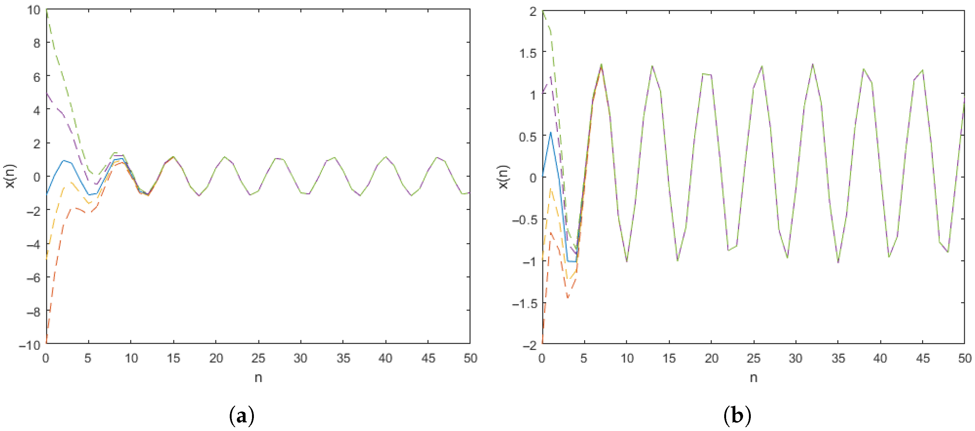
In this section, two examples, as well as their numerical simulations, are provided to illustrate our results.

Example 1.

The discrete Keynesian cross economic model was widely studied in [15,16,17]. This model with lagged income is given by

$$\left\{\begin{array}{c}D\left(n\right)=C\left(n\right)+I(n-1)+G(n-1)\hfill \\ C\left(n\right)=cx\left(n\right)\hfill \\ x(n+1)=\delta D(n+1)+(1-\delta )x\left(n\right),\hfill \end{array}\right.$$

where $c\ge 0$ is a constant, $D\left(n\right)$ is aggregate demand, $x\left(n\right)$ is aggregate income, $C\left(n\right)$ is aggregate consumption, $I\left(n\right)$ is aggregate investment, $G\left(n\right)$ is government spending, and $\delta <1$ is speed of adjustment term. Let $\delta c\ne 1$, then one can obtain the implicit form of the model as

$$x(n+1)={\displaystyle \frac{1-\delta }{1-\delta c}}x\left(n\right)+{\displaystyle \frac{\delta }{1-\delta c}}(I\left(n\right)+G\left(n\right)).$$

(27)

Set

$$A={\displaystyle \frac{1-\delta }{1-\delta c}},f\left(n\right)={\displaystyle \frac{\delta }{1-\delta c}}(I\left(n\right)+G\left(n\right)).$$

Let $\delta >0,c<1$, $I\left(n\right)$ and $G\left(n\right)$ be jointly quasi-periodic sequences. Then $A\in (0,1)$ satisfies the exponentially stability condition, and $f\left(n\right)={\displaystyle \frac{\delta }{1-\delta c}}(I\left(n\right)+G\left(n\right))$ is quasi-periodic. It follows from Theorem 1 that system (27) admits a unique bounded solution which is given by

$$x\left(n\right)=\sum _{i=-\infty }^{n-1}{({\displaystyle \frac{1-\delta }{1-\delta c}})}^{n-1-i}{\displaystyle \frac{\delta }{1-\delta c}}(I\left(i\right)+G\left(i\right)).$$

Moreover, by Theorem 2, this unique bounded solution is quasi-periodic and exponentially attracts any other solutions of Equation (27).

We perform numerical calculations via matlab for the case $\delta ={\displaystyle \frac{3}{5}},c={\displaystyle \frac{2}{3}}$ and $I\left(n\right)+G\left(n\right)=sinn$ (Figure 1a).

Example 2.

The following biological system models a single artificial effective neuron by dissipation and has been widely studied in [18,19,20]. The model is given by

$$x(n+1)=ax\left(n\right)+b\left(n\right)tanh\left(x\right(n\left)\right)+c\left(n\right),n\in \mathbb{Z}.$$

(28)

Set

$$A=a,F(n,x)=b\left(n\right)tanh\left(x\right(n\left)\right)+c\left(n\right).$$

Let $a\in (0,1)$, $b\left(n\right)$ and $c\left(n\right)$ be jointly Bohr almost periodic sequences with $\left|b\right(n\left)\right|<1-a$ for all $n\in \mathbb{Z}$. Then, the system (28) can be written as a discrete system of the form (9). It follows from Theorem 3 that the Equation (28) admits a unique bounded solution given by

$$x(n+1)=\sum _{i=\infty }^{n-1}{a}^{n-1-i}(b\left(i\right)tanhx\left(i\right)+c\left(i\right)),$$

which exponentially attracts every other solution of Equation (28). Furthermore, by Theorem 4, the unique bounded solution is Bohr almost periodic.

We perform numerical calculations via matlab for the case $a={\displaystyle \frac{1}{2}},b\left(n\right)={\displaystyle \frac{sinn}{4}},c\left(n\right)=cosn$ (Figure 1b).

Figure 1. (a) The numerical calculation for the case $\delta ={\displaystyle \frac{3}{5}},c={\displaystyle \frac{2}{3}}$ and $I\left(n\right)+G\left(n\right)=sinn$; (b) The numerical calculation for the case $a={\displaystyle \frac{1}{2}},b\left(n\right)={\displaystyle \frac{sinn}{4}},c\left(n\right)=cosn$.

Figure 1. (a) The numerical calculation for the case $\delta ={\displaystyle \frac{3}{5}},c={\displaystyle \frac{2}{3}}$ and $I\left(n\right)+G\left(n\right)=sinn$; (b) The numerical calculation for the case $a={\displaystyle \frac{1}{2}},b\left(n\right)={\displaystyle \frac{sinn}{4}},c\left(n\right)=cosn$.

References

1. Shcherbakov, B.A. Topologic Dynamics and Poisson Stability of Solutions of Differential Equations; Shtiintsa: Kishinev, Moldova, 1972. [Google Scholar]
2. Shcherbakov, B.A. The comparability of the motions of dynamical systems with regard to the nature of their recurrence. Differ. Equ. 1975, 11, 1246–1255. [Google Scholar]
3. Shcherbakov, B.A. Poisson Stability of Motions of Dynamical Systems and Solutions of Differential Equations; Stiinta: Chisinau, Moldova, 1985. [Google Scholar]
4. Shcherbakov, B.A.; Cheban, D. Asymptotically Poisson stable motions of dynamical systems and comparability of their reccurence in limit. Differ. Equ. 1977, 13, 898–906. [Google Scholar]
5. Caraballo, T.; Cheban, D. Almost periodic and almost automorphic solutions of linear differential/difference equations without Favard’s separation condition. I. J. Differ. Equ. 2009, 246, 108–128. [Google Scholar] [CrossRef]
6. Caraballo, T.; Cheban, D. Almost periodic and almost automorphic solutions of linear differential/difference equations without Favard’s separation condition. II. J. Differ. Equ. 2009, 246, 1164–1186. [Google Scholar] [CrossRef][Green Version]
7. Caraballo, T.; Cheban, D. Levitan/Bohr almost periodic and almost automorphic solutions of second order monotone differential equations. J. Differ. Equ. 2011, 251, 708–727. [Google Scholar] [CrossRef]
8. Caraballo, T.; Cheban, D. Almost periodic and almost automorphic solutions of linear differential equations. Dyn. Syst. 2010, 33, 1857–1882. [Google Scholar] [CrossRef]
9. Cheban, D. Levitan almost periodic and almost automorphic solutions of V-monotone differential equations. J. Dyn. Differ. Equ. 2008, 20, 669–697. [Google Scholar] [CrossRef]
10. Cheban, D.; Schmalfuss, B. Invariant manifolds, global attractors, almost automorphic and almost periodic solutions of non-autonomous differential equations. J. Math. Anal. Appl. 2008, 340, 374–393. [Google Scholar] [CrossRef][Green Version]
11. Cheban, D.; Liu, Z. Periodic, quasi-periodic, almost periodic, almost automorphic, Birkhoff recurrent and Poisson stable solutions for stochastic differential equations. J. Differ. Equ. 2020, 269, 3652–3685. [Google Scholar] [CrossRef]
12. Cheban, D.; Liu, Z. The comparability of motions in dynamical systems and recurrent solutions of (S)PDEs. Bul. Acad. Ştiinţe Republicii Mold. Mat. 2024, 104, 53–83. [Google Scholar] [CrossRef]
13. Sell, G.R. Lectures on Topological Dynamics and Differential Equations; Van Nostrand Reinhold Company: London, UK, 1971. [Google Scholar]
14. Sibirsky, K.S. Introduction to Topological Dynamics; Springer: Berlin/Heidelberg, Germany, 1975. [Google Scholar]
15. Ferguson, B.; Lim, G. Discrete Time Dynamic Economic Models: Theory and Empirical Applications; Routledge: Oxfordshire, UK, 2003. [Google Scholar]
16. Lizama, C.; Mesquita, J. Almost automorphic solutions of dynamic equations on time scales. J. Funct. Anal. 2013, 265, 2267–2311. [Google Scholar] [CrossRef]
17. Tisdell, C.; Zaidi, A. Basic qualitative and quantitative results for solutions to nonlinear, dynamic equations on time scales with an application to economic modelling. Nonlinear Anal. Theory Methods Appl. 2008, 68, 3504–3524. [Google Scholar] [CrossRef]
18. Fan, M.; Ye, D. Convergence dynamics and pseudo almost periodicity of a class of nonautonomous RFDEs with applications. J. Math. Anal. Appl. 2005, 309, 598–625. [Google Scholar] [CrossRef]
19. Gopalsamy, K.; Sariyasa, S. Time delays and stimulus dependent pattern formation in periodic environments in isolated neurons-II. Dyn. Contin. Discret. Impuls. Syst. Ser. B 2002, 9, 39–58. [Google Scholar]
20. Zhang, J.; Fan, M. Boundedness and stability of semi-linear dynamic equations on time scales. Prog. Qual. Anal. Funct. Equ. 2012, 1786, 45–56. [Google Scholar]
Disclaimer/Publisher’s Note: The statements, opinions and data contained in all publications are solely those of the individual author(s) and contributor(s) and not of MDPI and/or the editor(s). MDPI and/or the editor(s) disclaim responsibility for any injury to people or property resulting from any ideas, methods, instructions or products referred to in the content.