1. Introduction
Neural networks are a class of computational models inspired by biological nervous systems, processing and analyzing complex input data by simulating the connections and interactions between neurons in the human brain. Neural networks have shown great potential and value in various fields such as physical engineering [
1], biomedicine [
2], image processing [
3], associative memory [
4], pattern recognition [
5], and information security [
6], and have become a hot research topic. Recurrent neural networks have neurons interconnected in a closed-loop form, allowing information to flow and circulate continuously within the network. This structural characteristic makes it particularly suitable for handling complex interactions between multiple intelligent agents. When multiple intelligent agents are connected in a circular network, the circulation and sharing of information become very convenient, thereby significantly enhancing the collaborative efficiency and overall performance between agents [
7].
The concept of fractional calculus has a history of over three hundred years [
8]. Fractional calculus can be seen as a generalization of integer-order differentiation and integration, but due to the lack of application background, it has not attracted much attention for many years. With the deepening of research, fractional calculus has gradually become an active research direction [
9]. For example, the authors studied a nonlinear Volterra integro-differential equation with Caputo fractional derivative, multi-kernel and multi-constant delays, by defining appropriate Lyapunov functions and applying the Lyapunov–Razumikhin method, which not only provides a new way to study the qualitative properties of such equations, but also provides theoretical support for the stability analysis in practical applications [
10]. In recent years, many scholars have found that fractional calculus has a broad application prospect in the fields of science and engineering, and can effectively describe many complex phenomena, such as viscoelastic systems [
11], random diffusion [
12], dielectric polarization [
13], molecular spectroscopy [
14], and electromagnetic waves [
15]. Therefore, more and more practical systems can be accurately modeled through fractional integration and fractional differential equations, especially in describing materials and processes with infinite memory and hereditary characteristics, where fractional calculus shows more unique advantages than traditional integer-order calculus. Based on these advantages, the combination of fractional calculus and neural networks has also attracted widespread attention, as it can more accurately describe the dynamic characteristics of neural networks [
16].
Time delay refers to the phenomenon where the impact of changes in inputs or signals on the output of a dynamic system is subject to a certain time lag. Specifically, time delay reflects the response of a system or process lagging behind its input [
17]. In [
18], the authors outlined the dependence of stability type on time-delay characteristics and illustrated it with examples. Time delays are generally divided into leakage delays, self-connection delays, and communication delays. In neural networks, especially when dealing with time-series data [
19] and dynamic systems [
20], modeling and processing of time delays are crucial. Additionally, in a dynamic system, time delays are inevitable. Time delays can affect the stability of the system, leading to instability [
21], oscillations [
22], and chaos [
23], among other phenomena. Therefore, incorporating time delays in neural network models has significant practical importance.
Hopf bifurcation is an important phenomenon in nonlinear dynamics, describing the process by which a system transitions from a stable equilibrium point to periodic oscillations. Specifically, when one or more eigenvalues of a system shift from negative real numbers to complex numbers, the stability of the system changes, resulting in the creation of a limit cycle (i.e., a periodic solution). This type of bifurcation typically occurs when parameters change, marking a sudden change in system behavior, which can lead from a stable state to periodic oscillations, and even further into a chaotic state. Hopf bifurcation is widely applied in biology, engineering, and physics, such as in the fields of neural networks, ecological models, and oscillatory circuits [
24].
Quaternions were proposed by Irish mathematician William Rowan Hamilton in the mid-19th century. Quaternions are a number system that extends the concept of complex numbers, consisting of a real part and three imaginary parts, typically represented as
, where
a,
b,
c, and
d are real numbers, and
i,
j, and
k are imaginary units [
25]. Due to their higher dimension compared to real and complex numbers, quaternion neural networks can more naturally handle multi-dimensional data and the processing of high-dimensional signals. In three-dimensional space, quaternions can represent rotations and transformations more efficiently, making them significantly useful in neural networks that involve three-dimensional motion, physical modeling, or other complex multi-dimensional data [
26].
Based on the above analysis, this study will investigate the stability and Hopf bifurcation of fractional-order quaternion-valued cyclic neural networks with time delays. In summary, the research on fractional-order four-numerical cyclic neural networks involving time delays mainly focuses on these two aspects: (1) the existence, uniqueness, and boundedness of solutions for cyclic neural networks with multiple delays are studied; (2) as well as the stability and Hopf bifurcation of cyclic neural networks with multiple delays.
In [
27], the authors study the stability and bifurcation properties of the following integer-order quaternion-valued neural network:
where
are the states of neurons at time
t.
is a communication delay.
is a leakage delay.
is the self-regulating parameter of the neurons
.
are the interconnection coefficients.
are the neuron activation functions. The authors use matrix block theory to reduce the order of the characteristic equation. At the same time, taking the leakage delay and the communication delay as the bifurcation parameters, several conditions guaranteeing the stability of the periodic solution of Hopf bifurcation are established.
Inspired by the above analysis and based on the previous neural network model, we establish the following fractional-order quaternion-valued neural network involving delay:
where
is the real number,
represent the states of neurons at time
t,
denotes the set of quaternion number,
is the self-regulating parameter of the neurons
,
is a leakage delay,
is a communication delay.
denotes the connection weight between two neurons,
stands for the quaternion-valued activation function between two neurons.
The initial condition of system (
2) is prepared as follows:
where
,
is a constant and
.
The main contributions of this paper are as follows: (a) The formulated fractional-order delayed four-numerical neural network is decomposed into an equivalent real-valued system using the Cayley–Dickson construction. (b) The characteristic equation is a higher-order transcendental equation. Exploring the distribution of the roots of the characteristic equation is a challenge. We have solved this problem via the Coates’s flow-graph formula. (c) A new delay-independent stability and bifurcation criterion is presented. (d) The exploration method of bifurcations can be used to deal with many bifurcation problems for many fractional dynamical models. The remainder of the paper is shown below: In
Section 2, we give the basic definition of fractional calculus, lemma, and basic knowledge of quaternion. In
Section 3, we prove the existence and uniqueness of the solution of system (
2). In
Section 4, we check that the solution of the system (
2) is bounded. In
Section 5, we analyze the stability characteristics and Hopf bifurcation of system (
2). In
Section 6, we use software to perform numerical simulations to verify the correctness of the theoretical derivation. In
Section 7, the main conclusions of this paper are given.
2. Preliminaries
In this section, we outline the key definitions and lemmas of fractional calculus and the operations of quaternion algebra. These will be used in the proofs that follow. Due to the many advantages of Caputo derivatives, including the homogeneity of given initial conditions with integer-order derivatives, the description of physical properties, and the stronger applicability to real-world problems. In this paper, the Caputo derivative is used and the Caputo fractional differential is replaced by . Let denote the set of reals, denote the set of all nonnegative reals, and denote the set of quaternion.
Definition 1 ([
28])
. The Caputo fractional differential is defined as follows:where , , .The Laplace transform of the Caputo fractional-order derivatives iswhere . In particular, when the initial conditions , the above equation reduces to . Definition 2 ([
29])
. The Caputo fractional non-autonomous system with initial condition is defined as follows:where , is piecewise continuous with respect to and locally Lipschitz with respect to , is a domain with containing the origin . is the equilibrium point of system (4) if and only if . Lemma 1 ([
30])
. If the real-valued continuous function in system (4) satisfies the locally Lipschitz condition with respect to , then there exists a unique and continuous solution on . Lemma 2 ([
31])
. Assume that is a continuous function on , which satisfieswhere . Then,where is one-parameter Mittag-Leffler function. Therefore, the function is uniformly bounded on . Lemma 3 ([
32])
. Given the following n-dimensional linear fractional-order system with multiple delayswhere , the initial values . The characteristic matrix isif all the roots of have negative real parts, then the zero solution of system (5) is Lyapunov globally asymptotically stable. Lemma 4 ([
33])
. Let be the equilibrium point of system(2) and ρ be the eigenvalue of . Provided that , then is locally asymptotically stable. The quaternion [
34] is associative algebras defined on
, and the quaternion
x can be expressed as
where
,
i,
j,
k are all imaginary units of orthogonal unit vectors, and the imaginary units
i,
j,
k satisfy the following Hamilton rules:
From Hamilton rules, we can know the non-commutativity of quaternion multiplication. Suppose the quaternion
x,
y are labeled
,
, then, the addition, subtraction, and product operations of quaternion can be defined as
Define the conjugate of the quaternion
x as follows:
Define the norm of the quaternion
x as follows:
Define the reciprocal of quaternion
x as follows:
Using the Cayley–Dickson construction [
35], there is
set
is the plural of collection. For any quaternion
x, we have
where
,
, so we can obtain
According to the Cayley–Dickson structure, system (
2) can be transformed into the following six-dimensional equivalent system:
and the initial condition of system (
6) becomes
where
, when
,
is denoted as
n; when
,
is denoted as 1.
To arrive at the main conclusions of this study, we base our findings on the following reasonable necessary assumptions:
Assumption 1. Set . So, the quaternion numerical activation function is of the formThe functions , , , and with respect to exist and are continuous, and satisfy Assumption 2. There exist constants , such thatfor any , . Assumption 3. There exist constants , such that 5. Stability of the System and Hopf Bifurcation
In this part, we will explore the stability and bifurcation point of model (
6). For convenience, we will take the special case of
to provide some analytical results. When
the model is
Remark 1. Although three-dimensional dynamical systems have unique characteristics, they can effectively represent the core dynamical behavior of higher-dimensional systems. According to the Poincaré–Bendixson theorem, chaos cannot occur in two-dimensional continuous systems, but chaotic behavior can be observed in three-dimensional systems, such as the Lorenz attractor. This complexity is a hallmark of high-dimensional systems, making three dimensions a key dimension for studying phenomena like bifurcations and strange attractors. By studying the three-dimensional case, a universal analytical framework can be developed to understand general phenomena such as chaos, stability, and bifurcations, laying the groundwork for exploring the complexity of even higher-dimensional systems. The research on three-dimensional dynamical systems holds a unique and crucial position in the theory of dynamical systems. Despite its phase space dimensionality falling between low and high dimensions, this dimensionality both breaks through the limitations of two-dimensional systems and sufficiently reveals the general characteristics of high-dimensional systems, serving as a bridge for understanding complex dynamical behaviors.
Suppose that
in model (
10), and firstly verify the stability of system (
10) with leakage delay as a bifurcation parameter. According to Assumption 1, it is easy to determine that system (
10) has a unique equilibrium, which is the origin. The linear system of (
10) around the origin can be expressed as
where
The characteristic equation of system (
11) is
Equation (
12) is equivalent to the following form:
where
,
,
,
,
,
.
,
,
,
,
are defined by
Appendix A.
Multiply both sides of Equation (
13) by
to obtain
Assuming
in Equation (
14), then we have
Since
is constant, all roots
in Equation (
15) can be determined.
Denote the six roots of Equation (
15) by
where
,
are the real and imaginary parts of
, respectively.
Therefore, we can obtain
Assume that
is a purely imaginary root of Equation (
16). By substituting it into Equation (
16), the real and imaginary components can then be extracted separately. It is possible to obtain
By solving Equation (
17), we can calculate
From
, Equation (
18) we can obtain
It is obtained by Equation (
19) that
To determine the key conclusions of this section, the following assumptions are essential.
Assumption 4. Equation (20) has no positive real roots. Assumption 5. There exists at least one positive real root of Equation (20). From Assumption 5, with the help of Equation (
18), it can be obtained that
System (
6)’s bifurcation point is defined as follows:
where
is defined by Equation (
21).
Next, we will discuss the stability of system (
6) when
. The following Lemma 5 can be obtained and defined:
Lemma 5. If holds true at , then system (6) is locally asymptotically stable, where the definition of is as given above. Proof. When
, the characteristic Equation (
13) can be rewritten as
If the condition
is satisfied, then it is evident that all roots
fulfil the condition
. According to Lemma 4, it is straightforward to conclude that when
, system (
6) is globally asymptotically stable. □
To identify the conditions under which a Hopf bifurcation takes place, we make the following necessary assumption:
Assumption 6. where are defined by Appendix B. Lemma 6. Assume that is the root of Equation (14) in the vicinity of , and satisfying , , then the following transversality condition holds:where and represent the bifurcation point and the critical frequency of system (6). Proof. Differentiating both sides of Equation (
13) with respect to
yields
Simplifying Equation (
23), we obtain
where
From Equation (
24), it can be inferred that
According to Assumption 6, we determine that the transversality condition holds. This concludes the proof of Lemma 6. □
According to Assumptions 1, 4 and 5, and Lemmas 3, 5 and 6 holding, the following theorem can be derived:
Theorem 3. For system (10), the following results hold: - (i)
If Assumptions 1 and 4 and Lemma 3 are satisfied, then the zero equilibrium point is global asymptotically stable for .
- (ii)
If Assumptions 1 and 5, and Lemmas 5 and 6 hold, then
- (a)
The zero equilibrium point is locally asymptotically stable for η.
- (b)
When , system (6) undergoes a Hopf bifurcation at the origin, that is, there is a periodic solution branch near that bifurcates from the zero equilibrium point.
Remark 2. In [25], the authors discussed Hopf bifurcation of neural networks of integer order. However, we are talking about Hopf bifurcations of fractional neural networks, and the corresponding characteristic equations are also complex to compute. To solve this problem, we use Cayley–Dickson construction to transform the system into an equivalent complex-valued system, and Coates’s flow-graph formula is used to solve the higher-order characteristic equations of the related linearized system. Moreover, these methods can be extended to the study of octonion neural networks. If there is no leakage delay, then system (
10) becomes
We utilize the previously established analytical method to examine the stability and bifurcation issues of system (
25) in the absence of leakage delay, treating the communication delay as the bifurcation parameter. Additionally, we derive the criteria that lead to bifurcation due to this delay. It is evident that, based on Assumption 1, the origin serves as the equilibrium point for system (
25). The linear representation of system (
25) at the origin is as follows:
where
(
;
) is defined by Equation (
11).
The corresponding characteristic equation for system (
26) is
Equation (
27) is equivalent to
where
are defined by
Appendix A.
Multiplying both sides of Equation (
28) by
yields
Assuming
in Equation (
29), then we have
Since
is constant, all roots
in Equation (
30) can be determined.
Denote the six roots of Equation (
30) as
where
and
represent the real and imaginary components of
, respectively.
Let
(
) represent a purely imaginary solution to Equation (
31). By substituting this expression into Equation (
31) and then isolating the real and imaginary components, we obtain
Upon resolving Equation (
32), it follows that
where
From
, Equation (
33) can be transformed into
Next, we will explore whether Equation (
34) has positive real roots.
Lemma 7. For Equation (34), the following conclusions are drawn: - (1)
When , Equation (34) does not have any positive real roots. - (2)
When , Equation (34) results in six positive real rootswhere .
Proof. (1) Let us assume that
It follows from
and
that
. From
, we have
. Therefore, there are no positive real roots of Equation (
34).
(2) From Equation (
36) we can obtain
and
For
, Equations (
37) and (
38) imply the existence of at least one positive real root for
.
According to Equation (
36), it is possible to derive
Observing the conditions
,
, and
, we deduce that
. Consequently,
exhibits a monotonic rise within the interval
. This indicates that the positive real root of the equation
is singular. Therefore, Equation (
34) yields six positive solutions. This leads to the conclusion stated in (2). We then proceed to identify the positive roots of
, as outlined in Equation (
35). With this, the proof of Lemma 7 is successfully concluded. □
On account of
, it is obvious that
The bifurcation point for system (
25) is defined as follows:
where
are defined by Equation (
39).
In order to identify the conditions under which Hopf bifurcation occurs, we introduce the following necessary assumption:
Assumption 7. where are defined by Appendix C. Lemma 8. Assume that is the root of Equation (28) in the vicinity of , and satisfying , and , then the following transversality condition holds:where and denote the the bifurcation point and critical frequency of system (25), respectively. Proof. Taking the derivative of both sides of Equation (
28) with respect to
, we obtain
Simplifying Equation (
40), we obtain
where
From Equation (
41), it can be inferred that
According to the Assumption 7, we conclude that the transverse condition is satisfied. Thus, the proof of Theorem 8 is completed. □
From the aforementioned analysis, along with Assumptions 1 and 7 and Lemmas 3, 5, 7 and 8, the following theorem can be concluded.
Theorem 4. The following conclusions can be drawn about system (25): - (i)
The zero equilibrium point is globally asymptotically stable for provided Assumption 1, Lemma 3, and the first conclusion in Lemma 7 are satisfied.
- (ii)
If Assumptions 1 and 7, Lemma 5, and the second conclusion in Lemmas 7 and 8 are satisfied, then
- (a)
The zero equilibrium point exhibits local asymptotic stability within the interval .
- (b)
When , system (25) undergoes a Hopf bifurcation at the origin, i.e., it bifurcates from a periodic solution branch at near the zero equilibrium point.
6. Numerical Simulation
In this part, we present numerical examples to illustrate the credibility of our theoretical findings. The results from our simulations are derived from the Adams–Bashforth–Moulton predictor–corrector method [
36], utilizing a step size of h = 0.01.
Consider the following FQVNNs:
where
,
,
,
,
,
,
,
.
One can readily deduce that model (
42) possesses a zero equilibrium point. Using Matlab to program according to the reasoning process in
Section 5, and inputting the data, the characteristic equation can be obtained:
By solving the characteristic (
43) roots, we obtain
,
,
,
,
, and
. We separate the real and imaginary parts in sequence and substitute them into Equation (
20) to verify Assumption 5. This allows us to determine the bifurcation frequency and bifurcation point. From the characteristic Equation (
43), we can obtain the value of
, and after calculation, we verify that
in Lemma 5. Then, we take the derivative of the characteristic equation with respect to tau, substitute the required data to verify that Assumption 6 holds, and thus Lemma 6 also holds.
Thus, the second conclusion of Theorem 3 is satisfied, and from Equation (
22), we obtain the bifurcation point
, which also can be given by
Figure 1. From
Figure 1, we can see that when
, the system is locally asymptotically stable at the zero equilibrium point. When
,
exhibits Hopf bifurcation. As
increases, the Hopf bifurcation of
shows a trend of inflection points and increasing amplitude.
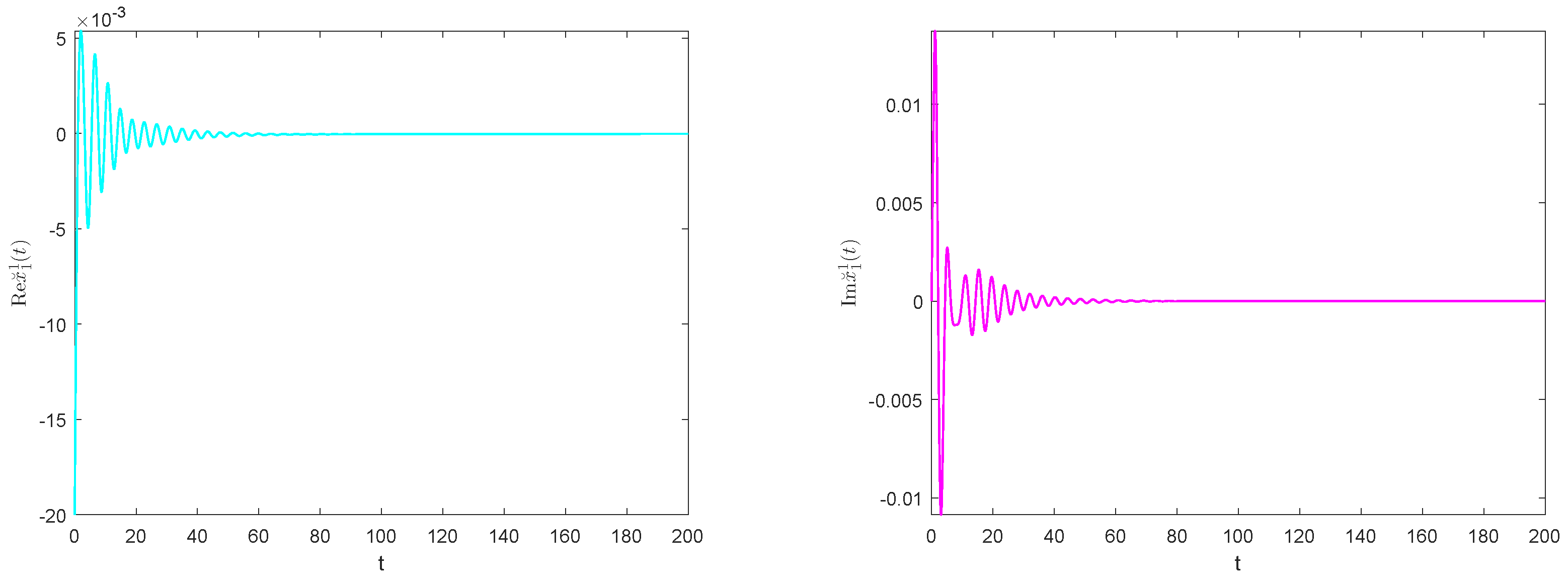
To better explain the conclusions obtained, we select
to perform numerical simulations, and plot the fluctuation diagrams and phase diagrams of all state variables of the system. To reduce the length of the paper, only the fluctuation diagrams and phase diagrams of the state variable
are provided in the text. The increasing fluctuations of the state variables
in
Figure 2 tend to stabilize over time, indicating that the system is locally asymptotic stable at the origin.
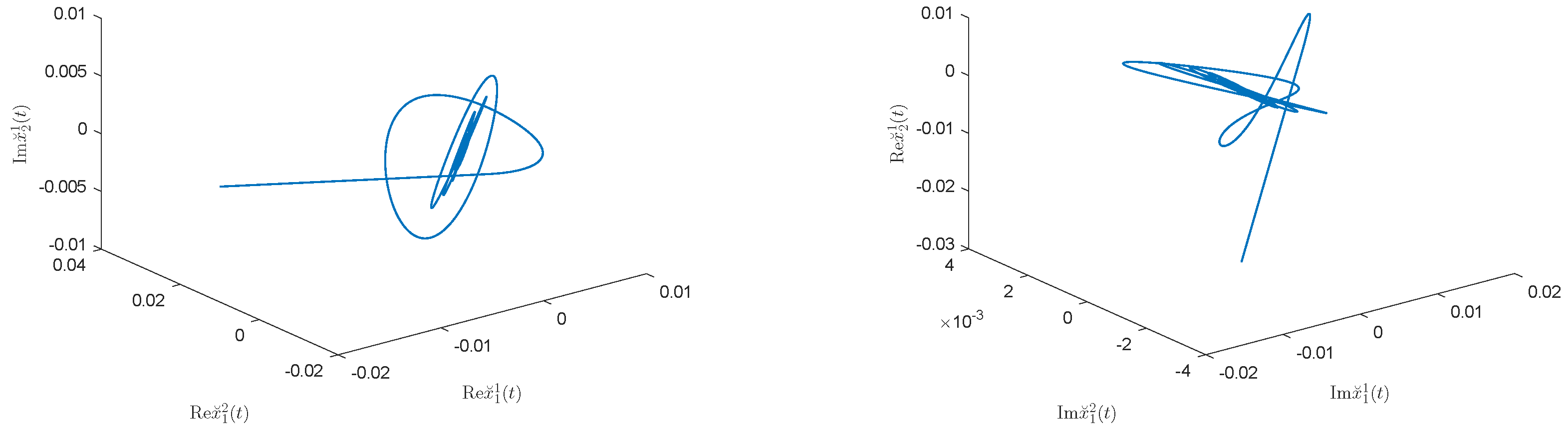
Figure 3 also demonstrates from the phase trajectory characteristics that the system is locally stable at the origin.
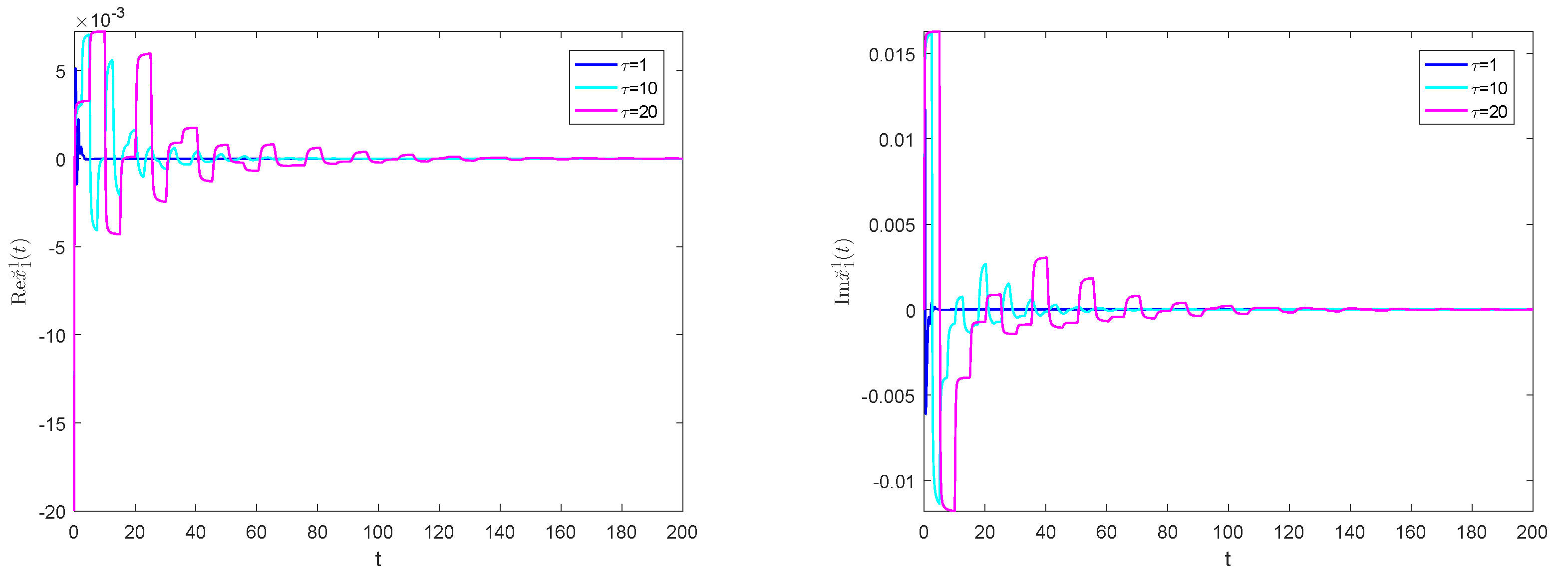
When
, the fluctuation rate of the state variables
at zero equilibrium point is shown in
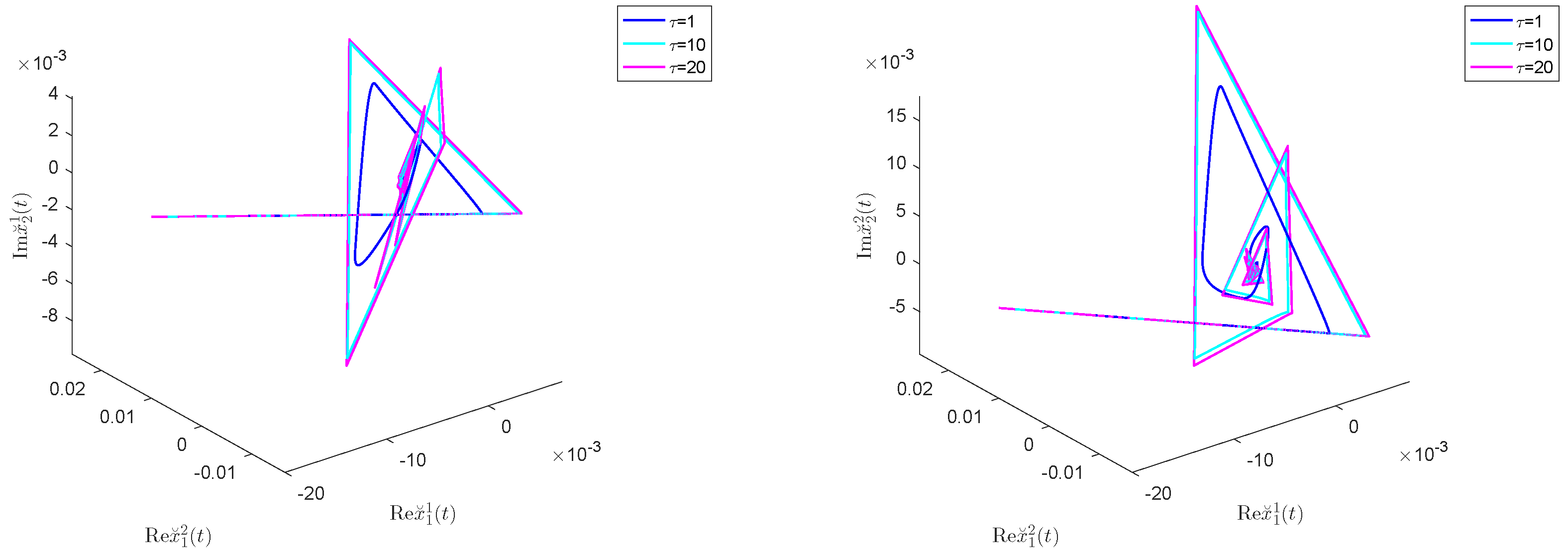
Figure 4, and the phase trajectory in
Figure 5 presents a complex ring structure, which indicates that the equilibrium point of the system becomes unstable and generates a limit cycle, which marks the occurrence of Hopf bifurcation in the system.
In addition, we studied how the order affects the bifurcation point; as shown in
Figure 6, the increase in the fractional order
leads to a corresponding increase in the bifurcation point value
, indicating that with the increase in the order, the emergence of Hopf bifurcation will cause the delay to appear.
Next, we discuss the bifurcation problem for the leakage-free delay system (
25). All parameters are sourced directly from system (
42) followed by
By substituting data into the derivation process of
Section 5, it is found that Equation (
34) has no positive real roots, thereby establishing the first conclusion of Lemma 7, and thus satisfying the first conclusion of Theorem 4. This implies that system (
44)’s zero equilibrium point has global asymptotic stability within the range of
.
We conducted numerical simulations with
and
, and plotted the fluctuation diagrams and phase diagrams of all state variables of system (
44). To reduce the length of the paper, only the fluctuation diagrams and phase diagrams of the state variable
are provided in the text.
Figure 7 shows that when
takes different values, the fluctuations of state variable
at the system (
44)’s zero equilibrium point become smoother as time is delayed.
Figure 8 also demonstrates that when
takes different values, the phase trajectory of state variable
at system (
44)’s zero equilibrium point gradually converges to 0, thus indicating that the system is globally asymptotically stable at the zero equilibrium point.


