A Comparison Index for Costs of Interval Linear Programming Models

Abstract

Interval Linear Programming (ILP) presents several compelling challenges when applied to real-world problems that cannot be easily captured by traditional robust uncertainty models. In this paper, we propose a novel solution method that employs a comparison index for interval ordering based on the generalized Hukuhara difference. This approach proves to be highly effective in comparing solutions within ILP frameworks. Additionally, we discuss the robustness of the proposed methodology and its implications for decision-making under uncertainty.

1. Introduction

The mathematical theory of linear programming models was established by Dantzig [1], where the coefficients of the objective function, constraint matrix, and right-hand sides of the constraints are assumed to be constant, meaning that uncertainty does not affect the description of a phenomenon. When uncertainty is unavoidable, as it happens in many real phenomena, it can be modeled in many robust ways, and in this paper, we adopt the replacement of constant coefficients with intervals of possible values (on the basis of Moore’s seminal book [2]).

In this paper, we propose a new efficient method to compare the objective solutions in Interval Linear Programming (ILP) that involve the comparison index introduced in two of our previous works ([3,4]) and are based on the generalized Hukuhara difference for intervals. We showed that the index summarizes the order relations proposed and analyzed by Ishibuchi and Tanaka in [5], where they consider the coefficients in mathematical programming problems as intervals and introduce five order relations for ranking two intervals; we provide evidence of the superiority of the comparison index in terms of errors and of worst-case loss in some optimization models. A complete characterization in several possible scenarios and the best and worst cases are described in [6], as well as the case of the inverse problem. We adopted the same comparison index in the research of the average rate of return for investment appraisal in uncertain conditions (see [7]).

The literature devoted to ILP is rich; here, we summarize some crucial contributions. Optimization problems in which the coefficients of the objective function and the constraints are interval numbers were investigated in a seminal paper by Tong in [8]: the interval of the solution is deduced by taking the maximum value range and minimum value range inequalities as constraint conditions. Sengupta and Pal, in [9], studied the same problem and proposed the concept of the acceptability index; see also reference [10] for an extended presentation of many contributions around the main theme.

One of the most exhaustive reviews of methods for solving ILP (Interval Linear Programming) problems with inequality constraints is presented in [11]. In [12], the optimal solution set of ILP is described as the intersection of regions arising from best and worst scenarios; in [13], the same authors introduce several methods for solving ILP problems when the primary model is transformed into two submodels, and in [14], they introduce an algorithm for large-scale problems based on the construction of the interval linear equation system that is the union of linear equations coming from the binding constraint indices of the optimal solution.

A second extended overview of the different approaches reported in the literature to deal with uncertainty in multiple objective linear models through interval programming can be found in [15], where the variety of approaches appears clearly; for example, in [16], a nonlinear interval programming problem is studied, converting the interval single-objective problem into a two-objective problem that considers both the average value and the robustness of the design, and in [17], the research of efficient solutions is highlighted within financial applications.

A unified scenario for optimal solutions is introduced in [18], where necessary and sufficient criteria for testing a class of optimality are developed according to the Karush–Kuhn–Tucker conditions; on the other hand, in [19], necessary conditions for efficiency in interval multi-objective linear programming are introduced, and in [20], the robustness of optimal solutions in terms of their capability to remain optimal when perturbations occur is studied. The contribution in [21] offers a different perspective within the ILP subject to interval constraints.

In [22], an ensemble framework for assessing solutions of interval programming problems is developed, where interval dominance rules are defined and their correlations are described via exclusion, inclusion, and equivalence. In addition, paper [23] deserves interest because set-type solution notions within ILP are defined using the Kulisch–Miranker order.

When interval uncertainty is extended to fuzzy uncertainty, we deal with fuzzy linear programming (FLP), which was born in 1970 with the seminal work on Decision Theory by Bellman and Zadeh ([24]); however, FLP problems were formally born in 1974 when Tanaka et al. ([25]) and Zimmermann ([26]) published their works modeling the set of constraints in linear programming as fuzzy sets. Ramík extensively worked on the topic and in [27] introduced a class of fuzzy optimization problems with objective function depending on fuzzy parameters; as a cornerstone of the research field, ref. [28] showed that FLP can tackle highly complex situations in an elegant and efficient way. More recently, a new method for solving fully fuzzy linear programming problems was presented in [29] in the case of inequality constraints and parameterized fuzzy numbers, by means of solving multi-objective linear programming problems. Previously, Arana-Jiménez, in [30], proposed an algorithm that does not use ranking functions to find the fuzzy optimal (non-dominated) solutions of fully fuzzy linear programming problems with inequality constraints, using triangular fuzzy numbers and not necessarily symmetric numbers, by solving a multi-objective linear problem with crisp numbers. More recently, a unique optimal solution for the linear programming problem was obtained in [31] through a lexicographic ranking-based solution methodology, and in [32], interval-valued fuzzy multi-objective linear programming enables the management of uncertain travel time.

This paper is organized as follows: After the Introduction, in the Section 2, we present preliminary properties necessary to compare interval numbers. Section 3 is devoted to the introduction of linear programming solutions, modeling costs through interval numbers. Numerical examples and sensitivity analyses are presented in Section 4, and Section 5 concludes the paper.

2. Preliminaries in Interval Number Comparison

An order relation for the ranking of interval numbers was introduced in [3], and it was then detailed in [4]. Basically, we need the following notation:

An interval $A=\left[a^{-},a^{+}\right]$ with $a^{-}\le a^{+}$ has a midpoint radius representation $A=\left(\widehat{a};\overline{a}\right)$ that is defined by the following values:

$$\widehat{a}={\displaystyle \frac{a^{+}+a^{-}}{2}},\overline{a}={\displaystyle \frac{a^{+}-a^{-}}{2}}$$

(1)

where $\overline{a}\ge 0$, such that

$$a^{-}=\widehat{a}-\overline{a},a^{+}=\widehat{a}+\overline{a}.$$

(2)

Canonical operations are defined in both notations:

$$A+B=\left[a^{-}+b^{-},a^{+}+b^{+}\right]=(\widehat{a}+\widehat{b};\overline{a}+\overline{b})$$

(3)

$$A-B=\left[a^{-}-b^{-},a^{+}-b^{+}\right]=(\widehat{a}-\widehat{b};\overline{a}-\overline{b})$$

(4)

And if $\lambda$ is a scalar, then

$$\lambda A=(\lambda \widehat{a};\left|\lambda \right|\overline{a}).$$

(5)

We also need the generalized Hukuhara difference (detailed in [33]), which is defined as

$$A{\ominus }_{gH}B=(\widehat{a}-\widehat{b};\left|\overline{a}-\overline{b}\right|)$$

(6)

in order to define the index for the interval number comparison.

Definition 1. 

Given two distinct intervals $A\ne B$, the gH-comparison index (of order 2) is defined as

$$CI(A,B)={\displaystyle \frac{\widehat{A{\ominus }_{gH}B}}{∥A{\ominus }_{gH}B∥}}$$

(7)

where $A{\ominus }_{gH}B$ is the gH-difference,

$$\forall A,B,\widehat{A{\ominus }_{gH}B}={\displaystyle \frac{{\left(A{\ominus }_{gH}B\right)}^{+}+{\left(A{\ominus }_{gH}B\right)}^{-}}{2}}$$

(8)

is the midpoint value, and

$${∥A{\ominus }_{gH}B∥}_2=\left({\left|\widehat{A{\ominus }_{gH}B}\right|}^2+{\overline{A{\ominus }_{gH}B}}^2\right)$$

(9)

is the Hausdorff distance.

A comparison index ratio can be defined when $\widehat{a}\ne \widehat{b}$ as

$${\gamma }_{A,B}={\displaystyle \frac{\overline{a}-\overline{b}}{\widehat{a}-\widehat{b}}}$$

(10)

and the relationship between the two indexes is

$$CI(A,B)={\displaystyle \frac{1}{\pm \sqrt{1+{\left({\gamma }_{A,B}\right)}^2}}}$$

(11)

where the sign + holds when $\widehat{a}>\widehat{b}$ and − when $\widehat{a}<\widehat{b}$.

Index ${\gamma }_{A,B}$ satisfies some properties as the invariance of scale and the invariance to interval translation.

In [4], we also show how it is possible to extend the definition of a comparison index to fuzzy intervals.

When comparing overlapping intervals $A=\left(\widehat{a},\overline{a}\right)$ and $B=(\widehat{b},\overline{b}),$ if the choice is based on midpoint values $\widehat{a}$ and $\widehat{b}$, then two kinds of risk arise (as pictured in Figure 1), and they can be focused on as follows.

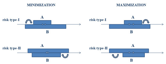
Figure 1. Type I and type II risks may occur in minimization and maximization problems.

Definition 2. 

A type I risk is defined to be the possible worst-case loss when, comparing A and $B,$ we choose A but there exist elements in B which are better than all elements of A.

Definition 3. 

A type II risk is defined to be the possible worst-case loss when, in comparing A and $B,$ we choose B but there exist elements in A that are worse than all elements of B.

The defined value ${\gamma }_{A,B}$ enables the definition of a “risk” measure that is detailed in [4], and that we recall as follows:

In the case of a minimization problem, we have a preliminary preference for A against B if $\widehat{a}<\widehat{b}$ (for the moment $\widehat{a}\ne \widehat{b}$) because the difference $\widehat{b}-\widehat{a}>0$ represents the midpoint gain if we choose A. On the other hand, taking into account the uncertainties given by $\overline{a}$ and $\overline{b}$, two possible bad situations may arise:

(i)

$b^{-}<a^{-}$, i.e., $\widehat{b}-\widehat{a}<\overline{b}-\overline{a}$, and this means that there exist values $b\in B$ such that $b<a$ for all $a\in A$;

(ii)

$a^{+}>b^{+}$, i.e., $\overline{b}-\overline{a}<\widehat{a}-\widehat{b}$, and this means that there exist values $a\in A$ such that $a>b$ for all $b\in B$.

In case (i), the positive quantity ${\displaystyle \frac{a^{-}-b^{-}}{\widehat{b}-\widehat{a}}}={\gamma }_{A,B}-1$ measures the possible regret, relative to the midpoint gain; in case (ii), a measure of the possible regret is given by the positive quantity ${\displaystyle \frac{a^{+}-b^{+}}{\widehat{b}-\widehat{a}}}=-{\gamma }_{A,B}-1$.

In terms of the the comparison index ratio ${\gamma }_{A,B}$, the relative regret measure is positive if ${\gamma }_{A,B}>1$ or if ${\gamma }_{A,B}<-1$, and the regret measures increase if ${\gamma }_{A,B}$ increases far from the threshold of 1 (case (i)) or decreases far from the threshold of $-1$ (case (ii)).

In the presence of worst-case loss for the two types of risk, value ${\gamma }_{A,B}$ can be limited by two fixed values ${\gamma }_m<0$ and ${\gamma }_M>0$ such that ${\gamma }_m\le {\gamma }_{A,B}\le {\gamma }_M$ and a new order relation can be introduced.

Definition 4. 

Given two intervals $A=\left[a^{-},a^{+}\right]=\left(\widehat{a};\overline{a}\right)$ and $B=\left[b^{-},b^{+}\right]=(\widehat{b};\overline{b})$, ${\gamma }_m<0$, and ${\gamma }_M>0$, we define the following (strict) order relation, denoted as ${<}_{{\gamma }_m,{\gamma }_M}$:

$$A{<}_{{\gamma }_m,{\gamma }_M}B⟺\left\{\begin{array}{c}\widehat{a}<\widehat{b}\\ {\gamma }_m\le {\gamma }_{A,B}\le {\gamma }_M\end{array}\right.⟺\left\{\begin{array}{c}\widehat{a}<\widehat{b}\\ {\gamma }_M\left(\widehat{a}-\widehat{b}\right)\le \overline{a}-\overline{b}\\ {\gamma }_m\left(\widehat{a}-\widehat{b}\right)\ge \overline{a}-\overline{b}\end{array}\right.$$

(12)

It can immediately be seen that the relation ${<}_{{\gamma }_m,{\gamma }_M}$ with ${\gamma }_m<0$, ${\gamma }_M>0$ is antisymmetric and transitive; furthermore, there are specific values of ${\gamma }_m$ and ${\gamma }_M$ that make the order relation (12) equivalent to the most cited order relations in the literature known with the acronyms of $LU,LC,UC,C{W}_M,$ and $C{W}_m$, as shown in the following definition.

Definition 5. 

$A\le {}_{LU}B\iff -1\le {\gamma }_{A,B}\le +1\iff a^{-}\le b^{-}$ and $a^{+}\le b^{+}$.

Let A and B be two intervals with $\widehat{a}<\widehat{b}$ and ${\gamma }_m\le {\gamma }_{A,B}\le$ ${\gamma }_M$. Then, it holds that

(1)

$A<{}_{LU}B⟺{\gamma }_{A,B}\in \left[-1,1\right]\Rightarrow {\gamma }_m=-1,{\gamma }_M=+1$;

(2)

$A<{}_{{CW}_M}B⟺{\gamma }_{A,B}\le 0\Rightarrow {\gamma }_m=-\infty ,{\gamma }_M=0$;

(3)

$A<{}_{{CW}_m}B⟺{\gamma }_{A,B}\ge 0\Rightarrow {\gamma }_m=0,{\gamma }_M=+\infty$;

(4)

$A<{}_{LC}B⟺{\gamma }_{A,B}\le 1\Rightarrow {\gamma }_m=-\infty ,{\gamma }_M=+1$;

(5)

$A<{}_{UC}B⟺{\gamma }_{A,B}\ge -1\Rightarrow {\gamma }_m=-1,{\gamma }_M=+\infty$.

By varying the two parameters ${\gamma }_m\le 0$ and ${\gamma }_M\ge 0$, we obtain a continuum of strict (partial) order relations for the interval. The set of real intervals $\mathbb{I}$ with the order relation ${\le }_{{\gamma }_m,{\gamma }_M}$ defined by $A{\le }_{{\gamma }_m,{\gamma }_M}B\iff (A{<}_{{\gamma }_m,{\gamma }_M}B$ or $A=B$) with ${\gamma }_m\le 0$ and ${\gamma }_M\ge 0$ is a complete lattice $(\mathbb{I},{\le }_{{\gamma }_m,{\gamma }_M})$.

Consequently, the decision-making midpoint representation can be defined as follows.

Definition 6. 

$A{\le }_{{\gamma }_m,{\gamma }_M}X\iff \left\{\begin{array}{c}\widehat{a}\le \widehat{x}\\ \overline{x}\le \widehat{a}+{\gamma }_M\left(\widehat{x}-\widehat{a}\right)\\ \overline{x}⩾\widehat{a}+{\gamma }_m\left(\widehat{x}-\widehat{a}\right)\end{array}\right.$

with $\widehat{x}\in R,\overline{x}\in R^{+}\cup \left\{0\right\}$.

For a given interval $A=(\widehat{a};\overline{a})$, consider the set of intervals represented in Figure 2:

$${\mathbb{D}}_{{\gamma }_m,{\gamma }_M}\left(A\right)\begin{array}{cc}=& \{X\in \mathbb{I}|A{\le }_{{\gamma }_m,{\gamma }_M}X\}\hfill \\ =& \left\{(\widehat{x};\overline{x})\right|\widehat{a}<\widehat{x}\mathrm{and}{\gamma }_m\le {\gamma }_{A,B}\le {\gamma }_M\}\cup \left\{(\widehat{a};\overline{a})\right\}.\hfill \end{array}$$

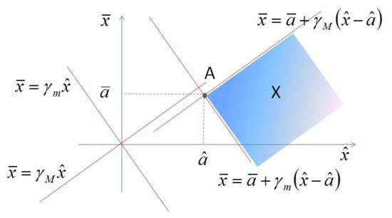
Figure 2. Visualization of the set of intervals ${\mathbb{D}}_{{\gamma }_m,{\gamma }_M}\left(A\right)$.

Proposition 1. 

For any real ${\gamma }_m<0$ and ${\gamma }_M>0$ (the slopes of the tangent lines) and any intervals $A,B\in \mathbb{I}$, we have

1.

$A{\le }_{{\gamma }_m,{\gamma }_M}B$ if and only if ${\mathbb{D}}_{{\gamma }_m,{\gamma }_M}\left(B\right)\subseteq {\mathbb{D}}_{{\gamma }_m,{\gamma }_M}\left(A\right)$;

2.

$A=B$ if and only if ${\mathbb{D}}_{{\gamma }_m,{\gamma }_M}\left(A\right)={\mathbb{D}}_{{\gamma }_m,{\gamma }_M}\left(B\right)$.

Given a family $\mathbb{A}=\left\{A_i\right|i\in \mathcal{I}\}$ of intervals (for any finite or infinite index set $\mathcal{I}$), the infimum and the supremum operators with respect to partial order ${\le }_{{\gamma }_m,{\gamma }_M}$, respectively, $C=\inf \{A\in \mathbb{A}\}$ and $D=\sup \{A\in \mathbb{A}\}$, are defined by the two intervals (in midpoint notation) $C=(\widehat{c};\overline{c})$ and $D=(\widehat{d};\overline{d})$:

$$\begin{array}{ccc}\hfill \widehat{c}& =& {\displaystyle \frac{{\gamma }_M{c}^{\prime }-{\gamma }_m{c}^{″}}{{\gamma }_M-{\gamma }_m}},\overline{c}={\displaystyle \frac{{\gamma }_M{\gamma }_m(c^{\prime }-c^{″})}{{\gamma }_M-{\gamma }_m}}\ge 0\hfill \\ \hfill \widehat{d}& =& {\displaystyle \frac{{\gamma }_M{d}^{\prime }-{\gamma }_m{d}^{″}}{{\gamma }_M-{\gamma }_m}},\overline{d}={\displaystyle \frac{{\gamma }_M{\gamma }_m(d^{\prime }-d^{″})}{{\gamma }_M-{\gamma }_m}}\ge 0\hfill \end{array}$$

(13)

where $c^{\prime }\le c^{″}$ are

$$\begin{array}{ccc}\hfill c^{\prime }& =& \inf \{\widehat{a}-{\displaystyle \frac{\overline{a}}{{\gamma }_M}}|A\in \mathbb{A}\}\hfill \\ \hfill c^{″}& =& \inf \{\widehat{a}-{\displaystyle \frac{\overline{a}}{{\gamma }_m}}|A\in \mathbb{A}\}\hfill \end{array}$$

(14)

and $d^{\prime }\le d^{″}$ are

$$\begin{array}{ccc}\hfill d^{\prime }& =& \sup \{\widehat{a}-{\displaystyle \frac{\overline{a}}{{\gamma }_M}}|A\in \mathbb{A}\}\hfill \\ \hfill d^{″}& =& \sup \{\widehat{a}-{\displaystyle \frac{\overline{a}}{{\gamma }_m}}|A\in \mathbb{A}\}.\hfill \end{array}$$

(15)

Remark 1. 

Focusing on an interval ordering index, we mention that the acceptability index for inequality $A<B$, introduced by Sengupta and Pal (see [9,10]) and defined by (assuming $\overline{a}+\overline{b}>0$)

$$Acc(A<B)={\displaystyle \frac{\widehat{b}-\widehat{a}}{\overline{a}+\overline{b}}},$$

(16)

is successfully used to convert an interval inequality $Ax\le B$, with $x\ge 0,$ into a “crisp equivalent” form as follows:

$$Ax{<}_{\alpha }B⟺\left\{\begin{array}{c}{a}^{+}x\le b^{+}\\ Acc(B<Ax)\ge \alpha \end{array}\right.$$

(17)

where $\alpha \in ]0,1]$ is an assumed fixed (optimistic) threshold. Substituting the expression for $Acc(B<Ax)$, we obtain

$$Ax{<}_{\alpha }B⟺\left\{\begin{array}{c}\widehat{a}x+\overline{a}x\le \widehat{b}+\overline{b}\\ \widehat{a}x-\alpha \overline{a}x\ge \widehat{b}+\alpha \overline{b}\end{array}\right..$$

(18)

This set of inequalities, being $\alpha >0$, implies that $\widehat{a}x\ge \widehat{b}+\alpha \overline{b}+\alpha \overline{a}x>\widehat{b}$ and does not imply control on the possible worse-case losses. In fact, we can see that $Ax{<}_{{\gamma }_m,{\gamma }_M}B$ is not equivalent to $Ax{<}_{\alpha }B$ in the sense that one cannot be transformed into the other.

The comparison index can be applied when a variable interval of the form $Ax$ is compared with a fixed interval B. two possible worst-case losses may occur, and they are related to the value of $\gamma$. Supposing $x\ge 0,$ it follows that the value of $\gamma$ for the inequality $Ax<B$ is

$${\gamma }_{Ax,B}={\displaystyle \frac{\overline{a}x-\overline{b}}{\widehat{a}x-\widehat{b}}}.$$

(19)

In order to control the extent of the possible worst-case loss for the two types of risk, we can require that the value ${\gamma }_{Ax,B}$ be controlled for the type I risk and/or for the type II risk. To do this, we fix two values ${\gamma }_m<0$ and ${\gamma }_M>0$, and we require that valid values of x satisfy $\widehat{a}x<\widehat{b}$ and ${\gamma }_m\le {\gamma }_{Ax,B}\le {\gamma }_M.$

The two types of risk are eliminated when ${\gamma }_m$$\in \left[-1,0\right]$ and ${\gamma }_M$$\in \left[0,1\right].$ The values $1-{\gamma }_M$ and $1+{\gamma }_m$, if negative, give the relative worst-case loss with respect to $\widehat{a}x-\widehat{b}$.

In terms of (12), we can write:

$$Ax{<}_{{\gamma }_m,{\gamma }_M}B⟺\left\{\begin{array}{c}\widehat{a}x<\widehat{b}\\ {\gamma }_M\widehat{a}x-\overline{a}x\le {\gamma }_M\widehat{b}-\overline{b}\\ {\gamma }_m\widehat{a}x-\overline{a}x\ge {\gamma }_m\widehat{b}-\overline{b}\end{array}\right..$$

(20)

If we are minimizing and we do not accept a risk of type II, we may require that $1+{\gamma }_{Ax,B}\ge 0$ (we eventually accept only a risk of type I), and we choose ${\gamma }_m=-1$, ${\gamma }_M=BIG>0$; a risk of type II represents the possibility that we have values in $Ax$ that are greater than all values in B. Similarly, if we do not accept a risk of type I, then we choose ${\gamma }_M=1$, ${\gamma }_m=-BIG<0$; a risk of type I represents the possibility that we have values in B that are less than all values in $Ax$. If ${\gamma }_m=-1$ and ${\gamma }_M=1$, no risk of the two types is accepted. It follows that the use of the acceptability index does not avoid the two types of risk that are controlled using the order relationship (12).

3. New Approach for Linear Programming with Interval Costs

The order relation ${\le }_{{\gamma }_m,{\gamma }_M}$ allows for the introduction of an innovative method in the search of a solution to the problem of linear programming with interval costs (ILP problem) that has the following general form:

$$\begin{array}{ccc}\hfill \min z\left(\underline{x}\right)& =& \left[z^{-}\left(x\right),z^{+}\left(x\right)\right]=(\widehat{z}\left(x\right);\overline{z}\left(x\right))\hfill \end{array}$$

(21)

$$\begin{array}{ccc}\hfill \widehat{z}\left(x\right)& =& \sum _{j=1}^n{\widehat{c}}_j{x}_j\overline{z}\left(x\right)=\sum _{j=1}^n{\overline{c}}_j{x}_j\hfill \\ \hfill s.t.{\left(Ax\right)}_j& \le & b_{i}i=1,\dots ,mA=\left[a_{i,j}\right]\in {\mathbb{R}}^{m\times n}{x}_j\ge 0j=1,\dots ,n\hfill \end{array}$$

(22)

where A is a matrix with m rows and n columns, b is an m-vector of right-hand-side terms, $c_j=({\widehat{c}}_j;{\overline{c}}_j)$, and $j=1,2,\dots ,n$ are n intervals representing the coefficients of the linear objective function $z\left(x\right)$ to be minimized, which is represented by an interval

$$z\left(x\right)=\left[z^{-}\left(x\right),z^{+}\left(x\right)\right]=(\widehat{z}\left(x\right);\overline{z}\left(x\right))$$

(23)

where $\widehat{z}\left(x\right)$ and $\overline{z}\left(x\right)$ are given by

$$\begin{array}{ccc}\hfill \widehat{z}\left(x\right)& =& \sum _{j=1}^n{\widehat{c}}_j{x}_j\hfill \\ \hfill \overline{z}\left(x\right)& =& \sum _{j=1}^n{\overline{c}}_j{x}_j\hfill \end{array}$$

(24)

An optimal solution $x^{*}$ is computed with the corresponding objective value: ${\widehat{z}}_{\min }={\displaystyle \sum _{j=1}^n}{\widehat{c}}_j{x}_j^{*}$, where x is in the feasible convex set of

$$\mathbb{X}=\left\{x\in {\mathbb{R}}^n|x\ge 0,Ax\le b\right\}.$$

(25)

and the set of feasible objective intervals is again a convex set:

$$\mathbb{Z}=\left\{z\left(x\right)\in \mathbb{I}|x\in \mathbb{X}\right\}$$

Remark 2. 

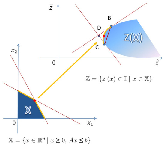
It is well known that $\mathbb{X}$ is a convex polygon in ${\mathbb{R}}^n$, and this implies that $\mathbb{Z}$ is a convex polygon in the space $\mathbb{I}$ of intervals, as shown in Figure 3.

Figure 3. Visualization of the process from the feasible convex set to the feasible objective intervals.

Definition 7. 

If $x^{\prime },x^{″}\in \mathbb{X}$ are two feasible solutions and $z^{\prime }=\left({\widehat{z}}^{\prime };{\overline{z}}^{\prime }\right),z^{″}=\left({\widehat{z}}^{″};{\overline{z}}^{″}\right)$ are the corresponding objective interval values, then $x^{\prime }$ dominates $x^{″}$ (or in other words, $z^{\prime }$ dominates $z^{″})$ if and only if $z^{″}{<}_{{\gamma }_m,{\gamma }_M}{z}^{″}.$

The search of a solution $x\in \mathbb{X}$ requires the following method: among all the feasible objective values, the non-dominated values, with respect to the interval relation order ${<}_{{\gamma }_m,{\gamma }_M}$(with fixed ${\gamma }_m<0$, ${\gamma }_M>0$) have to be selected. In particular, given two feasible solutions $x^{\prime }$ and $x^{″}$, with the corresponding objective intervals given by $z^{\prime }=\left({\widehat{z}}^{\prime },{\overline{z}}^{\prime }\right)$ and $z^{″}=\left({\widehat{z}}^{″},{\overline{z}}^{″}\right)$, the problem involves choosing the best interval between them. Three possible situations may occur.

Given two feasible solutions $x^{\prime }$ and $x^{″}$ with the corresponding objective intervals given by $z^{\prime }=\left({\widehat{z}}^{\prime },{\overline{z}}^{\prime }\right)$ and $z^{″}=\left({\widehat{z}}^{″},{\overline{z}}^{″}\right),$ the best interval between them corresponds to three cases:

• $x^{\prime }$ is better than (dominates)$x^{″}$ or equivalently $z^{\prime }{\le }_{{\gamma }_m,{\gamma }_M}{z}^{″};$
• $x^{″}$ is better than (dominates)$x^{\prime }$ or equivalently $z^{″}{\le }_{{\gamma }_m,{\gamma }_M}{z}^{\prime };$
• $x^{\prime }$ and $x^{″}$ are not comparable because of the incomparability between $z^{\prime }$ and $z^{″}.$

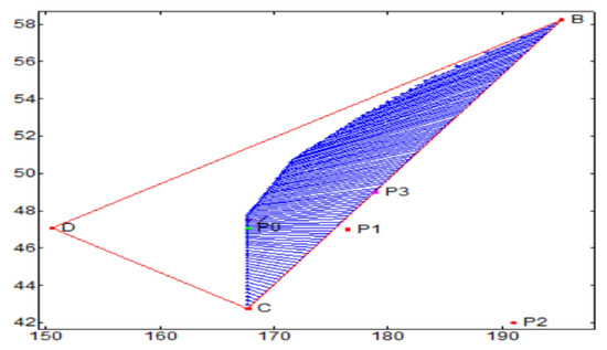
Consequently, a solution x is called efficient if there is no feasible solution $x^{\prime }$ such that $x^{\prime }$ dominates x. It follows that, as shown in Figure 4, the lines tangent to $\mathbb{Z}$ determine the ideal objective interval that has values between the tangent points called $P=\left(\widehat{p},\overline{p}\right)$ and $Q=\left(\widehat{q},\overline{q}\right)$. Here, we want the ideal objective solution to be the best possible solution for each objective function in a multi-objective optimization problem; at the ideal point, all objectives are simultaneously optimized even if it is not achievable or feasible.

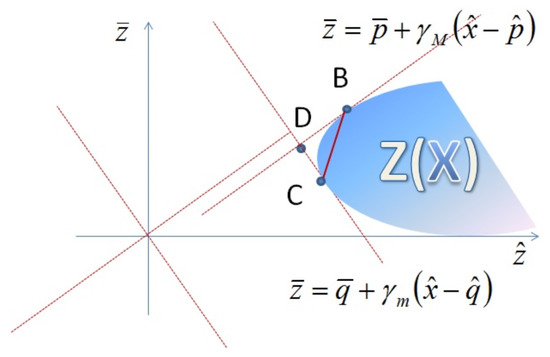
Figure 4. Representation of lines tangent to $\mathbb{Z}$.

The main interpretation of the expression $z\left(x^{\prime }\right){\le }_{{\gamma }_m,{\gamma }_M}z\left(x^{″}\right)$ involves the following:

• $x^{\prime }$ dominates $x^{″}$ in the variable space X;
• $z\left(x^{\prime }\right)$ dominates $z\left(x^{″}\right)$ in the space of an interval object.

The DBC triangle construction provides two important pieces of information:

• The efficient boundary of the LP problem, in the target value space $\mathbb{Z}\left(\mathbb{X}\right)$$\left[z\left(x_1,x_2,\dots ,x_n\right)\in \mathbb{Z}\left(\mathbb{X}\right)\right]$, is inside triangle DBC.
• Value D identifies the ideal objective solution; it is unique in $\mathbb{Z}$, but not necessarily in $\mathbb{X}$ and this implies the following:
  $z_D=GLB\left(\mathbb{Z}\left(\mathbb{X}\right)\right)$ Greatest Lower Bounded with respect to ${\le }_{{\gamma }_m,{\gamma }_M}$;
  If $D\in \mathbb{Z}\left(\mathbb{X}\right)$, then D is unique and is the ideal solution.

The efficient frontier is determined by two “tangent” lines or better “support lines”:

(1)

$\overline{z}=\overline{p}+{\gamma }_M\left(\widehat{z}-\widehat{p}\right)$, where P is feasible, and $\widehat{p}=\widehat{z}\left(x_P\right)$ and $\overline{p}=\overline{z}\left(x_P\right)$ with $x_P\in \mathbb{X}$ such that $\overline{p}-{\gamma }_M\widehat{p}$ is the largest.

(2)

$\overline{z}=\overline{q}+{\gamma }_m\left(\widehat{z}-\widehat{q}\right)$ where Q is feasible, and $\widehat{q}=\widehat{z}\left(x_Q\right)$ and $\overline{q}=\overline{z}\left(x_Q\right)$ with $x_Q\in \mathbb{X}$ such that $\overline{q}-{\gamma }_m\widehat{q}$ is the smallest.

The intersection between tangent lines is the ideal solution $z_{id}=\left({\widehat{z}}_{id},{\overline{z}}_{id}\right):$

$$\left\{\begin{array}{c}\overline{z}=\overline{p}+{\gamma }_M\left(\widehat{z}-\widehat{p}\right)\\ \overline{z}=\overline{q}+{\gamma }_m\left(\widehat{z}-\widehat{q}\right)\end{array}\right.\left\{\begin{array}{c}{\widehat{z}}_{id}={\displaystyle \frac{\overline{q}-\overline{p}+{\gamma }_M\widehat{p}-{\gamma }_m\widehat{q}}{{\gamma }_M-{\gamma }_m}}\\ {\overline{z}}_{id}={\displaystyle \frac{{\gamma }_m\left({\gamma }_M\widehat{p}-\overline{p}\right)-{\gamma }_M\left({\gamma }_m\widehat{q}-\overline{q}\right)}{{\gamma }_M-{\gamma }_m}}\end{array}\right.$$

(26)

The interval-valued LP optimal solution has the following qualities:

• If $z_{id}\in \mathbb{Z}$ (it is feasible), then it is the unique optimal solution;
• If $z_{id}\notin \mathbb{Z}$ (it is not feasible), then a goal programming technique is applied in order to find the feasible solution $z^{*}=\left({\widehat{z}}^{*},{\overline{z}}^{*}\right)$ with the smallest distance to $z_{id}$, i.e., the optimal feasible solution that solves the following optimization problem:

$$\min {\left(\sum _{j=1}^n{\widehat{c}}_j{x}_j-{\widehat{z}}_{id}\right)}^2+{\left(\sum _{j=1}^n{\overline{c}}_j{x}_j-{\overline{z}}_{id}\right)}^2$$

(27)

$$\begin{array}{ccc}\hfill s.t.{\left(Ax\right)}_j& \le & b_{i}i=1,..,mA=\left[a_{i,j}\right]\in {\mathbb{R}}^{m\times n}\hfill \\ \hfill x_j& \ge & 0j=1,..,n\hfill \end{array}$$

A solution x is efficient if there is no feasible solution $x^{\prime }$ such that $x^{\prime }$ dominates x.

Tangent lines (support lines) to $\mathbb{Z}$ determine the ideal objective interval that has values between the tangent points called $P=\left(\widehat{p},\overline{p}\right)$ and $Q=\left(\widehat{q},\overline{q}\right).$

4. Numerical Examples and Sensitivity Analysis

To validate the robustness of our index, we show that, thanks to its use, it is possible to obtain more precise solutions in three linear programming problems with interval costs, two of which are well known in the literature; in this way, we extend preliminary results shown in [34] and refer to [35,36] for an exhaustive scenario of properties concerning the calculus of interval-valued functions.

Example 1. 

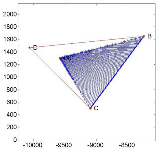
The first example explains the new methodology when data are specified in order to give an idea of the difference between the ideal solution and the optimal solution, as shown in Figure 5:

$$A=\left[\begin{array}{cc}1& 1\\ 4& 2\\ 2& 4\end{array}\right];b=\left[\begin{array}{c}40\\ 132\\ 140\end{array}\right]$$

$$\widehat{c}=\left[\begin{array}{c}-250\\ -220\end{array}\right];\overline{c}=\left[\begin{array}{c}50\\ 0\end{array}\right]$$

Figure 5. Ideal and optimal solutions of example 1 are shown.

The same figure shows that, given the feasible set, it is possible to identify the slopes ${\gamma }_m\le 0$ and ${\gamma }_M\ge 0$ of the two red tangent lines; after that, the third red line connects the tangent points. The area described by blue lines is the feasible set, and D is the ideal solution $z_{id}$ in (27) that does not belong to the feasible set and it requires the mentioned goal programming technique to identify the minimum value $P0$ as $z^{*}.$

The sensitivity analysis for the optimal solution is carried out through a graphic where values of the two variables x and y and their frequencies are shown in order to observe the robustness of the solution. The vertical and horizontal histograms in Figure 6 show the distribution of the values of x and y around the optimal solution.

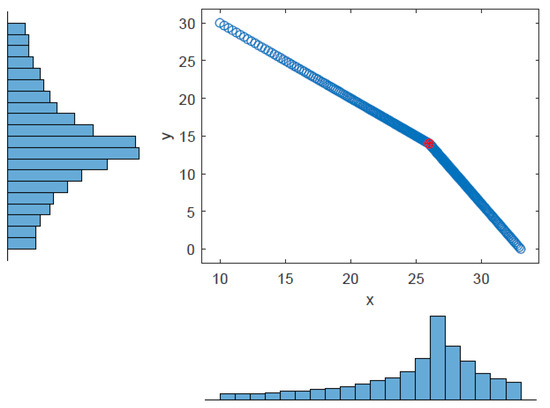
Figure 6. Sensitivity analysis for example 1.

Example 2. 

The second example is the same one described in [37] with interval coefficients in the objective function, where the optimization problem has the following expression, with $x_j\ge 0$ and $j=1,2$:

$$\max \left[-20,50\right]x_1+\left[0,10\right]x_2$$

$$s.t.\left[\begin{array}{cc}10& 60\\ 10& 20\\ 10& 10\\ 30& 10\\ 40& 10\end{array}\right]\left[\begin{array}{c}{x}_1\\ x2\end{array}\right]\le \left[\begin{array}{c}1080\\ 400\\ 240\\ 420\\ 520\end{array}\right]$$

We have solved the problem in the minimization form so that the midpoint values of the objective function are negative. Figure 7 shows the minimum value $P0$ obtained with the slope of the tangent lines specified by the values ${\gamma }_m=0$ and ${\gamma }_M=5$. Point $P1=\left(-90;90\right)$ is the minimum obtained in [37], and it is exactly the same as the one obtained with our method (as the nearest interval to the ideal solution $D,$ corresponding to the chosen values of ${\gamma }_m$ and ${\gamma }_M)$. The second solution suggested by Chanas and Kuchta is equal to $(-210;390)$, and it is presented in Figure 8, while the solution obtained with our method with the partial order generated by ${\gamma }_m=-2$ and ${\gamma }_M=1.5$ is clearly closer to D.

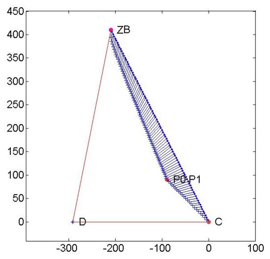
Figure 7. Numerical example n.2 (Chanas and Kuchta) with ${\gamma }_m=0$ and ${\gamma }_M=5.0$.

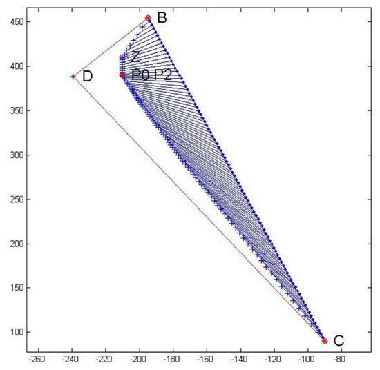
Figure 8. Numerical example n.2 (Chanas and Kuchta) with ${\gamma }_m=-2$ and ${\gamma }_M=1.5$.

In addition, the graphic representation that our methodology provides is particularly explanatory.

Example 3. 

The third numerical example is a problem called ITPMPF (Interval-valued Transportation Problem with Multiple Penalty Factors) that comes from chapter 7 of the book [10], and it is defined as

$$\begin{array}{ccc}\hfill \min Z^1& =& \sum _{i=1}^3\sum _{j=1}^4{c}_{ij}^1{x}_{ij}\hfill \end{array}$$

(28)

$$\min Z^2=\sum _{i=1}^3\sum _{j=1}^4{c}_{ij}^2{x}_{ij}$$

(29)

$$s.t.\sum _{j=1}^4{x}_{1j}=[7,9],\sum _{j=1}^4{x}_{2j}=[17,21],\sum _{j=1}^4{x}_{3j}=[16,18]$$

$$\begin{array}{ccc}\hfill \sum _{i=1}^3{x}_{i1}& =& [10,12],\sum _{i=1}^3{x}_{i2}=[2,4]\hfill \end{array}$$

(30)

$$\begin{array}{ccc}\hfill \sum _{i=1}^3{x}_{i3}& =& [13,15],\sum _{i=1}^3{x}_{i4}=[15,17]\hfill \\ \hfill x_j& \ge & 0i=1,2,3j=1,2,3,4\hfill \end{array}$$

(31)

where

$$C^1=\left(c_{ij}^1\right)=\begin{array}{cccc}\left[1,2\right]& \left[1,3\right]& \left[5,9\right]& \left[4,8\right]\\ \left[1,2\right]& \left[7,10\right]& \left[2,6\right]& \left[3,5\right]\\ \left[7,9\right]& \left[7,11\right]& \left[3,5\right]& \left[5,7\right]\end{array}$$

(32)

$$C^2=\left(c_{ij}^2\right)=\begin{array}{cccc}\left[3,5\right]& \left[2,6\right]& \left[2,4\right]& \left[1,5\right]\\ \left[4,6\right]& \left[7,9\right]& \left[7,10\right]& \left[9,11\right]\\ \left[4,8\right]& \left[1,3\right]& \left[3,6\right]& \left[1,2\right]\end{array}$$

We chose ${\gamma }_m=-0.25$ and ${\gamma }_M$$=0.25.$ In Figure 9, $P0=\left(167.75;47.0625\right)$ is the minimum obtained with our methodology, $P1=\left(176.5;47\right)$ and $P2=\left(191;42\right)$ are the minima obtained with the reduction into a standard LPP structure as in [10], and $P3=\left(178.875;48.985\right)$ is the solution of the same problem obtained in [38]. We remark that solutions $P1$, $P2$, and $P3$ are not on the efficient frontier of the feasible objective values.

Figure 9. Numerical example 3 (Sengupta and Pal).

The figure clearly shows that $P0$ is the closest to the ideal minimum D, and it demonstrates, also from the graphical point of view, the effectiveness of the methodology based on our comparison index also in a multivariable setting.

5. Further Directions and Conclusions

The introduction of the comparison index introduced in two of our previous works ([3,4]) allows for a significant improvement in finding solutions in Interval Linear Programming (ILP) problems compared to other established methodologies. Most importantly, the improvement of the new methodology has a very clear graphical representation that helps in the comprehension of the real problem.

The natural next step is to approach uncertainty by extending intervals to fuzzy numbers in order to also introduce the possibility of uncertain values and to define a more flexible methodology that can be very useful for real-world applications.

References

- Dantzig, G.B. Linear Programming and Extensions; Princeton University Press: Princeton, NJ, USA, 1963. [Google Scholar]
- Moore, R.E. Methods and Applications of Interval Analysis, Philadelphia; Society for Industrial and Applied Mathematics: Philadelphia, PA, USA, 1979. [Google Scholar]
- Guerra, M.L.; Stefanini, L. A comparison index for interval ordering. In Proceedings of the IEEE SSCI 2011, Symposium Series on Computational Intelligence (FOCI 2011), Paris, France, 11–15 April 2011; pp. 53–58. [Google Scholar]
- Guerra, M.L.; Stefanini, L. A comparison index for interval ordering based on generalized Hukuhara difference. Soft Comput. 2012, 16, 1931–1943. [Google Scholar] [CrossRef]
- Ishibuchi, H.; Tanaka, H. Multiobjective programming in optimization of the interval objective function. Eur. J. Oper. Res. 1990, 48, 219–225. [Google Scholar] [CrossRef]
- Mostafaee, A.; Hladík, M.; Černý, M. Inverse linear programming with interval coefficients. J. Comput. Appl. Math. 2016, 292, 591–608. [Google Scholar] [CrossRef]
- Guerra, M.L.; Magni, C.A.; Stefanini, L. Interval and fuzzy average internal Rate of Return for investment appraisal. Fuzzy Sets Syst. 2014, 257, 217–241. [Google Scholar] [CrossRef]
- Tong, S. Interval number, fuzzy number linear programming. Fuzzy Sets Syst. 1994, 66, 301–306. [Google Scholar] [CrossRef]
- Sengupta, A.; Pal, T.K. On comparing interval numbers. Eur. J. Oper. Res. 2000, 127, 28–43. [Google Scholar] [CrossRef]
- Sengupta, A.; Pal, T.K. Fuzzy Preference Ordering of Interval Numbers in Decision Problems; Springer: Berlin/Heidelberg, Germany, 2009. [Google Scholar]
- Allahdadi, M.; Nehi, H.M. The optimal solution set of the interval linear programming problems. Optim. Lett. 2013, 7, 1893–1911. [Google Scholar] [CrossRef]
- Allahdadi, M.; Nehi, H.M.; Ashayerinasab, H.A.; Javanmard, M. Improving the modified interval linear programming method by new techniques. Inf. Sci. 2016, 339, 224–236. [Google Scholar] [CrossRef]
- Nehi, H.M.; Ashayerinasab, H.A.; Allahdadi, M. Solving methods for interval linear programming problem: A review and an improved method. Oper. Res. Int. J. 2020, 20, 1205–1229. [Google Scholar] [CrossRef]
- Ashayerinasab, H.A.; Nehi, H.M.; Allahdadi, M. Solving the interval linear programming problem: A new algorithm for a general case. Expert Syst. Appl. 2018, 93, 39–49. [Google Scholar] [CrossRef]
- Oliveira, C.; Antunes, C.H. Multiple objective linear programming models with interval coefficients—An illustrated overview. Eur. J. Oper. Res. 2007, 181, 1434–1463. [Google Scholar] [CrossRef]
- Jiang, C.; Han, X.; Liu, G.R.; Liu, G.P. A nonlinear interval number programming method for uncertain optimization problems. Eur. Oper. Res. 2008, 188, 1–13. [Google Scholar] [CrossRef]
- Bata, A.; Allahdadi, M.; Hladík, M. Obtaining Efficient Solutions of Interval Multi-objective Linear Programming Problems. Int. J. Fuzzy Syst. 2020, 22, 873–890. [Google Scholar] [CrossRef]
- Li, H. Necessary and sufficient conditions for unified optimality of interval linear program in the general form. Linear Algebr. Its Appl. 2015, 484, 154–174. [Google Scholar] [CrossRef]
- Hladík, M. Complexity of necessary efficiency in interval linear programming and multiobjective linear programming. Optim. Lett. 2012, 6, 893–899. [Google Scholar] [CrossRef]
- Hladík, M. Robust optimal solutions in interval linear programming with forall-exists quantifiers. Eur. J. Oper. Res. 2016, 254, 705–714. [Google Scholar] [CrossRef]
- Alolyan, I. Algorithm for Interval Linear Programming Involving Interval Constraints. In Proceedings of the WCECS 2013, San Francisco, CA, USA, 23–25 October 2013. [Google Scholar]
- Sun, J.; Gong, D.; Zeng, X.; Geng, N. An ensemble framework for assessing solutions of interval programming problems. Inf. Sci. 2018, 436–437, 146–161. [Google Scholar] [CrossRef]
- Aguirre-Cipe, I.; López, R.; Mallea-Zepeda, E.; Vásquez, L. A study of interval optimization problems. Optim. Lett. 2019, 15, 859–877. [Google Scholar] [CrossRef]
- Bellman, R.E.; Zadeh, L.A. Decision-Making in a Fuzzy Environment. Manag. Sci. 1970, 17, 141–164. [Google Scholar] [CrossRef]
- Tanaka, H.; Okuda, T.; Asai, K. On Fuzzy-Mathematical Programming. J. Cybern. 1974, 3, 37–46. [Google Scholar] [CrossRef]
- Zimmermann, H.-J. Fuzzy programming and linear programming with several objective functions. Fuzzy Sets Syst. 1978, 1, 45–55. [Google Scholar] [CrossRef]
- Ramik, J. Fuzzy Linear Programming. In Handbook of Granular Computing; Pedrycz, W., Skowron, A., Kreynovich, V., Eds.; Wiley & Sons: Hoboken, NJ, USA, 2008; pp. 689–718. [Google Scholar]
- Verdegay, J.L. Progress on Fuzzy Mathematical Programming: A personal perspective. Fuzzy Sets Syst. 2015, 281, 219–226. [Google Scholar] [CrossRef]
- Arana-Jiménez, M.; Sánchez-Gil, C. On generating the set of nondominated solutions of a linear programming problem with parameterized fuzzy numbers. J. Glob. Optim. 2020, 77, 27–52. [Google Scholar] [CrossRef]
- Arana-Jiménez, M. Nondominated solutions in a fully fuzzy linear programming problem. Math. Methods Appl. Sci. 2018, 41, 7421–7430. [Google Scholar] [CrossRef]
- Manisha, M.; Gupta, S.K.; Arana-Jiménez, M. Developing solution algorithm for LR-type fully interval-valued intuitionistic fuzzy linear programming problems using lexicographic-ranking method. Comput. Appl. Math. 2023, 42, 274. [Google Scholar]
- Supian, S.; Subiyanto; Megantara, T.R.; Bon, A.T. Ride-Hailing, Matching with Uncertain Travel Time: A Novel Interval-Valued Fuzzy Multi-Objective Linear Programming Approach. Mathematics 2024, 12, 1355. [Google Scholar] [CrossRef]
- Stefanini, L. A generalization of Hukuhara difference and division for interval and fuzzy arithmetic. Fuzzy Sets Syst. 2010, 161, 1564–1584. [Google Scholar] [CrossRef]
- Guerra, M.L.; Sorini, L.; Stefanini, L. A new approach to linear programming with interval costs. In Proceedings of the IEEE International Conference on Fuzzy Systems, Naples, Italy, 9–12 July 2017; p. 8015661. [Google Scholar]
- Stefanini, L.; Guerra, M.L.; Amicizia, B. Interval Analysis and Calculus for Interval-Valued Functions of a Single Variable. Part I: Partial Orders, gH-Derivative, Monotonicity. Axioms 2019, 8, 113. [Google Scholar] [CrossRef]
- Stefanini, L.; Sorini, L.; Amicizia, B. Interval Analysis and Calculus for Interval-Valued Functions of a Single Variable—Part II: Extremal Points, Convexity, Periodicity. Axioms 2019, 8, 114. [Google Scholar] [CrossRef]
- Chanas, S.; Kuchta, D. Multiobjective programming in optimization of interval objective functions—A generalized approach. Eur. J. Oper. Res. 1996, 94, 594–598. [Google Scholar] [CrossRef]
- Das, S.K.; Goswami, A.; Alam, S.S. Multiobjective transportation problem with interval cost, source and destination parameters. Eur. J. Oper. Res. 1999, 117, 100–112. [Google Scholar] [CrossRef]
Disclaimer/Publisher’s Note: The statements, opinions and data contained in all publications are solely those of the individual author(s) and contributor(s) and not of MDPI and/or the editor(s). MDPI and/or the editor(s) disclaim responsibility for any injury to people or property resulting from any ideas, methods, instructions or products referred to in the content. |
© 2025 by the authors. Licensee MDPI, Basel, Switzerland. This article is an open access article distributed under the terms and conditions of the Creative Commons Attribution (CC BY) license (https://creativecommons.org/licenses/by/4.0/).