EM Algorithm in the Slash 2S-Lindley Distribution with Applications

Abstract

In this work, we present a new distribution, which is a slash extension of the distribution of the sum of two independent Lindley random variables. This new distribution is developed using the slash methodology, resulting in a distribution with more flexible kurtosis, i.e., the ability to model atypical data. We study the density function of the new model and some of its properties, such as the cumulative distribution function, moments, and its asymmetry and kurtosis coefficients. The parameters are estimated by the maximum likelihood method with the EM algorithm. Finally, we apply the proposed model to two real datasets with high kurtosis, showing that it provides a better fit than two distributions known in the literature.

1. Introduction

The slash distribution is a distribution with heavier tails than the normal distribution, and its representation is the quotient between two independent random variables, one normal and the other a power of the uniform distribution. We say that X has a slash distribution if its representation is given by

$$\begin{array}{ccc}X& =& Y/U^{1/q},\end{array}$$

(1)

where $Y\sim N(0,1)$, $U\sim Uniform(0,1)$, Y is independent of U and $q>0$; its representation can be seen in Johnson et al. [1]. Properties of this family are discussed by Rogers and Tukey [2] and Mosteller and Tukey [3]. The maximum likelihood estimators for location and scale are discussed in Kafadar [4]. Wang and Genton [5] offer a multivariate version and a multivariate skew version of the slash distribution. Gómez et al. [6] extend the slash distribution using the family of univariate and multivariate elliptical distributions. This methodology for increasing the weight of tails has also been used in distributions with positive support; for example, by Olmos et al. ([7,8]) in the half-normal and generalized half-normal distributions, Astorga et al. [9] in the power Muth distribution, and Rivera et al. [10] in the Rayleigh distribution.

A distribution with positive support is the Lindley model (see Lindley [11]); we say that a random variable X has a Lindley (L) distribution if its probability density function (pdf) is given by

$$f_X(x;\theta )={\displaystyle \frac{{\theta }^2}{\theta +1}}(1+x)exp(-\theta x),x>0,$$

where $\theta >0$ is the shape parameter. We denote this $X\sim L\left(\theta \right)$. The L distribution has been used in various areas. Researchers who have carried out these studies include Ghitany ([12,13]), Gómez-Déniz [14], Krishna and Kumar [15], Bakouch et al. [16], Gui [17], Oluyede and Yang [18], Shanker et al. [19], and Abouammoh et al. [20]. Gui [17] made an extension of the L distribution using the slash methodology described in (1); by considering that $Y\sim L\left(\theta \right)$ they obtain the L slash distribution (LSD). The L distribution and its generalizations have also been studied by Tomy [21].

Chesneau et al. [22] introduced a distribution constructed as the sum of two independent $L\left(\beta \right)$ random variables, i.e., if $X_1$ and $X_2$ are independent and identically distributed as $L\left(\beta \right)$, then a new random variable is defined as $Y=X_1+X_2$. We say Y has a 2SL distribution with shape parameter $\beta$ and its pdf is given by:

$$f_Y(y;\beta )={\displaystyle \frac{{\beta }^4}{{(1+\beta )}^2}}y\left({\displaystyle \frac{y^2}{6}}+y+1\right)exp(-\beta y),y>0,$$

where $\beta >0$ is the shape parameter. We denote this by $Y\sim 2SL\left(\beta \right)$. The derivation of the pdf of Y is based on the convolution product, and is detailed in Section 2.1 of Chesneau et al. [22].

The principal object of this paper is to increase the weight of the tail of the 2SL distribution, using the slash methodology given in (1) and considering $Y\sim 2SL\left(\beta \right)$. In this way we obtain a distribution with a heavier right tail than the 2SL distribution, for modelling atypical data.

The article is organized as follows: in Section 2 we describe the new distribution and its properties. In Section 3, we carry out inferences by the moments and maximum likelihood (ML) methods using the EM algorithm, and perform a simulation study. In Section 4, we present two applications to real datasets, comparing them with the 2SL and LSD distributions. In Section 5, we provide some conclusions.

2. Density and Properties

In this section, we provide the representation, pdf and basic properties of the new distribution.

2.1. Stochastic Representation

A random variable X follows a slash 2SL (S2SL) distribution with parameters $\beta$ and q if X is obtained as

$$X=Y/U^{1/q},$$

(2)

where X and Y are independent, $Y\sim 2SL\left(\beta \right)$, $U\sim U(0,1)$, $\beta >0$, and $q>0$. We denote this as $X\sim S2SL(\beta ,q)$.

Proposition 1. 

Let $X\sim S2LS(\beta ,q)$. Then, the density function of X is given by

$$f_X(x;\beta ,q)={\displaystyle \frac{q{x}^{-(q+1)}}{6{\beta }^q{(1+\beta )}^2}}\{{\gamma }_4+6\beta \left[{\gamma }_3+\beta {\gamma }_2\right]\},$$

where ${\gamma }_i=\gamma (q+i,\beta x)$ and $\gamma (a,v)={\int }_0^v{w}^{a-1}{e}^{-w}dw$ is the lower incomplete gamma function.

Proof. 

Using the stochastic representation given in (2) and the random vectors transformation method, we obtain

$$\left.\begin{array}{cc}X={\displaystyle \frac{Y}{U^{\frac{1}{q}}}}& \\ W=U^{{\displaystyle \frac{1}{q}}}\end{array}\right\}\Rightarrow \left.\begin{array}{cc}Y=XW& \\ U=W^q\end{array}\right\}\Rightarrow J=\left|\begin{array}{cc}{\displaystyle \frac{\partial y}{\partial x}}& {\displaystyle \frac{\partial y}{\partial w}}\\ & \\ {\displaystyle \frac{\partial u}{\partial x}}& {\displaystyle \frac{\partial u}{\partial w}}\end{array}\right|=\left|\begin{array}{cc}w& x\\ 0& q{w}^{q-1}\end{array}\right|=q{w}^q.$$

Then, $f_{X,W}(x,w)=\left|J\right|f_{Y,U}(xw,w^q)=q{w}^q{\displaystyle \frac{{\beta }^4}{{(1+\beta )}^2}}\left(xw\right)\left({\displaystyle \frac{x^2{w}^2}{6}}+xw+1\right)e^{-\beta xw}$, $0<w<1$, $x>0$. Marginalizing with respect to the random variable W, we have that

$$f_X\left(x\right)={\displaystyle \frac{x{\beta }^{4}q}{{(1+\beta )}^2}}\left[{\displaystyle \frac{x^2}{6}}{\int }_0^1{w}^{q+3}{e}^{-\beta xw}dw+x{\int }_0^1{w}^{q+2}{e}^{-\beta xw}dw+{\int }_0^1{w}^{q+1}{e}^{-\beta xw}dw\right].$$

By substituting the variable $t=\beta xw$ and evaluating the integrals, the result is obtained.    □

The 2SL distribution is an alternative to the L distribution, and the construction of the S2SL distribution aims to increase the right tail of the 2SL distribution. On the other hand, one of the representations of the S2SL distribution facilitates parameter estimation using the EM algorithm, thereby transforming it into an alternative distribution to other heavy-tailed distributions.

Figure 1 shows the density of the S2SL and 2SL distributions for $\beta =1$ and different values of parameter q. It can be seen that as parameter q diminishes, the density function of the S2SL distribution presents greater kurtosis.

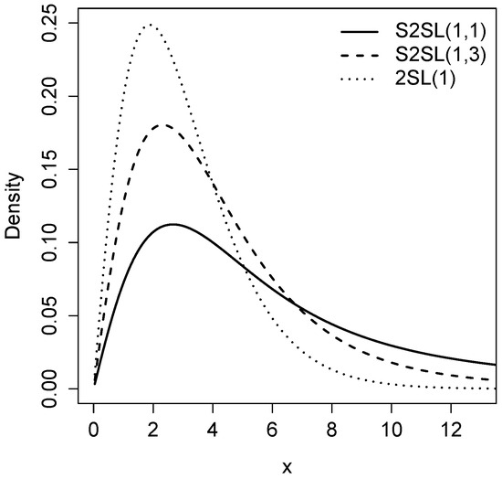
Figure 1. Graphical comparison of the pdf between the 2SL and S2SL distributions for a fixed beta ($\beta =1$) and different values of q.

2.2. Properties

Proposition 2. 

Let $X\sim S2LS(\beta ,q)$. Then the cumulative distribution function (cdf) of X is given by

$$F_X(x;\beta ,q)={\displaystyle \frac{{\left(\beta x\right)}^{-q}}{6{(1+\beta )}^2}}\{{\left(\beta x\right)}^q\left[{\gamma }_{4-q}+6\beta (\beta {\gamma }_{2-q}+{\gamma }_{3-q})\right]-6\beta (\beta {\gamma }_2+{\gamma }_3)-{\gamma }_4\}.$$

Proof. 

Using the definition of cdf and integrating by parts, the result is obtained.    □

Figure 2 presents a graphical comparison of the cdf of the S2SL model (with $\beta =1$) for different values of q, compared to the 2SL distribution.

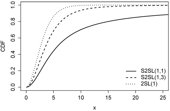
Figure 2. Graphical comparison of the cdf between the 2SL and S2SL distributions for a fixed beta ($\beta =1$) and different values of q.

The survival and hazard functions are defined as $R_X(x;\beta ,q)=1-F_X(x;\beta ,q)$ and $h_X(x;\beta ,q)=f_X(x;\beta ,q)/[1-F_X(x;\beta ,q)]$, respectively. These are two important functions in survival analysis because they represent the probability that an observation does not present the event of interest as a function of time, and the approximate probability of presenting the event of interest at the immediately following instant. For the S2SL distribution, these functions are presented in the following proposition.

Proposition 3. 

Let $X\sim S2SL(\beta ,q)$; then, the survival and hazard functions are given by

$$R_X(x;\beta ,q)={\displaystyle \frac{6{(1+\beta )}^2-{\left(\beta x\right)}^{-q}\{{\left(\beta x\right)}^q\left[{\gamma }_{4-q}+6\beta (\beta {\gamma }_{2-q}+{\gamma }_{3-q})\right]-6\beta (\beta {\gamma }_2+{\gamma }_3)-{\gamma }_4\}}{6{(1+\beta )}^2}},$$

$$h_X(x;\beta ,q)={\displaystyle \frac{q{x}^{-(q+1)}\{{\gamma }_4+6\beta \left[{\gamma }_3+\beta {\gamma }_2\right]\}}{6{\beta }^q{(1+\beta )}^2-x^{-q}\{{\left(\beta x\right)}^q\left[{\gamma }_{4-q}+6\beta (\beta {\gamma }_{2-q}+{\gamma }_{3-q})\right]-6\beta (\beta {\gamma }_2+{\gamma }_3)-{\gamma }_4\}}}.$$

Proof. 

Using the definitions of the survival and hazard functions,

$$R_X(x;\beta ,q)=1-F_X(x;\beta ,q);h_X(x;\beta ,q)={\displaystyle \frac{f_X(x;\beta ,q)}{1-F_X(x;\beta ,q)}},$$

and replacing $f_X(x;\beta ,q)$ and $F_X(x;\beta ,q)$, the result is obtained.    □

Figure 3, shows the survival function (left) and hazard function (right) $\beta =1$ and different values of q, compared with the 2SL distribution.

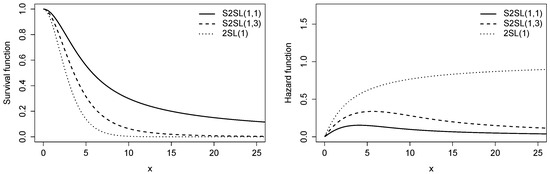
Figure 3. Plots of the survival function (left) and the hazard function (right) for the S2SL distribution with $\beta =1$ and different values of q, compared to the 2SL distribution.

Table 1 shows $P(X>x)$ for different values of x in the mentioned distribution.

Table 1. Comparison of the tails of the 2SL and S2SL distributions.

Distribution	$\mathit{P}(\mathit{X}>5)$	$\mathit{P}(\mathit{X}>10)$	$\mathit{P}(\mathit{X}>15)$
S2SL (1, 1)	0.5586	0.2995	0.2000
S2SL (1, 5)	0.2428	0.0267	0.0041
S2SL (1, 10)	0.1876	0.0104	0.0005
2SL (1)	0.1387	0.0041	0.0001

The size of the right tail of a distribution is crucial when the chosen model aims to capture values far from the beginning of the distribution’s support, such as outliers. The concept of heavy tails is fundamental in actuarial statistical applications. In this context, distributions such as Pareto, Lognormal, and Weibull, among others, have been widely used to model losses in automobile insurance and catastrophic insurance. It is well-established that any probability distribution defined by its cdf $F_X\left(x\right)$ on the real line is classified as heavy right-tailed (see Rolski et al. [23]) if $lim{sup}_{x\to \infty }(-log\left(R_X\left(x\right)\right)/x)=0$. An important topic in extreme value theory is regular variation (see Bingham [24]), a concept formalized in the following definition.

Definition 1. 

A distribution function is called regular varying at infinity with index $-\alpha$ si

$$\underset{x\to \infty }{lim}{\displaystyle \frac{R_X\left(tx\right)}{R_X\left(x\right)}}=t^{-\alpha },$$

(3)

where the parameter $\alpha \ge 0$ is called the tail index.

The following proposition states that the survival function of the S2SL distribution exhibits regular variation.

Proposition 4. 

The survival function of the random variable $X\sim S2SL(\beta ,q)$ is a survival function with regularly varying tails.

Proof. 

Applying the above definition and using L’Hospital’s rule we have that

$$\underset{x\to \infty }{lim}{\displaystyle \frac{R_X\left(tx\right)}{R_X\left(x\right)}}=t\underset{x\to \infty }{lim}{\displaystyle \frac{f_X(tx;\beta ,q)}{f_X(x;\beta ,q)}}=t^{-q}\underset{x\to \infty }{lim}{\displaystyle \frac{\gamma (q+4,\beta tx)+6\beta \left[\gamma (q+3,\beta tx)+\beta \gamma (q+2,\beta tx)\right]}{\gamma (q+4,\beta x)+6\beta \left[\gamma (q+3,\beta x)+\beta \gamma (q+2,\beta x)\right]}}.$$

Since ${lim}_{x\to \infty }\gamma (q+i,\beta tx)={lim}_{x\to \infty }\gamma (q+i,\beta x)=\Gamma (q+i)$, the result is obtained when calculating the limit.    □

A direct consequence of the above proposition is that the S2SL distribution is heavy right-tailed (see Rolski et al. [23]).

Proposition 5 shows that the S2SL distribution is the product of a scale mixture between the 2SL and Beta distributions.

Proposition 5. 

Let $X|W=w\sim 2SL\left(w^{-1},\beta \right)$ and $W\sim Beta(q,1)$. Then, $X\sim S2SL(\beta ,q)$.

Proof. 

The marginal density function of X is given by

$$\begin{array}{cc}\hfill f_X(x;\beta ,q)& ={\int }_0^1{f}_{X|W}\left(x\right|w)·f_W\left(w\right)dw,\hfill \\ \hfill & ={\int }_0^1{\displaystyle \frac{w^2{\beta }^4}{{(1+\beta )}^2}}x\left({\displaystyle \frac{w^2{x}^2}{6}}+wx+1\right)e^{-\beta xw}·q{w}^{q-1}dw,\hfill \\ \hfill & ={\displaystyle \frac{x{\beta }^{4}q}{{(1+\beta )}^2}}\left[{\displaystyle \frac{x^2}{6}}{\int }_0^1{w}^{q+3}{e}^{-\beta xw}dw+x{\int }_0^1{w}^{q+2}{e}^{-\beta xw}dw+{\int }_0^1{w}^{q+1}{e}^{-\beta xw}dw\right].\hfill \end{array}$$

Finally, substituting the variable $u=\beta xw$, the result is obtained.    □

Proposition 6. 

Let $X\sim S2SL(\beta ,q)$. If $q\to \infty$, then $X\stackrel{D}{\to }2SL\left(\beta \right)$, where $\stackrel{D}{\to }$ denotes convergence in the distribution.

Proof. 

Let $X\sim S2SL(\beta ,q)$ and $X={\displaystyle \frac{Y}{U^{1/q}}}$ given in (2). First, we study the convergence in the probability of $U^{1/q}$. We have that, $U\sim U(0,1)$ and $W=U^{1/q}\sim Beta(q,1)$. Thus, we obtain

$$E\left[{(W-1)}^2\right]={\displaystyle \frac{2}{{(q+1)}^2(q+2)}},$$

where if $q\to \infty \Rightarrow$$E\left[{(W-1)}^2\right]\to 0$. Therefore, $W\stackrel{P}{\to }1$, where $\stackrel{P}{\to }$ denotes convergence in probability. Finally, applying Slutsky’s theorem for $X={\displaystyle \frac{Y}{W}}$, we have that $X\stackrel{D}{\to }Y\sim 2SL\left(\beta \right)$.    □

2.3. Moments

Proposition 7. 

Let $X\sim S2SL(\beta ,q)$, then the r-th moment of X is given by

$${\mu }_r=E\left[X^r\right]={\displaystyle \frac{q(r+1)!}{6{\beta }^r(q-r){(1+\beta )}^2}}\left[6{\beta }^2+6\beta (r+2)+r^2+5r+6\right].$$

Proof. 

Using the stochastic representation given in (2), we have that

$$\begin{array}{cc}\hfill {\mu }_r& =E\left[X^r\right]=E\left[{\left({\displaystyle \frac{Y}{U^{\frac{1}{q}}}}\right)}^r\right]=E\left[Y^r\right]·E\left[U^{-{\displaystyle \frac{r}{q}}}\right],\hfill \end{array}$$

where $E[U^{-{\displaystyle \frac{r}{q}}}]={\displaystyle \frac{q}{q-r}}$, $q>r$ and $E\left[Y^r\right]={\displaystyle \frac{(r+1)!}{6{\beta }^r{(1+\beta )}^2}}\left[6{\beta }^2+6\beta (r+2)+r^2+5r+6\right]$, are the r-th moments of $U^{-{\displaystyle \frac{1}{q}}}$ and Y, respectively, where $U\sim U(0,1)$ and $Y\sim 2SL\left(\beta \right)$.    □

Corollary 1. 

If $X\sim S2SL(\beta ,q)$ with β and $q>0$, the first four moments and variance of X are

$${\mu }_1=E\left[X\right]={\displaystyle \frac{2q(\beta +2)}{\beta (q-1)(1+\beta )}},q>1.$$

$${\mu }_2=E\left[X^2\right]={\displaystyle \frac{2q(3{\beta }^2+12\beta +10)}{{\beta }^2(q-2){(1+\beta )}^2}},q>2.$$

$${\mu }_3=E\left[X^3\right]={\displaystyle \frac{24q({\beta }^2+5\beta +5)}{{\beta }^3(q-3){(1+\beta )}^2}},q>3.$$

$${\mu }_4=E\left[X^4\right]={\displaystyle \frac{120q({\beta }^2+6\beta +7)}{{\beta }^4(q-4){(1+\beta )}^2}},q>4.$$

$$V\left(X\right)={\displaystyle \frac{2q\left({\beta }^2{q}^2-2{\beta }^{2}q+3{\beta }^2+4\beta q^2-8\beta q+12\beta +2q^2-4q+10\right)}{b^2{(1+\beta )}^2(q-2){(q-1)}^2}},q>2.$$

The asymmetry and kurtosis coefficients are defined as $E\left(Z^3\right)$ and $E\left(Z^4\right)$, respectively, where $Z=(X-E\left(X\right))/\sqrt{\mathrm{Var}\left(X\right)}$ represents the standardized variable. These coefficients are of great importance, since the first allows us to quantify the degree of asymmetry of a variable, while the kurtosis coefficient can be used to detect the presence of heavy tails in the underlying distribution. The following proposition presents these coefficients for the S2SL distribution.

Proposition 8. 

Let $Y\sim S2SL(\beta ,q)$; then, the asymmetry and kurtosis coefficients of the random variable Y are given by

$$\sqrt{{\beta }_1}={\displaystyle \frac{24{\kappa }_3({\beta }^2+5\beta +5)-12{\kappa }_1{\kappa }_2({\beta }^2+3\beta +2)(3{\beta }^2+12\beta +10)+16{\kappa }_1^3{({\beta }^2+3\beta +2)}^3}{{\left[2{\kappa }_2(3{\beta }^2+12\beta +10)-4{\kappa }_1^2{({\beta }^2+3\beta +2)}^2\right]}^{3/2}}},$$

$${\beta }_2={\displaystyle \frac{120{\kappa }_4({\beta }^2+6\beta +7)-192{\kappa }_1{\kappa }_3({\beta }^2+3\beta +2)({\beta }^2+5\beta +5)+48{\kappa }_1^2{\kappa }_2{({\beta }^2+3\beta +2)}^2(3{\beta }^2+12\beta +10)-48{\kappa }_1^4{({\beta }^2+3\beta +2)}^4}{{\left(2{\kappa }_2(3{\beta }^2+12\beta +10)-4{\kappa }_1^2{({\beta }^2+3\beta +2)}^2\right)}^2}},$$

where ${\kappa }_r(\beta ,q)={\displaystyle \frac{q}{{\beta }^r(q-r){(1+\beta )}^2}}$.

Proof. 

Using the definitions of the standardized asymmetry and kurtosis coefficients,

$$\begin{array}{c}\hfill \sqrt{{\beta }_1}={\displaystyle \frac{E\left[{(X-E\left(X\right))}^3\right]}{{\left(V\left(X\right)\right)}^{3/2}}}={\displaystyle \frac{{\mu }_3-3{\mu }_1{\mu }_2+2{\mu }_1^3}{{\left({\mu }_2-{\mu }_1^2\right)}^{3/2}}},\mathrm{and}\\ \hfill {\beta }_2={\displaystyle \frac{E\left[{(X-E\left(X\right))}^4\right]}{{\left(V\left(X\right)\right)}^2}}={\displaystyle \frac{{\mu }_4-4{\mu }_1{\mu }_3+6{\mu }_1^2{\mu }_2-3{\mu }_1^4}{{\left({\mu }_2-{\mu }_1^2\right)}^2}},\end{array}$$

where ${\mu }_1$, ${\mu }_2$, ${\mu }_3$ and ${\mu }_4$ are given by Corollary 1. The result is obtained by substituting the corresponding terms.    □

Figure 4 shows that when the values of parameter q are low, the asymmetry and kurtosis coefficients increase.

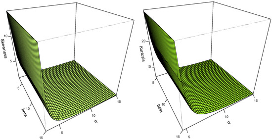
Figure 4. Graphs of the asymmetry and kurtosis coefficients of the S2SL ($\beta ,q$) model.

3. Inference

In this section, we carry out parameter estimation of the S2SL distribution using the moments and ML methods with the EM algorithm, and perform a simulation study.

3.1. Moments Estimators

Proposition 9. 

Let $X_1,X_2,\dots ,X_n$ be a random sample from $X\sim S2SL(\beta ,q)$, then the moments estimators of $\theta =(\beta ,q)$ are given by

$${\widehat{q}}_M={\displaystyle \frac{\overline{X}{\widehat{\beta }}_M(1+{\widehat{\beta }}_M)}{\overline{X}{\widehat{\beta }}_M(1+{\widehat{\beta }}_M)-2({\widehat{\beta }}_M+2)}},$$

(4)

$${\displaystyle \frac{\overline{X}(1+{\widehat{\beta }}_M)\left({\widehat{\beta }}_M^2{(1+{\widehat{\beta }}_M)}^2\overline{X^2}-2(3{\widehat{\beta }}_M^2+12{\widehat{\beta }}_M+10)\right)}{\overline{X}{\widehat{\beta }}_M(1+{\widehat{\beta }}_M)-2({\widehat{\beta }}_M+2)}}-2{\widehat{\beta }}_M^2{(1+{\widehat{\beta }}_M)}^2\overline{X^2}=0,$$

(5)

where $\overline{X}$ is the sample mean and $\overline{X^2}$ is the sample mean of the squares of sample units. We solve Equation (5) numerically to obtain ${\widehat{\beta }}_M$. Then, ${\widehat{\beta }}_M$ must be replaced in Equation (4) to obtain ${\widehat{q}}_M$.

Proof. 

Using Proposition 7 and substituting $E\left[X\right]$ by $\overline{X}$ and $E\left[X^2\right]$ by $\overline{X^2}$, the following equations are obtained:

$$\overline{X}={\displaystyle \frac{2q(\beta +2)}{\beta (q-1)(1+\beta )}},$$

(6)

$$\overline{X^2}={\displaystyle \frac{2q(3{\beta }^2+12\beta +10)}{{\beta }^2(q-2){(1+\beta )}^2}}.$$

(7)

Solving Equation (6) for parameter q, we obtain Equation (4). Then, replacing ${\widehat{q}}_M$ in Equation (7), we obtain Equation (5).    □

3.2. ML Estimators

Let $X_1,\dots ,X_n$, be a random sample of size n of a random variable X with $S2SL(\beta ,q)$ distribution, then the log-likelihood function for $\theta ={(\beta ,q)}^T$ can be expressed as

$$\begin{array}{ccc}\hfill \mathsf{\ell }(\theta ,x_i)& \propto & nlog\left(q\right)-(q+1)\sum _{i=1}^{n}log\left(x_i\right)-nqlog\left(\beta \right)-2nlog(1+\beta )\hfill \\ & +& \sum _{i=1}^{n}log\left[\gamma (q+4,\beta x_i)+6\beta \left[\gamma (q+3,\beta x_i)+\beta \gamma (q+2,\beta x_i)\right]\right].\hfill \end{array}$$

(8)

Deriving partially the log-likelihood function for $\beta$ and q and equalling to zero, we obtain the following equations:

$${\displaystyle {\displaystyle \frac{\partial \mathsf{\ell }(\theta ,x_i)}{\partial \beta }}=-\frac{nq}{\beta }-\frac{2n}{1+\beta }+\sum _{i=1}^n\frac{6\gamma (q+3,\beta x_i)+12\beta \gamma (q+2,\beta x_i)+{\beta }^{q+3}{x}_i^{q+2}{e}^{-\beta x_i}(x_i^2+6x_i+6)}{\gamma (q+4,\beta x_i)+6\beta \left[\gamma (q+3,\beta x_i)+\beta \gamma (q+2,\beta x_i)\right]}=0,}$$

(9)

$${\displaystyle \frac{\partial \mathsf{\ell }(\theta ,x_i)}{\partial q}}={\displaystyle \frac{n}{q}}-\sum _{i=1}^{n}log\left(x_i\right)-nlog\left(\beta \right)+\sum _{i=1}^n{\displaystyle \frac{\mathcal{I}(q+4,\beta x_i)+6\beta \left[\mathcal{I}(q+3,\beta x_i)+\beta \mathcal{I}(q+2,\beta x_i)\right]}{\gamma (q+4,\beta x_i)+6\beta \left[\gamma (q+3,\beta x_i)+\beta \gamma (q+2,\beta x_i)\right]}}=0,$$

(10)

where ${\displaystyle \mathcal{I}(a,v)={\int }_0^v{t}^{a-1}log\left(t\right)e^{-t}dt}$, $a>0$, and $v>0$ (see Milgram [25]) where $\mathcal{I}(a,v)$ is related with the generalized integral-exponential function when $v=\infty$.

The solutions to Equations (9) and (10) can be obtained using digital methods like the Newton–Raphson algorithm. One alternative for obtaining the ML estimators is to maximize Equation (8) using the optim function of the R software [26] version 4.0.5. However, in order to obtain a more robust estimation procedure, in the next subsection we will explore the use of the EM algorithm for this particular problem.

3.3. EM Algorithm

The EM algorithm (see Dempster et al. [27]) is a widely used tool for estimating ML in scenarios with unobserved or latent data. In this context, the S2SL distribution can also be expressed by the following stochastic approach.

$$\begin{array}{cc}\hfill Y_i\mid Z_{1i}=z_{1i},Z_{2i}=z_{2i},U_i=u_i& \sim G(2+z_{1i}+z_{2i},\beta y_i),\hfill \\ \hfill Z_{1i}& \sim \mathrm{Bern}\left({\displaystyle \frac{1}{1+\beta }}\right),\hfill \\ \hfill Z_{2i}& \sim \mathrm{Bern}\left({\displaystyle \frac{1}{1+\beta }}\right),\hfill \\ \hfill U_i& \sim \mathrm{Beta}(q,1).\hfill \end{array}$$

(11)

where $Z_{1i},Z_{2i}$ and $U_i$, for $i=1,\dots ,n$ represent the unobserved variables. The data observed are given by ${\mathbf{D}}_o={\mathbf{y}}^{\top }$, where ${\mathbf{y}}^{\top }=(y_i,\dots ,y_n)$. The vectors ${\mathbf{z}}_{\mathbf{1}}^{\top }=(z_{1i},\dots ,z_{1n})$, ${\mathbf{z}}_{\mathbf{2}}^{\top }=(z_{2i},\dots ,z_{2n})$ and ${\mathbf{u}}^{\top }=(u_i,\dots ,u_n)$ are the latent variables and the vector ${\mathbf{D}}_c={({\mathbf{y}}^{\top },{\mathbf{z}}_{\mathbf{1}}^{\top },{\mathbf{z}}_{\mathbf{2}}^{\top },{\mathbf{u}}^{\top })}^{\top }$ are the complete data. The joint distribution of $(Y_i,Z_{1i},Z_{2i},U_i)$ is given by

$$\begin{array}{cc}\hfill f(y_i,z_{1i},z_{2i},u_i)=& f(y_i\mid z_{1i},z_{2i},u_i)\times f\left(z_{1i}\right)\times f\left(z_{2i}\right)\times f\left(u_i\right),\hfill \\ \hfill =& {\displaystyle \frac{{\left(\beta u_i\right)}^{2+z_{1i}+z_{2i}}}{\Gamma (2+z_{1i}+z_{2i})}}{y}_i^{1+z_{1i}+z_{2i}}{e}^{-\beta u_i{y}_i}\times {\left({\displaystyle \frac{1}{1+\beta }}\right)}^{z_{1i}+z_{2i}}{\left({\displaystyle \frac{\beta }{1+\beta }}\right)}^{2-(z_{1i}+z_{2i})}\times q{u}_i^{q-1},\hfill \\ \hfill =& {\displaystyle \frac{q{\beta }^4{\left(u_i\right)}^{2+z_{1i}+z_{2i}+q-1}}{\Gamma (2+z_{1i}+z_{2i}){(1+\beta )}^2}}{y}_i^{1+z_{1i}+z_{2i}}{e}^{-\beta u_i{y}_i}.\hfill \end{array}$$

Thus the complete log-likelihood function for $\theta =(\beta ,q)$ can be expressed as

$${\mathsf{\ell }}_c(\theta ;D_c)=n[4log\beta -2log(1+\beta )+logq]-\beta \sum _{i=1}^n{u}_i{y}_i+q\sum _{i=1}^{n}log{u}_i+c,$$

where c is a constant that does not depend on the parameters vector. Thus the expected ${\mathsf{\ell }}_c(\theta ;D_c)$, given by the observed data, is

$$Q(\theta \mid {\theta }^{\left(k\right)})=n[4log\beta -2log(1+\beta )+logq]-\beta \sum _{i=1}^n{\widehat{u_i}}^{\left(k\right)}{y}_i+q\sum _{i=1}^n{\widehat{{\kappa }_i}}^{\left(k\right)},$$

where $\widehat{u_i}=\mathbb{E}(U_i\mid y_i)$ and $\widehat{k_i}=\mathbb{E}(log{U}_i\mid y_i)$. Note that

$$\begin{array}{cc}\hfill f(u_i,z_{1i},z_{2i}\mid y_i)& \propto \underset{\begin{array}{c}{U}_i\mid z_{1i},z_{2i},y_i\sim T{G}_{(0,1)}(2+z_{1i}+z_{2i}+q,\beta y_i)\end{array}}{\underbrace{{\displaystyle \frac{{\left(\beta y_i\right)}^{2+z_{1i}+z_{2i}+q}}{\Gamma (2+z_{1i}+z_{2i}+q)}}·{\displaystyle \frac{u_i^{(2+z_{1i}+z_{2i}+q)-1}{e}^{-\beta y_i{u}_i}}{G(1;2+z_{1i}+z_{2i}+q,\beta y_i)}}}}\hfill \\ \hfill & \times \underset{\begin{array}{c}{Z}_{1i},Z_{2i}\mid y_i\sim \mathrm{Bernoulli}\left(v_i\right)\end{array}}{\underbrace{{\displaystyle \frac{\Gamma (2+z_{1i}+z_{2i}+q)}{\Gamma (2+z_{1i}+z_{2i})}}{\beta }^{-z_{1i}-z_{2i}}G(1;2+z_{1i}+z_{2i}+q,\beta y_i)}}\hfill \end{array}$$

(12)

where $v_i={\displaystyle \frac{6\beta \Gamma (3+q)G_3+\Gamma (4+q)G_4}{6{\beta }^2\Gamma (2+q)G_2+6\beta \Gamma (3+q)G_3+\Gamma (4+q)G_4}}$, $G(y;a)={\int }_0^y{\displaystyle \frac{1}{\Gamma \left(a\right)}}{t}^{a-1}{e}^{-t}dt$ is the cdf of the gamma model. Furthermore, we define $G_p=G(\beta y_i;q+p)$ and $T{G}_{(0,1)}(a,b)$; this denotes the gamma distribution with shape parameter a and rate b truncated in the interval $(0,1)$.

Therefore, using properties of conditional expectations, we have that $\mathbb{E}(U_i\mid y_i)=\mathbb{E}[\mathbb{E}(U_i\mid Z_{1i},Z_{2i},y_i)\mid y_i]$; according to (12), this expectation is simple to compute, and we obtain $\mathbb{E}(log{U}_i\mid y_i)$ similarly. The results are as follows:

$$\mathbb{E}(U_i\mid y_i)={\displaystyle \frac{1}{\beta y_i\mathcal{S}}}\left[\Gamma (2+q)(2+q)G_3+{\displaystyle \frac{\Gamma (3+q)(3+q)G_4}{\beta }}+{\displaystyle \frac{\Gamma (4+q)(4+q)G_5}{6{\beta }^2}}\right],$$

(13)

$$\mathbb{E}(\log U_i\mid y_i)=-log\left(\beta y_i\right)+{\displaystyle \frac{\mathcal{I}(q+2,\beta y_i)}{\mathcal{S}}}+{\displaystyle \frac{\mathcal{I}(q+3,\beta y_i)}{\beta \mathcal{S}}}+{\displaystyle \frac{\mathcal{I}(q+4,\beta y_i)}{6{\beta }^2\mathcal{S}}},$$

(14)

where $\mathcal{S}$ is the normalization constant, defined as

$$\mathcal{S}=\Gamma (2+q)G_2+{\displaystyle \frac{\Gamma (3+q)G_3}{\beta }}+{\displaystyle \frac{\Gamma (4+q)G_4}{6{\beta }^2}}.$$

Thus, the EM algorithm for estimating the vector $\theta =(\beta ,q)$ is as follows:

• Step E: given ${\widehat{\beta }}^{(k-1)}$ and ${\widehat{q}}^{(k-1)}$, for $i=1,\dots ,n$ compute ${\widehat{u_i}}^{\left(k\right)}$ and ${\widehat{k_i}}^{\left(k\right)}$ using Equations (13) and (14).
• Step M1: update ${\widehat{q}}^{\left(k\right)}$ as,

  $${\widehat{q}}^{\left(k\right)}={\displaystyle \frac{-n}{{\sum }_{i=1}^n{\widehat{k_i}}^{\left(k\right)}}}.$$
• Step M2: update ${\widehat{\beta }}^{\left(k\right)}$ as the solution of the following non-linear equation

  $${\displaystyle \frac{4n}{\beta }}-{\displaystyle \frac{2n}{1+\beta }}=\sum _{i=1}^n{y}_i{\widehat{u_i}}^{\left(k\right)}.$$

Steps E, M1, and M2 are repeated until convergence is reached, defined when the difference between the estimations of two consecutive iterations is less than a previously fixed value. Note that Step M1 has an explicit solution, while $\beta$ can be solved using, for example, the uniroot function in R.

3.4. Simulation Study

In this section, we present a simulation study to evaluate the performance of the EM algorithm in estimating the parameters of the S2SL distribution. A total of 1000 replicas were generated for four sample sizes: $n=50,100,200$ and 500, using fixed values for parameters $\beta$ and q. The initial values to start the EM algorithm are ${\beta }^{\left(0\right)}=1$ and $q^{\left(0\right)}=1$. Based on the stochastic representation given in Equation (11), random numbers can be generated from the S2SL model, leading to Algorithm 1.

Algorithm 1 For simulating values from the distribution $X\sim S2SL(\beta ,q)$

1: Generate $Z_{1i}\sim \mathrm{Bernoulli}\left({\displaystyle \frac{1}{1+\beta }}\right),i=1,2,\dots ,n$. 2: Generate $Z_{2i}\sim \mathrm{Bernoulli}\left({\displaystyle \frac{1}{1+\beta }}\right),i=1,2,\dots ,n$. 3: Generate $U_i\sim \mathrm{Beta}(q,1),i=1,2,\dots ,n$. 4: Compute $X_i=\mathrm{Gamma}(2+Z_{1i}+Z_{2i},U_i\beta )\sim S2SL(\beta ,q),i=1,2,\dots ,n$.

Table 2 shows the estimated mean for each parameter (Mean), together with their standard errors (SE), the root mean squared error (RMSE), and the coverage percentage (CP) of the ML estimators, based on a 95% confidence interval. It may be concluded from the results that the ML estimators are consistent. As the sample size increases, the estimation means draw progressively closer to the true value of the parameter. As might be expected, the values of the SE and the RMSE diminish and stabilize as the sample size increases, suggesting that the standard errors of the estimators are calculated correctly. The R codes are available in Appendix A.

Table 2. Simulation study for the parameters of $\beta$ and q in the S2SL model.

True Value			$\mathit{n}=50$				$\mathit{n}=100$				$\mathit{n}=200$				$\mathit{n}=500$
$\mathit{\beta }$	$\mathit{q}$	Estim.	Mean	SE	RMSE	CP	Mean	SE	RMSE	CP	Mean	SE	RMSE	CP	Mean	SE	RMSE	CP
2	0.5	$\widehat{\beta }$	2.022	0.410	0.403	0.939	2.020	0.288	0.288	0.949	2.004	0.201	0.207	0.94	2.013	0.128	0.125	0.951
		$\widehat{q}$	0.515	0.091	0.099	0.949	0.505	0.063	0.065	0.955	0.503	0.044	0.046	0.94	0.497	0.027	0.027	0.948
	1	$\widehat{\beta }$	1.999	0.338	0.356	0.941	1.996	0.237	0.232	0.948	2.000	0.168	0.161	0.954	2.002	0.106	0.108	0.941
		$\widehat{q}$	1.080	0.246	0.297	0.970	1.030	0.159	0.167	0.970	1.014	0.109	0.114	0.961	1.004	0.068	0.068	0.954
	1.5	$\widehat{\beta }$	1.973	0.315	0.318	0.934	2.005	0.224	0.221	0.945	1.995	0.157	0.160	0.934	1.996	0.099	0.093	0.961
		$\widehat{q}$	1.765	0.680	1.969	0.960	1.577	0.302	0.324	0.967	1.546	0.204	0.220	0.954	1.521	0.124	0.126	0.958
4	0.5	$\widehat{\beta }$	4.019	0.873	0.898	0.918	4.034	0.618	0.622	0.940	4.046	0.438	0.448	0.945	4.014	0.274	0.275	0.949
		$\widehat{q}$	0.519	0.094	0.101	0.945	0.504	0.063	0.065	0.951	0.499	0.044	0.045	0.946	0.498	0.028	0.028	0.947
	1	$\widehat{\beta }$	3.958	0.725	0.758	0.916	3.997	0.514	0.501	0.953	4.026	0.366	0.379	0.939	4.008	0.230	0.224	0.960
		$\widehat{q}$	1.103	0.270	0.375	0.968	1.043	0.165	0.180	0.961	1.012	0.111	0.119	0.937	1.004	0.069	0.068	0.953
	1.5	$\widehat{\beta }$	3.966	0.691	0.714	0.932	4.019	0.487	0.506	0.929	4.000	0.341	0.349	0.937	3.996	0.215	0.222	0.936
		$\widehat{q}$	1.948	1.009	4.297	0.962	1.583	0.318	0.361	0.963	1.546	0.210	0.218	0.959	1.515	0.128	0.137	0.945
6	0.5	$\widehat{\beta }$	6.078	1.375	1.410	0.921	6.054	0.965	1.008	0.938	6.015	0.676	0.695	0.941	6.002	0.425	0.426	0.955
		$\widehat{q}$	0.522	0.094	0.106	0.946	0.509	0.065	0.068	0.953	0.505	0.045	0.048	0.948	0.503	0.028	0.028	0.943
	1	$\widehat{\beta }$	6.045	1.155	1.197	0.926	6.019	0.810	0.862	0.928	6.005	0.569	0.59	0.944	6.004	0.358	0.364	0.945
		$\widehat{q}$	1.075	0.253	0.294	0.953	1.035	0.166	0.180	0.963	1.016	0.113	0.12	0.949	1.008	0.070	0.069	0.953
	1.5	$\widehat{\beta }$	5.958	1.082	1.123	0.925	5.962	0.755	0.787	0.930	5.997	0.534	0.547	0.948	5.988	0.336	0.346	0.939
		$\widehat{q}$	1.931	1.136	4.178	0.964	1.623	0.340	0.414	0.957	1.544	0.213	0.220	0.967	1.525	0.130	0.140	0.942

4. Applications

In this section, we analyse two real datasets to evaluate the performance of the S2SL distribution in modelling data with high kurtosis. A comparison is made between the S2SL, 2SL, and LSD distributions, using the Akaike information criterion (AIC) presented in Akaike [28], and the Bayesian information criterion (BIC) proposed in Schwarz [29]. Below, we present the pdf of the LSD distribution (see Gui [17]):

$$f_Y(y;\theta ,\sigma ,q)={\displaystyle \frac{q{\theta }^2}{\sigma (1+\theta )}}{\int }_0^1\left(1+{\displaystyle \frac{yt}{\sigma }}\right)e^{-{\displaystyle \frac{\theta yt}{\sigma }}}{t}^{q}dt,y,\theta ,\sigma ,q>0.$$

4.1. Application 1: Patients with Acute Bone Cancer

The dataset contains the survival times (in days) of 73 patients diagnosed with acute bone cancer. The data were originally presented by Mansour et al. [30] and subsequently analysed by Klakattawi [31] and Alanzi et al. [32]. The dataset is available in the R software package [26] “ComRiskModel” with the “data_acutebcancer” database.

Table 3 presents the descriptive statistics of the data: sample mean, standard deviation, sample asymmetry and kurtosis coefficients. Figure 5 shows a boxplot for the patients with acute bone cancer dataset, which is seen to present atypical observations and high kurtosis ($b_2=51.78$).

Table 3. Descriptive statistics for the application to bone cancer patients.

n	$\overline{\mathit{x}}$	s	$\sqrt{{\mathit{b}}_1}$	${\mathit{b}}_2$
73	3.76	10.60	6.80	51.78

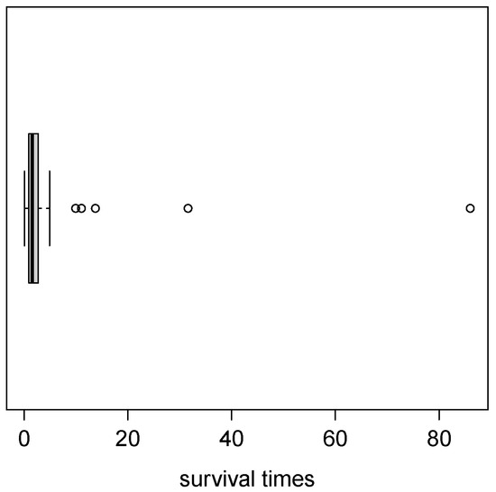
Figure 5. Boxplot for the bone cancer dataset.

The moments estimators for the parameters of the S2SL model are ${\widehat{\beta }}_M=1.4399$ and ${\widehat{q}}_M=1.0715$. These estimators were used as initial values to calculate the ML estimators. Table 4 shows the ML estimations with their standard errors and the AIC and BIC criteria. The S2SL distribution shows a better fit to the bone cancer patients dataset than the 2SL and LSD distributions, as the AIC and BIC values are smaller.

Table 4. Estimations for the 2SL, LSD and S2SL distributions.

Estimations	2SL (SE)	LSD (SE)	S2SL (SE)
$\widehat{\beta }$	0.8245 (0.0509)	-	2.4243 (0.2969)
$\widehat{\theta }$	-	0.0343 (0.0371)	-
$\widehat{\sigma }$	-	0.0233 (0.0258)	-
$\widehat{q}$	-	2.3092 (0.7187)	1.4611 (0.2903)
AIC	468.1453	290.0614	282.5487
BIC	470.4357	296.9328	287.1296

Figure 6 shows that the theoretical quantiles of the proposed S2SL model present a more exact fit to the quantiles of the survival data in the sample, when compared with the 2SL and LSD distributions. This supports the above finding, since according to the AIC and BIC selection criteria, the S2SL model presents a better fit to these dataset.

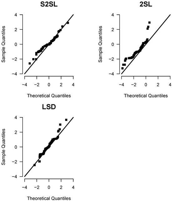
Figure 6. QQ-plot for the S2SL, 2SL, and LSD distributions for the bone cancer patients dataset.

4.2. Application 2: Air Transceiver Repair Times

The second application is to a set of 46 repair times for an air communications transceiver, measured in hours. The complete dataset was taken from Jorgensen [33]. Table 5 shows the descriptive statistics for the repair times, which present high kurtosis. Figure 7 shows the boxplot of the dataset, in which the existence of outliers can also be appreciated.

Table 5. Descriptive statistics for the application to repair times.

n	$\overline{\mathit{x}}$	s	$\sqrt{{\mathit{b}}_1}$	${\mathit{b}}_2$
40	4.01	5.17	1.85	10.02

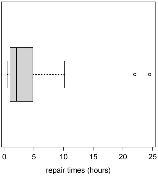
Figure 7. Boxplot for repair times dataset.

The moments estimators used as starting points for estimation by ML of the S2SL distribution are ${\widehat{\beta }}_M=1.2196$ and ${\widehat{q}}_M=1.0421$. Table 6 shows the ML estimates for the parameters, with their respective SE, and the values of the AIC and BIC criteria for each distribution compared. Figure 8 presents the QQ-plots for the 2SL, LSD and S2SL distributions. All these summaries and graphs enable us to conclude that the S2SL distribution provides the best fit to the repair times data.

Table 6. ML estimates for the 2SL, LSD and S2SL distributions.

Estimations	2SL (SE)	LSD (SE)	S2SL (SE)
$\widehat{\beta }$	0.7787 (0.0647)	-	2.0323 (0.4068)
$\widehat{\theta }$	-	0.0158 (0.0141)	-
$\widehat{\sigma }$	-	0.0113 (0.0102)	-
$\widehat{q}$	-	1.3333 (0.4079)	1.2423 (0.3462)
AIC	223.5754	189.9217	187.8777
BIC	225.2642	194.9884	191.2554

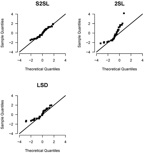
Figure 8. QQ-plot for the S2SL, 2SL and LSD distributions for the repair times data.

5. Conclusions

In this work, we present the S2SL distribution, an extension of the 2SL distribution in which the slash methodology is used to increase its flexibility for modelling data with heavy tails and outlying observations. Some properties of this new distribution are obtained, and its parameters are estimated by the ML method using the EM algorithm. Below, we highlight some of the most important characteristics of the S2SL distribution:

• The S2SL distribution has two different stochastic representations, given in Equation (2) and Proposition 5.
• The expressions of the pdf, cdf, and hazard function are obtained, all of which have a closed form and are represented by the lower incomplete gamma function.
• When the coefficients of asymmetry and kurtosis are analysed, the S2SL model is shown to be more flexible than the 2SL model. Furthermore, as shown in Table 1, the distribution tails become heavier as parameter q diminishes.
• Implementation of the EM algorithm allows ML estimators for the model parameters to be obtained more efficiently.
• The simulation study shows that as the sample size is increased, the ML estimators draw progressively closer to the true values of the parameters, suggesting that the estimators are consistent and stable.
• In the applications to real data, the S2LS distribution is seen to provide a better fit to the data when compared with the 2SL and LSD distributions, reflected in lower values in the AIC and BIC criteria.

In future work, we will consider exploring Bayesian inference for model parameters using the Bayesian bootstrap algorithm described by Lyddon et al. [34], as it represents a relevant complementary approach to the methodology presented in this study.

References

- Jonhson, N.L.; Kotz, S.; Balakrishnan, N. Continuous Univariate Distributions, 2nd ed.; Wiley: New York, NY, USA, 1995; Volume 1. [Google Scholar]
- Rogers, W.H.; Tukey, J.W. Understanding some long-tailed symmetrical distributions. Stat. Neerl. 1972, 26, 211–226. [Google Scholar] [CrossRef]
- Mosteller, F.; Tukey, J.W. Data Analysis and Regression; Addison-Wesley: Reading, MA, USA, 1977. [Google Scholar]
- Kafadar, K. A biweight approach to the one-sample problem. J. Am. Statist. Assoc. 1982, 77, 416–424. [Google Scholar] [CrossRef]
- Wang, J.; Genton, M.G. The multivariate skew-slash distribution. J. Stat. Plan. Inference 2006, 136, 209–220. [Google Scholar] [CrossRef]
- Gómez, H.W.; Quintana, F.A.; Torres, F.J. A New Family of Slash-Distributions with Elliptical Contours. Stat. Probab. Lett. 2007, 77, 717–725, Erratum in Erratum in Stat. Probab. Lett. 2008, 78, 2273–2274. [Google Scholar] [CrossRef]
- Olmos, N.M.; Varela, H.; Gómez, H.W.; Bolfarine, H. An extension of the half-normal distribution. Stat. Pap. 2012, 53, 875–886. [Google Scholar] [CrossRef]
- Olmos, N.M.; Varela, H.; Bolfarine, H.; Gómez, H.W. An extension of the generalized half-normal distribution. Stat. Pap. 2014, 55, 967–981. [Google Scholar] [CrossRef]
- Astorga, J.M.; Reyes, J.; Santoro, K.I.; Venegas, O.; Gómez, H.W. A Reliability Model Based on the Incomplete Generalized Integro-Exponential Function. Mathematics 2020, 8, 1537. [Google Scholar] [CrossRef]
- Rivera, P.A.; Barranco-Chamorro, I.; Gallardo, D.I.; Gómez, H.W. Scale Mixture of Rayleigh Distribution. Mathematics 2020, 8, 1842. [Google Scholar] [CrossRef]
- Lindley, D.V. Fiducial distributions and Bayes’ theorem. J. R. Stat. Soc. Ser. B 1958, 20, 102–107. [Google Scholar] [CrossRef]
- Ghitany, M.E.; Atieh, B.; Nadarajah, S. Lindley distribution and its applications. Math. Comput. Simul. 2008, 78, 493–506. [Google Scholar] [CrossRef]
- Ghitany, M.; Al-Mutairi, D.; Balakrishnan, N.; Al-Enezi, I. Power Lindley distribution and associated inference. Comput. Stat. Data Anal. 2013, 64, 20–33. [Google Scholar] [CrossRef]
- Gómez-Déniz, E.; Calderin-Ojeda, E. The discrete Lindley distribution: Properties and application. J. Stat. Comput. Simul. 2011, 81, 1405–1416. [Google Scholar] [CrossRef]
- Krishna, H.; Kumar, K. Reliability estimation in Lindley distribution with progressively type II right censored sample. Math. Comput. Simul. 2011, 82, 281–294. [Google Scholar] [CrossRef]
- Bakouch, H.S.; Al-Zaharani, B.; Al-Shomrani, A.; Marchi, V.; Louzada, F. An extended Lindley distribution. J. Korean Stat. Soc. 2012, 41, 75–85. [Google Scholar] [CrossRef]
- Gui, W. Statistical properties and applications of the Lindley slash distribution. J. Appl. Statist. Sci. 2012, 20, 283–298. [Google Scholar]
- Oluyede, B.O.; Yang, T. A new class of generalized Lindley distribution with applications. J. Stat. Comput. Simul. 2014, 85, 2072–2100. [Google Scholar] [CrossRef]
- Shanker, R.; Hagos, F.; Sujatha, S. On modeling of Lifetimes data using exponential and Lindley distributions. Biom. Biostat. Int. J. 2015, 2, 140–147. [Google Scholar] [CrossRef]
- Abouammoh, A.M.; Alshangiti, A.M.; Ragab, I.E. A new generalized Lindley distribution. J. Stat. Comput. Simul. 2015, 85, 3662–3678. [Google Scholar] [CrossRef]
- Tomy, L. A retrospective study on Lindley distribution. Biom. Biostat. Int. J. 2018, 7, 163–169. [Google Scholar] [CrossRef][Green Version]
- Chesneau, C.; Tomy, L.; Gillariose, J. On a Sum and Difference of two Lindley Distributions: Theory and Applications. REVSTAT 2020, 18, 673–695. [Google Scholar]
- Rolski, T.; Schmidli, H.; Schmidt, V.; Teugel, J. Stochastic Processes for Insurance and Finance; John Wiley & Sons: Hoboken, NJ, USA, 1999. [Google Scholar]
- Bingham, N. Regular Variation; Cambridge University Press: Cambridge, UK, 1987. [Google Scholar]
- Milgram, M.S. The generalized integro-exponential function. Math. Comput. 1985, 44, 443–458. [Google Scholar] [CrossRef]
- R Core Team. R: A Language and Environment for Statistical Computing; R Foundation for Statistical Computing: Vienna, Austria, 2023; Available online: https://www.r-project.org/ (accessed on 16 October 2024).
- Dempster, A.P.; Laird, N.M.; Rubim, D.B. Maximum likelihood from incomplete data via the EM algorithm (with discussion). J. R. Stat. Soc. Ser. B 1977, 39, 1–38. [Google Scholar] [CrossRef]
- Akaike, H. A new look at the statistical model identification. IEEE Trans. Automat. Contr. 1974, 19, 716–723. [Google Scholar] [CrossRef]
- Schwarz, G. Estimating the dimension of a model. Ann. Stat. 1978, 6, 461–464. [Google Scholar] [CrossRef]
- Mansour, M.; Yousof, H.M.; Shehata, W.A.; Ibrahim, M. A new two parameters Burr XII distribution: Properties, copula, different estimation methods and modeling acute bone cancer data. J. Nonlinear Sci. Appl. 2020, 13, 223–238. [Google Scholar] [CrossRef]
- Klakattawi, H.S. Survival analysis of cancer patients using a new extended Weibull distribution. PLoS ONE 2022, 17, e0264229. [Google Scholar] [CrossRef]
- Alanzi, A.R.; Imran, M.; Tahir, M.H.; Chesneau, C.; Jamal, F.; Shakoor, S.; Sami, W. Simulation analysis, properties and applications on a new Burr XII model based on the Bell-X functionalities. AIMS Math. 2023, 8, 6970–7004. [Google Scholar] [CrossRef]
- Jorgensen, B. Statistical Properties of the Generalized Inverse Gaussian Distribution; Lecture Notes in Statistics; Springer: New York, NY, USA, 1982. [Google Scholar]
- Lyddon, S.P.; Holmes, C.C.; Walker, S.G. General bayesian updating and the loss-likelihood bootstrap. Biometrika 2019, 106, 465–478. [Google Scholar] [CrossRef]
Disclaimer/Publisher’s Note: The statements, opinions and data contained in all publications are solely those of the individual author(s) and contributor(s) and not of MDPI and/or the editor(s). MDPI and/or the editor(s) disclaim responsibility for any injury to people or property resulting from any ideas, methods, instructions or products referred to in the content. |
© 2025 by the authors. Licensee MDPI, Basel, Switzerland. This article is an open access article distributed under the terms and conditions of the Creative Commons Attribution (CC BY) license (https://creativecommons.org/licenses/by/4.0/).