Utilizing Multifractal and Compositional Data Analysis Combined with Random Forest for Mineral Prediction in Goulmima, Morocco

Abstract

Morocco is rich in Mississippi Valley Type (MVT) copper deposits. Currently, geochemical surveying is being conducted in the Goulmima region in pursuit of breakthroughs in mineral exploration. This paper focuses on the delineation of prospecting targets in the Goulmima area based on the ongoing 1:100,000 geochemical survey work in Morocco. The study employs compositional data transformation to perform isometric log-ratio (ilr) transformations on raw data, followed by the Spectrum-Area (S-A) fractal processing, and then uses the Random Forest (RF) algorithm for mineral prediction. Finally, the prediction results are further delineated using the Concentration-Area (C-A) fractal model to identify high-probability areas, marking two prospecting targets. The results show: (1) the ilr transformation reduces the closure problem of the original data and improves their symmetry, thereby more effectively revealing the spatial structural features of the elements; (2) the principal component analysis (PCA) performed on the ilr-transformed data successfully identifies two main element combinations, representing high-temperature hydrothermal environments (Mo-Sn-Ti-W-U) and low-temperature mineralization environments (CaO-Pb-Zn), consistent with the regional mining history; (3) the application of the S-A multifractal model effectively distinguishes between anomalies and background distributions in the geochemical data of the study area, and combines fault buffer zones as the basis for mineral prediction; (4) the C-A fractal model further subdivides the prediction results, dividing potential mining areas into high, medium, and low probability zones, and ultimately identifies two prospecting targets.

1. Introduction

Mineral resource prediction is a crucial part of mineral exploration, aiming to delineate and screen prospective areas for undiscovered mineral resources in the study area based on studies of typical deposits. This involves analyzing and integrating various types of information including geology, mineral resources, geophysics, geochemistry, and remote sensing, further guiding mineral exploration efforts [1,2].

For regional mineral exploration, geochemical exploration is a direct and effective method [3,4,5]. For instance, in China, from 1981 to 2005, under the “National Geochemical Exploration Sweep Plan”, a total of 58,788 anomalies were delineated nationwide by the former Ministry of Geology and Mineral Resources and the Ministry of Land and Resources, leading to the discovery of 3349 mineral deposits, significantly contributing to the discovery of China’s mineral resources [6]. The processing methods for exploration geochemistry have also evolved rapidly over the decades, from initial single-element analysis (focused on locating a specific type of mineral in a particular area), to later multivariate analysis (as the interrelationships among geochemical elements became recognized), followed by subsequent non-linear analysis (recognizing the superimposed effects of geological actions on element enrichment), and to the current application of machine learning for deep data mining (enabled by the rapid development of computer technology, supporting more detailed data mining). After in-depth data mining, using these evidence layers along with mathematical prediction models, can better guide the direction for mineral prediction [7,8,9,10].

Commonly used mathematical models for mineral prediction include the weights of evidence model and its extended models [11,12], logistic regression [13], analytic hierarchy process, artificial neural networks [14,15], support vector machines [7], and extreme learning machines [16]. Additionally, given the powerful feature representation capabilities of machine learning/deep learning technologies, many scholars have recently attempted to introduce them into the field of geochemical anomaly identification and mineral prediction [8,17].

Random Forest (RF), with its advantages of being insensitive to multicollinearity, capable of handling high-dimensional data, tolerant to outliers and noise, unlikely to overfit, and high predictive accuracy, is one of the widely used ensemble algorithms across various fields [18,19]. Many scholars have also explored the application of Random Forest in the field of mineral prediction, demonstrating its superior accuracy and predictive performance [20,21,22,23], and noted that the Random Forest model also performs well with missing values and small training sample sets (fewer than 20 samples). Hariharan [24] applied the Random Forest algorithm for predicting the mineral prospectivity of gold deposits in the Tanami region in Western Australia, using synthetic minority oversampling techniques to modify the initial dataset and balance the ratio of deposits to non-deposits to approximately 50:50. They then objectively delineated the prospectivity areas through data sensitivity, specificity, and correct classification statistics. Carranza [25] utilized RF to build a prediction model for porphyry copper deposits in Catanduanes Island, Philippines, noting RF’s feasibility in data-driven modeling for areas with few mineral occurrences and handling predictive variables with missing values. Rodriguez Galiano [20] evaluated the performance of RF in predicting gold prospectivity in the Rodalquilar area in southern Spain, highlighting the advantages of using RF, including simple parameter settings, internal unbiased estimates of prediction error, the ability to handle complex data with different statistical distributions, the capability to model non-linear relationships between response variables, the use of categorical predictive variables, and the determination of variable importance.

This paper is based on the geochemical survey project conducted in collaboration between China and Morocco, aiming to better utilize geochemical exploration data for mineral prediction, further narrow down target areas, and provide key regions for subsequent exploration work. By applying composition data transformation and multivariate fractal modeling methods, appropriate individual elements and element combinations were selected. Combined with fault buffer zone distances, a mineral resource prediction model based on the Random Forest (RF) algorithm was constructed, successfully delineating favorable exploration areas.

2. Geological Background

2.1. Regional Geological Conditions

The Pre-Saharan Trough is located in southeastern Morocco, extending into the Souss-Massa-Drâa and Meknes-Tafilalet provinces. It forms a low-lying plain situated between the High Atlas Mountains to the north and the Anti-Atlas Mountains to the south (Figure 1). From west to east, the Pre-Saharan Trough can be subdivided into the Souss, Ouarzazate, and Errachidia-Boudnib-Erfoud basins [26]. The South Atlas fault delineates the Jurassic basins of the High Atlas to the north of the trough, flanked by the Precambrian and Palaeozoic formations of the Anti-Atlas to the south and the Tertiary formations of the Hamada du Guir to the east (see Figure 1). Overlying this, the Cretaceous strata of the Preafrican Trough rest unconformably on a basement consisting of either Palaeozoic or Jurassic rocks [27].

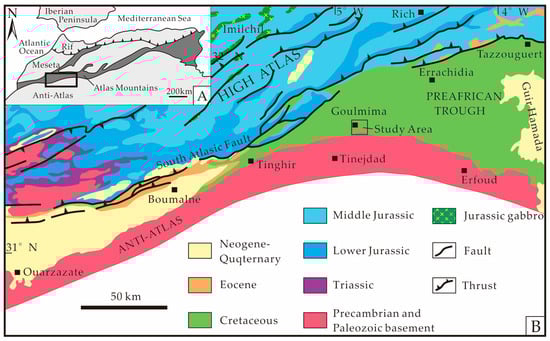
Figure 1. Tectonic location map of the study area (A. Tectonic setting; B. Regional geological map) [27].

2.2. Geological Features of Study Area

The Goulmima area exposes rocks from the Neoproterozoic Ediacaran, Paleozoic (including Cambrian, Ordovician, and Devonian periods), Mesozoic (including Triassic, Jurassic, and Cretaceous periods), and Quaternary periods (Figure 2).

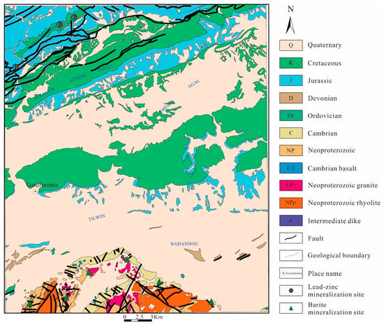
Figure 2. Geological map of the study area.

The Neoproterozoic Ediacaran period (NP3) in the Goulmima section is represented by weakly metamorphosed volcanic and clastic rock assemblies, regionally known as the Ouarzazate Group, which is unconformably overlain by Cambrian sandstones. Through regional comparisons, the Ediacaran strata in the Goulmima area are subdivided from bottom to top into volcanic rocks, volcaniclastic rock assemblies, and very shallowly metamorphosed clastic rock assemblies, primarily distributed in the southern part of the map area. The Cambrian (Є) primarily outcrops in the southeastern part of the Goulmima map, with conformable contact above with the Ordovician. The Ordovician (or) mainly outcrops in the southeastern corner of the map, in conformable contact below with the Cambrian. It is composed of grey-black silty mudstones, muddy siltstones, and white quartz sandstones, and can be subdivided from bottom to top into three lithological groups: or4, or5, and or6. The Devonian has limited exposure in Goulmima, mainly distributed in strips in the eastern part of the map, with the upper part overlain by Quaternary. The Triassic (t) has limited exposure in the Goulmima map, unconformably overlain by the Jurassic. The Jurassic primarily appears as a facies in the northern part of the map area, with the upper part consisting of a suite of brick-red claystone interbedded with salt rocks, and the lower part a suite of grey to green-grey clastic rocks and carbonate layers. The Cretaceous primarily outcrops in the northern part of the map area, mainly consisting of a suite of dolomitic carbonate rocks and clastic rock assemblies, overlain by Quaternary and in parallel unconformable contact with the underlying Jurassic.

The Goulmima area is characterized by active tectonic activities, with prominent effects from the Pan-African, Caledonian, Hercynian, and Alpine orogenies. The Neoproterozoic and early Paleozoic strata have undergone strong folding deformations, while the Mesozoic strata formed monoclinal structures under the influence of Alpine tectonic activities. The area also exhibits strong fault activity, predominantly NE-oriented normal faults, with a major NE-oriented reverse fault developed in the northern part of the study area (the South Atlas Fault (SAF)), and a series of NE-oriented faults exposed in the southern part. The Goulmima map is dominated by NE-oriented faults and NW-oriented faults (or NEE-oriented) faults. NE-oriented faults are mainly developed in the Triassic and Jurassic strata in the north side of the map and in the Neoproterozoic and early Paleozoic strata in the south side, where the NE (or NEE) faults in the northwest part control the lead-zinc mining and structural hydrothermal activities related to the minerals. Field geological characteristics show that this series of faults cuts through the Triassic and even Cretaceous strata, indicating that the formation of the faults is related to the late Alpine tectonic activities, and further fault activity becomes less recognizable due to the modification and destruction by later tectonic activities. In the south side of the map, NE-oriented faults developed in the Neoproterozoic Ediacaran, Cambrian, and Ordovician strata are generally smaller in scale compared to the northern faults, mostly associated with axial NE folds, often manifesting as near-NW compression, forming secondary faults on the wings of the folds. This group of faults controls the output of barite and fluorite minerals in the south side of the map. Major faults within the map area include the Tizi ’n first fault and the South Atlas fault, etc.

The Goulmima study area is located at the transition between the High Atlas and Middle Atlas Mountains, and overall, magmatic activity in the region is inactive. The exposed magmatic rocks are mainly basalts, granophyres, and some basic dykes. Magmatic activities can be divided into two phases: the first phase is related to the rifting of the Rheic Ocean during the early Paleozoic, involving basalts and intermediate-basic dykes mainly distributed in the southern part of the map in the Neoproterozoic and early Paleozoic Cambrian strata, controlled by NE-oriented faults. The second phase is related to the rifting of the North Atlantic during the late Triassic-early Jurassic, involving basalts and granophyres, mainly distributed in the cores of anticlines and near faults, regionally discontinuous.

2.3. Regional Mineral Characteristics

The study area has been influenced by multiple tectonic and magmatic activities during the Hercynian and Alpine orogenies, resulting in favorable conditions for mineralization in the region.

The primary types of mineral deposits in the study area include lead-zinc, barite, and fluorite, with genesis types encompassing MVT lead-zinc and hydrothermal vein barite and fluorite deposits. Among these, MVT lead-zinc (barite) deposits are the most prominent, characterized by vein and breccia bodies controlled by faults or fractures. Most ore bodies are affected by regional uplift, resulting in extensive secondary oxidation zones at the surface. The mineral assemblage mainly consists of galena (locally visible cerussite), sphalerite, smithsonite, iron-manganese oxides, and minor barite, with calcite as the primary gangue mineral. Hydrothermal vein barite deposits are predominantly found in the southern Little Atlas Mountains, controlled by NWW-oriented thrust faults and occurring along fractures. These deposits are widely distributed but generally small in scale, primarily mined by open pit methods.

3. Methods

3.1. Compositional Data Analysis

Conventional geochemical data, being compositional data, typically exhibit a “closure effect [28,29,30]”. The geometric space of this type of data belongs to Aitchison’s geometry, and its sample space is a simplex. The characteristic of compositional data lies in the fact that the sum of all components is fixed (the constant sum problem), and each component’s data is relative to the whole, which means it cannot fully capture the information in the entire dataset. In fact, geochemical data, as compositional data, typically exist in a non-closed form, meaning the sum is not fixed. Therefore, before applying compositional data transformations, we need to first “close” the data to ensure that the sum of each sample point equals 1 (100%). Vera Pawlowsky-Glahn [31] provided the latest definition of compositional data in 2015: “Compositional data are vector data composed of positive components that carry relative information.” In general, when there is a constant sum problem, any change in one component will induce changes in other components, indirectly causing the data of each part to be interrelated with the whole [32,33]. These characteristics lead to the closure effect in compositional data.

To quickly and effectively understand the structure and distribution of geochemical data, statistical methods are essential. However, most statistical methods are based on the premise that the data belong to Euclidean space, which includes statistical methods based on covariance and correlation matrices between variables, such as factor analysis, principal component analysis, cluster analysis, and discriminant analysis. If compositional data are not properly transformed when using these methods, the results may be flawed or even erroneous [34,35]. A particularly notable issue was raised by Piepel [33] in 1988 regarding the spurious correlation between variables. Since compositional data cannot independently vary as unconstrained data can, there is an implicit condition that at least one covariance (and thus correlation coefficient) must be negative. In this case, no correlation coefficient can freely vary between −1 and +1. Because the data are closed, spurious correlations arise between the components, typically leaning toward negative correlations. For instance, when only two variables are involved, and both exhibit a closure effect, their correlation must be −1. Additionally, when processing geochemical data, particularly when applying statistical methods to elements of interest or when adding new elements for subsequent statistical analysis, the introduction or removal of new variables (elements) will affect the other components in the overall dataset. Such changes may lead to a reversal of correlations between elements (positive to negative), thus resulting in spurious correlations between variables. Therefore transformed data generally offer more interpretable results when classical statistical methods are applied to untransformed data [3,34,36].

In compositional data analysis, the additive log-ratio transformation (alr), centered log-ratio transformation (clr), and isometric log-ratio transformation (ilr) are three commonly used transformations, each with its advantages and disadvantages. Essentially, both alr and clr transformations do not eliminate the closure effect of compositional data, whereas the ilr transformation does; after alr and ilr transformations, one variable is reduced; the data after clr transformation remains the same in terms of the number of variables, but the sum is “0” [36].

Considering the advantages and disadvantages of these three transformations, Filzmoser [34] suggested using the ilr transformation first to break the “closure effect” of the data, and then express the loadings of the ilr transformation in the clr space using a standard orthogonal basis. This approach not only overcomes the “closure effect” of geochemical data but also ensures the consistency of the number of variables before and after transformation, thereby facilitating more rational interpretations by geochemists [35]. Additionally, Filzmoser [34] also introduced the Robust Principal Component Analysis (RPCA) method to handle outliers in the data, which can effectively avoid poor covariance matrix estimates due to outliers when using PCA. Below are the theoretical formulas for each transformation:

Considering an original data matrix X_ij (m × n, where m is the number of samples and n is the number of elements), two transformations are introduced.

(1)

clr transformation:

$$clr\left(X_j\right)=\ln \left[{\displaystyle \frac{x_{1j}}{g\left(x_1\right)}},{\displaystyle \frac{x_{2j}}{g\left(x_2\right)}},\cdots \hspace{0.17em},{\displaystyle \frac{x_{mj}}{g\left(x_m\right)}}\right]$$

(1)

x is the elemental content at that point; j = 1, 2, …, n; g(x_i) is the geometric mean value of the “i”-th sample.

(2)

ilr transformation:

The ilr transformation is derived based on the clr transformation and the standard orthonormal basis vectors “v_j” [34].

$${\nu }_j=\sqrt{{\displaystyle \frac{j}{j+1}}}\left[{\displaystyle \frac{1}{j}},\cdots \hspace{0.17em},{\displaystyle \frac{1}{j}},-1,0,\cdots ,0\right]$$

(2)

$$ilr\left(X_j\right)=\sqrt{{\displaystyle \frac{j}{j+1}}}\ln {\displaystyle \frac{\sqrt[j]{{\prod }_{k=1}^j{x}_k}}{x_{j+1}}}, j=1, 2, \dots , n-1$$

(3)

3.2. Multifractal Analysis

Changes in geological historical periods affect the spatial distribution of geochemical element contents [3,37,38]. The complex interplay of various geological actions over long geological evolutionary periods contributes to the complexity of the geochemical field [3]. Extensive statistical analysis of geochemical data has shown that most geochemical anomalies exhibit fractal characteristics [13,29,39,40]. In recent years, geologists both domestically and internationally have proposed various methods using fractal techniques to extract information from geochemical anomalies, among which the element concentration-area fractal model (C-A method) the Spectrum-Area fractal model (S-A method), and the local singularity analysis method have been widely applied and achieved notable results [3,5,28,34,35,36,37,39,41,42,43,44].

The element Concentration-Area (C-A) fractal model proposed by Cheng [37] in 1994 is a model based on the power law relationship between Concentration and Area to determine the lower limit of anomalies. This method distinguishes between background and anomalies by analyzing the linear relationship between concentration and area on a logarithmic scale [45]. The expression for this model is:

$$A\left(c\right)=k{c}^{-\alpha }$$

(4)

In Equation (4), $A\left(c\right)$ represents the total area where the content of a certain ore-forming element exceeds a specific concentration c, k is a proportionality constant, and α represents the fractal dimension, which is also the slope in a double logarithmic graph. The number of “α” values can be determined based on how many cutoff points are set by the analyst. For example, if the double logarithmic graph is divided into three sections for anomalies, background, and noise, it results in three line segments, each with a different slope, thus having three distinct values of “α”. This method effectively overcomes the limitations of traditional methods for determining geochemical anomalies, providing a way to address fractal approaches in spatial domains. As the threshold value c increases, the area A with content greater than c continually decreases, with the degree of change determined by the fractal dimension α, thus aiding geologists in identifying geochemical anomaly zones.

The geochemical field obeys self-similarity between indices and scales, and specific geological processes or phenomena of spatial relevance usually respond to the fraction with self-similarity. In frequency domain space, the S-A method is based on this self-similarity to construct a fractal filter and invert the fractal-filtered information back into the spatial domain using a Fourier transform transformation to obtain the decomposed background and anomaly maps. Currently, the S-A method has been widely applied and has developed into one of the standard methods for anomaly decomposition. The extraction of anomaly information via the S-A method not only offers a variety of forms but also displays self-similarity characteristics in the frequency domain. This self-similarity can be characterized by an exponential model:

$$A\left(S\right)=k{S}^{-\beta }$$

(5)

In Equation (5), S represents the spectrum-energy density, A(S) reflects the area in the spatial region where the energy spectrum density is greater than (S), β is the multi-dimensional fractal index of anisotropy, also known as the fractal dimension, which can be obtained on a log-log plot. With the increase of S value, the corresponding A will decrease, and the change rule mainly depends on the β fractal dimension.

To identify the background values and anomalies in the study area, this study employs ilr data transformation and compares the performance of elements on PCA and RPCA. This requires selecting suitable Principal Components as the geochemical associations, and using S-A model to extract geochemical association anomalies and backgrounds in the study area. The software used in this study is the Arcfractal plugin within ArcGIS [9], developed from the State Key Laboratory of Geological Processes and Mineral Resources (GPMR), China University of Geosciences (Wuhan).

3.3. Random Forest

The Random Forest (RF) model, a classic machine learning model, was introduced by Breiman [46] in 2001 as a decision tree-based algorithm designed to address the performance bottlenecks of decision trees. Its characteristics include good tolerance to noise and outliers, and it excels in handling high-dimensional data classification problems with excellent scalability and parallelism (Figure 3).

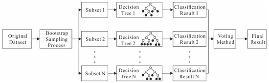
Figure 3. Schematic diagram of RF model principle [46].

Random Forest is an ensemble learning technique that improves prediction accuracy and robustness by constructing multiple decision trees and aggregating their predictions. The method introduces two forms of randomness during training: bootstrapping and the random selection of feature subsets. Specifically, Random Forest first samples from the original dataset with replacement to generate different training subsets for each tree; then, at each decision node, the algorithm does not consider all possible features for splitting but selects the best split feature from a randomly chosen subset of features. This strategy not only enhances the model’s generalization ability and reduces the risk of overfitting but also allows the model to effectively handle large datasets with high-dimensional feature spaces.

In this paper, positive samples consist of known mineral points, while negative samples are randomly generated within the quaternary deposits. The model splits the training and validation set in an 8:2 ratio, uses 100 decision trees, and evaluates based on the Gini index, with a minimum of 2 samples per leaf and at least 1 sample required to split a node.

4. Results and Discussion

For geochemical data, the correct approach to data processing is crucial as it can reveal the enrichment or depletion of elements, providing a direct basis for subsequent delineation of prospecting targets. Since the development of exploratory geochemistry techniques [6], there has been a significant evolution in the methods used to process geochemical data due to advancements in technology and the progression of time, becoming increasingly comprehensive and systematic. The approach has evolved from initial univariate analysis to multivariate analysis, and from earlier linear methods to current nonlinear and machine learning techniques. It is important to recognize that while older techniques are still valid, they may not suit contemporary needs; more refined data processing methods can greatly reduce costs and more clearly direct exploratory efforts.

4.1. Data Feature Description

All samples in this study area are fluvial sediments, with a general sampling layout of 1.0 per km², and a total of 2659 samples were collected. To enhance representativeness, samples are generally taken at river bends, behind boulders, in plunge pools, at the bottom of gullies, etc. Additional samples are collected 20–30 m upstream and downstream, or across the riverbed at 2–3 points, to form a composite original sample. The sampling medium includes silt, fine sand, etc., avoiding black organic matter, with a grain size of 250 μm. A total of 46 elements are analyzed, including Ag, As, Au, B, Ba, Be, Bi, Cd, Ce, Co, Cr, Cs, Cu, Hg, La, Li, Mn, Mo, Nb, Nd, Ni, Pb, Pr, Rb, Sb, Sc, Sn, Sr, Ta, Te, Th, Ti, Tl, U, V, W, Y, Zn, Zr, Al₂O₃, CaO, TFe₂O₃, K₂O, MgO, Na₂O, SiO₂. Testing methods are listed in Table 1. Sampling and analysis were conducted by Huabei Nonferrous (Sanhe) Yanjiao Central Laboratory Co., Ltd., Sanhe, China, with an internal quality pass rate of over 98% for all samples.

Table 1. Goulmima sample analysis methods.

Analysis Methods	Numbers	Elements
Graphite Furnace Atomic Absorption Spectrometry (GF-AAS)	1	Au
Inductively Coupled Plasma Mass Spectrometry (ICP-MS)	22	Nb, Th, Y, La, Ce, Pr, Nd, U, Ta, Mo, W, Cu, Pb, Co, Cd, Tl, Bi, Be, Cs, Te (Ni, Sc)
Inductively Coupled Plasma Atomic Emission Spectroscopy (ICP-AES)	22	Al2O3, Cr, TFe2O3, K2O, Li, MgO, Mn, Na2O, Ni, Sc, Sr, Ti, V, Zn, Rb (CaO, Ce, Nb, Cu, Th, Y, La)
X-ray Fluorescence Spectroscopy (XRF)	9	Ba, Zr, CaO, SiO2 (Sr, Al2O3, TFe2O3, MgO, Ti)
Emission Spectrometry (ES)	3	B, Sn, Ag
Hydride Generation—Atomic Fluorescence Spectroscopy (AFS)	3	As, Sb, Hg

For raw geochemical data, it is crucial to give due importance and handle it appropriately based on varying phenomena observed in the data. Therefore, it is essential for geologists to initially conduct a preliminary exploratory analysis of the raw data from the Goulmima area to gain an understanding of the data distribution characteristics. This initial analysis can help identify patterns, anomalies, and key statistical metrics that guide further detailed and specific treatments of the data.

From Table 2, it is pertinent to focus on the Coefficient of Variation (CV), where most elements do not exhibit high variability, except for Pb, Zn, Cd, Ba, Ag, and Hg. Notably, the element Pb has the highest CV (24.965), which relates with some Pb mineralization points in the northern part of the study area. Similarly, the element Zn also has a significant CV (6.620), which is consistent with its often co-occurrence with lead; the high variability coefficient for Cd (8.946) might be linked to local agricultural or industrial activities; Ag and Hg elements, which tend to migrate along faults, may be more concentrated in areas associated with faults, and the study area’s faults are primarily concentrated in the southern and northern parts, potentially resulting in high anomalies of these elements; Ba, being the primary element in barite, has its high concentration reflecting the abundance of barite mineralization points in the southern part of the study area.

Table 2. Statistical parameters of geochemistry elements content.

Element	Min	Q25	Q50	Q75	Max	Coefficient of Variation	Mean	Kurtosis	Skewness	Coefficient of Variation
Ag	0.031	0.056	0.070	0.100	9.650	0.217	0.092	1504.761	36.512	2.358
As	0.840	2.670	3.820	5.765	35.100	3.403	4.756	15.695	3.101	0.716
Au	0.260	0.540	0.660	0.760	18.500	0.426	0.672	1177.130	29.504	0.634
B	10.800	22.000	27.000	33.500	110.300	10.794	29.110	4.824	1.642	0.371
Ba	31.200	188.000	238.000	295.000	25,376.000	869.116	378.245	359.015	15.918	2.298
Be	0.250	0.420	0.580	0.830	2.480	0.314	0.663	0.977	1.083	0.473
Bi	0.030	0.054	0.071	0.093	0.390	0.036	0.078	5.320	1.642	0.453
Cd	0.030	0.069	0.110	0.160	76.400	1.577	0.176	2081.999	44.391	8.946
Ce	12.400	25.300	30.900	38.100	84.300	10.811	33.118	0.938	0.997	0.326
Co	1.940	4.720	6.050	7.870	26.000	2.806	6.640	3.342	1.426	0.423
Cr	10.100	28.000	34.800	43.700	141.000	13.336	37.023	5.541	1.550	0.360
Cs	0.480	1.220	1.690	2.500	11.600	1.093	1.992	4.709	1.549	0.549
Cu	3.320	9.040	11.700	15.200	118.000	5.959	12.966	39.177	3.346	0.460
Hg	0.004	0.011	0.015	0.023	0.780	0.030	0.021	349.959	15.747	1.429
La	6.840	13.500	16.400	20.000	44.600	5.244	17.281	1.125	0.951	0.303
Li	4.230	12.100	16.600	22.000	124.000	9.664	18.532	9.532	2.151	0.522
Mn	72.000	182.000	232.000	303.000	1058.000	117.829	260.015	3.912	1.625	0.453
Mo	0.190	0.290	0.330	0.430	2.980	0.162	0.385	50.404	4.882	0.420
Nb	2.660	6.800	8.130	9.660	23.200	2.295	8.409	1.626	0.797	0.273
Nd	5.850	11.700	14.200	17.300	38.200	4.435	14.924	0.819	0.848	0.297
Ni	3.810	10.100	13.300	17.200	60.200	6.397	14.472	3.705	1.455	0.442
Pb	3.500	8.710	12.000	17.200	50,603.000	995.725	39.884	2501.665	49.517	24.965
Pr	1.520	3.010	3.660	4.430	9.760	1.126	3.831	0.994	0.878	0.294
Rb	10.700	30.300	40.100	53.700	118.000	18.448	44.047	0.320	0.912	0.419
Sb	0.090	0.230	0.290	0.380	6.890	0.451	0.422	38.639	4.815	1.067
Sc	1.280	3.560	4.730	6.470	17.900	2.289	5.231	0.926	0.991	0.438
Sn	0.790	1.050	1.190	1.380	3.460	0.276	1.241	3.731	1.305	0.222
Sr	18.700	72.600	101.000	138.000	637.000	74.446	119.971	6.394	2.125	0.621
Ta	0.250	0.450	0.510	0.590	1.860	0.136	0.538	4.584	1.505	0.252
Te	0.006	0.015	0.021	0.030	0.086	0.010	0.023	1.398	0.820	0.426
Th	2.000	3.340	4.280	5.520	15.400	1.755	4.631	1.754	1.116	0.379
Ti	763.000	2229.500	2668.000	3223.500	11,952.000	901.186	2794.483	9.374	1.746	0.322
Tl	0.082	0.170	0.220	0.290	0.930	0.113	0.249	1.596	1.278	0.454
U	0.420	0.950	1.160	1.460	3.300	0.464	1.261	1.423	1.175	0.368
V	14.600	34.700	42.900	53.600	160.000	15.957	45.530	3.012	1.184	0.350
W	0.260	0.340	0.440	0.570	3.650	0.266	0.516	16.377	3.011	0.514
Y	4.090	8.915	11.200	14.100	31.300	4.094	11.952	0.565	0.871	0.343
Zn	6.890	22.700	31.400	43.600	14,671.000	307.900	46.511	1951.295	42.577	6.620
Zr	61.500	202.000	266.000	356.000	1147.000	126.006	291.655	3.408	1.399	0.432
Al2O3	0.740	3.190	4.390	6.170	15.560	2.202	4.865	0.059	0.774	0.453
CaO	0.620	4.320	6.630	11.340	30.250	5.136	8.330	-0.006	0.952	0.617
Fe2O3	0.570	1.560	2.010	2.700	8.560	0.884	2.181	2.558	1.099	0.405
K2O	0.270	1.010	1.290	1.710	4.120	0.548	1.410	0.479	0.858	0.388
MgO	0.140	1.000	1.400	1.960	9.980	1.107	1.659	11.834	2.811	0.668
Na2O	0.050	0.180	0.260	0.390	2.250	0.240	0.334	6.508	2.156	0.720
SiO2	34.190	60.670	69.860	77.735	117.010	12.413	68.721	−0.255	−0.251	0.181

Notes: the concentrations of Ag, Au, Bi, Cd, Hg, Sb, Ta, Te, Tl, and W are measured in parts per billion (10⁻⁹), oxides are measured in percentages (%), and other elements are measured in parts per million (10⁻⁶), coefficient of variation (CV) = standard deviation/mean.

In addition to the CV, by observing the skewness and kurtosis of elements, it is evident that some elements exhibit considerable skewness, which is typical for geochemical data due to the different degrees of accumulation of elements—typically presenting mostly low values with sporadic high values. These elements also have kurtosis values greater than the normal distribution standard of “3”, indicating that the data do not conform to a normal distribution. Geochemical data processing generally relies on classical mathematical models, such as multivariate statistical analysis, which first requires the data to approximate a normal distribution, especially when delineating geochemical anomalies. Geologists often use a method based on the mean plus standard deviation to define anomalies. However, non-normal distribution data can lead to the mean being skewed by extreme values, creating a significant difference between the mean and the median, which directly impacts the accuracy of geochemical anomaly classification. Therefore, after a preliminary analysis of data characteristics, it is considered necessary to subject the raw data to more refined processing.

4.2. Results of Compositional Data Analysis

4.2.1. Characteristics of Data After ilr Transformation

As seen from the characteristics displayed in Table 3, all elements show moderate kurtosis and skewness after undergoing ilr transformation. It is evident that there are no significant high-value peaks or skewness in the elements, suggesting that the transformed data essentially conforms to a normal distribution.

Table 3. Statistical characteristics table of data after ilr transformation.

Element	Min	Q25	Q50	Q75	Max	StdDev	Mean	Median	Kurtosis	Skewness
Ag	−5.292	−4.224	−4.055	−3.873	0.484	0.334	−4.035	−4.055	19.185	1.967
As	−1.275	−0.238	−0.061	0.142	1.593	0.321	−0.042	−0.061	1.795	0.542
Au	−2.849	−2.151	−1.922	−1.677	1.142	0.351	−1.898	−1.922	2.482	0.596
B	1.104	1.757	1.910	2.059	2.711	0.245	1.908	1.910	0.253	−0.017
Ba	2.282	3.947	4.129	4.327	8.170	0.478	4.196	4.129	10.621	2.358
Be	−2.690	−2.093	−1.960	−1.837	−1.168	0.182	−1.961	−1.960	−0.062	0.096
Bi	−4.847	−4.205	−4.100	−4.006	−2.872	0.198	−4.105	−4.100	3.701	0.528
Cd	−5.245	−4.005	−3.747	−3.439	2.130	0.505	−3.689	−3.747	11.098	1.631
Ce	1.138	1.958	2.051	2.144	2.580	0.143	2.048	2.051	2.030	−0.434
Co	−0.242	0.262	0.374	0.505	1.392	0.194	0.393	0.374	1.234	0.588
Cr	1.221	2.037	2.146	2.265	3.046	0.213	2.151	2.146	1.077	0.249
Cs	−1.595	−1.046	−0.901	−0.741	0.392	0.241	−0.880	−0.901	0.601	0.495
Cu	0.333	0.942	1.047	1.166	3.340	0.183	1.065	1.047	11.120	1.446
Hg	−7.039	−5.868	−5.630	−5.393	−1.852	0.408	−5.607	−5.630	7.204	1.297
La	0.144	1.313	1.403	1.495	1.891	0.144	1.396	1.403	6.539	−1.104
Li	0.848	1.250	1.356	1.507	2.781	0.224	1.399	1.356	1.690	1.018
Mn	3.358	3.984	4.066	4.180	5.166	0.169	4.093	4.066	2.359	0.902
Mo	−3.272	−2.627	−2.474	−2.314	−0.708	0.250	−2.461	−2.474	3.229	0.758
Nb	−0.063	0.535	0.658	0.801	1.597	0.210	0.675	0.658	0.863	0.436
Nd	0.407	1.166	1.255	1.335	1.812	0.128	1.249	1.255	1.385	−0.352
Ni	0.500	1.015	1.161	1.329	2.163	0.229	1.172	1.161	0.103	0.219
Pb	0.160	0.954	1.091	1.266	8.697	0.443	1.162	1.091	51.033	4.715
Pr	−0.962	−0.214	−0.115	−0.031	0.457	0.136	−0.124	−0.115	1.525	−0.448
Rb	1.491	2.207	2.301	2.403	2.835	0.159	2.302	2.301	0.646	−0.108
Sb	−3.564	−2.791	−2.642	−2.497	−0.132	0.407	−2.568	−2.642	3.596	1.655
Sc	−0.512	0.027	0.113	0.232	0.830	0.164	0.139	0.113	0.699	0.630
Sn	−2.224	−1.373	−1.257	−1.128	−0.307	0.200	−1.245	−1.257	0.765	0.229
Sr	2.241	2.965	3.156	3.455	5.135	0.419	3.248	3.156	0.581	0.899
Ta	−3.061	−2.290	−2.105	−1.905	−1.173	0.279	−2.096	−2.105	−0.114	0.100
Te	−6.047	−5.490	−5.351	−5.230	−4.262	0.201	−5.359	−5.351	0.764	0.052
Th	−0.828	−0.045	0.043	0.127	0.745	0.146	0.042	0.043	1.499	0.113
Ti	5.366	6.315	6.486	6.702	7.925	0.314	6.535	6.486	1.017	0.810
Tl	−3.614	−3.045	−2.943	−2.845	−2.254	0.171	−2.938	−2.943	0.776	0.291
U	−1.722	−1.359	−1.271	−1.188	−0.704	0.137	−1.269	−1.271	0.533	0.255
V	1.725	2.281	2.359	2.438	3.151	0.134	2.361	2.359	2.078	0.283
W	−3.017	−2.346	−2.236	−2.103	0.002	0.227	−2.199	−2.236	9.623	1.853
Y	0.233	0.939	1.011	1.086	1.491	0.120	1.011	1.011	1.110	−0.202
Zn	1.384	1.914	2.043	2.173	7.446	0.316	2.073	2.043	58.478	5.068
Zr	2.653	3.899	4.217	4.520	5.577	0.465	4.212	4.217	−0.141	−0.031
Al2O3	−0.871	−0.058	0.068	0.178	0.689	0.180	0.054	0.068	0.626	−0.396
CaO	−1.831	0.151	0.531	0.934	2.133	0.608	0.513	0.531	0.014	−0.327
Fe2O3	−1.224	−0.818	−0.747	−0.653	0.234	0.137	−0.732	−0.747	3.031	0.727
K2O	−2.061	−1.283	−1.177	−1.061	−0.479	0.180	−1.167	−1.177	0.699	0.175
MgO	−2.555	−1.369	−1.156	−0.859	0.711	0.391	−1.092	−1.156	1.278	0.842
Na2O	−3.948	−3.023	−2.764	−2.494	−1.316	0.408	−2.749	−2.764	−0.093	0.170
SiO2	1.436	2.488	2.818	3.162	4.037	0.474	2.818	2.818	−0.580	−0.032

Further observation of the data distribution characteristics after ilr transformation using box plots reveals that the transformed data are more normalized and concentrated in their spatial distribution (Figure 4). The box plots also show a more symmetric distribution of high and low extremes, better reflecting the trends in elemental anomalies. Therefore, we can conclude that the ilr data transformation significantly reduces the heterogeneity of the data structure, reduces skewness in the distribution, and aligns the data with the requirements of multivariate statistical analysis.

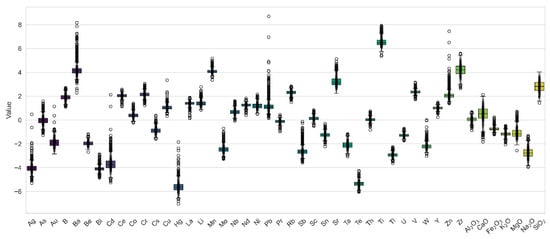
Figure 4. Boxplot of data after ilr transformation.

4.2.2. Principal Component Biplot

Figure 5 sequentially presents the biplots of the original data, the data transformed by ilr transformation, and analyzed using principal component analysis (PCA) and robust principal component analysis (RPCA) for the first two principal components, PC1 and PC2. The biplots of the original data (Figure 5a–c) show a pronounced “leaning” trend, indicating that the data still exhibit the closure effect [36,47]. However, after the ilr transformation and subsequent PCA analysis, the variables are “unfolded”, and the overall presentation is radial, effectively eliminating the closure effect.

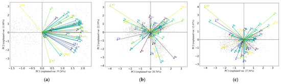
Figure 5. Principal component biplot, (a): PCA of the raw data; (b): PCA of data after ilr transformation; (c): RPCA of data after ilr transformation.

In the biplot of the original data, except for SiO₂, all other elements show positive loadings on PC1, which complicates the display of interrelationships among elements through the biplot. However, in the biplots after ilr transformation, whether classical or robust, elements are more evenly distributed across the four quadrants formed by PC1 and PC2, allowing for the determination of relationships among elements based on the angles between them.

For example, in the classical biplot, elements Pb and Zn are both located in the third quadrant with a small angle between them, indicating their similarity. The oxides CaO and MgO are found in the second quadrant, also with a small angle between them, primarily present in silicate minerals in igneous and metamorphic rocks such as olivine, pyroxene, amphibole, and garnet. A high content of MgO is usually associated with ultrabasic rocks, which may originate from mantle materials. Meanwhile, a higher content of CaO may indicate the presence of carbonate rocks or rocks rich in feldspar. At the same time, elements Co and Ni are also located in the second quadrant, primarily occurring in olivine and other ultramafic minerals, reflecting their association with mantle source areas. Particularly, the element Sr is also in the second quadrant and has a significant length (large proportion), because Sr commonly combines with calcium in nature to form strontianite (SrCO₃), thus it is closely related to CaO; Sodium oxide (Na₂O) usually does not exist independently as a mineral but is a component of many silicate minerals such as feldspar and plagioclase. In igneous rocks, the content of barium and sodium can reflect the source and evolution of the magma. For example, during the magma differentiation process, early crystallizing feldspar might enrich sodium, while later feldspar or other silicate minerals might enrich barium.

Although classical PCA after ilr transformation provides some explanations for elemental correlations, certain issues remain (Figure 5b). For example, in the fourth quadrant, elements or oxides like Ba, Sb, and Na₂O, which are major contributors, show strong correlations (with small angles between them). However, this contradicts the geochemical properties of these elements. Ba tends to enrich more easily in sedimentary environments, is chemically stable, and has poor mobility, whereas Sb is more active in reducing environments, with some volatility and mobility. Additionally, Mo, Sn, and W are high-temperature elements and should show good correlations, however, Mo and Sn appear in the first quadrant, while W is located in the fourth quadrant. What is the cause of such a significant difference?

This discrepancy occurs because classical PCA is easily influenced by outliers. While the ilr-transformed data closely follows more symmetrical distributions, certain elements may still behave irregularly, which is a common phenomenon in exploration geochemistry. Therefore, it is convenient to use RPCA to mitigate this risk. The results of RPCA are overall similar to those of classical PCA, but there are still noticeable differences. In the RPCA results, although Pb and Zn remain at the negative load end of PC1, they have shifted from the third quadrant to the second. For PC1, this shift has minimal impact, but PC2, Pb, and Zn, which were positive in classical PCA, have become negative in RPCA. Ba and Sb are also separated, no longer belonging to the same quadrant, which aligns more closely with geological patterns. High-temperature elements Mo, Sn, and W are all grouped in the first quadrant, indicating a closer relationship.

In conclusion, it is more reasonable to analyze the ilr-transformed data using RPCA, and selecting PC1 and PC2 from the RPCA results for further processing is the appropriate next step.

4.3. Results of Multifractal Analysis

Geological historical periods are prolonged processes, and mineralization typically occurs in multiple stages, causing geochemical data to follow a mixed distribution rather than a normal distribution [37]. The Spectrum-Area (S-A) fractal method can effectively separate the background and anomalies, significantly narrowing the target area for exploration. Considering that preliminary explorations in the study area have already identified several barite and lead-zinc mineralization points, and that barite and lead-zinc minerals often coexist, with copper frequently appearing as a secondary mineral in lead-zinc deposits, and considering the multiple pyrite mineralizations found in the Goulmima area, we have selected Ba, Pb, Zn, Cu, and TFe₂O₃ along with PC1 and PC2 derived from compositional data transformation for S-A fractal analysis. The fitting results are shown in Figure 6.

Figure 6. Spectrum-energy density (S) and area (A) plot. (a): element Ba, (b): element Cu, (c): Oxide Fe₂O₃, (d): element Pb, (e): element Zn, (f): principal component PC1, (g): principal component PC2.

The fitting results for various elements (oxides) as well as PC1 and PC2 are quite satisfactory, ensuring that the R² values are above 0.8. By setting the line segment cut-off value as the threshold, we filter out noise and background, and then use Fourier inverse transformation to generate anomaly maps; similarly, we can filter out noise and anomalies to obtain the background map (Figure 7). In Figure 7, for the column of geochemical anomaly maps on the left, we used the basic inverse distance weighting method for interpolation, with a grid size of 100 and a fixed search radius of 1200.

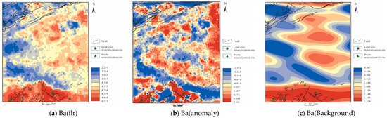
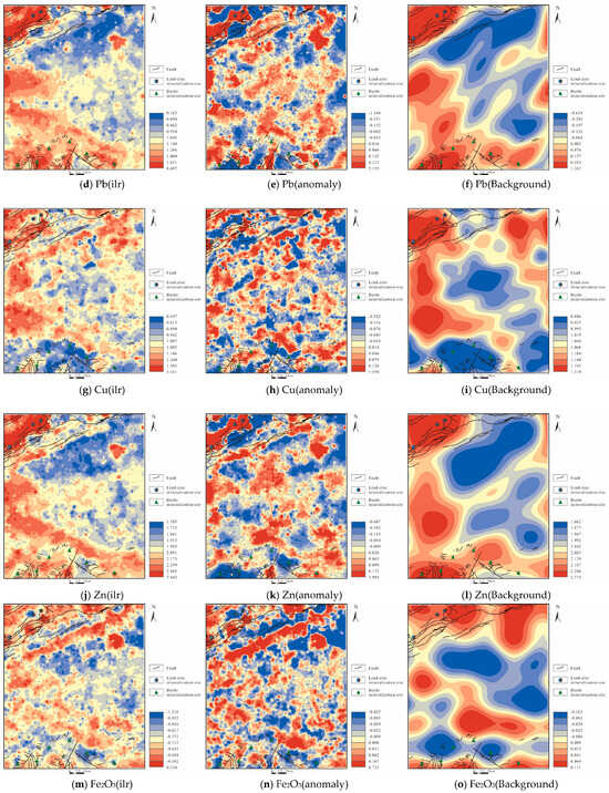
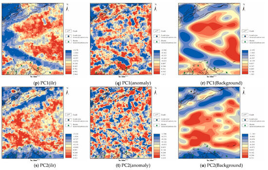
Figure 7. Geochemical maps of elements: (a,d,g,j,m,p,s) after ilr transformation; (b,e,h,k,n,q,t) anomalies decomposed by S-A; (c,f,i,l,o,r,u) background decomposed by S-A.

From Figure 7, it can be observed that the S-A anomaly decomposition significantly diminishes the anomalous background of the study area, thereby accentuating the anomalies in other regions that were previously overshadowed by high background values. For instance, the Ba element showed a large area of anomalies in the southern part prior to the S-A analysis. After fractal processing, the area of anomalies has been reduced, and a band-like anomaly distribution in the central part has been highlighted, along with some localized weak anomalies.

From Figure 7, it is apparent that there is little correlation between Ba and Pb, and their anomaly distribution patterns are also inconsistent. As seen in the biplot (Figure 5c), Ba and Pb almost display a 180° relationship, indicating that their modes are nearly opposite. Although it was mentioned earlier that barite and lead-zinc minerals typically coexist, this is usually in hydrothermally related deposits. However, the lead-zinc deposits in this study area are of the MVT type, which might explain some differences with barite occurrences. Observations of the geochemical anomaly map of Ba and the anomalies and background maps decomposed by S-A reveal that high-concentration anomalies of Ba are primarily concentrated in the northern part of the study area, a region with extensive volcanic rock distribution. This could be due to rhyolites or andesites, types of extrusive rocks that are often rich in elements brought from the mantle source area, including Ba. Ba might also become enriched in these extrusive rocks during volcanic eruptions through rapid crystallization or by coexisting with other minerals. Thus, the distribution model of Ba differs from other elements.

For the elements Cu, Pb, and Zn, both the geochemical anomaly maps post-ilr transformation and the subsequent anomaly and background maps processed through S-A fractal analysis are very similar. The high-value areas (red regions) in the geochemical anomaly maps of Cu, Pb, and Zn are largely consistent with the distribution of the Jurassic strata in the northern part of the study area. This reflects their similar geochemical behaviors. Moreover, from the biplot (Figure 5c), it can be observed that Pb and Zn are located in the second quadrant, with a very small angle between them, indicating a high degree of similarity, which aligns with the coexistence characteristics of lead and zinc ores. Meanwhile, Cu, as an associated mineral, appears in the third quadrant in the biplot with a certain angle from Pb and Zn but still falls under the negative loading of PC1, indicating a relationship with Pb and Zn, albeit not very close. Instead, Cu has a closer relationship with Fe, likely because both are chalcophile elements, and although iron may also form under oxidizing conditions, in this study area, it is primarily associated with pyrite mineralization, suggesting that Cu and Fe together indicate a predominantly reducing environment dominated by sulfides.

Regarding PC1 and PC2, PC1 mainly focuses on the background map, where the northern part of the background displays distinct high and low values along faults, but there is also a blue zone in the southern part. Comparing with other geochemical anomaly maps, almost all are oriented NW in this location, and the corresponding area in the geological map is largely composed of Quaternary (Q) deposits, suggesting the possibility of a significant NW-oriented deep fault in this area. Observing the biplot (Figure 5c), the positive end of PC1 is mainly characterized by elements such as Mo, Sn, Ti, W, U, reflecting the high-temperature hydrothermal conditions of the mineralization period, whereas the negative loading includes CaO, MgO, Pb, Zn, etc., indicating a sedimentary environment completely different from the hydrothermal setting, typical of the main formation environment for MVT-type lead-zinc deposits. Similarly, PC2’s background in the southern blue area indicates a geological setting in the southern part of the study area that includes both extrusive and intrusive rocks.

4.4. Geological Information Extraction

Although MVT-type lead-zinc deposits are primarily sedimentary in nature, necessary faults serve as a foundation for the source of mineralizing substances, thus, quantifying these faults helps to better understand the potential locations of the deposits.

In ArcGIS, faults can be analyzed using Euclidean distance, which is not constrained by the size of grid cells and does not require calculating the relationship between buffer radii and the distribution of mining points. Instead, it expresses the distance between faults and mining points in a continuous numerical format, retaining more information to the greatest extent (Figure 8).

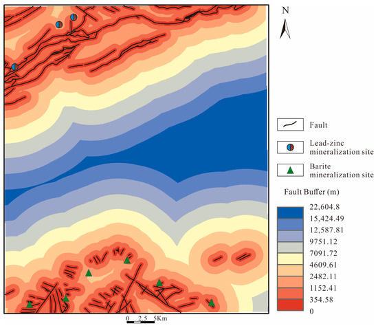
Figure 8. Fault Buffer Euclidean Distance Map.

After the faults have been quantitatively extracted, they can be used as a geological attribute evidence layer in the prediction model for computation.

4.5. Prediction and Target Area Delineation

4.5.1. RF Prediction Results

Due to its inherent parallel characteristics and good model interpretability, the Random Forest (RF) algorithm is widely used across various application fields. Unlike typical “black box” models, the Random Forest algorithm can provide a ranking of variable importance and the partial dependencies between variables. This feature allows for the identification and explanation of critical predictive factors, making it particularly effective in mineral resource prediction.

In this study, TIFF images are used as evidence layer inputs, with the study area’s boundary defined and the grid cell size set at 100 × 100, size 477 × 557. The chosen evidence layers include the S-A decomposed anomaly and background maps of Ba, Cu, Pb, Zn, Fe₂O₃, PC1, and PC2, as well as Fault Buffer.

After training with labeled samples, the resulting Receiver Operating Characteristic (ROC) curve (Figure 9a) achieves an Area Under the Curve (AUC) value of 0.946, indicating excellent performance on the training set. Finally, the trained model is used to predict mineralization zones across the entire study area (Figure 10).

Figure 9. (a) ROC curve; (b) success rate curve.

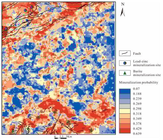
Figure 10. RF prediction results.

The prediction results from the RF model indicate that high probability areas are primarily located near existing mineralization points. Additionally, new extensive red areas are displayed in the northern part of the study area, suggesting potential for future mineral exploration. When correlated with the geological map, this region corresponds to the junction between the Jurassic and Cretaceous strata and is intersected by two northeast (NE) oriented faults, providing favorable conditions for mineralization.

Furthermore, plotting the percentage of mining points against the cumulative percentage of area reveals that all known mining points are contained within the top 20% of the ranked areas. This demonstrates a high concentration of mineralized regions, underscoring the model’s practicality in effectively identifying key mineralized areas.

4.5.2. Target Area Delineation

To facilitate the delineation of target areas, we employed the Concentration-Area (C-A) fractal technique to divide the target area into three zones: outer, middle, and inner. The cut-off values were calculated using a bi-logarithmic plot, ensuring an R² above 0.75 for better line segment fitting. Typically, the first line segment represents the outer zone anomalies (low anomalies), the second line segment represents the middle zone anomalies (moderate anomalies), and the third segment represents the inner zone anomalies (high anomalies). Overall, the C-A fractal does not alter the distribution shape of the anomalies but provides a clear division of the prediction results into high, medium, and low zones. Compared to Figure 10, the high-probability red areas in Figure 11, after C-A fractal processing, are more concentrated, which is beneficial for directing subsequent exploration efforts.

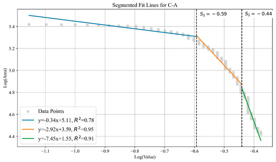
Figure 11. C-A fractal bi-logarithmic plot.

Based on the distribution of the high-potential red areas and the existing mining point information, two prospecting target areas have been delineated within the study area (Figure 12). Target I is located in the northern part of the study area, where two NE-oriented faults intersect. All elements show anomalies at this location, and it lies at the junction between the Jurassic and Cretaceous strata, forming an excellent structural plane for mineralization with significant potential. Target II is located near the southern part of the study area. Although no faults are shown in this location on the geological map, Cu, Pb, and Zn all exhibit exceptionally high anomaly values here, with the anomaly direction extending NW. This suggests the potential presence of an undiscovered fault, providing favorable conditions for mineralization.

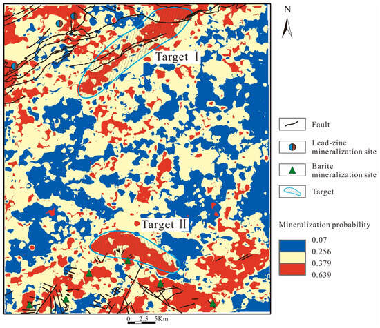
Figure 12. Target area map delineated after C-A fractal analysis.

4.5.3. Interpretability Analysis

The core concept of SHAP (SHapley Additive exPlanations) indeed originates from the Shapley value in co-operative game theory. In co-operative game theory, the Shapley value is used to measure the contribution of each participant in a coalition or co-operation, ensuring fair distribution of profits. SHAP cleverly introduces this concept into the interpretation of machine learning models, quantifying the contribution of each feature to the prediction outcome. Through SHAP, we can provide a precise explanation for each prediction in a Random Forest model, demonstrating the degree to which each feature contributes to the predictive result.

As shown in Figure 13, the fault buffer makes the largest contribution to the model, followed by the element Ba. This result aligns with our expectations since faults are essential channels for hydrothermal migration, thus constituting a necessary condition for mineralization, especially at intersections of faults. Additionally, the Goulmima area is predominantly characterized by lead-zinc deposits, hence the concentration of Pb is a crucial criterion for mineral prospecting, and the same logic applies to Ba. Regarding PC2, principal component analysis reduces all factors into a few major components representing all information; thus, compared to PC1, PC2 carries less weight and consequently shows the least significance in the SHAP plot.

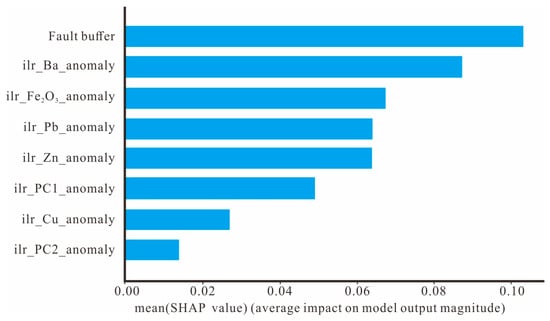
Figure 13. Average impact bar chart of SHAP values.

5. Conclusions

This paper is based on preprocessing geochemical data using Compositional Data Analysis (CoDA) and multifractal methods, and employs a Random Forest model to optimize mineral prospecting targets in the Goulmima area, yielding the following conclusions:

(1)

Data Transformation and Analysis: By comparing the statistical characteristics and biplots of the original data with those after the isometric log-ratio (ilr) transformation, it was observed that the ilr transformation resolved the closure problem inherent in the original data and provided a symmetric distribution of elements. This suggests that data post-ilr transformation better explain the spatial structure of the elements.

(2)

Using ilr-transformed data, both classical PCA and RPCA analyses were performed. The results suggest that RPCA provides more reliable outcomes, and two distinct combinations of elements were identified. PC1 primarily includes elements such as Mo, Sn, Ti, W, and U, indicative of a high-temperature hydrothermal environment, while PC2 comprises elements like CaO, Pb, and Zn, which are typical of a low-temperature mineralization environment. These combinations of elements align well with the multi-stage mineralization geological background of the study area.

(3)

The application of the S-A (Spectrum-Area) multifractal model effectively identified and separated the anomaly-background distribution characteristics of geochemical data elements and their combinations within the study area. Subsequently, the isolated anomalies were combined with fault buffer distances to serve as evidence layers for predictive mineral prospecting.

(4)

The C-A fractal model was utilized to further delineate high, medium, and low probability areas in the prediction results, ultimately defining two prospective target areas for mining.

In summary, the study effectively enhanced the interpretability of geochemical data and the precision of mineral prospecting predictions through appropriate data preprocessing and analytical methods. It demonstrates the value of combining Compositional Data Analysis, multifractal methods, and machine learning technologies in geochemical exploration.

References

- Bonham-Carter, G.F. Geographic Information Systems for Geoscientists: Modelling with GIS, 1st ed.; Computer Methods in the Geosciences; Pergamon: Kidlington, UK, 2002; ISBN 978-0-08-042420-0. [Google Scholar]
- Porwal, A.; Carranza, E.J.M. Introduction to the Special Issue: GIS-Based Mineral Potential Modelling and Geological Data Analyses for Mineral Exploration. Ore Geol. Rev. 2015, 71, 477–483. [Google Scholar] [CrossRef]
- Carranza, E.J.M. Analysis and Mapping of Geochemical Anomalies Using Logratio-Transformed Stream Sediment Data with Censored Values. J. Geochem. Explor. 2011, 110, 167–185. [Google Scholar] [CrossRef]
- Wang, X. Landmark Events of Exploration Geochemistry in the Past 80 Years. Geol. China 2013, 40, 322–330. [Google Scholar]
- Parsa, M.; Sadeghi, M.; Grunsky, E. Innovative Methods Applied to Processing and Interpreting Geochemical Data. J. Geochem. Explor. 2022, 237, 106983. [Google Scholar] [CrossRef]
- Wang, X. A Decade of Exploration Geochemistry. Bull. Mineral. Petrol. Geochem. 2013, 32, 190–197. [Google Scholar]
- Zuo, R.; Carranza, E.J.M. Support Vector Machine: A Tool for Mapping Mineral Prospectivity. Comput. Geosci. 2011, 37, 1967–1975. [Google Scholar] [CrossRef]
- Xiong, Y.; Zuo, R. Recognition of Geochemical Anomalies Using a Deep Autoencoder Network. Comput. Geosci. 2016, 86, 75–82. [Google Scholar] [CrossRef]
- Zuo, R.; Wang, J. ArcFractal: An ArcGIS Add-In for Processing Geoscience Data Using Fractal/Multifractal Models. Nat. Resour. Res. 2020, 29, 3–12. [Google Scholar] [CrossRef]
- Zuo, R.; Carranza, E.J.M.; Wang, J. Spatial Analysis and Visualization of Exploration Geochemical Data. Earth-Sci. Rev. 2016, 158, 9–18. [Google Scholar] [CrossRef]
- Agterberg, F.P. Combining Indicator Patterns in Weights of Evidence Modeling for Resource Evaluation. Nat. Resour. Res. 1992, 1, 39–50. [Google Scholar] [CrossRef]
- Cheng, Q. BoostWofE: A New Sequential Weights of Evidence Model Reducing the Effect of Conditional Dependency. Math. Geosci. 2015, 47, 591–621. [Google Scholar] [CrossRef]
- Harris, D.; Zurcher, L.; Stanley, M.; Marlow, J.; Pan, G. A Comparative Analysis of Favorability Mappings by Weights of Evidence, Probabilistic Neural Networks, Discriminant Analysis, and Logistic Regression. Nat. Resour. Res. 2003, 12, 241–255. [Google Scholar] [CrossRef]
- Singer, D.A.; Kouda, R. Classification of Mineral Deposits into Types Using Mineralogy with a Probabilistic Neural Network. Nat. Resour. Res. 1997, 6, 27–32. [Google Scholar] [CrossRef]
- Harris, D.; Pan, G. Mineral Favorability Mapping: A Comparison of Artificial Neural Networks, Logistic Regression, and Discriminant Analysis. Nat. Resour. Res. 1999, 8, 93–109. [Google Scholar] [CrossRef]
- Chen, Y.; Wu, W. Mapping Mineral Prospectivity Using an Extreme Learning Machine Regression. Ore Geol. Rev. 2017, 80, 200–213. [Google Scholar] [CrossRef]
- Xiong, Y.; Zuo, R.; Carranza, E.J.M. Mapping Mineral Prospectivity through Big Data Analytics and a Deep Learning Algorithm. Ore Geol. Rev. 2018, 102, 811–817. [Google Scholar] [CrossRef]
- Cracknell, M.J.; Reading, A.M. Geological Mapping Using Remote Sensing Data: A Comparison of Five Machine Learning Algorithms, Their Response to Variations in the Spatial Distribution of Training Data and the Use of Explicit Spatial Information. Comput. Geosci. 2014, 63, 22–33. [Google Scholar] [CrossRef]
- Rahmati, O.; Pourghasemi, H.R.; Melesse, A.M. Application of GIS-Based Data Driven Random Forest and Maximum Entropy Models for Groundwater Potential Mapping: A Case Study at Mehran Region, Iran. CATENA 2016, 137, 360–372. [Google Scholar] [CrossRef]
- Rodriguez-Galiano, V.F.; Chica-Olmo, M.; Chica-Rivas, M. Predictive Modelling of Gold Potential with the Integration of Multisource Information Based on Random Forest: A Case Study on the Rodalquilar Area, Southern Spain. Int. J. Geogr. Inf. Sci. 2014, 28, 1336–1354. [Google Scholar] [CrossRef]
- Carranza, E.J.M.; Laborte, A.G. Random Forest Predictive Modeling of Mineral Prospectivity with Small Number of Prospects and Data with Missing Values in Abra (Philippines). Comput. Geosci. 2015, 74, 60–70. [Google Scholar] [CrossRef]
- McKay, G.; Harris, J.R. Comparison of the Data-Driven Random Forests Model and a Knowledge-Driven Method for Mineral Prospectivity Mapping: A Case Study for Gold Deposits Around the Huritz Group and Nueltin Suite, Nunavut, Canada. Nat. Resour. Res. 2016, 25, 125–143. [Google Scholar] [CrossRef]
- Zhang, S.; Xiao, K.; Carranza, E.J.M.; Yang, F. Maximum Entropy and Random Forest Modeling of Mineral Potential: Analysis of Gold Prospectivity in the Hezuo–Meiwu District, West Qinling Orogen, China. Nat. Resour. Res. 2019, 28, 645–664. [Google Scholar] [CrossRef]
- Hariharan, S.; Tirodkar, S.; Porwal, A.; Bhattacharya, A.; Joly, A. Random Forest-Based Prospectivity Modelling of Greenfield Terrains Using Sparse Deposit Data: An Example from the Tanami Region, Western Australia. Nat. Resour. Res. 2017, 26, 489–507. [Google Scholar] [CrossRef]
- Carranza, E.J.M.; Laborte, A.G. Data-Driven Predictive Modeling of Mineral Prospectivity Using Random Forests: A Case Study in Catanduanes Island (Philippines). Nat. Resour. Res. 2016, 25, 35–50. [Google Scholar] [CrossRef]
- Cavin, L.; Tong, H.; Boudad, L.; Meister, C.; Piuz, A.; Tabouelle, J.; Aarab, M.; Amiot, R.; Buffetaut, E.; Dyke, G.; et al. Vertebrate Assemblages from the Early Late Cretaceous of Southeastern Morocco: An Overview. J. Afr. Earth Sci. 2010, 57, 391–412. [Google Scholar] [CrossRef]
- Lebedel, V.; Lezin, C.; Andreu, B.; Wallez, M.-J.; Ettachfini, E.M.; Riquier, L. Geochemical and Palaeoecological Record of the Cenomanian–Turonian Anoxic Event in the Carbonate Platform of the Preafrican Trough, Morocco. Palaeogeogr. Palaeoclimatol. Palaeoecol. 2013, 369, 79–98. [Google Scholar] [CrossRef]
- Filzmoser, P.; Hron, K.; Templ, M. Applied Compositional Data Analysis: With Worked Examples in R; Springer Series in Statistics; Springer: Cham, Switzerland, 2018; ISBN 978-3-319-96422-5. [Google Scholar]
- Liu, Y.; Cheng, Q.; Xia, Q.; Wang, X. Application of Singularity Analysis for Mineral Potential Identification Using Geochemical Data—A Case Study: Nanling W–Sn–Mo Polymetallic Metallogenic Belt, South China. J. Geochem. Explor. 2013, 134, 61–72. [Google Scholar] [CrossRef]
- Zuo, R. Identification of Geochemical Anomalies Associated with Mineralization in the Fanshan District, Fujian, China. J. Geochem. Explor. 2014, 139, 170–176. [Google Scholar] [CrossRef]
- Vera, P.-G.; Juan, J.E.; Raimon, T.-D. Modeling and Analysis of Compositional Data; Statistics in Practice; John Wiley & Sons: Hoboken, NJ, USA, 2015; ISBN 1-118-44306-3. [Google Scholar]
- Nazarpour, A.; Omran, N.R.; Paydar, G.R.; Sadeghi, B.; Matroud, F.; Nejad, A.M. Application of Classical Statistics, Logratio Transformation and Multifractal Approaches to Delineate Geochemical Anomalies in the Zarshuran Gold District, NW Iran. Geochemistry 2015, 75, 117–132. [Google Scholar] [CrossRef]
- Piepel, G.F. The Statistical Analysis of Compositional Data. Technometrics 1988, 30, 120–121. [Google Scholar] [CrossRef]
- Filzmoser, P.; Hron, K.; Reimann, C. Principal Component Analysis for Compositional Data with Outliers. Environmetrics 2009, 20, 621–632. [Google Scholar] [CrossRef]
- Zuo, R. Identification of Weak Geochemical Anomalies Using Robust Neighborhood Statistics Coupled with GIS in Covered Areas. J. Geochem. Explor. 2014, 136, 93–101. [Google Scholar] [CrossRef]
- Aitchison, J.; Greenacre, M. Biplots of Compositional Data. J. R. Stat. Soc. Ser. C Appl. Stat. 2002, 51, 375–392. [Google Scholar] [CrossRef]
- Cheng, Q.; Agterberg, F.P.; Ballantyne, S.B. The Separation of Geochemical Anomalies from Background by Fractal Methods. J. Geochem. Explor. 1994, 51, 109–130. [Google Scholar] [CrossRef]
- Cheng, Q.M.; Agterberg, F.P.; BonhamCarter, G.F. A Spatial Analysis Method for Geochemical Anomaly Separation. J. Geochem. Explor. 1996, 56, 183–195. [Google Scholar] [CrossRef]
- Cheng, Q. Mapping Singularities with Stream Sediment Geochemical Data for Prediction of Undiscovered Mineral Deposits in Gejiu, Yunnan Province, China. Ore Geol. Rev. 2007, 32, 314–324. [Google Scholar] [CrossRef]
- Cheng, Q.; Agterberg, F.P. Singularity Analysis of Ore-Mineral and Toxic Trace Elements in Stream Sediments. Comput. Geosci. 2009, 35, 234–244. [Google Scholar] [CrossRef]
- Ghasemzadeh, S.; Maghsoudi, A.; Yousefi, M.; Mihalasky, M.J. Stream Sediment Geochemical Data Analysis for District-Scale Mineral Exploration Targeting: Measuring the Performance of the Spatial U-Statistic and C-A Fractal Modeling. Ore Geol. Rev. 2019, 113, 103115. [Google Scholar] [CrossRef]
- Afzal, P.; Alghalandis, Y.F.; Khakzad, A.; Moarefvand, P.; Omran, N.R. Delineation of Mineralization Zones in Porphyry Cu Deposits by Fractal Concentration–Volume Modeling. J. Geochem. Explor. 2011, 108, 220–232. [Google Scholar] [CrossRef]
- Chen, G.; Cheng, Q. Singularity Analysis Based on Wavelet Transform of Fractal Measures for Identifying Geochemical Anomaly in Mineral Exploration. Comput. Geosci. 2016, 87, 56–66. [Google Scholar] [CrossRef]
- Cheng, Q.; Agterberg, F.P. Multifractal Modeling and Spatial Statistics. Math. Geol. 1996, 28, 1–16. [Google Scholar] [CrossRef]
- Daya, A.A.; Afzal, P. A Comparative Study of Concentration-Area (C-A) and Spectrum-Area (S-A) Fractal Models for Separating Geochemical Anomalies in Shorabhaji Region, NW Iran. Arab. J. Geosci. 2015, 8, 8263–8275. [Google Scholar] [CrossRef]
- Breiman, L. Random Forests. Mach. Learn. 2001, 45, 5–32. [Google Scholar] [CrossRef]
- Tang, R.; Sun, L.; Ouyang, F.; Xiao, K.; Li, C.; Kong, Y.; Xie, M.; Wu, Y.; Gao, Y. CoDA-Based Geo-Electrochemical Prospecting Prediction of Uranium Orebodies in Changjiang Area, Guangdong Province, China. Minerals 2023, 14, 15. [Google Scholar] [CrossRef]
Disclaimer/Publisher’s Note: The statements, opinions and data contained in all publications are solely those of the individual author(s) and contributor(s) and not of MDPI and/or the editor(s). MDPI and/or the editor(s) disclaim responsibility for any injury to people or property resulting from any ideas, methods, instructions or products referred to in the content. |
© 2025 by the authors. Licensee MDPI, Basel, Switzerland. This article is an open access article distributed under the terms and conditions of the Creative Commons Attribution (CC BY) license (https://creativecommons.org/licenses/by/4.0/).