Mitigating Supply Chain Disruptions in Plywood Manufacturing by Deadline Reordering

Abstract

Disruptions in supply networks have caused many logistical and planning challenges in the last few years. The previous predictability of the shipping times of raw materials changed drastically due to various global issues, which affected many production areas, including the wood industry. This work is motivated by a case study of a Central European plywood production facility, where supply-side disruptions caused difficulties in meeting deadlines for downstream companies of the construction and furniture industry. As a result, the objective of production planners shifted towards mitigating the financial burden caused by cancellation penalties. Three MILP (Mixed-Integer Linear Programming) models and a genetic algorithm were developed to tackle the scheduling of a plywood production plant with raw material shipments and order deadlines. The novelty of the considered problem lies in the flexibility of swapping order deadlines from the same client, which was inspired by the real-life deals of the aforementioned company. The methods were tested on 120 benchmark instances of different sizes generated from real industrial data. The genetic algorithm terminated within 60 s for all instances and found the optimal or best-known solution in 71 of 80 short-horizon instances, while also remaining efficient on larger 30-day cases. As the solution approach is not specific to plywood production, it can be applied to scheduling problems in other fields as well, where similar disruptions can develop, and the production process features are covered by the Multi-Mode Resource-Constrained Project Scheduling Problem class.

1. Introduction

1.1. Motivation

Inventory management is a key task in most production facilities. There is an inherent tradeoff between storage costs and the robustness of the production plan. In today’s competitive market, companies tend to reduce inventory (and thus costs) as much as possible, and this transition has accelerated due to the generally good reliability of supply chains. As a result, the production chains of most products omit larger, longer-term inventories, and a new order appears immediately on the whole chain. These chains are typically cost-optimized with little or no reserves, making them susceptible to external disturbances. Moreover, their global reach, i.e., spanning over distant geographical locations, renders the supply chains extremely vulnerable. Recent years have shown that natural disasters, pandemics [1], or even human errors on bottleneck shipping routes [2,3] can have a major impact on the supply chains of most of today’s goods.

Most companies in the middle of a supply chain face a new challenge: the outbound shipments of products cannot all be satisfied due to the lateness or cancellation of inbound shipments of raw materials. The penalties on the inbound side often do not cover the penalties caused by the cancellation on the outbound side, not to mention the lost opportunity cost. Thus, companies do their best to mitigate these supply disturbances to reduce costs, dampening the ripple effect of cancellations.

Plywood manufacturing is an excellent example of an industry in such a position. At the facility investigated by the authors, the general goal was to minimize canceled orders and the associated penalties. In addition to general rescheduling, decision-makers had another available option: renegotiating deadlines with downstream clients. As transportation logistics are usually fixed, in most cases, the only freedom that remained was reordering the shipments of the same client, in a way that can be better satisfied with the altered supply situation. Clients were also interested in finding a feasible solution this way, as a canceled order (or canceled supply shipment on their side) would cause similar issues for them as well. As a result, allowing swapped shipments was often preferred by the clients as the associated penalty was significantly lower than that of cancellation.

To the best of our knowledge, the combination of order cancellation and deadline permutation studied here has not been addressed in the optimization literature. This paper aims to present MILP formulations and a metaheuristic algorithm that address this issue, and to investigate how much this new objective function and decision freedom increases the difficulty of this rescheduling problem. The results are exploratory, as there are no literature models to compare with, due to the novelty of the problem definition itself. However, two different MILP models (and some variants of those) and a genetic algorithm are presented and tested, in order to validate their solutions and compare their efficiency.

1.2. Plywood Production Process

Plywood is an engineered wood belonging to the family of manufactured boards, which includes, among others, medium-density fiberboard (MDF), oriented strand board (OSB), and particle board (chipboard). More precisely, plywood is a wood-based composite material manufactured from thin layers (plies) of wood veneer that are glued together, with adjacent layers having their wood grain rotated up to 90 degrees to one another. In general, the thickness of the layers is not greater than 7 mm. The layer order is symmetric and the board consists of a minimum of three layers. Because of their frequent usage, physical and chemical properties of the plywood have been extensively investigated [4,5,6].

Plywood is widely used for different purposes and can be separated into two general classes: (a) construction and industrial plywood, and (b) decorative plywood [7]. Plywood can be used for building purposes, furniture-making, or sports equipment manufacturing (e.g., table tennis rackets). Therefore, as a raw material, it plays an important role in the industry, and its contribution to sustainability is also high because of the carbon storage potential [8].

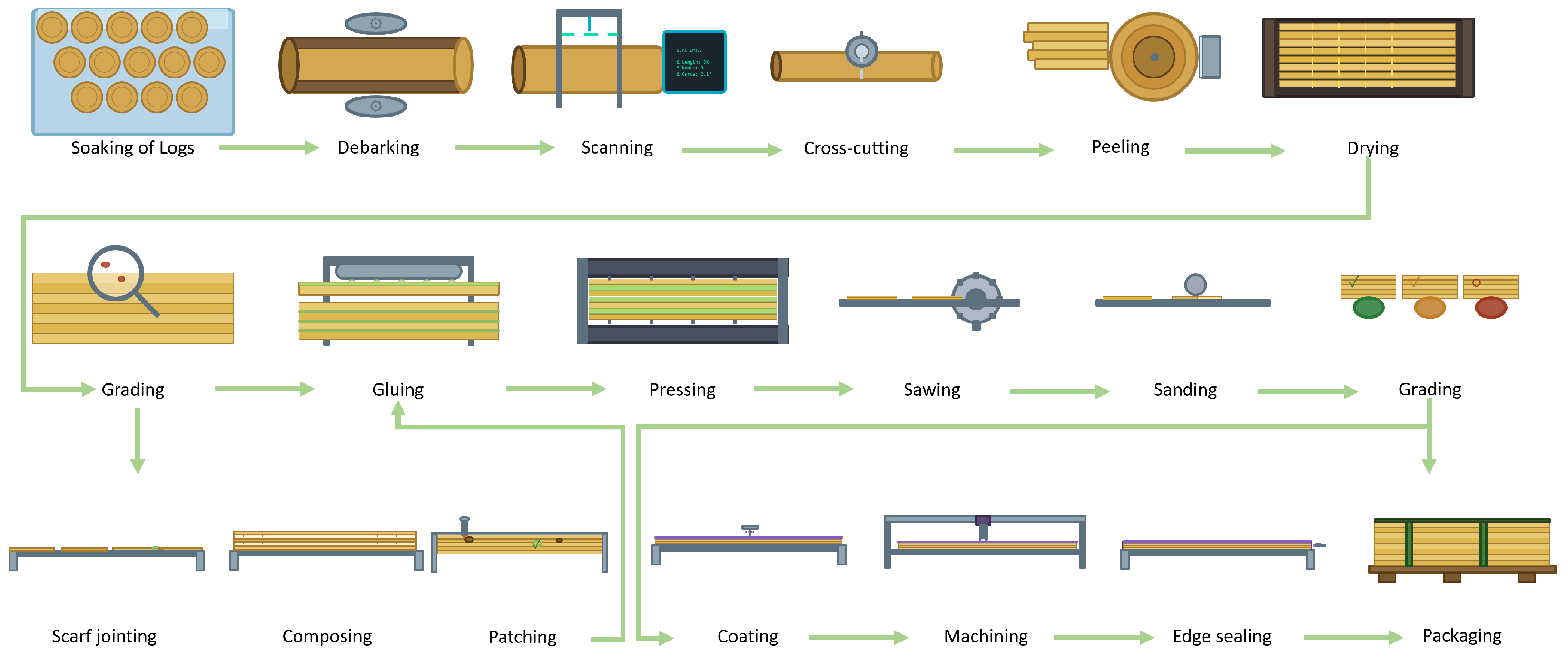
Plywood production consists of two major phases that include many operations. The first phase is veneer manufacturing, and the second phase is plywood manufacturing. In addition to these two phases, further processing can be done because several byproducts of these phases are used as raw material in pulp and paper production or as biofuel in power generation plants [9,10]. Different phases and operations of the general plywood production process are demonstrated in Figure 1.

The logs are stored in the log yard under soaking to prevent degradation. Before the logs are cut and peeled, the bark must be removed. An important step to avoid damages later is the scanning procedure to detect metal parts in the logs. Debarked logs are moved to the cross cutter. The size of the logs is dependent on the finished panel size and the grain direction. The next production step is peeling, where veneer is produced. The veneers must be dried for several reasons. After drying, the veneers are graded. Small defects can be repaired, e.g., open knots in birch wood can be plugged in.

The next step is gluing the surface of the veneers to prepare the plywood for pressing. They are then placed on top of an unglued veneer, so that the stack alternates: glued, unglued, glued, unglued, and so on. When the veneers are glued, high pressure is applied in order to bind the glue. After pressing, the boards are trimmed by sawing. When the geometry is ready, the surface of the plywood is sanded by an industrial sander.

The last step for raw plywood is grading, which is a part of quality control. During grading, the final product is assessed and prepared for packaging. If a coating is applied on the surface of the plywood, the next steps are connected to that. The last step is packaging, where the finished plywood panels are stacked up and banded together, and the necessary marking and labeling are also performed.

1.3. Production Planning

Several operations research problems in plywood mills have been investigated in the past [11,12,13]. Nowadays, from the economic, efficiency, and sustainability perspectives, plywood production can be in focus. Particularly production planning and scheduling play an important role. In recent years, the topic has been investigated through several case studies and mathematical models. In their case study, Laamanen [14] examined the role of production planning in building up a company’s competitive edge. Borthakur and Nath [15] investigated the Systematic Layout Planning technique in order to increase the productivity of the manufacturing. Paarma [16] studied the Sales and Operations Execution planning process that aims to balance the short-term demand and supply. Mäkinen et al. [17] formulated a MILP for solving the scheduling problem of bonding and coating machines.

Related optimization problems appear at other primary processing stages of the wood industry as well, mainly in sawmilling and panel production. Scheduling models over a planning horizon in sawmills have to consider decisions such as equipment operation, personnel assignment and choosing the right cutting pattern for each log [18]. Selecting appropriate cutting patterns for logs is especially important, and a flexible way of generating these—adapting to log availability—can increase production efficiency [19]. Mathematical models can be augmented by real-world information sources, such as detailed log geometry obtained from scanning technologies, to further improve the decision-making process of pattern generation and assignment [20].

As optimization problems arising in production planning and the wood industry in general are inherently complex, heuristic and metaheuristic approaches are often applied to obtain good-quality solutions within a reasonable computational time [21]. Genetic algorithms (GAs) are metaheuristic methods that have proven to be effective for production planning and scheduling problems. Recent applications of GA in the wood industry include production scheduling in the panel industry [22], solving cutting stock decision problems [23], and panel layout optimization [24].

Plywood scheduling is a challenging and time-consuming task for production planners. Multiple customer orders, different wood processing machines and material usage have to be simultaneously taken into account. In addition to the processes in plywood mills, one of the biggest influences on proper production planning is the experience of the production planner. This work aims to apply mathematical and metaheuristic methods to the problem, based on approximate production data from a Central European plywood mill.

1.4. Scheduling with Order Acceptance and Due Date Assignment

In production planning, machine scheduling models such as flow shop and job shop scheduling are the most commonly used approaches [25] regardless of the considered optimization objectives. This is mostly because the biggest bottlenecks in availability are expensive industrial equipment units, and the supply of other resources, e.g., operators, raw materials, is often assumed to be always sufficient. However, the problem investigated in this paper considers multiple scarce resources: machines, operators, and raw materials. Extending traditional machine scheduling models to incorporate resource constraints efficiently would be a difficult task.

Order acceptance scheduling (OAS) is a variant of machine scheduling where production capacities are limited, and decision-makers have to select which subset of the given jobs to process [26]. These decisions are usually made with the objective of maximizing revenue or minimizing penalties from refused jobs or tardiness. OAS has been studied for many variations of the machine scheduling problems, including capacitated job shop [27] and parallel machines [28]. The key difference between OAS and the problem studied in this paper is that OAS assumes fixed deadlines, and either accepts an order, in some cases with generalized due date [29], or rejects it completely.

Due date assignment (DDA) is another variant of machine scheduling where setting the due dates is part of the scheduling decisions instead of being input parameters [30,31]. In many cases, DDA models are categorized as a type of OAS problem [26]. DDA models have been combined with order rejection/cancellation [32], and studies have considered jobs with multiple deadlines [33]. While DDA focuses on setting the deadlines together with the scheduling decisions, the present paper addresses a situation where previously fixed deadlines must be either permuted or canceled, and the scheduling decisions must be made accordingly.

1.5. Mitigation of Supply Chain Disruptions and Renegotiation of Due Dates

Mitigating the effect of unforeseen disruptions in supply chains is a widely studied area with proactive and reactive stages. Reactive approaches encompass recovery methods that are implemented after a disruption has occurred [34,35], and are the most relevant with regards to this paper. However, reactive methods take the original plan as a starting point, and aim to find a new feasible solution with minimal deviation from the original one. In the case of our studied problem, we create a completely new production plan with the consideration of the disrupted supply information.

Snyder et al. [36] reviewed operations research and management science models for the mitigation of supply chain disruptions. They identified three main categories of mitigation strategies: inventory control, sourcing/demand flexibility, facility location and interaction with external partners. Based on their description, our problem cannot be categorized directly into any of these, as we consider a combined scheduling and modification of demand-side deadlines. Rescheduling flow shop production layouts was studied by Katragjini et al. [37], who presented simple rescheduling methods for three disruptions scenarios: machine breakdowns, new job arrivals and job-ready time variations.

Renegotiation of due dates is a common practice in many industries, especially to mitigate the effects of supply chain disruptions. However, these practices have only been studied from a strategic and behavioral standpoint. Plambeck and Taylor [38] studied renegotiation possibilities of various contract terms in supply chains, and conclude that these can greatly increase firms’ investments and profits in the case of correctly designed contracts. Moodie [39] investigated various strategies for agreeing on prices and due dates, and showed that due date quotation strategies benefit from negotiation. It can be seen that while negotiation strategies in supply chains under disruption have been studied from a behavioral and strategic perspective, and various reactive strategies mitigating disruption have been modeled via MILP, the integrated optimization of production scheduling and permuting order deadlines remains unexplored.

1.6. MRCPSP

Section 1.4 showed that the problem studied in this paper is not a straightforward application of an existing OAS or DDA machine scheduling model. Instead, it was modeled as a Resource-Constrained Project Scheduling Problem (RCPSP) in order to incorporate the management of multiple resources for production steps. The RCPSP is a well-known, actively studied problem class [40,41,42,43], which entails scheduling activities requiring different quantities from resources with finite capacities. The precedence relations between activities are given by a directed acyclic graph, defining a partial ordering of the activities. A more general problem class is the Multi-mode RCPSP (MRCPSP), where activities can have multiple possible operation modes, that may differ in the types and quantities of required resources, and durations [44,45]. In this class, non-renewable resources, such as consumed materials, can be present too, which renders certain mode combinations of activities infeasible, regardless of their timing.

MRCPSP can be regarded as a generalization of the flexible job shop problem: machines are renewable resources, and heterogeneous machines can be modeled as alternative operation modes. As a more general model, its solution is often more computationally difficult, especially if the number of operation modes for the activities is high. However, it can inherently handle operations requiring multiple resources (machines and human operators), and limited availability of raw materials as well.

For small-sized problems, there are several RCPSP approaches in the literature, which guarantee optimality, based on mathematical and constraint programming models, and the S-graph framework [46]. One promising modeling approach is the event-based formulation, proposed by Koné et al. [47] for the RCPSP, and extended to the MRCPSP by Chakrabortty et al. [48]. The authors showed that this formulation is not as sensitive to long activity durations as the discrete-time models used by most of the other approaches. This is an important aspect of the investigated plywood manufacturing process, as its steps may require several hours because of the high processing volumes. The S-graph framework was extended to MRCPSP by Ősz and Hegyháti [49], including the modeling of time-varying resource capacities, which can be utilized for handling raw material shipments, scheduled maintenances, or work shift imbalances. However, this approach is limited to small-sized problems, as its computational needs grow significantly with the introduction of more operations.

The most common objective of MRCPSP variants is the minimization of the completion time. When deadlines are considered, they are either used as soft constraints, and lateness is minimized [50,51], or the cost of meeting these deadlines is minimized [52]. While there have been no studies linking OAS to MRCPSP [53], only a few studies have investigated due dates in RCPSP [54,55], and they follow a similar approach to their machine scheduling counterparts. MRCPSP was studied with time-dependent resource costs and capacities by Rodríguez-Ballesteros et al. [45], and with resource limitations and supply time constraints by Xie et al. [56].

It can be seen from the above sections that while the problem studied in this paper is related to both OAS and DDA, it is not a direct application of either of them. In OAS, the key decision is whether to accept or reject an order, but accepted orders typically keep their original, fixed deadlines. In DDA, deadlines are decision variables that are determined together with the scheduling decisions. This is in contrast to the problem studied in this paper, where deadlines may only be swapped with each other if they belong to the same customer, linking the decisions of order acceptance and deadline reordering. Moreover, OAS and DDA models are mostly machine scheduling problems that do not consider multiple resources and temporal non-renewable raw material supply. This positions our problem as an integration of the above problem classes, an MRCPSP with order acceptance and customer-specific deadline swapping.

To the best of our knowledge, this paper is the first to address the above-mentioned integrated scheduling problem that combines:

• scheduling a multi-resource plywood production with non-renewable raw materials arriving over time under disrupted supply conditions;
• the option of swapping deadlines of orders from the same client to mitigate the effect of resource shortage.

The main contributions of the paper are:

• the formulation of this new deadline-swapping scheduling problem;
• the development of three MILP models and a genetic algorithm to solve it;
• the computational comparison of these methods on instances generated based on real industrial data.

2. Problem Definition

The aim of this research is to mitigate the economic burden of a plywood production plant in a volatile and unreliable supply market via internal process scheduling and demand-side contract alterations. While demand-side contract deadlines are usually determined by taking into account the time requirements of the supply of necessary raw materials, events in the last few years have shown that global supply chain networks are often optimized for cost-effectiveness, disregarding robustness. Many companies were unable to meet the deadlines of their customers due to a delayed supply of raw materials, and plywood production plants were no exception.

Before these market disturbances, the production planners’ main concern was often the most efficient utilization of equipment to maximize throughput. However, recently, many of them had to shift their priorities to avoid late deliveries when supply was stalled. Planners had to decide which contracts to break to minimize the costs stemming from late fees and penalties. The focus shifted from “take on as many orders as possible” to “cancel as few as possible”. The bottleneck became the supply of raw materials instead of production equipment.

Planners had several options at their disposal to mitigate the financial damage of supply-side volatility. Internal rescheduling is always an option; however, the potential results are limited if supply-side lateness is significant, which it often was. To the benefit of these plants, many contracts allow potential reordering of the deliveries for the same client, e.g., if a client has two deliveries with different products and deadlines, it is more beneficial for both sides to satisfy them in reverse order than to cancel one or both of them. The latter would potentially force the client to cancel their contracts further in the supply chain. Thus, for an agreed financial compensation the company may swap the orders, and deliver them accordingly. This deadline change, permutation, may occur between two or more orders, as long as they belong to the same client. Unlike optimizing for simple tardiness, this option also has the benefit of not disrupting the transportation plans.

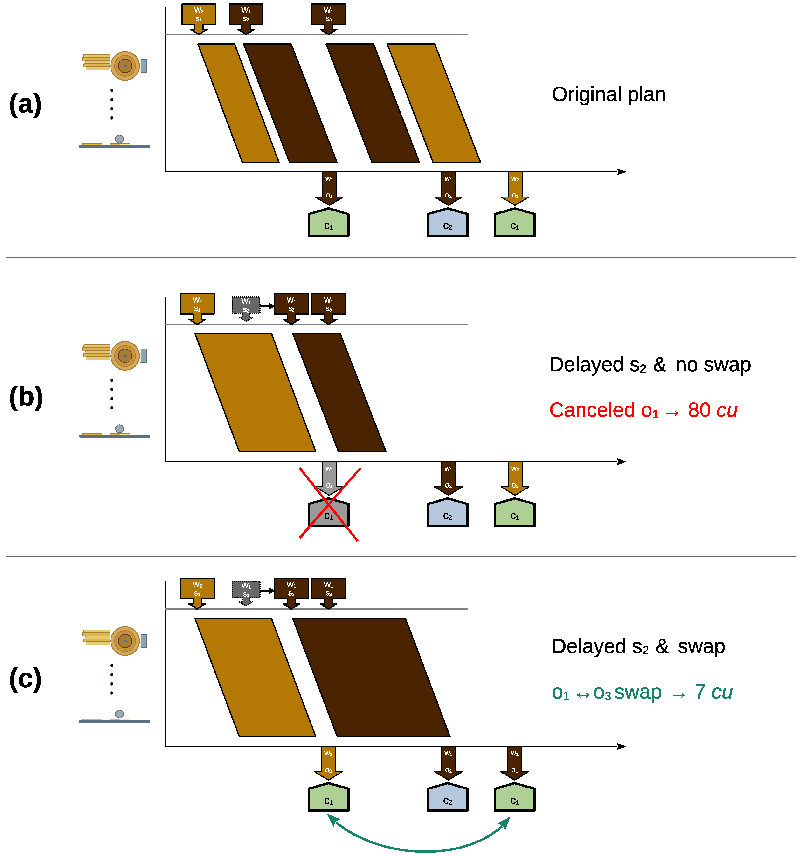
Figure 2 illustrates the advantages of allowing such a rescheduling, if available. In this example, 2 clients ($c_1$-green and $c_2$-blue) placed 3 orders ($o_1$, $o_2$ and $o_3$) of two different wood types ($w_1$-dark and $w_2$-light). In the original plan based on 3 shipments of wood logs ($s_1$–$s_3$), this could have been satisfied by the production line. However, shipment $s_2$ gets delayed, rendering order $o_1$ impossible to satisfy, resulting in its cancellation cost of 80 cu. However, if client $c_1$ allows the swapping of the two orders, $o_3$ can be satisfied by the deadline of $o_1$, and there remains enough time for the other two orders after the two dark-wood shipments. This alteration only costs the company 7 cu.

In summary, the investigated problem is to swap and/or cancel orders and reschedule the internal processes of a plywood production facility so that the penalties for order alterations are kept minimal.

The considered optimization problem can be partitioned into two main parts: data and options related to orders, and internal scheduling data.

From the market side, the company has a set of clients, each with a collection of contracts for deliveries. A delivery entails products and quantities with a deadline. The planner can cancel any contract, resulting in a major fee, or swap the deadlines of two or more orders from the same client for a (probably smaller) predetermined price. While the cost of cancellation is usually defined in the contract, the frequent need to swap orders is an emerging phenomenon, and there are no set or agreed rules on the cost, which may depend on the client, the importance of the order, the difference between the deadlines, etc. Currently, the cost or option of such changes is the basis of per-case negotiations. In this paper, the cost is assumed to be the sum of fixed costs assigned to each specific deadline alteration. More general cost functions, e.g., an arbitrary fixed cost for each permutation and cancellation combination could easily be addressed with additional continuous variables and constraints. This formulation, however, is still powerful enough to properly model some common practical scenarios, for example:

• If the client is really flexible with the order of the arrival of its orders, all swapping costs could be set to 0.
• If a specific order cannot be swapped at all, the related swapping costs could be set to a sufficiently large value to prevent that.
• If—based on downstream clients for example—swaps may be allowed only between distinct subsets of orders even for the same client, it can also be achieved by setting the cost of the forbidden swaps sufficiently high.

The planning and execution of delivery logistics are not homogeneous across clients: some operate their own fleet of delivery vehicles, while others leave that to subcontractors. Moreover, some contracts may entail shipment organization and costs as well. In the current investigation, such details are not considered, and it is assumed that planning of deliveries is outside of the scope of the production planner. It is also assumed that deliveries of the same client have equal capacity, so swapping orders does not cause feasibility issues. However, delivery vehicles still have limited capacity, so if the delivery time of one order is changed to the time of another, the original must be canceled or changed to another time too.

In this study, the following steps are considered in the production of each order: peeling, drying, patching (if needed), pressing, sawing, and sanding.

At each stage, several machines may be available to perform the tasks, which may be utilized in a parallel fashion. Each machine requires a number of people for its proper operation.

Peeling requires wood supplied by inward shipments.

2.1. Formal Problem Definition of Inputs

Formally, the problem can be defined with the sets and parameters listed in

Table 1. Nomenclature for input sets and parameters.

Sets
C	set of clients
E	set of equipment units
$E_k$	set of equipment units for the production step $k\in K$
$E_{a,m}$	set of equipment units used for activity $a\in A$ in mode $m\in M_a$
K	$=\{\mathtt{pl},\mathtt{dr},\mathtt{pt},\mathtt{pr},\mathtt{sw},\mathtt{sn}\}$ set of production steps
O	set of orders
$O_c$	$\subseteq O$ set of orders of client $c\in C$
$O^P$	$\subseteq O$ set of orders that require patching ($\mathtt{pt}$)
S	$=\{1,2,\dots ,|S\left|\right\}$ set of shipments
$S_w$	$\subseteq S$ set of shipments with wood type $w\in W$
W	set of wood types
Parameters
$c_o$	$\in C$ the client of order $o\in O$
$f_e^w$	$\in {\mathbb{R}}_0^{+}$ flow rate of equipment unit $e\in E$ [$m^3/h$]
$o_a$	$\in O$ the order associated with activity $a\in A$
$p_o^c$	$\in {\mathbb{R}}_0^{+}$ price / cost of cancellation of order $o\in O$ [$cu$] (cu = cost units)
$p_{o,o^{\prime }}^s$	$\in {\mathbb{R}}_0^{+}$ price / cost of moving the deadline of order o to $t_{o^{\prime }}^d$ with $o,o^{\prime }\in O$ and $c_o=c_{o^{\prime }}$ [$cu$]
$q^m$	$\in \mathbb{N}$ number of manual operators at the facility [$ea.$]
$q_e^m$	$\in \mathbb{N}$ number of manual operators needed to operate equipment $e\in E$ [$ea.$]
$q_o^r$	$\in {\mathbb{R}}_0^{+}$ required quantity of $w_o$ in order $o\in O$ [$m^3$]
$q_s^w$	$\in {\mathbb{R}}_0^{+}$ mass of shipment $s\in S$ [$m^3$]
$t_s^a$	$\in \mathbb{N}$ arrival time of shipment $s\in S$ [h]
$t_o^d$	$\in \mathbb{N}$ original deadline of order $o\in O$ [h]
$w_o$	$\in W$ wood type of order $o\in O$
$w_s$	$\in W$ wood type of shipment $s\in S$

and described below. The complete list of notations can be found in Appendix A.

Let C denote the set of clients, and O the set of orders. $O_c$ denotes the orders from client $c\in C$, and $c_o$ refers to the client of order $o\in O$. Naturally, $O_c$ sets are disjoint, and ${\bigcup }_{c\in C}{O}_c=O$. Set $O^P$ denotes the set of orders that require patching.

The original deadline of order $o\in O$ is denoted by $t_o^d$, and its cancellation would impose $p_o^c$ cost units (cu). Moving the deadline of order o to that of another order of the same client $o^{\prime }$, i.e., to $t_{o^{\prime }}^d$ costs $p_{o,o^{\prime }}^s$. Changes appear in permutations, and the total cost is the sum of the costs for each individual deadline alteration.

The set W denotes the set of wood types that are used as raw materials. $w_o$ indicates the wood type of order $o\in O$ and $q_o^r$ refers to the total mass of that order.

S denotes the set of raw material shipments. Shipment $s\in S$ has the mass of $q_s^w$ of wood type $w_s\in W$ and arrives at $t_s^a$. For simpler notation, the set of shipments bringing wood type $w\in W$ is denoted by $S_w$. Without loss of generality, it is assumed that $S=\{1,2,\dots ,|S\left|\right\}$ and $t_s^a\le t_{s+1}^a$ for all $s=1,2,\dots ,\left|S\right|-1$.

The set of production steps is denoted by $K=\{\mathtt{pl},\mathtt{dr},\mathtt{pt},\mathtt{pr},\mathtt{sw},\mathtt{sn}\}$, where $\mathtt{pl}$, $\mathtt{dr}$, $\mathtt{pt}$, $\mathtt{pr}$, $\mathtt{sw}$, $\mathtt{sn}$ refers to peeling, drying, patching, pressing, sawing, sanding, respectively. For simpler notation, we indicate production order by the → relation as follows:

$$\mathtt{pl}\to \mathtt{dr}\to \mathtt{pt}\to \mathtt{pr}\to \mathtt{sw}\to \mathtt{sn}$$

Parameter $q^m$ gives the number of manual operators, and $E_k$ refers to the set of equipment units (machines) used at the production step $k\in K$. $E_k$ sets are disjoint, and the set of all equipment units is $E={\bigcup }_{k\in K}{E}_k$. Equipment units can work on any order regardless of their wood type.

For each equipment unit $e\in E$, $q_e^m$ indicates the number of operators required for its proper operation, and $f_e^w$ denotes the flow rate of that unit, i.e., the mass of material it can process per hour, which is independent of the wood type.

2.2. Problem Superclass

The structure of the internal process of the plywood production facility is a very specific, sequential recipe with parallel executions, and three types of resources: wood (intermediates), equipment units, and manual operators.

While this study considers the six significant steps of plywood production, the proposed model should be general enough to allow straightforward inclusion of further steps in future research. Moreover, other segments of the production industry with different process structures probably had similar issues in recent years. Thus, the model proposed below addresses a more general process structure, while keeping the market-related parameters as described above.

The production process follows a sequential recipe, which can be described by a directed acyclic graph, so structurally, the process adheres to the rules of the standard RCPSPs. The production steps, however, may be carried out by several equipment units in parallel, which could be modeled by $2^n-1$ modes if n equipment units are available at a stage. Thus, if the logs were present at the beginning of the considered time horizon, the plywood production process could be considered as a standard MRCPSP with some non-renewable resources.

The proposed models tackle a more general problem class, which entails both the standard MRCPSP and the problem defined in Section 2.1. This problem superclass can be interpreted in two ways: either as a generalized MRCPSP, in which non-renewable resources are not available at the beginning of the time horizon and some activities have deadlines, can be canceled or swapped, and contribute to the overall cost to be minimized, or as a generalization of the plywood process scheduling problem, in which the recipes can have a more general MRCPSP structure.

2.3. Mapping Plywood Production Data to MRCPSP Input

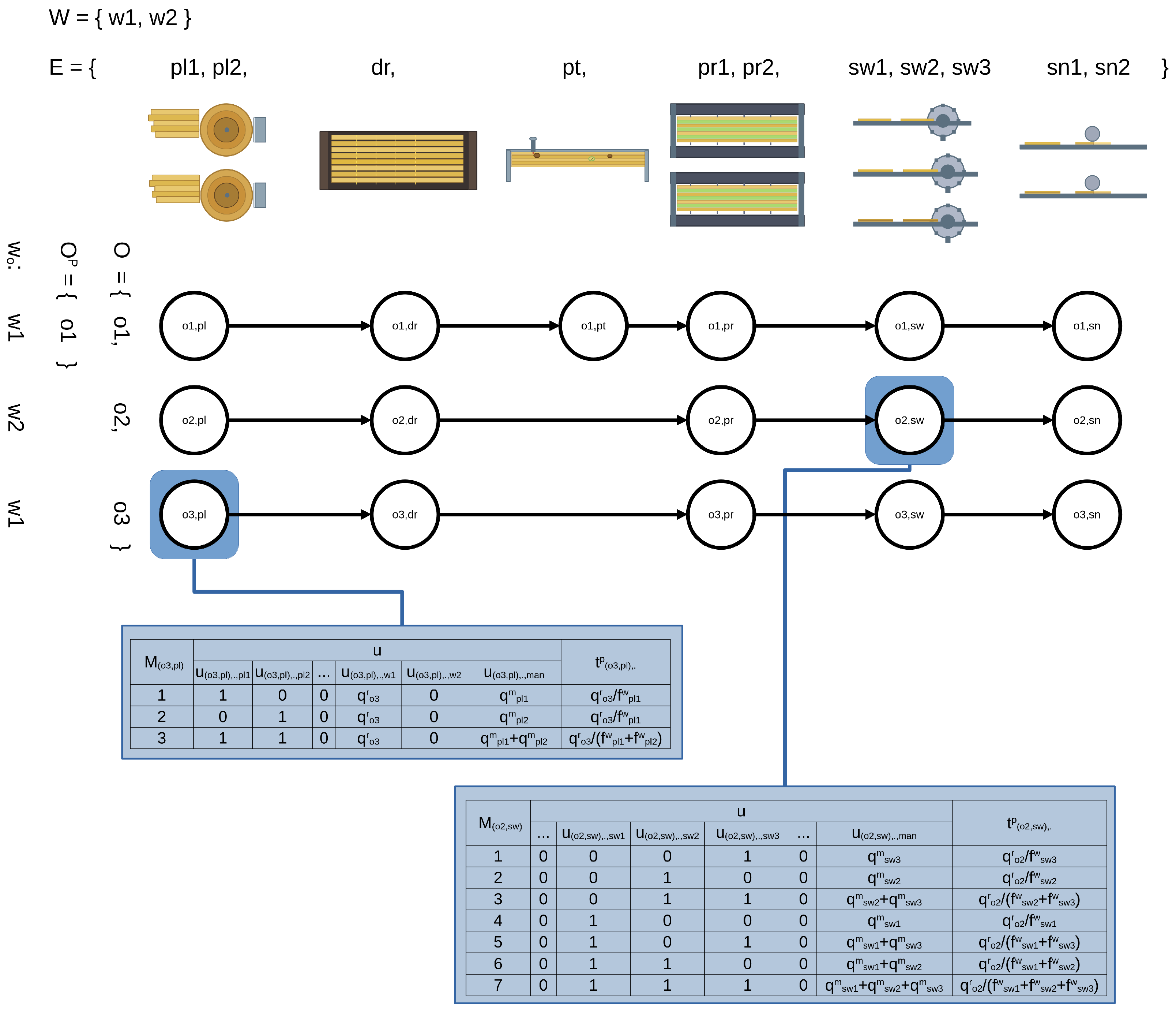
As MRCPSP is well-known in the industry, and the proposed models are based on MRCPSP as well, production-related data are transformed into the more general MRCPSP formulation. The overview of the mapping is shown in

Table 2. Mapping problem input to MRCPSP.

Plywood Production	MRCPSP
Production steps	Activities
Wood logs	Non-renewable resources
Equipment units and operators	Renewable resources
Different/parallel unit assignment options	Multiple operation modes

. Market-related data, i.e., sets C, O, $O_c$, S, and parameters $c_o$, $p_o^c$, $p_{o,o^{\prime }}^s$, $t_s^a$, $t_o^d$ remain unchanged.

Formally, the MRCPSP inputs listed in

Table 3. Nomenclature for the MRCPSP part of the superclass.

Sets
A	set of activities
$M_a$	set of operation modes for activity $a\in A$
P	$\subseteq A\times A$ set of precedences among activities
R	set of renewable resources
V	set of non-renewable resources
Parameters
$a_o^l$	$=(o,\mathtt{sn})\in A$ the last activity of order $o\in O$
$k_a$	$\in K$ the production step associated with activity $a\in A$
$o_a$	$\in O$ the order associated with activity $a\in A$
$v_s$	$\in V$ the non-renewable delivered in shipment $s\in S$
$q_r^c$	$\in {\mathbb{R}}_0^{+}$ available capacity of renewable resource $r\in R$ [$ea.$]
$t_{a,m}^p$	$\in {\mathbb{R}}_0^{+}$ processing time of activity $a\in A$ in mode $m\in M_a$ [h]
$u_{a,m,r}$	$\in {\mathbb{R}}_0^{+}$ resource $r\in R\cup V$ used by activity $a\in A$ in mode $m\in M_a$ [$m^3$] or [$ea.$]

are defined based on the sets and parameters of plywood production as follows.

Non-renewable resources are denoted by the set V, and in plywood production only the wood logs are non-renewable:

$$V:=W$$

Renewable resources, denoted by R, are the equipment units and manual operators:

$$R:=E\cup \left\{\mathtt{man}\right\}$$

where $\mathtt{man}$ indicates the manual operators.

Resources are usually indexed by r (or by v if it is known to be non-renewable). Instead of $w_s$, the notation $v_s$ will be used.

The available capacity of each renewable resource $r\in R$ is denoted by $q_r^c$. For equipment units, the capacity is 1, as there are no identical machines, and for manual labor, it is equal to the number of operators, $q^m$:

$$q_r^c:=\left\{\begin{array}{cc}1& \mathrm{if}r\in E\hfill \\ q^m& \mathrm{if}r=\mathtt{man}\hfill \end{array}\right.$$

The activities, denoted by A, are the production steps of the plywood process for each order:

$$A:=O\times \left(K\setminus \left\{\mathtt{pt}\right\}\right)\cup O^P\times \left\{\mathtt{pt}\right\}$$

For simpler notation, $a_o^l:=(o,\mathtt{sn})$ denotes the last activity of order $o\in O$. Also, the order and production step part of $a\in A$ is denoted by $o_a$ and $k_a$, respectively, that is, $a=(o_a,k_a)$.

The precedence relation $P\subseteq A\times A$, between the activities, is given as follows:

$$\begin{array}{ccc}\hfill P& :=& \left\{\left((o,k),(o,k^{\prime })\right)\mid (o,k),(o,k^{\prime })\in A\wedge k\to k^{\prime }\right\}\hfill \\ & \cup & \left\{\left((o,\mathtt{dr}),(o,\mathtt{pr})\right)\mid o\in O\setminus O^P\right\}\hfill \end{array}$$

For each $a\in A$ the set of operation modes denoted by $M_a$ is given by the possible machine combinations. Each non-empty combination defines a different operation mode:

$$M_a:=1,2,\dots ,\left|\mathcal{P}\left(E_{k_a}\right)\right|-1$$

The set of equipment units used in operation mode m of activity a is denoted by $E_{a,m}$:

$$\left\{E_{a,m}\mid m\in M_a\right\}=\mathcal{P}\left(E_{k_a}\right)\setminus \varnothing$$

The processing time for activity $a\in A$ in mode $m\in M_a$ is denoted by $t_{a,m}^p$. It is equal to the order quantity divided by the combined flow rate of the machines present in mode m:

$$t_{a,m}^p:={\displaystyle \frac{q_{o_a}^r}{{\displaystyle \sum _{e\in E_{a,m}}}{f}_e^w}}$$

Finally, the usage of resource $r\in R\cup V$ of activity $a\in A$ in mode $m\in M_a$ is denoted by $u_{a,m,r}$ and calculated as follows:

$$u_{a,m,r}:=\left\{\begin{array}{cc}{q}_o^r& \mathrm{if}r=w_o\mathrm{and}{k}_a=\mathtt{pl}\hfill \\ {\displaystyle \sum _{e\in E_{a,m}}}{q}_e^m& \mathrm{if}r=\mathtt{man}\hfill \\ 1& \mathrm{if}r\in E_{a,m}\hfill \\ 0& \mathrm{otherwise}\hfill \end{array}\right.$$

Wood logs are consumed only by the first step, which is peeling. The number of required operators is the sum of the operator counts for each machine used. For machine resources, the usage is 1 for each machine used for the mode.

Figure 3 illustrates how the plywood production process is reduced to an MRCPSP problem.

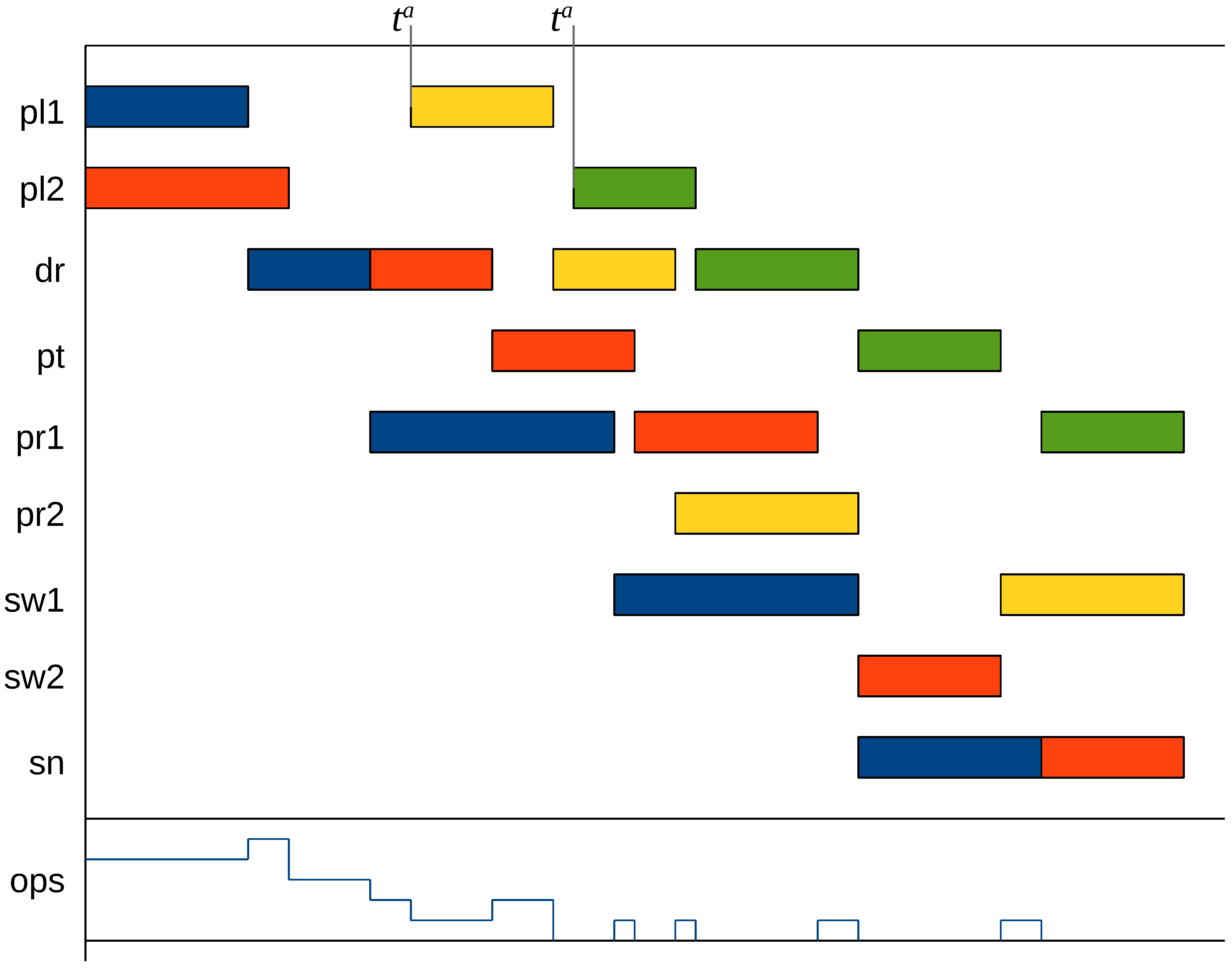
Figure 4 shows a schedule and how the timing of the operations is constrained by machine and operator availability, arrival times of shipments (indirectly through raw material availability), and the production order of the steps.

3. Proposed MILP Models

The models proposed in this section are based on the Start/End Event-based (SEE) and On/Off Event-based (OOE) models by Chakrabortty et al. [48]. These models were selected because they are among the best MILP models for MRCPSP in the literature, and their flexibility for extension. The models were adapted to solve the problem defined in Section 2, by adding new constraints and changing the objective function. In the following subsections, three variants are detailed, which address various issues differently. In Section 5 all variants are tested for efficiency and the most advantageous in practice is identified.

This section is structured as follows. Section 3.1 introduces variables, helper sets, constraints, and the objective, which is shared across all models. The SEE and OOE models are detailed in Section 3.2 and Section 3.3, respectively. The new notations of these 3 subsections are collected in

Table 4. Nomenclature for the MILP models.

Derived sets
$\mathcal{E}$	set of event points
$\Omega$	set of ordered pairs of orders from the same client
${\rho }_{a,v}$	lower bound on the cumulative usage of non-renewable resource $v\in V$ until activity $a\in A$ [$m^3$]
${\rho }_{s,v}^a$	the amount of non-renewable $v\in V$ shipped by the arrival time of shipment $s\in S$ [$m^3$]
$E{S}_a$	earliest starting time of $a\in A$ [h]
$L{S}_a$	latest starting time of $a\in A$ [h]
H	the length of the time horizon [h]
Variables
${\alpha }_{s,e}$	$\in \{0,1\}$ 1 if shipment $s\in S$ has arrived by the time of event $e\in \mathcal{E}$ [−]
${\delta }_o$	$\in \{0,1\}$ 0 if order $o\in O$ is canceled, 1 otherwise [−]
${\omega }_{o,o^{\prime }}$	$\in \{0,1\}$ 1 if the deadline of order o is changed to that of $o^{\prime }$ [−]
${\rho }_{e,r}^u$	$\in {\mathbb{R}}_0^{+}$ is the quantity of resource $r\in R$ in use at event $e\in \mathcal{E}$ [$m^3$]
${\tau }_o^d$	$\in {\mathbb{R}}_0^{+}$ the altered deadline of order $o\in O$ [h]
${\tau }_e$	$\in \left[0,H\right]$ the timing of event $e\in \mathcal{E}$ [h]
$x_{a,m,e}$	$\in \{0,1\}$ 1 if activity a starts in mode m at event e [−]
$y_{a,m,e}$	$\in \{0,1\}$ 1 if activity a ends in mode m at event e [−]
$z_{a,m,e}$	$\in \{0,1\}$ 1 if activity a is active in mode m at event e [−]

. Finally, Section 3.4 provides a coherent summary of the different variants.

3.1. Shared Features

The variables, constraints and the objective, which are related to the market environment, are shared across all models.

Binary variable ${\delta }_o$ is defined for all $o\in O$ and indicates whether o is fulfilled or canceled.

Deadlines of orders from the same client may be swapped. A derived set $\Omega$ contains all the possible ordered pairs of orders that share the same client:

$$\Omega :=\left\{(o,o^{\prime })\mid c_o=c_{o^{\prime }}\wedge o\ne o^{\prime }\right\}$$

Binary variable ${\omega }_{o,o^{\prime }}$ is defined for all of these pairs and indicates whether the deadline of o is changed to the deadline of $o^{\prime }$.

Based on these binary variables, the objective, i.e., the total penalty cost can be expressed:

$$\sum _{o\in O}{p}_o^c·(1-{\delta }_o)+\sum _{(o,o^{\prime })\in \Omega }{p}_{o,o^{\prime }}^s·{\omega }_{o,o^{\prime }}\to min$$

(1)

The changes of deadlines among orders must form a permutation, which is expressed by the following constraints. First, the deadline of an order may be changed to the deadline of at most one other order:

$$\sum _{(o,o^{\prime })\in \Omega }{\omega }_{o,o^{\prime }}\le 1\forall o\in O$$

(2)

Ensuring that the deadline of an order with a changed deadline gets assigned to another order is done by Equation (3):

$$\sum _{(o^{\ast },o)\in \Omega }{\omega }_{o^{\ast },o}=\sum _{(o,o^{\prime })\in \Omega }{\omega }_{o,o^{\prime }}\forall o\in O$$

(3)

While Equations (2) and (3) are sufficient constraints for setting the values of the swap decision variables $\omega$, Equation (4) is added to tighten the LP relaxation. It states that the deadline of an order o can only be reassigned to up to one other order:

$$\sum _{(o^{\ast },o)\in \Omega }{\omega }_{o^{\ast },o}\le 1\forall o\in O$$

(4)

Later timing constraints must use the new deadline of an order, instead of its original one, $t_o^d$. For this purpose, a non-negative calculated/derived variable is introduced to simplify modeling, ${\tau }_o^d$, which denotes the changed deadline. The proper relation between the parameter and this variable is expressed in Equation (5).

$${\tau }_o^d=t_o^d+\sum _{(o,o^{\prime })\in \Omega }\left(t_{o^{\prime }}^d-t_o^d\right)·{\omega }_{o,o^{\prime }}\forall o\in O$$

(5)

While technically it is allowed to swap the deadlines of two orders, and then cancel both, it results in a suboptimal solution; thus, Equation (6) is introduced to reduce the search space. It forbids swapping the deadlines of the orders o and $o^{\prime }$ if both of them are canceled.

$${\omega }_{o,o^{\prime }}\le {\delta }_o+{\delta }_{o^{\prime }}\forall (o,o^{\prime })\in \Omega$$

(6)

Moreover, it is easy to see that the deadline of a canceled order should not be changed to a later one. A better or equally good solution always exists where this order is removed from the permutation of deadlines. These redundant solutions are excluded from the search space by Equation (7). It forbids swapping the deadline of an order o with any later deadline $t_o^d$, if o is canceled.

$$\sum _{\begin{array}{c}(o,o^{\prime })\in \Omega \\ t_{o^{\prime }}^d\ge t_o^d\end{array}}{\omega }_{o,o^{\prime }}\le {\delta }_o\forall o\in O$$

(7)

Equations (4), (6) and (7) are aimed at improving solution performance by tightening the relaxation and reducing the search space by eliminating suboptimal or redundant solutions. These additional constraints may help to decrease solution time for some instances but it may increase computational burden in other cases. In our preliminary tests, using these constraints resulted in a 25% reduction in average solution time, so we kept them in the formulation.

The earliest and latest start times are often calculated from the project graph to provide bounds for the timing-related variables. Because of the deadlines and raw material deliveries, the definition of these bounds had to be altered slightly from those in [48].

The earliest start time may be delayed not only by prerequisite activities but by the arrival times of the required non-renewable resources.

First, the lower bound on the cumulative non-renewable resource usage up to activity a, denoted by ${\rho }_{a,v}$, is calculated based on the usages of preceding activities and minimum usage of the activity among its operation modes:

$${\rho }_{a,v}:=\underset{(a^{\ast },a)\in \Omega }{max}{\rho }_{a^{\ast },v}+\underset{m\in M_a}{min}{u}_{a,m,v}$$

Also, the amount of non-renewable $v\in V$ shipped cumulatively by the arrival of the shipment $s\in S$ is denoted by ${\rho }_{s,v}^a$, and can be calculated by summing up the material quantity of the shipment and all earlier shipments ($s^{\ast }\le s$):

$${\rho }_{s,v}^a:=\sum _{\begin{array}{c}{s}^{\ast }\in S_n\\ s^{\ast }\le s\end{array}}{q}_{s^{\ast }}^w$$

Using these parameters, the earliest and latest starting times of each activity, denoted by $E{S}_a$ and $L{S}_a$, can be calculated. The earliest starting time is lower bounded by the minimum durations of preceding activities, and the shipment time of all non-renewable resources required for the activity and its predecessors:

$$E{S}_a:=max\left\{0,\underset{(a^{\ast },a)\in P}{max}\underset{m\in M_{a^{\ast }}}{min}\left(E{S}_{a^{\ast }}+t_{a^{\ast },m}^p\right),\underset{v\in V}{max}\underset{\begin{array}{c}s\in S\\ {\rho }_{s,v}^a\ge {\rho }_{a,v}\end{array}}{min}{t}_s^a\right\}$$

The latest starting time is upper bounded by the latest deadline of an order from the same client, minus the remaining processing times:

$$L{S}_a:=\{\begin{array}{cc}\hfill \underset{o^{\prime }\in O,c_o=c_{o^{\prime }}}{max}{t}_{o^{\prime }}^d-\underset{m\in M_a}{min}{t}_{a,m}^p& \mathrm{i}\mathrm{f} a=a_o^l \mathrm{f}\mathrm{o}\mathrm{r} \mathrm{s}\mathrm{o}\mathrm{m}\mathrm{e} o\in O,\\ \hfill \underset{(a,a^{\prime })\in P}{max}L{S}_{a^{\prime }}-\underset{m\in M_a}{min}{t}_{a,m}^p& \mathrm{o}\mathrm{t}\mathrm{h}\mathrm{e}\mathrm{r}\mathrm{w}\mathrm{i}\mathrm{s}\mathrm{e}\end{array}$$

Both types of models rely on a set of events, which will be denoted by $\mathcal{E}=\{1,2,\dots ,|\mathcal{E}\left|\right\}$. The events are points in time where activities may start or end. The number of events can be set to $\left|A\right|+\left|O\right|$ to guarantee optimality ($\left|A\right|+2·\left|O\right|$ for the SEE model), or set to a lower number to decrease solution time. There is no known formula for the minimum necessary number of events to find the optimal solution. This issue is discussed in more detail in Section 5.1.

The time when an event $e\in \mathcal{E}$ occurs is set by the continuous variable ${\tau }_e\in \left[0,H\right]$. H denotes the time horizon length, which is equal to the latest deadline: $H:={max}_{o\in O}{t}_o^d$. To reduce redundancy, Equation (8) constrains the event times to be non-decreasing.

$${\tau }_{e-1}\le {\tau }_e\forall e\in \mathcal{E},e>1$$

(8)

Equations (9) and (10) calculate whether the materials of a shipment $s\in S$ have arrived and are available at event $e\in \mathcal{E}$. The binary variable ${\alpha }_{s,e}$ is 1 if the s has arrived by the time of event e.

$${\tau }_e\ge t_s^a·{\alpha }_{s,e}\forall s\in S,e\in \mathcal{E}$$

(9)

$${\tau }_e\le t_s^a+H·{\alpha }_{s,e}\forall s\in S,e\in \mathcal{E}$$

(10)

As the events and shipments are ordered by their timing, it follows that if a shipment has arrived by event $e-1$, it must also be available at event e (Equation (11)), and all earlier shipments must have arrived by that event too (Equation (12)). These tightening constraints can improve solution performance.

$${\alpha }_{s,e-1}\le {\alpha }_{s,e}\forall s\in S,e\in \mathcal{E},e>1$$

(11)

$${\alpha }_{s^{\prime },e}\le {\alpha }_{s,e}\forall s,s^{\prime }\in S,s<s^{\prime },e\in \mathcal{E}$$

(12)

Equation (13) is also added because the first stage of each order requires shipped non-renewable resources in the investigated problem. Initial resource stock can be represented by a shipment arriving at time 0.

$$\sum _{s\in S}{\alpha }_{s,e}\ge 1\forall e\in \mathcal{E}$$

(13)

3.2. Start/End Event-Based Model (SEE)

The titular binary assignment variables of the SEE model are $x_{a,m,e}$ and $y_{a,m,e}$, denoting whether activity a starts or ends in operation mode m at event e.

In the model by Chakrabortty et al. [48], each activity is started and ended in exactly 1 mode at 1 event. However, since orders may be canceled in the current problem, the right sides of Equations (14) and (15) contain ${\delta }_o$ instead of 1.

$$\sum _{m\in M_a}\sum _{e\in \mathcal{E}}{x}_{a,m,e}={\delta }_{o_a}\forall a\in A$$

(14)

$$\sum _{m\in M_a}\sum _{e\in \mathcal{E}}{y}_{a,m,e}={\delta }_{o_a}\forall a\in A$$

(15)

Although it is missing from the proposed formulation in [48], Equation (16) is necessary to ensure that each activity is ended in the same mode it was started in.

$$\sum _{e\in \mathcal{E}}{x}_{a,m,e}=\sum _{e\in \mathcal{E}}{y}_{a,m,e}\forall a\in A,m\in M_a$$

(16)

The lower bound on the time difference between the start and end of an activity is set to the processing time by Equation (17).

$${\tau }_{e^{\prime }}\ge {\tau }_e+t_{a,m}^p·\left(x_{a,m,e}+y_{a,m,e^{\prime }}-1\right)\forall a\in A,m\in M_a,e,e^{\prime }\in \mathcal{E},e<e^{\prime }$$

(17)

As Equation (17) is only defined for $e<e^{\prime }$, it would allow an activity to end before it has started. To correct this, the constraints defined in [48] are extended with Equation (18), and its inverse, Equation (19), is added for better solution performance.

$$\sum _{m\in M_a}{x}_{a,m,e}\le 1-\sum _{m\in M_a}\sum _{\begin{array}{c}{e}^{\ast }\in \mathcal{E}\\ e^{\ast }\le e\end{array}}{y}_{a,m,e^{\ast }}\forall a\in A,e\in \mathcal{E}$$

(18)

$$\sum _{m\in M_a}{y}_{a,m,e}\le 1-\sum _{m\in M_a}\sum _{\begin{array}{c}{e}^{\prime }\in \mathcal{E}\\ e\le e^{\prime }\end{array}}{x}_{a,m,e^{\prime }}\forall a\in A,e\in \mathcal{E}$$

(19)

Precedence relations are set by Equation (20).

$$\sum _{m\in M_{a^{\prime }}}\sum _{\begin{array}{c}{e}^{\ast }\in \mathcal{E}\\ e^{\ast }<e\end{array}}{x}_{a^{\prime },m,e^{\ast }}\le 1-\sum _{m\in M_a}\sum _{\begin{array}{c}{e}^{\prime }\in \mathcal{E}\\ e\le e^{\prime }\end{array}}{y}_{a,m,e^{\prime }}\forall (a,a^{\prime })\in P,e\in \mathcal{E},e>1$$

(20)

To model order deadlines, a new constraint, Equation (21) is defined. It constrains the timing of an event associated with the finish of an activity to be earlier than the deadline of the order containing that activity.

$${\tau }_e\le {\tau }_o^d+H·\left(1-\sum _{m\in M_{a_o^l}}{y}_{a_o^l,m,e}\right)\forall o\in O,e\in \mathcal{E}$$

(21)

The $E{S}_a$ and $L{S}_a$ values are used in Equations (22)–(24) to improve solution performance. They are similar to the ones in [48] but summation over $m\in M_a$ is used where possible instead of defining a separate inequality for each $(a,m)$ pair, as this formulation achieves even better performance.

$$E{S}_a·\sum _{m\in M_a}{x}_{a,m,e}\le {\tau }_e\le L{S}_a+H·\left(1-\sum _{m\in M_a}{x}_{a,m,e}\right)\forall a\in A,e\in \mathcal{E}$$

(22)

$${\tau }_e\ge \sum _{m\in M_a}\left(E{S}_a+t_{a,m}^p\right)·y_{a,m,e}\forall a\in A,e\in \mathcal{E}$$

(23)

$${\tau }_e\le L{S}_a+t_{a,m}^p+H·(1-y_{a,m,e})\forall a\in A,m\in M_a,e\in \mathcal{E}$$

(24)

The constraints for renewable resources are the same as in [48]. The quantity of resource $r\in R$ in use at event e is set by the nonnegative variable ${\rho }_{e,r}^u$, whose upper bound is the resource capacity, set by Equation (25). Its value is calculated in Equation (26) for the first event, and Equation (27) for subsequent events.

$${\rho }_{e,r}^u\le q_r^c\forall e\in \mathcal{E},r\in R$$

(25)

$${\rho }_{1,r}^u=\sum _{a\in A,m\in M_a}{u}_{a,m,r}·x_{a,m,1}\forall r\in R$$

(26)

$${\rho }_{e,r}^u={\rho }_{e-1,r}^u+\sum _{a\in A}\sum _{m\in M_a}{u}_{a,m,r}·(x_{a,m,e}-y_{a,m,e})\forall e\in \mathcal{E},e>1,r\in R$$

(27)

The non-renewable resource constraint needed modification to handle raw material shipments. Equation (28) calculates the quantities consumed up to and available at each event point, for every resource, and ensures their balance.

$$\sum _{a\in A}\sum _{m\in M_a}\sum _{\begin{array}{c}{e}^{\ast }\in \mathcal{E}\\ e\ast \le e\end{array}}{u}_{a,m,v}·x_{a,m,e^{\ast }}\le \sum _{s\in S_v}{q}_s^w·{\alpha }_{s,e}\forall e\in \mathcal{E},v\in V$$

(28)

3.3. On/Off Event-Based Model (OOE)

As its name suggests, in the OOE model the binary decision variables ($z_{a,m,e}$) denote whether an activity is active (being processed) at an event point. For a simpler formulation, the variable is also defined for $e=0$, and $z_{a,m,0}=0$ for all $a\in A,m\in M_a$.

Equation (29) states that every activity of an accepted order is active at least once. Since there is no use for execution activities of refused orders, Equation (30) is added to improve the model.

$$\sum _{m\in M_a}\sum _{e\in \mathcal{E}}{z}_{a,m,e}\ge {\delta }_{o_a}\forall a\in A$$

(29)

$$\sum _{m\in M_a}{z}_{a,m,e}\le {\delta }_{o_a}\forall a\in A,e\in \mathcal{E}$$

(30)

Precedence relations are enforced by Equation (31).

$$\sum _{\begin{array}{c}{e}^{\ast }\in \mathcal{E}\\ e^{\ast }\le e\end{array}}\sum _{m\in M_{a^{\prime }}}{z}_{a^{\prime },m,e^{\ast }}\le e·\left(1-\sum _{m\in M_a}{z}_{a,m,e}\right)\forall (a,a^{\prime })\in P,e\in \mathcal{E}$$

(31)

The advantage of using on/off variables instead of start/stop variables, aside from having half as many binary variables, is that modeling renewable resource constraints is easier, as shown by Equation (32). There is no need to define continuous variables for calculating resource usage at an event point.

$$\sum _{a\in A}\sum _{m\in M_a}{u}_{a,m,r}·z_{a,m,e}\le q_r^c\forall e\in \mathcal{E},r\in R$$

(32)

Modeling non-renewable resource constraints, however, is more difficult because an activity can be active over several event points, so multiplying $z_{a,m,e}$ with the resource usage is not a good solution. The OOE model by Chakrabortty et al. [48] does not contain constraints for modeling non-renewable resource capacities. With a mode assignment variable, indexed by activity and mode, it is possible to calculate the total resource usage to solve the original MRCPSP with non-renewable resources. However, in the problem at hand because of material shipments, the total resource usage is not enough but the time of usage is important too. Therefore, the variable needs to be indexed not only by the activity and mode but also by the event when the resources are consumed. This is equivalent to the start variable of the SEE model, $x_{a,m,e}$. So x is added to the OOE model and connected to the z variables by Equation (33). The expression $z_{a,m,e}-z_{a,m,e-1}$ is used in several constraints in [48], so they are replaced by x where possible for better clarity and performance.

$$x_{a,m,e}\ge z_{a,m,e}-z_{a,m,e-1}\forall a\in A,m\in M_a,e\in \mathcal{E}$$

(33)

From the SEE model Equation (14) is added to this extended OOE model to tighten the formulation, and Equation (28) is added as the non-renewable resource constraint.

Based on processing times, Equation (34) sets a lower bound on future events where an activity that started in the past is not active anymore.

$${\tau }_{e^{\prime }}\ge {\tau }_e+\sum _{m\in M_a}{t}_{a,m}^p·(x_{a,m,e}-z_{a,m,e^{\prime }})\forall a\in A,e,e^{\prime }\in \mathcal{E},e<e^{\prime }$$

(34)

Equations (35) and (36) are contiguity constraints to ensure that each activity is active over a single contiguous sequence of event points from its start to its end.

$$\sum _{\begin{array}{c}{e}^{\ast }\in \mathcal{E}\\ e^{\ast }<e\end{array}}{z}_{a,m,e^{\ast }}\le e·\left(1-\sum _{m\in M_a}{x}_{a,m,e}\right)\forall a\in A,e\in \mathcal{E}$$

(35)

$$\sum _{\begin{array}{c}{e}^{\prime }\in \mathcal{E}\\ e<e^{\prime }\end{array}}{z}_{a,m,e^{\prime }}\le \left(\left|\mathcal{E}\right|-e\right)·\left(1+\sum _{m\in M_a}\left(z_{a,m,e}-z_{a,m,e-1}\right)\right)\forall a\in A,e\in \mathcal{E}$$

(36)

The earliest and latest start times of the activities are used in Equations (37) and (38) to increase solution performance.

$${\tau }_e\ge E{S}_a·z_{a,m,e}\forall a\in A,m\in M_a,e\in \mathcal{E}$$

(37)

$${\tau }_e\le L{S}_a+H·\left(1-\sum _{m\in M_a}{x}_{a,m,e}\right)\forall a\in A,e\in \mathcal{E}$$

(38)

The deadline constraint can be defined in multiple ways. Equation (39) calculates the end time of an activity from its starting and processing time, and bounds it by the deadline. While Equation (39) would be enough on its own, performance can be improved by also connecting z variables with the deadlines, as done by Equation (40). To combine these two inequalities, Equation (41) is defined to be used in the OOE2 model variant.

$${\tau }_e+t_{a,m}^p\le {\tau }_{o_a}^d+H·\left(1-x_{a,m,e}\right)\forall a\in A,m\in M_a,e\in \mathcal{E}$$

(39)

$${\tau }_{e+1}\le {\tau }_{o_a}^d+H·\left(1-\sum _{m\in M_a}{z}_{a,m,e}\right)\forall a\in A,e\in \mathcal{E},e<\left|\mathcal{E}\right|$$

(40)

$${\tau }_e+\sum _{m\in M_a}{x}_{a,m,e}·t_{a,m}^p\le {\tau }_{o_a}^d+H·\left(1-\sum _{m\in M_a}{z}_{a,m,e}\right)\forall a\in A,e\in \mathcal{E}$$

(41)

3.4. Summary of Variants

Three model variants have been selected for further empirical analysis: one SEE model, and two variants of the OOE model. The SEE model consists of Equations (1)–(28). The OOE1 model is made up of Equations (1)–(14) and Equations (28)–(40). The OOE2 model is defined by Equations (1)–(14), Equations (28)–(38), and Equation (41).

The redundant constraints of the above variants have shown considerable performance improvements in preliminary tests. Other potentially strengthening constraints have been tested as well but showed no significant effect, or led to higher solution times. It is possible that these constraints prove to be more useful for problems with different characteristics, or when using different optimization software. For this reason, the rejected constraints are presented below.

Equation (18) can be formulated tighter by changing the 1 on the right side to ${\delta }_{o_a}$, as shown in Equation (42). If ${\delta }_{o_a}=0$ then $x_{a,m,e}=0$ as well, for any m and e. However, using a constant instead of a variable worked better.

$$\sum _{m\in M_a}{x}_{a,m,e}\le {\delta }_{o_a}-\sum _{m\in M_a}\sum _{\begin{array}{c}{e}^{\ast }\in \mathcal{E}\\ e^{\ast }\le e\end{array}}{y}_{a,m,e^{\ast }}\forall a\in A,e\in \mathcal{E}$$

(42)

Equation (21) can also be tightened by summing over all future events, not just the current event, to see if the order is finished there. The current event, e, must happen before the deadline of the order in both cases. However, the variant in Equation (43) did not perform better overall.

$${\tau }_e\le {\tau }_o^d+H·\left(1-\sum _{m\in M_{a_o^l}}\sum _{\begin{array}{c}{e}^{\prime }\in \mathcal{E}\\ e\le e^{\prime }\end{array}}{y}_{a_o^l,m,e}\right)\forall o\in O,e\in \mathcal{E}$$

(43)

As seen in Equation (36), the OOE formulation does not have dedicated variables for when an activity ends. With this method, a bound on the earliest and latest finish of an activity can be defined, not just on the earliest and latest start, as shown in Equations (44) and (45).

$${\tau }_e\ge \sum _{m\in M_a}\left(E{S}_a+t_{a,m}^p\right)·\left(z_{a,m,e-1}-z_{a,m,e}\right)\forall a\in A,e\in \mathcal{E}$$

(44)

$${\tau }_e\le L{S}_a+t_{a,m}^p+H·\left(1+z_{a,m,e}-z_{m,e-1}\right)\forall a\in A,m\in M_a,e\in \mathcal{E}$$

(45)

A substantial amount of redundancy is present by having more event points than necessary. Many equivalent solutions are permitted by the model, differing only in what event points are used or unused. Naturally, the best would be not to use more event points than needed but it is difficult to determine the required number. This issue is discussed in Section 5.1. However, this redundancy can be decreased with constraints as well. To constrain all unused events to go after the used events, Equation (46) can be added to the SEE model, or Equation (47) to the OOE model.

$$\sum _{a\in A}\sum _{m\in M_a}\sum _{\begin{array}{c}{e}^{\prime }\in \mathcal{E}\\ e<e^{\prime }\end{array}}\left(x_{a,m,e^{\prime }}+y_{a,m,e^{\prime }}\right)\le \left|A\right|·\sum _{a\in A}\sum _{m\in M_a}\left(x_{a,m,e}+y_{a,m,e}\right)\forall e\in \mathcal{E}$$

(46)

$$\sum _{a\in A}\sum _{m\in M_a}\sum _{\begin{array}{c}{e}^{\prime }\in \mathcal{E}\\ e<e^{\prime }\end{array}}{z}_{a,m,e^{\prime }}\le \left|A\right|·\sum _{a\in A}\sum _{m\in M_a}{z}_{a,m,e}\forall e\in \mathcal{E}$$

(47)

Scalability Analysis

The shared swap and shipment structure introduces $|\Omega |+\left|O\right|$ binary variables, where $|\Omega |$ is 0 in the best case and ${\displaystyle \frac{\left(\right|O|-1)\left|O\right|}{2}}$ in the worst case. All model variants use an additional $2\left|\mathcal{E}\right|{\sum }_{a\in A}\left|M_a\right|$ binary variables for the scheduling decisions. While this formula cannot be simplified in a general case, if $O=O^P$, $|E_k|=m$ for all $k\in K$, and we use $\left|\mathcal{E}\right|=\left|A\right|+\left|O\right|$ time points, then each model variant introduces $2\left(\right|A|+\left|O\right|\left)\right|O\left|\right|K|2^m=\left(\right|K|+{1\left)\right|K\left|\right|O|}^2{2}^{m+1}$ binary variables. $\left|K\right|$ is constant and for practical applications, $\left|C\right|$ can be considered constant for a single facility, as well as the $|E_k|$ values. As a result, extending the considered time horizon, and thus increasing $\left|O\right|$ and $\left|\mathcal{E}\right|$ would have a quadratic effect on the number of swap binary variables.

While the exact number of constraints for each model is a convoluted expression, it is worth highlighting that Equation (17) and Equation (34) introduce ${\sum }_{a\in A}\left|M_a\right|{\displaystyle \frac{\left(\right|\mathcal{E}|-1)\left|\mathcal{E}\right|}{2}}$ and $\left|A\right|{\displaystyle \frac{\left(\right|\mathcal{E}|-1)\left|\mathcal{E}\right|}{2}}$ constraints, respectively. Both are quadratic in $\left|\mathcal{E}\right|$ and thus cubic in $\left|O\right|$.

As a conclusion, the number of orders, and thus the number of time points is the key scalability driver.

4. Proposed GA Approach

As the early tests have shown, the MILP models are only suitable for small instances. Solving real-world scenarios to optimality would take too much computational time for practical application. Hence, we developed a metaheuristic approach based on the Genetic Algorithm (GA) methodology to solve larger instances. Initial results of this approach were briefly presented in [57]. Since then, we further developed the algorithm with an improved cost calculation procedure and new crossover methods, and optimized the hyperparameters based on empirical analysis. This section presents the improved version of the GA solution method.

4.1. The GA Framework

The proposed GA approach was developed using the openGA C++ library [58], which provides the high-level optimization algorithm. The solution representation, cost function, and genetic operators were implemented for the investigated problem. These are detailed in the following subsections.

The solution procedure starts with a randomly generated initial population of solutions. The population size hyperparameter sets the number of solutions, which is constant throughout the generations. The algorithm then iterates through the following steps until one of the termination conditions is met:

• Crossover: Pairs of solutions are selected (with better solutions having higher probability) and recombined to create new solutions.
• Mutation: Some of the new solutions are mutated to introduce new information.
• Selection: Solutions are selected for the next generation with probabilities based on solution quality. If the $elite\_count$ parameter is set, then the best $elite\_count$ solutions are selected automatically.

The algorithm terminates when the maximum number of generations is reached, or when the solutions have not improved for a given number of generations. The latter is split into two conditions with separate threshold parameters: if the best solution has not improved, or if the average solution has not improved.

4.2. Solution Representation

The genes of an individual are stored as an array of double-precision floating-point numbers, with one number for each activity ($g_a\forall a\in A$). These numbers encode 3 decisions for each activity:

• Operation mode assignment;
• Order cancellation;
• Priority value.

The integral part of a gene value ($\lfloor g_a\rfloor$) determines the index of the operation mode assigned to the activity, so it is ensured that $0\le g_a<\left|M_a\right|-1$. In the initial population, the values are randomly generated in this range with uniform distribution.

The fractional part of the gene value determines the priority of the activity within the encoded schedule (lower values mean earlier start times). As there are fixed precedence relations between the activities related to a single order, the priorities of predecessors need to be adjusted accordingly:

$$prio\left(a\right)=\left\{\begin{array}{cc}frac\left(g_a\right)\hfill & \mathrm{i}\mathrm{f} a=a_{o_a}^l\hfill \\ min\left(frac\left(g_a\right),\underset{(a,a^{\prime })\in P}{min}prio\left(a^{\prime }\right)\right)\hfill & \mathrm{o}\mathrm{t}\mathrm{h}\mathrm{e}\mathrm{r}\mathrm{w}\mathrm{i}\mathrm{s}\mathrm{e}\hfill \end{array}\right.$$

The least significant 24 bits of the value are also used to decide if the order associated with the activity should be canceled. If the value of these bits is in the lower 5% of the possible values, the order is canceled: $canceled\left(a\right)\iff g_a\otimes (2^{24}-1)\le 0.05·2^{24}$.

The priority values of the final activities of the orders are also used to determine deadline swaps. For each client, the order deadlines are reassigned in priority order, possibly resulting in swaps. The pseudocode of this procedure is shown in Algorithm 1.

Algorithm 1 Reassign order deadlines and calculate swap costs.

1: function make_deadline_swaps(g) 2:     $swap\_cost\leftarrow 0$ 3:     $new\_deadlines\leftarrow [t_o^d\mid o\in O]$ 4:     for all $c\in C$ do                                                                                                                                     ▹ Handle each client separately 5:         $order{s}_c\leftarrow [o\mid o\in O_c]$ 6:         $order{s}_c^t\leftarrow$sorted($order{s}_c,key:o\mapsto t_o^d$)                                                                                                 ▹ Orders sorted chronologically 7:         $order{s}_c^p\leftarrow$sorted($order{s}_c,key:o\mapsto prio\left(a_o^l\right)$)                                                                                              ▹ Orders sorted by priority 8:         for $i\leftarrow 1,\dots ,|order{s}_c|$ do 9:            $new\_deadlines\left[order{s}_c^p\left[i\right]\right]\leftarrow t_{order{s}_c^t\left[i\right]}^d$ 10:            if $t_{order{s}_c^p\left[i\right]}^d\ne t_{order{s}_c^t\left[i\right]}^d$ then 11:                $swap\_cost\leftarrow swap\_cost+p_{order{s}_c^p\left[i\right],order{s}_c^t\left[i\right]}^s$ 12:            end if 13:         end for 14:     end for 15:     return $swap\_cost,new\_deadlines$ 16: end function

4.3. Solution Decoding and Cost Calculation

Start times are not encoded in the gene representation; they are determined during the decoding process. The complete schedule and the costs associated with it are calculated by Algorithm 2. This procedure iterates over the activities in priority order, and schedules them one by one as early as possible, delaying start times when necessary to satisfy resource constraints. If an order exceeds its deadline, it is canceled, and the procedure is restarted. This way, each solution is decoded to a feasible schedule where all orders are either canceled or finished on time.

Algorithm 2 Scheduling and cost calculation.
1: function total_costs(g)
2:    swapcosts, deadlines ← make_deadline_swaps(g)
3:    $latest\_finish\leftarrow \left[LF\right(a,deadlines)\mid a\in A]$
4:    $accepted\leftarrow \{o\mid o\in O,\nexists a\in A:o_a=o\wedge canceled\left(a\right)\}$
5:    $sortedA\leftarrow [a\mid a\in A,o_a\in accepted]$
6:    sort($sortedA,key:a\mapsto prio\left(a\right)$)
7:    $\tau \leftarrow [0\mid a\in sortedA]$	▹ Activity start times
8:    ${\tau }^m\leftarrow [0\mid e\in E]$	▹ Machine finish times
9:    ${\rho }^m\leftarrow q^m$	▹ Available manual operators
10:    ${\rho }^w\leftarrow [0\mid w\in W]$	▹ Stock levels
11:    for all $w\in W$ do
12:        ${\alpha }_w\leftarrow [(t_s^a,q_s^w)\mid s\in S_w]$	▹ Queue of incoming shipments
13:    end for
14:    ${\alpha }^m\leftarrow \left[\right]$	▹ Queue of returning manual operators
15:    for $i\leftarrow 1,\dots ,\left|sortedA\right|$ do
16:        $a\leftarrow sortedA\left[i\right]$
17:        for all $e\in E_{a,\lfloor g_a\rfloor }$ do	▹ Wait until the required units become available
18:           $\tau \left[a\right]\leftarrow max\left(\tau \left[a\right],{\tau }^m\left[e\right]\right)$
19:        end for
20:        if $i>1$ then	▹ Cannot start before higher priority activity
21:           $\tau \left[a\right]\leftarrow max\left(\tau \left[a\right],\tau \left[sortedA\right[i-1\left]\right]\right)$
22:        end if
23:        for all $(a^{\prime },a)\in P$ do	▹ Cannot start before all predecessors are finished
24:           $\tau \left[a\right]\leftarrow max\left(\tau \left[a\right],\tau \left[a^{\prime }\right]+t_{a^{\prime },\lfloor g_{a^{\prime }}\rfloor }^p\right)$
25:        end for
26:        if $\nexists (a^{\prime },a)\in P$ then	▹ First step cannot start until enough wood is available
27:           while $q_{o_a}^r>{\rho }^w\left[w_{o_a}\right]$ do
28:               if ${\alpha }_{w_{o_a}}=\varnothing$ then
29:                   $g\left[a\right]\leftarrow 0$	▹ Cancel the order and restart
30:                   return total_costs(g)
31:               end if
32:               $(arrival,qty)\leftarrow$ pop_first $\left({\alpha }_{w_{o_a}}\right)$
33:               $\tau \left[a\right]\leftarrow max\left(\tau \left[a\right],arrival\right)$
34:               ${\rho }^w\left[w_{o_a}\right]\leftarrow {\rho }^w\left[w_{o_a}\right]+qty$
35:           end while
36:           ${\rho }^w\left[w_{o_a}\right]\leftarrow {\rho }^w\left[w_{o_a}\right]-q_{o_a}^r$
37:        end if
38:        $op\_needed\leftarrow {\displaystyle \sum _{e\in E_{a,\lfloor g_a\rfloor }}}{q}_e^m$
39:        while $op\_needed>{\rho }^m$ do	▹ Cannot start before enough operators are available
40:           $(arrival,qty)\leftarrow$ pop_first $\left({\alpha }^m\right)$
41:           $\tau \left[a\right]\leftarrow max\left(\tau \left[a\right],arrival\right)$
42:           ${\rho }^m\leftarrow {\rho }^m+qty$
43:        end while
44:        ${\rho }^m\leftarrow {\rho }^m-op\_needed$
45:        if $\tau \left[a\right]+t_{a,\lfloor g_a\rfloor }^p>latest\_finish\left[a\right]$ then	▹ The order deadline cannot be met
46:           $g\left[a\right]\leftarrow 0$	▹ Cancel the order and restart
47:           return total_costs(g)
48:        end if
49:        $finish\_time\leftarrow \tau \left[a\right]+t_{a,\lfloor g_a\rfloor }^p$
50:        ${\tau }^m\left[e\right]\leftarrow finish\_time$
51:        ${\alpha }^m\leftarrow$ push_sorted $({\alpha }^m,(finish\_time,op\_needed))$
52:    end for
53:    return $swapcosts+{\displaystyle \sum _{o\in O\setminus accepted}}{p}_o^c$
54: end function

The decoding procedure deterministically constructs a single schedule from a genetic code. While this excludes some schedules from consideration, those only differ from the constructed schedule in the start times of the activities, which do not directly affect the objective value. The total costs only depend on (1) the costs of deadline swaps, which are determined by the genes through priority values, and (2) cancellation costs, which are partly determined by the gene values ($canceled\left(a\right)$), and partly during the decoding process when the resulting schedule would violate deadline constraints.

The decoding procedure does not exclude all optimal schedules. For every feasible schedule, there exists a genetic code, which is decoded to a schedule with an equal objective value. To construct such a genetic code, take the activity start times of the schedule in increasing order, assign increasing priority values (fractional values) to their activities respecting any necessary deadline swaps and the cancellation threshold, and set the mode assignments (integral values) based on the schedule.

Algorithm 2 constructs a schedule and calculates its costs in the following way. First, the deadline swaps are determined by Algorithm 1. Then the latest allowed finish times are calculated for each activity from the deadlines, as shown in Algorithm 3. Then the activities of accepted orders are sorted by priority, and their start times are decided one by one. The start time is set as early as possible while ensuring that the current activity:

• cannot start before the previously scheduled activity;
• cannot start before all required units are available;
• cannot start before all predecessors are finished;
• cannot start before enough wood is available;
• cannot start before enough manual operators are available.

Algorithm 3 Determine latest allowed finish time of an activity.

1: function LF($a,deadlines$) 2:     if $a=a_{o_a}^l$then                                                 ▹ Final activity of an order 3:         return $deadlines\left[o_a\right]$ 4:     else 5:         return $\underset{(a,a^{\prime })\in P}{max}\left(\mathrm{LF}(a^{\prime },deadlines)-\underset{m\in M_{a^{\prime }}}{min}{t}_{a^{\prime },m}^p\right)$ 6:     end if 7: end function

If the activity would finish later than its latest allowed finish time, its order is canceled and the algorithm is restarted.

4.4. Genetic Operators

The GA uses two genetic operators: crossover and mutation. For the crossover operator, 3 different methods were implemented and compared: one-point, two-point, and uniform.

In one-point crossover, a random point is selected in the gene array then the genes before are copied from one parent and the genes after are copied from the other parent. In two-point crossover, two random points are selected and one parent is used for the genes between the points, while the other parent is used for the outer genes. In uniform crossover, the parent is selected for each gene separately, with equal probability.

For mutation, the number of genes to be altered is determined by a random integer between 1 and 5. The genes are selected randomly, and their values are adjusted by a random number taken uniformly from $[-1,1]$. Then, if the value is outside the allowed range, it is increased or decreased by $|M_a|$ accordingly.

5. Empirical Evaluation

All of the model variants proposed in Section 3.4 have been extensively tested on randomly generated examples. The tests were carried out on a laptop with an Intel i7-13700H 5.0 GHz CPU and 32 GB RAM, using the Gurobi 12.0.3 solver for MILP models, and a C++ implementation of the GA, using the OpenGA library [58].

The number of event points, i.e., $\left|\mathcal{E}\right|$ has a huge impact on the performance of the MILP models; Section 5.1 discusses the selection strategy for this number. The test instances were generated based on data from a real-life case study of a Central European plywood production plant, as discussed in Section 5.2. The empirical analysis of the MILP model variants is discussed in Section 5.3. The hyperparameter tuning of the GA approach is shown in Section 5.4. Finally, Section 5.5 presents the performance comparison of the approaches.

5.1. The Number of Event Points

Time discretization-based scheduling models allow the system to change its behavior at specific points in time, which are often referred to as time points or event points. The maximal number of these event points is a configuration parameter of these models, which influences both the quality of the reported solution and the computational needs. Usually, computational time explodes exponentially while gradually increasing the number of available event points, as the number of binary variables is a linear function of that. Thus, it is a general desire to find the optimal solution with the lowest number of event points possible. Although there were some studies conducted [59], there is no exact formula to provide that number.

A widely used approach with such models is to iteratively solve the model with an increasing number of event points. This approach could be appropriate in practice with only a single instance to be solved; however, it is not suitable for comparing several model variants on a large number of instances with varying time limits. Thus, the considered number of event points needed to be fixed for our comparisons.

It is rather easy to provide reasonable lower and upper bounds on the number of event points. An order that does not require patching has 5 steps, which require at least 6 event points to be scheduled. In theory, this could suffice for the optimal solution in some cases, if all of the orders can be executed in parallel. Following a similar idea, if none of the activities share event points across orders, then $\left|A\right|+\left|O\right|$ event points would be needed.

In order to fix the number of the event points for the extensive testing detailed in Section 5.3, several preliminary tests were run following the aforementioned iterative strategy.

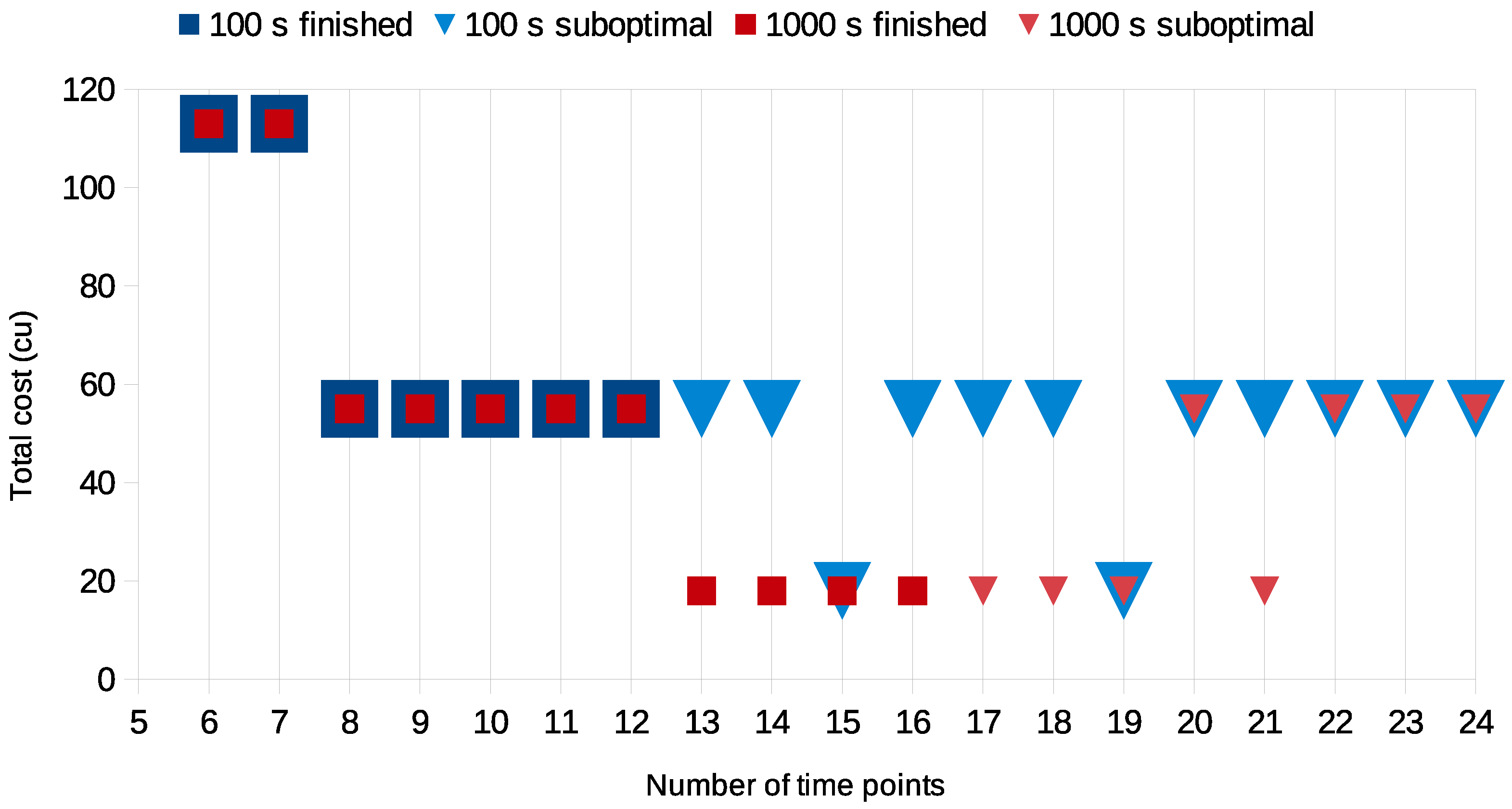
Figure 5 shows the results of one such test suite. The instance has two clients and 4 orders with deadlines in the range of 5 to 8 days (with 24 h workdays). Swapping costs are generated to be client-dependent, either 6 or 9 cost units (cu) for all order pairs of the same client, while cancellation cost ranges from 55 to 74 cu. None of the orders require patching, so the number of event points were increased from 6 to 24, and two different time limits were considered: 100 s and 1000 s with the model variant OOE2.

Figure 5 shows the best solution found for every number of event points. Blue colored indicators belong to the 100 s runs, while red ones to 1000 s runs. Square shapes indicate that optimality for the current number of event points was proved within the respective time limit, while the optimizer stopped at a suboptimal solution or could not prove the solution’s optimality in the case of downward-facing triangles with lighter colors.

Several conclusions can be drawn from this example. Understandably, increasing the time limit tenfold allowed the optimizer to finish and prove optimality for additional 4 instances with more event points. Overall, in all of the runs, only 3 different solutions were reported with respective values of 113, 55, and 18. The optimality of the 18 cu solution could only be proved within the 1000 s time limit for event points 13 to 17.

An interesting phenomenon occurred for both time limits: additional event points may result in worse solutions, as the optimizer has difficulty finding the optimal solution. While it is theoretically possible that a better solution than 18 cu is feasible with 24 event points, the 1000 s was not enough for the optimizer to even find the 18 cu solution. Thus, in a practical sense, allowing more event points did not only not provide better results, it actually worsened the reported solution. For both time limits, the results suggest a threshold value for the number of event points, which acts as a divider for proving optimality under the time limit. Having more event points beyond this threshold is actually disadvantageous.

Tests carried out on other examples showed similar results. Thus, as a compromise between proven optimality of $\left|A\right|+\left|O\right|$ event points, and the experienced lower values from the preliminary tests, $\left|\mathcal{E}\right|$ was set to $\left|A\right|$ for all of the following experiments, with 3600 s time limit.

5.2. Problem Generation

Instances were randomly generated for 8 scenarios, differing in the number of orders, clients, and the length of the time horizon, as shown in

Table 5. Main parameter values of the scenarios.

Dataset	# Orders	# Clients	Time Horizon [Days]	# Instances
7d3j1c	3	1	7	20
7d4j2c	4	2	7	20
10d3j1c	3	1	10	20
10d4j2c	4	2	10	20
30d10j4c	10	4	30	10
30d10j5c	10	5	30	10
30d12j5c	12	5	30	10
30d15j10c	15	10	30	10

. The 4 smaller (7 and 10 days long) scenarios contain 20 instances, and the 30-day scenarios contain 10 instances each.

The set of equipment units and their parameters are the same in all instances. There are 1–3 machines at each step; their throughput [${\mathrm{m}}^3$/h] and manual operator requirements are shown in

Table 6. Machine parameters.

Peeling		Drying		Patching		Pressing		Sawing		Sanding
${\mathit{f}}_{\mathit{e}}^{\mathit{w}}$	${\mathit{q}}_{\mathit{e}}^{\mathit{m}}$	${\mathit{f}}_{\mathit{e}}^{\mathit{w}}$	${\mathit{q}}_{\mathit{e}}^{\mathit{m}}$	${\mathit{f}}_{\mathit{e}}^{\mathit{w}}$	${\mathit{q}}_{\mathit{e}}^{\mathit{m}}$	${\mathit{f}}_{\mathit{e}}^{\mathit{w}}$	${\mathit{q}}_{\mathit{e}}^{\mathit{m}}$	${\mathit{f}}_{\mathit{e}}^{\mathit{w}}$	${\mathit{q}}_{\mathit{e}}^{\mathit{m}}$	${\mathit{f}}_{\mathit{e}}^{\mathit{w}}$	${\mathit{q}}_{\mathit{e}}^{\mathit{m}}$
3.346	4	5.208	5	4.167	1	3.458	11	10.417	1	11.458	4
3.346	4	–	–	4.167	1	3.458	11	–	–	–	–
–	–	–	–	–	–	7.000	4	–	–	–	–

. The number of operators is 40, all of them available 24/7. Separate operation modes were defined for each suitable machine for every activity. However, modes for using multiple machines for one step of an order were omitted, to align with the practices previously used at the investigated company.

Two wood types are used in all instances. For both types, the initial supply is uniformly generated within 100–200 ${\mathrm{m}}^3$, and shipment volumes are within 30–60 ${\mathrm{m}}^3$ for each day.

Each order is generated as follows, using uniformly distributed random numbers within the given ranges:

• Set order size between 100 and 200 ${\mathrm{m}}^3$.
• Set the wood type of the order, with $0.5$ probability for each.
• Set whether the order requires a patching step ($0.5$ probability).
• Set deadline in the second half of the time horizon.
• Assign to the client with the least number of orders.
• Set the cancellation penalty for all orders of the client to the same number between 50 and 100 cu.
• Set the swapping cost for all pairs of orders of the client to the same number between 0 and 10 cu.

5.3. Results of the MILP Models

The proposed mathematical models were tested on the instances generated for all scenarios (as seen in Table 5). The running time limit was set to 3600 s in every case. For instances solved to optimality within the time limit, each model variant provided the same optimum values.

Table 7. Average number of constraints and variables (binary and continuous) by model variant and dataset. #inst.: number of instances in the dataset.

Dataset	#inst.	Constraints (Avg)	Variables (Avg)	Binary (Avg)	Continuous (Avg)
SEE
7d3j1c	20	10,017	1446	1232	214
7d4j2c	20	18,583	2347	2063	284
10d3j1c	20	12,467	1557	1342	215
10d4j2c	20	22,027	2508	2224	285
30d10j4c	10	298,795	14,750	14,054	696
30d10j5c	10	286,540	14,221	13,538	683
30d12j5c	10	420,329	19,374	18,558	816
30d15j10c	10	704,792	28,715	27,697	1018
OOE1
7d3j1c	20	8489	1210	1189	21
7d4j2c	20	15,155	2039	2011	28
10d3j1c	20	10,795	1314	1293	22
10d4j2c	20	18,392	2193	2165	28
30d10j4c	10	242,600	13,968	13,900	68
30d10j5c	10	233,942	13,453	13,386	67
30d12j5c	10	330,977	18,468	18,388	80
30d15j10c	10	530,027	27,600	27,501	99
OOE2
7d3j1c	20	8061	1210	1189	21
7d4j2c	20	14,371	2039	2011	28
10d3j1c	20	10,364	1314	1293	22
10d4j2c	20	17,599	2193	2165	28
30d10j4c	10	23,7501	13,968	13,900	68
30d10j5c	10	229,061	13,453	13,386	67
30d12j5c	10	323,957	18,468	18,388	80
30d15j10c	10	518,993	27,600	27,501	99

presents the average model size (rounded to integers) for each model–dataset combination, showing the numbers of constraints, variables, binary variables, and continuous variables. In the smallest instances, the number of variables is between 1500 and 2000, with around 80% of them being binary, and the number of constraints is around 10,000. In the largest instances, the number of variables is between 25 k and 30 k, most of them are binary, and the number of constraints is around 500 k. Model preprocessing eliminated around half of the constraints. The SEE model contains slightly more (+10–15%) variables and constraints than the OOE variants.

Table 8. Optimal solutions and their running times for the various MILP models. #optimal: number of instances solved to optimality in the dataset.

Dataset	#optimal	Running Time [s]
		Avg	Min	Max
SEE
7d3j1c	19	76.61	0.01	1418.53
7d4j2c	16	32.05	0.02	496.03
10d3j1c	19	35.25	0.15	274.50
10d4j2c	13	149.79	0.64	1601.73
30d10j4c	1	1245.47	1245.47	1245.47
30d10j5c	2	921.08	575.12	1267.04
30d12j5c	0	–	–	–
30d15j10c	0	–	–	–
OOE1
7d3j1c	20	25.65	0.02	350.81
7d4j2c	17	188.10	0.10	3128.38
10d3j1c	20	37.58	0.13	638.77
10d4j2c	13	64.20	0.88	399.12
30d10j4c	1	469.68	469.68	469.68
30d10j5c	3	863.72	181.48	2036.40
30d12j5c	1	3480.81	3480.81	3480.81
30d15j10c	0	–	–	–
OOE2
7d3j1c	20	20.46	0.01	228.94
7d4j2c	18	308.7	0.12	2873.8
10d3j1c	20	31.32	0.15	459.05
10d4j2c	13	72.92	0.70	759.13
30d10j4c	1	286.02	286.02	286.02
30d10j5c	4	1378.74	275.55	2486.96
30d12j5c	1	3524.11	3524.11	3524.11
30d15j10c	0	–	–	–

and 

Table 9. Suboptimal solutions and their optimality gaps for the various MILP models. #proven: number of instances where a feasible solution was found with a non-zero lower bound. #other: number of instances where a feasible solution was found but the lower bound remained zero. Gap: average MIP gap (percent) of the proven instances.

Dataset	#proven	#other	Gap of Proven [%]
			Avg	Min	Max
SEE
7d3j1c	1	0	37.57	37.57	37.57
7d4j2c	4	0	42.10	20.25	58.40
10d3j1c	1	0	80.95	80.95	80.95
10d4j2c	3	4	47.38	43.50	54.20
30d10j4c	1	8	68.72	68.72	68.72
30d10j5c	2	6	82.59	70.93	94.25
30d12j5c	6	4	66.10	37.25	98.11
30d15j10c	5	5	87.37	79.59	93.20
OOE1
7d3j1c	0	0	–	–	–
7d4j2c	3	0	22.33	12.80	33.93
10d3j1c	0	0	–	–	–
10d4j2c	3	4	47.38	43.50	54.20
30d10j4c	1	8	54.48	54.48	54.48
30d10j5c	2	5	73.19	53.27	93.10
30d12j5c	6	3	59.10	41.56	96.23
30d15j10c	5	5	73.63	55.14	82.87
OOE2
7d3j1c	0	0	–	–	–
7d4j2c	2	0	27.09	20.25	33.93
10d3j1c	0	0	–	–	–
10d4j2c	3	4	34.40	15.27	44.44
30d10j4c	1	8	54.48	54.48	54.48
30d10j5c	2	5	73.19	53.27	93.10
30d12j5c	6	3	64.95	37.86	96.45
30d15j10c	5	5	68.42	52.61	77.59

present the aggregated results of model variants (SEE, OOE1, OOE2).

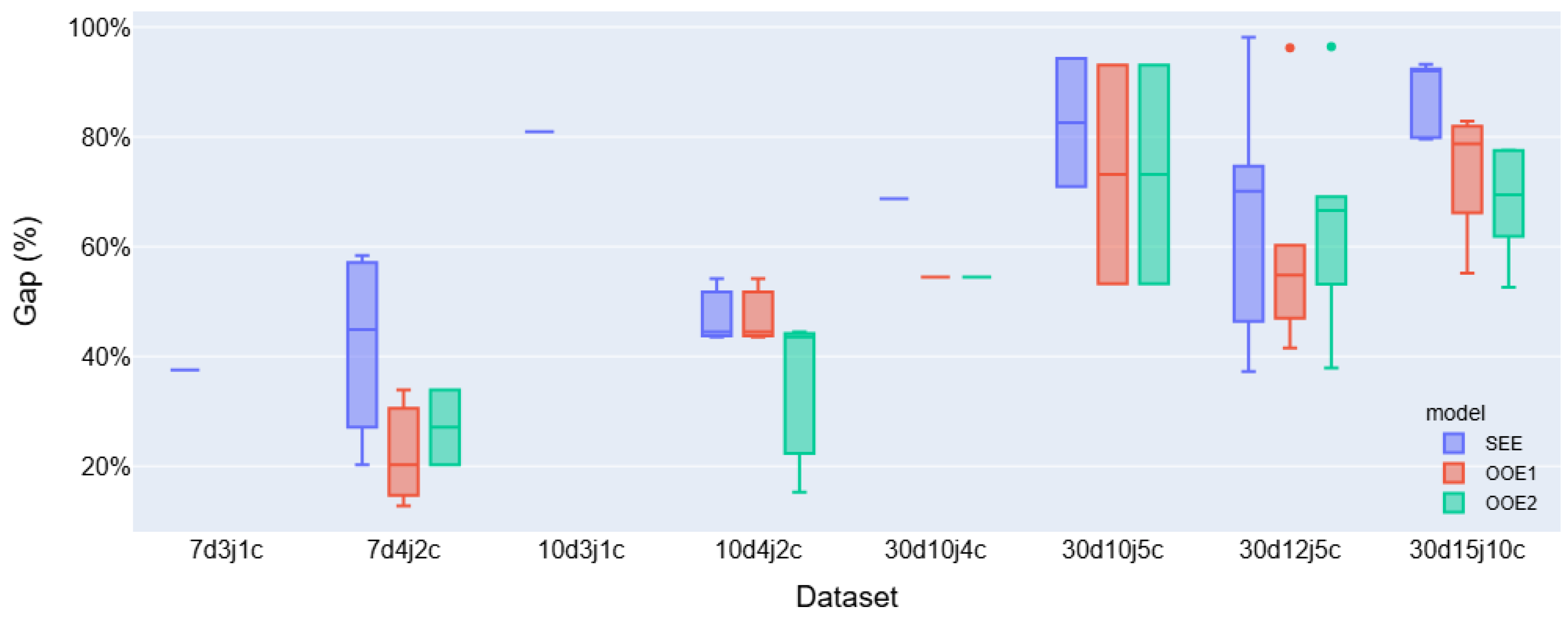
Table 8 presents the number of instances solved to optimality for each model and scenario combination within the 3600 s time limit, together with their average, minimum, and maximum solution times (in seconds). Table 9 summarizes results for the instances where optimal solutions were not obtained within the time limit. Column #proven shows the number of runs where a feasible solution was found and a strictly positive lower bound was obtained, giving a meaningful optimality gap. The average, minimum, and maximum reported gaps of these instances are also summarized in the table. Instances where the solver terminated with a feasible solution but without a proven optimality bound, including cases where the best lower bound remained zero (resulting in a reported 100% gap), are counted in the #other column.

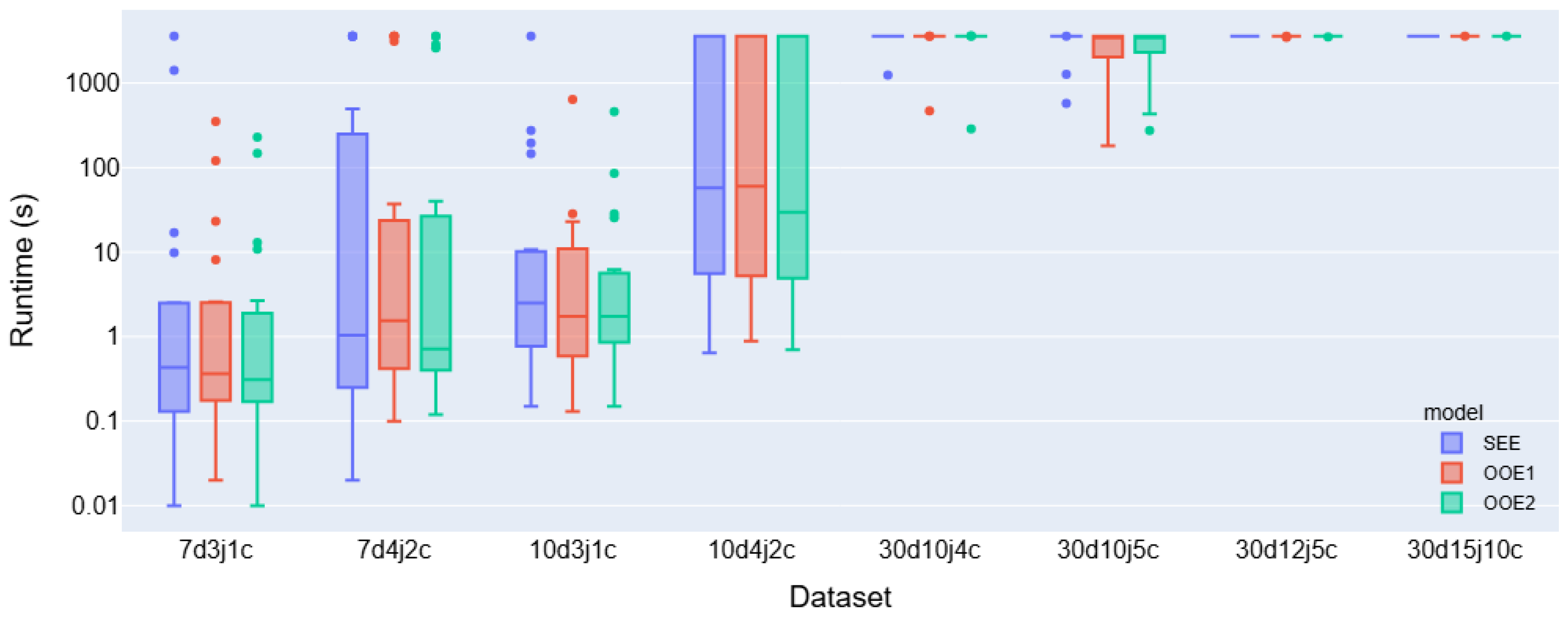
It can be seen from Table 8 and Table 9 that both OOE variants outperform the SEE model in terms of the number of optimally solved instances, especially for the more difficult scenarios. This is also true for average solution times for the optimally solved instances, and average gaps for the suboptimal ones. The same observations can be made from a more detailed analysis of the running times and gaps. Figure 6 plots the running times of the different models on every instance of the various scenarios. Figure 7 shows the gaps of the suboptimal solutions (with gaps proven by the solver) for the different models, showing again that the OOE variants outperform SEE. Chakrabortty et al. [48] reported that the OOE model is more efficient for the original MRCPSP due to the smaller number of variables, so this was expected, and remained the same for the adapted models proposed in this work.

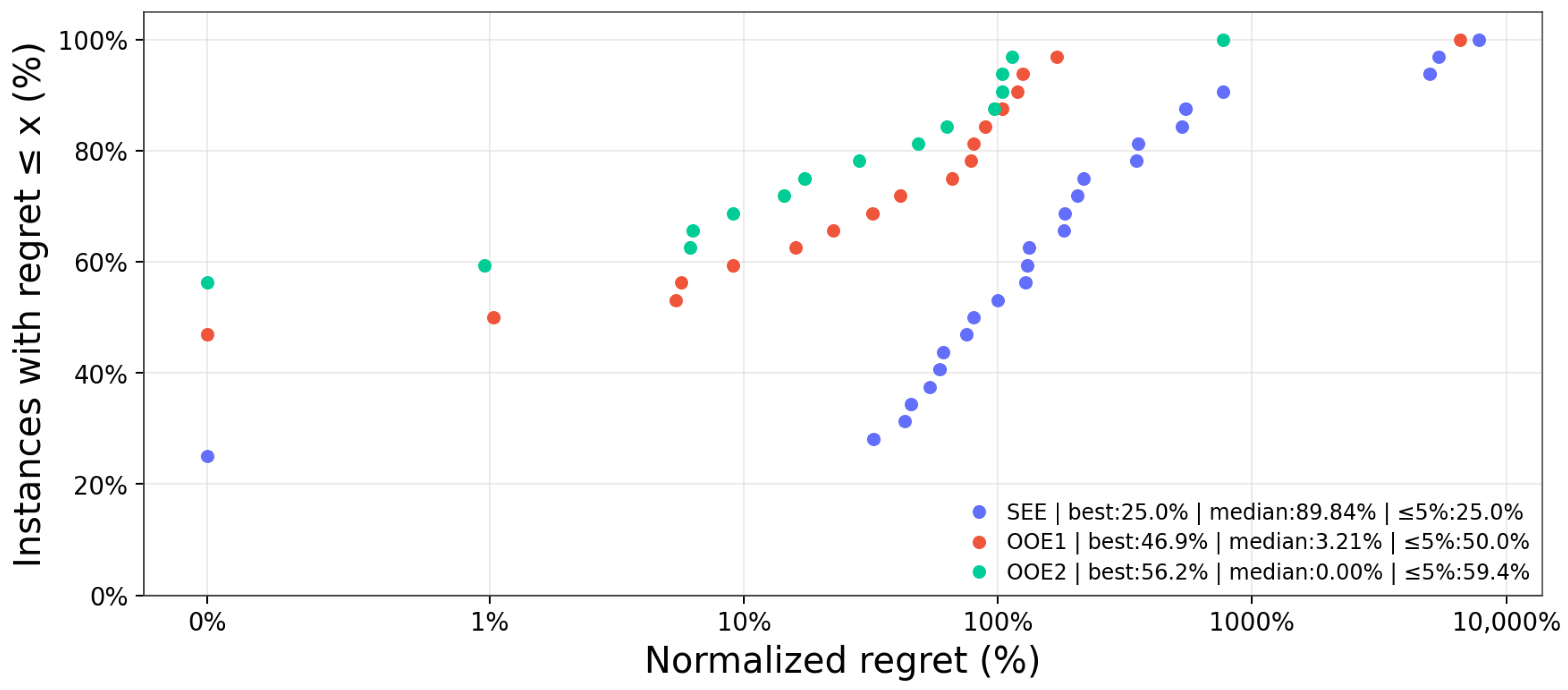
To give a more detailed analysis of the solution quality of the different models, pairwise comparisons of the obtained objective values were performed for all instances where the three models did not perform equally. Out of the 120 total instances, 32 were included in this comparison, while all models had the same objective values in the remaining 88 cases. Figure 8 shows the empirical cumulative distribution function (ECDF) of the normalized regret for the three MILP formulations on the above cases. For each instance i and model m, normalized regret was defined as:

$${\mathrm{regret}}_{i,m}={\displaystyle \frac{z_{i,m}-z_i^{\mathrm{best}}}{max\left(\left|z_i^{\mathrm{best}}\right|,1\right)}},$$

where $z_{i,m}$ is the objective value obtained by model m on instance i, and $z_i^{\mathrm{best}}$ is the best objective value among all models on i. Since the objective is to minimize total costs, lower regret values are better, and a regret of 0% indicates that the model found the best-known result for that instance. It can be seen from the ECDF that OOE2 has the best regret values overall, followed by OOE1, while SEE significantly underperforms compared to the other two models. OOE2 achieves the best objective value on 56.2% of the compared instances, followed by 46.9% for OOE1 and only 25.0% for SEE.

The tests have shown that the models can provide optimal solutions in a reasonable time for up to a 10-day planning horizon with 4 orders. As this scheduling does not need to be performed often, the solver can work on the solution for several hours, which may enable additional orders and clients or a longer time horizon. However, for even larger problems, the solution time increases steeply, and while the solver may be able to provide an incumbent solution, developing a dedicated heuristic method for the problem can be more beneficial.

5.4. Results of the GA Approach and Hyperparameter Tuning

The GA solver has several configuration parameters. Population size and the stopping criteria were determined in preliminary tests:

• Maximum number of generations: 1000;
• Population size: 3000;
• Number of elites to save for the next generation without modification: 100;
• Stop if the best solution does not improve for 100 generations;
• Stop if the average objective does not improve for 50 generations.

For other parameters, all combinations of the following values were tested:

• Crossover operator used: one-point, two-point, uniform;
• Probability of performing the crossover operation on the selected parents: 0.7, 0.9;
• Probability of performing mutation on the offspring: 0.2, 0.4, 0.6.

All parameter combinations were run 5 times on each instance to reduce the impact of the randomly generated initial population.

A stopping criterion was reached in under 60 s with all parameter settings for every instance. In most cases (in over 90%), solution time was even below 20 s.

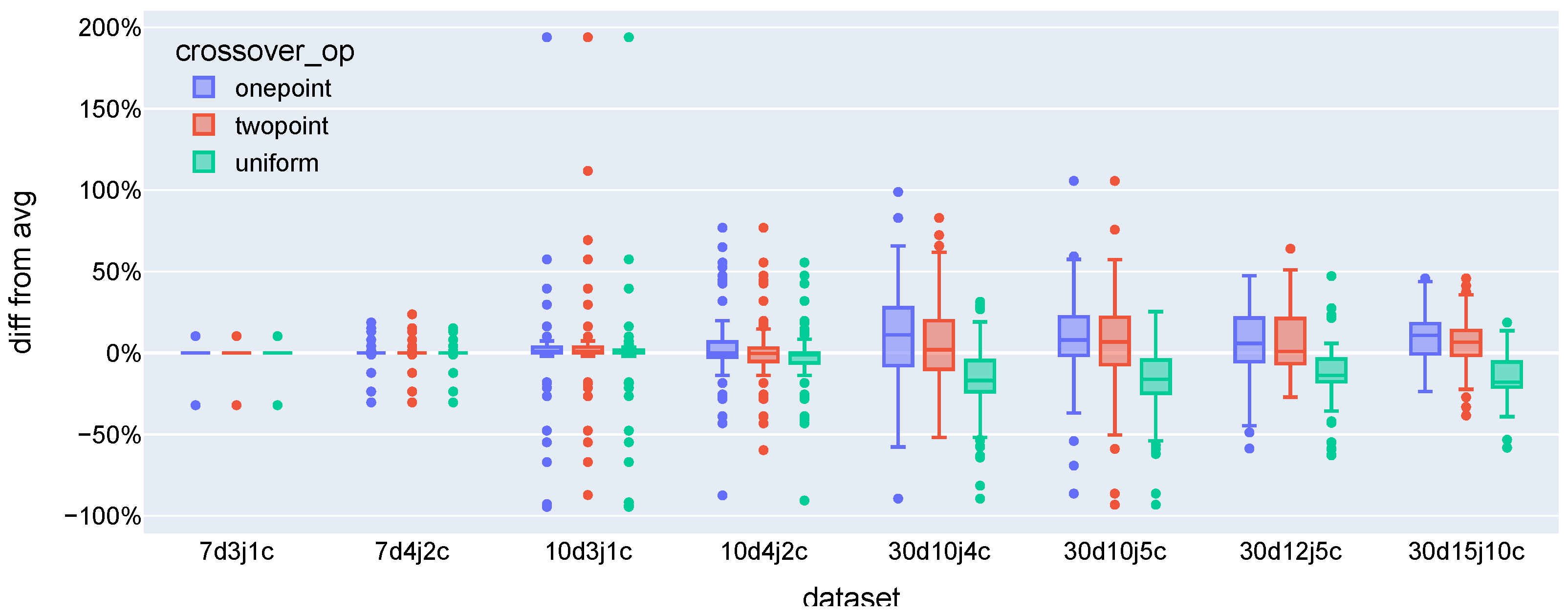
In terms of solution quality, uniform crossover performed better than other crossover operators, as shown in Figure 9. The boxplot shows the distribution of the objective values obtained in each run, relative to the average of objective values obtained on the given instance.

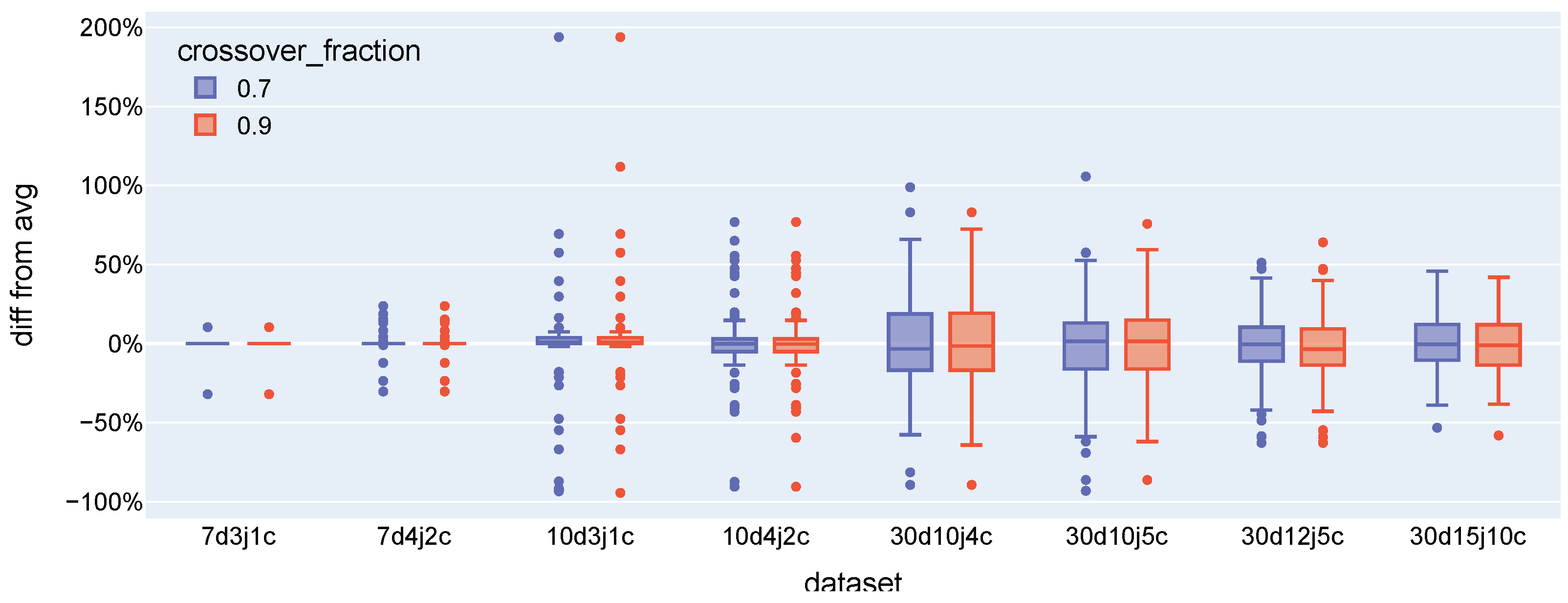
Changing the crossover probability between 0.7 and 0.9 did not noticeably affect solution quality, as shown in Figure 10.

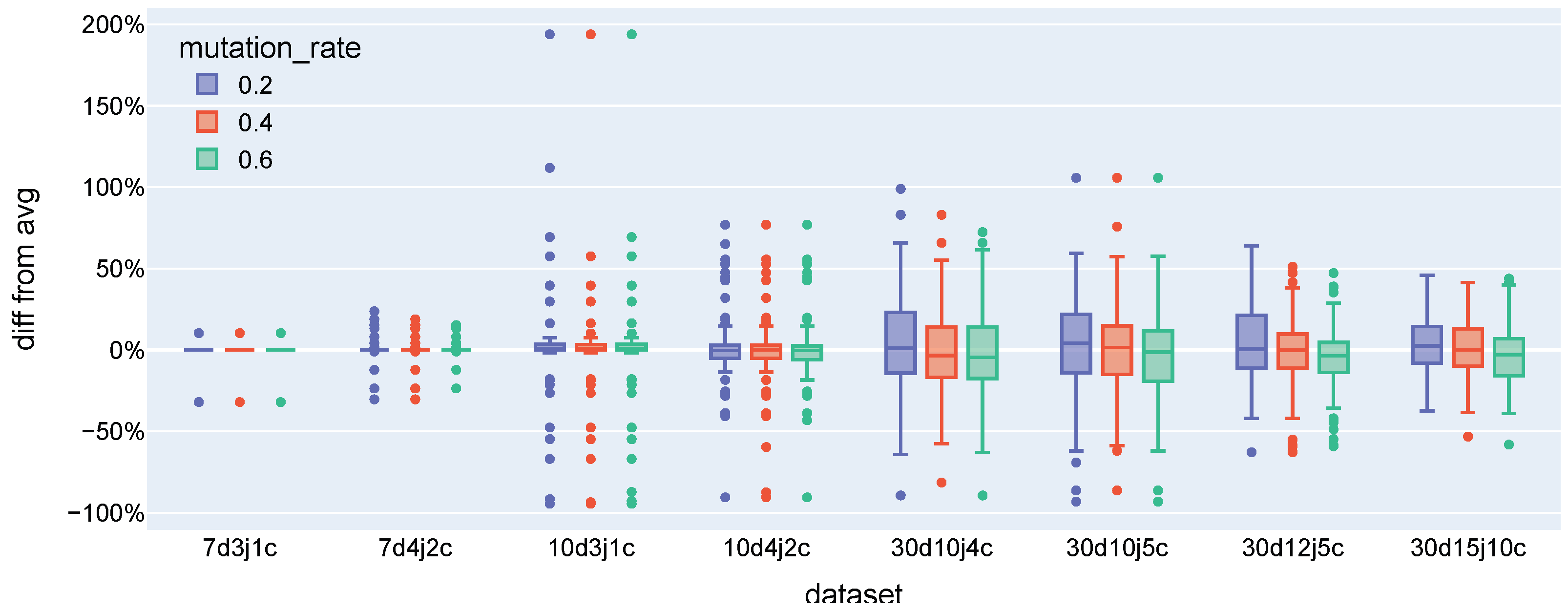
Mutation operations were helpful in finding improving solutions, so higher mutation probabilities resulted in better solution quality, as shown in Figure 11.

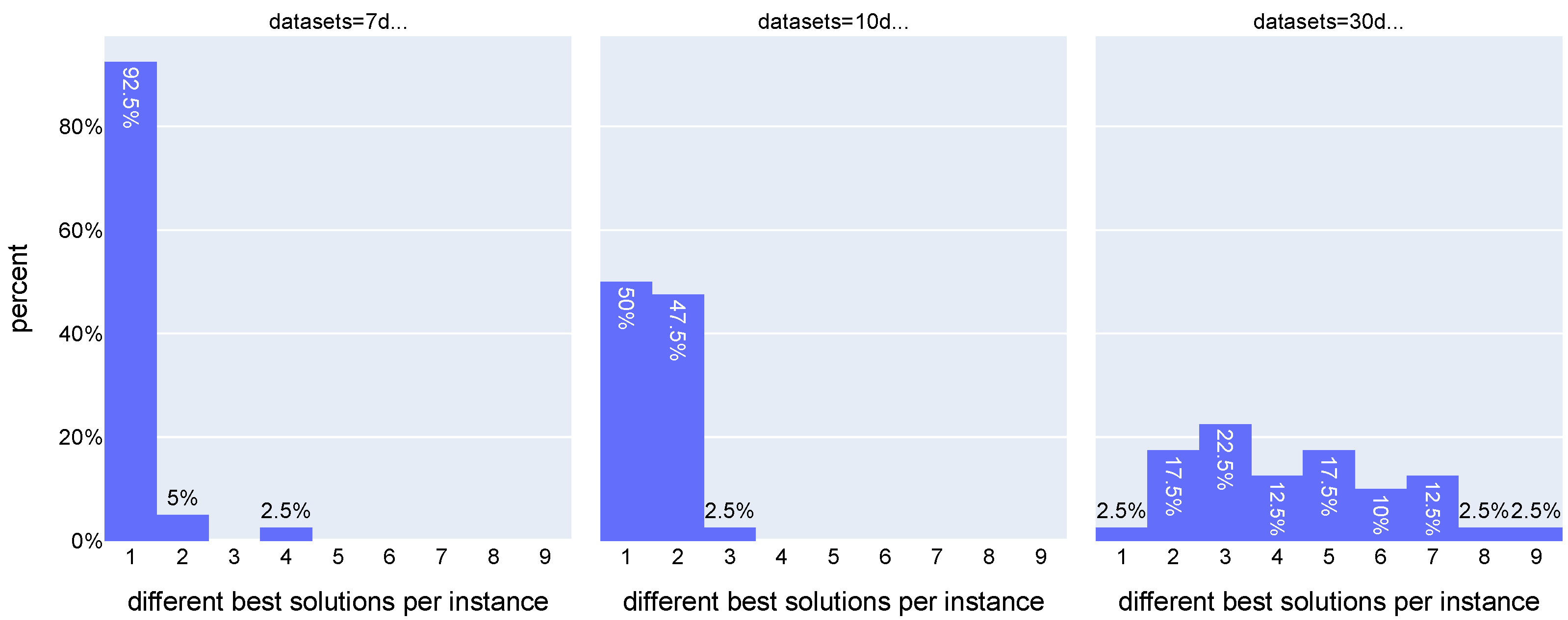
Even with the mutation and crossover operations, the algorithm can get stuck in local optima. Restarting with different initial populations can mitigate this problem. We investigated whether increasing the number of repetitions from 5 to 10 can improve the best solution found. Figure 12 shows the frequencies of the number of different objective values that the GA solver returned from 10 runs. For the small (7-day) datasets, the solver found the same solution in all 10 runs, for almost all repeated runs. For the 10-day datasets, 1 or 2 different solutions were found for most instances. In the case of the 30-day datasets, the results were less consistent: in 45% of the instances, the 10 runs resulted in 5 or more different best solutions. These results suggest that for larger problem instances, the GA approach needs more restarts to find better solutions. Based on these findings, the repetition number was increased to 15 for 30-day instances in the comparison tests of Section 5.5.

5.5. Performance Comparison

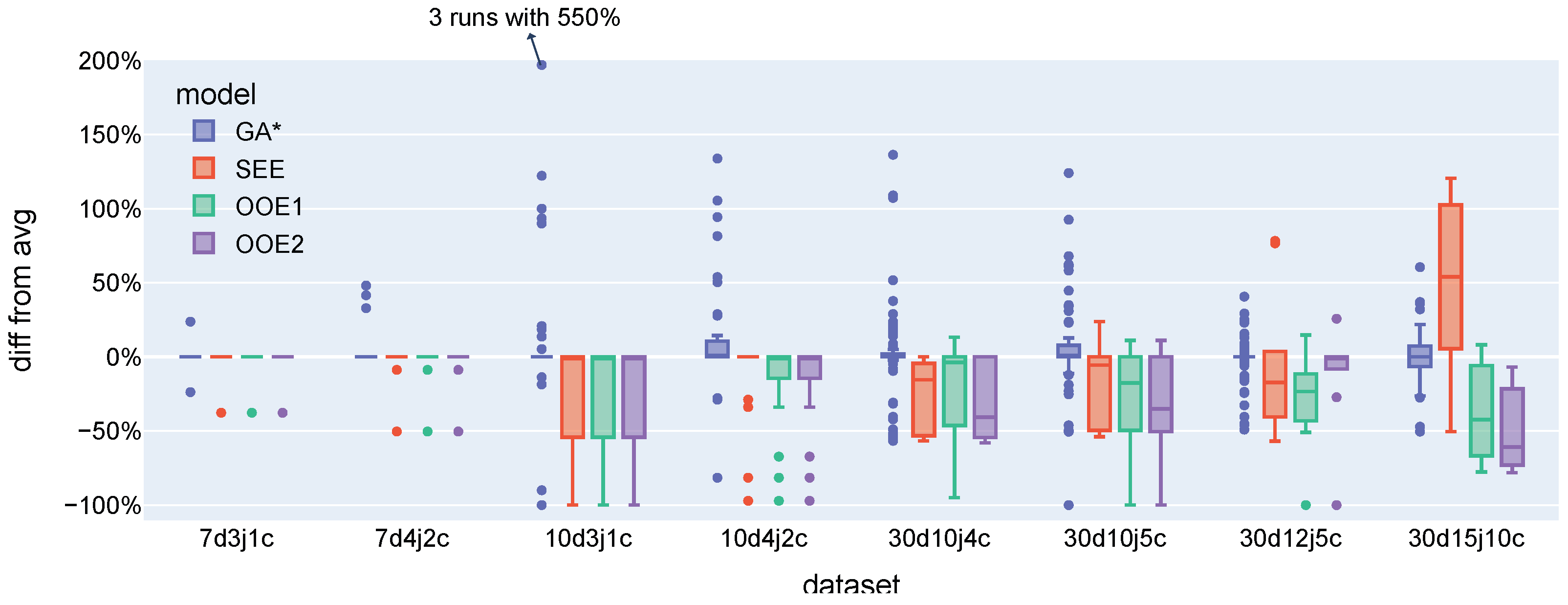
As determined in Section 5.4, the best parameter setting for the GA was uniform crossover with 0.9 probability and 0.6 mutation rate. This approach will be denoted by GA* in the following analysis. To measure its solution quality, the obtained solutions were compared to those reported by the MILP solver.

Figure 13 shows a boxplot visualizing the relative objective values compared to the average solution value of an instance. For the smaller, 7-day scenarios, GA* managed to find the optimal or best known solutions in most cases, except for at most 1–2 instances of these 20-instance datasets. For the 10-day scenarios, there was a higher variance. However, GA* was still able to find the same best solutions as the MILP solver on average.

For the 30-day scenarios, it is more informative to see how many times each approach was able to find the best solution for an instance among all approaches. This is shown by the columns under “#best” in

Table 10. Solution comparison of different approaches. #best: number of instances where the approach found the best objective value among all methods. #close: number of instances where the approach found a solution within 10% of the best known one.

Dataset		#best				#close
	SEE	OOE1	OOE2	GA*	SEE	OOE1	OOE2	GA*
7d3j1c	20	20	20	19	20	20	20	19
7d4j2c	20	20	20	18	20	20	20	19
10d3j1c	20	20	20	17	20	20	20	17
10d4j2c	19	20	20	17	19	20	20	18
30d10j4c	6	6	7	3	6	7	8	6
30d10j5c	6	7	9	8	6	7	9	8
30d12j5c	3	5	1	3	4	6	3	5
30d15j10c	0	3	7	2	0	5	9	3

. Note that GA* was executed 5 or 15 times on each instance, and the best solution among them was used (5 runs on 7–10 days datasets, 15 runs on 30-day datasets). Columns under “#close” show how many times the solution was within 10% of the best found among all methods.

While the MILP approach dominates on smaller instances that can be solved to optimality, the GA is a useful alternative for larger instances, or if a commercial MILP solver is not available. The nondeterministic nature of the GA requires several restarts to get a good quality solution, but its fast execution allows several runs in a short time.

5.6. Practical Relevance for the Industry

The presented results show that implementing deadline swapping can be a good alternative to outright cancelling customer orders in case of resource shortages. This insight can be relevant for managers, as it provides an additional tool for handling supply disruptions besides the common options of delaying or cancelling orders.

Additionally, it can be seen from the results of the mathematical models that the problem is inherently complex. While OOE2 is capable of solving most small instances to optimality within a couple of minutes, efficient runtimes are not guaranteed for larger instances, and optimality gaps could become substantial. In contrast, the GA approach can provide good-quality solutions within seconds even for larger instances. This makes it well suited for being used as a real-time decision-support tool: it can quickly generate multiple feasible solution alternatives that planners can evaluate and use as suggestions in their daily planning operations. Moreover, if time allows, the OOE2 model can still be used to validate the solutions of the heuristic, or even obtain better solutions with larger runtime limits.

Finally, although this study was motivated by the plywood manufacturing industry, the presented concepts and approaches are much more general than that. Since the formal problem definition is based on MRCPSP, the suggested approach could be adopted in other industries where temporal raw material shipments, multiple constrained resources, and flexible delivery deadlines for customer orders are relevant.

6. Conclusions

A new scheduling problem was identified in the plywood manufacturing process for mitigating supply chain disruptions and their consequences. A general formal definition was given that can be used for similar problems in other industrial and business areas. The problem was also formulated as an extended variant of the MRCPSP.

Event-based MRCPSP MILP models from the literature [48] were extended to solve the investigated problem optimally for short-term scenarios. For larger problem instances, a genetic algorithm solution approach was developed and tested for different parameter settings.

The proposed solution methods were compared on randomly generated instances. On smaller instances, the MILP models were solved to optimality, validating the mostly good solution qualities of the GA approach. For larger instances, which could not be solved to proven optimality in under 1 h, the OOE models performed better than others on average, obtaining the best quality solutions in most cases through the heuristics of the Gurobi solver.

The GA approach can quickly provide good solutions even for larger problem instances. This is useful in practical applications in production planning, for determining acceptable deadlines and planning material supply shipments. However, if given enough time, MILP models can obtain better solutions even for larger instances where optimality could not be proven.

Future research in metaheuristic approaches could improve the search procedure by applying more sophisticated methods to escape local optima instead of simple restarts. In addition, the role of the decoding process within the proposed GA framework deserves further investigation. While the current decoding mechanism is specifically designed to ensure feasibility and efficient evaluation, alternative decoding strategies could influence both solution quality and convergence behavior. A systematic comparison of different decoding methods, as well as their interaction with chromosome representation and genetic operators, would provide valuable insights into the robustness and generalizability of the approach. Exploring adaptive or problem-specific decoding schemes may further enhance performance, particularly for larger or more complex instances. Another potential topic for future research is to combine the MILP formulation with heuristic search in a hybrid solution approach, to take advantage of both methodologies.