Inverse Problem of Heat Conduction in a Multilayer Cylindrical System

Abstract

This study investigates steady-state heat transfer in a three-layer cylindrical system with angular non-uniformity of the temperature field. For the considered geometry, a mathematical model of heat conduction is formulated in cylindrical coordinates with piecewise constant thermophysical properties and continuity conditions at the interfaces between layers. The direct problem is solved analytically using a Fourier series expansion of the temperature field with respect to the angular coordinate. Based on experimental temperature measurements obtained for various configurations of soil layers, an inverse problem is formulated and solved to reconstruct the thermal conductivities of the individual layers and the heat transfer coefficient at the external boundary. To stabilize the solution, a regularized least-squares approach is employed. The convergence of the recovered parameters with respect to the harmonic number is analyzed, and the averaged reconstructed values are compared with the exact parameters used in the direct problem. The obtained results demonstrate the stability and accuracy of the proposed method, confirming its applicability to the identification of thermophysical parameters in multilayer soil systems based on experimental data.

1. Introduction

Heat transfer in heterogeneous and multilayer media constitutes a fundamental problem in a broad range of engineering and applied disciplines, including the analysis of thermal regimes in soils, building structures, thermal insulation systems, and underground infrastructure [1]. A rigorous and accurate description of heat conduction in such media is essential not only for the reliable prediction of temperature fields but also for the inverse determination of thermophysical parameters based on experimental observations [2].

The fundamental principles of heat conduction and heat and mass transfer have been comprehensively presented in classical textbooks and monographs [1,3]. These works establish the governing equations of heat transfer, outline both analytical and numerical solution techniques, and provide extensive reference data on the thermophysical properties of various materials. Collectively, they form the theoretical foundation for the development of more advanced models describing heat transfer processes in heterogeneous and inhomogeneous media. A rigorous mathematical description of heat transfer processes is formulated within the framework of the equations of mathematical physics [4]. In particular, the heat conduction equation serves as a fundamental model for describing temperature fields in continuous media [5,6].

In multilayer media, the analysis of heat transfer is substantially complicated by discontinuities in thermophysical properties at the interfaces between layers. Significant progress in the study of such systems has been reported in [7,8], where it has been demonstrated that the effective thermal conductivity strongly depends on the properties and configuration of the individual layers [9]. However, these studies are predominantly restricted to one-dimensional or radially symmetric formulations.

When extending the analysis to cylindrical geometries [10], classical models typically rely on the assumption of axial symmetry. Classical models in cylindrical geometries [10] often rely on the assumption of axial symmetry. This assumption simplifies the mathematical formulation. However, it is not always justified under realistic operating conditions, such as underground pipeline systems subjected to nonuniform airflow, seasonal temperature variations, asymmetric boundary heating, or localized heat sources. In such cases, angular variations in the temperature field become significant. Therefore, analytical models capable of incorporating angular inhomogeneity are important for a more realistic description of heat transfer in multilayer cylindrical systems.

Certain aspects of two-dimensional heat transfer problems in cylindrical coordinates have been addressed in [11,12]. Further progress in this direction was made in [13,14], where analytical solutions of the steady-state heat conduction equation in polar coordinates were obtained for multilayer soils. Nevertheless, a notable gap remains in the development of a comprehensive analytical solution for multilayer cylindrical systems that explicitly accounts for angular inhomogeneity in the boundary conditions and can be directly coupled with experimental data for parameter identification [15].

With regard to inverse problems [2,16], various approaches for parameter identification in multilayer media have been proposed in [17], including methods based on harmonic analysis and iterative reconstruction procedures. In particular, in [18], the thermal conductivity coefficients of multilayer media are determined using analytical solutions of the hyperbolic heat conduction equation in combination with identification techniques such as the Gauss–Newton method. Related inverse formulations for heat transfer processes in multilayer domains, including coupled heat and moisture transfer, have also been investigated in [19]. In addition, the proposed approach is informed by prior studies on numerical modeling of heat transfer processes in multilayer media, such as [20].

Classical inverse heat conduction problems are commonly stabilized by regularization techniques, including Tikhonov regularization, especially when measurement noise and the smoothing nature of the heat equation lead to ill-conditioned parameter recovery [21]. In recent years, modern optimization-based approaches have also been increasingly applied to inverse diffusion-type problems. For example, inverse problems for diffusion equations with fractional derivatives have been solved using metaheuristic optimization algorithms [22]. Hybrid deterministic–heuristic algorithms have also been developed for inverse reconstruction problems in computed tomography with incomplete data [23]. In addition, nature-inspired algorithms have been applied to computed tomography problems under incomplete measurement conditions, demonstrating their potential for stabilizing reconstruction when classical approaches become inefficient [24]. These studies show that inverse problems are now actively investigated not only by classical regularization methods, but also by modern optimization and reconstruction techniques.

However, several important limitations of existing approaches can still be identified. First, the choice of the number of Fourier harmonics is often insufficiently justified under conditions of experimental noise. Second, the sensitivity of the reconstructed thermophysical parameters to the retained spectral components is not always analyzed systematically. Third, many existing approaches rely mainly on numerical discretization, such as finite difference techniques and related schemes [25,26], which may limit the interpretability of the reconstruction process. Finally, only a limited number of studies combine an explicit analytical solution, angularly nonuniform boundary conditions, and experimental measurements within a unified inverse heat conduction framework for multilayer cylindrical media.

In contrast to existing studies, the present work combines an analytical solution with inverse parameter reconstruction and validation using experimental data under varying conditions. The contributions of the present study can be summarized as follows.

First, an analytical solution of the steady-state heat conduction problem is derived for a three-layer cylindrical system with piecewise-constant thermophysical properties and angularly nonuniform boundary conditions represented by a Fourier series.

Second, an inverse problem is formulated for estimating the thermal conductivities of the layers and the heat transfer coefficient based on experimental temperature measurements.

Third, a regularized least-squares framework is developed, incorporating Tikhonov regularization applied directly to the physical parameters to improve the stability of the reconstruction.

Unlike classical iterative approaches such as Gauss–Newton or Levenberg–Marquardt methods, the proposed approach relies on an analytical representation combined with gradient-based optimization, which improves interpretability and computational efficiency.

Fourth, the influence of the number of harmonics on the accuracy and stability of the solution is investigated, including an analysis of reconstruction errors and parameter sensitivity.

Finally, the proposed approach is validated using experimental data obtained for a multilayer soil system under different thermal conditions.

The remainder of this paper is organized as follows. Section 2 presents the mathematical formulation of the problem. Section 3 provides the analytical solution of the direct problem and examines the sensitivity of the Fourier coefficients. Section 4 outlines the experimental setup and data processing procedures. Section 5 formulates the inverse problem and describes the application of Tikhonov regularization and a gradient-based optimization method. Section 6 presents the results of parameter reconstruction and their comparison with reference values. Finally, the main conclusions are summarized in the concluding section.

2. Mathematical Formulation of the Problem

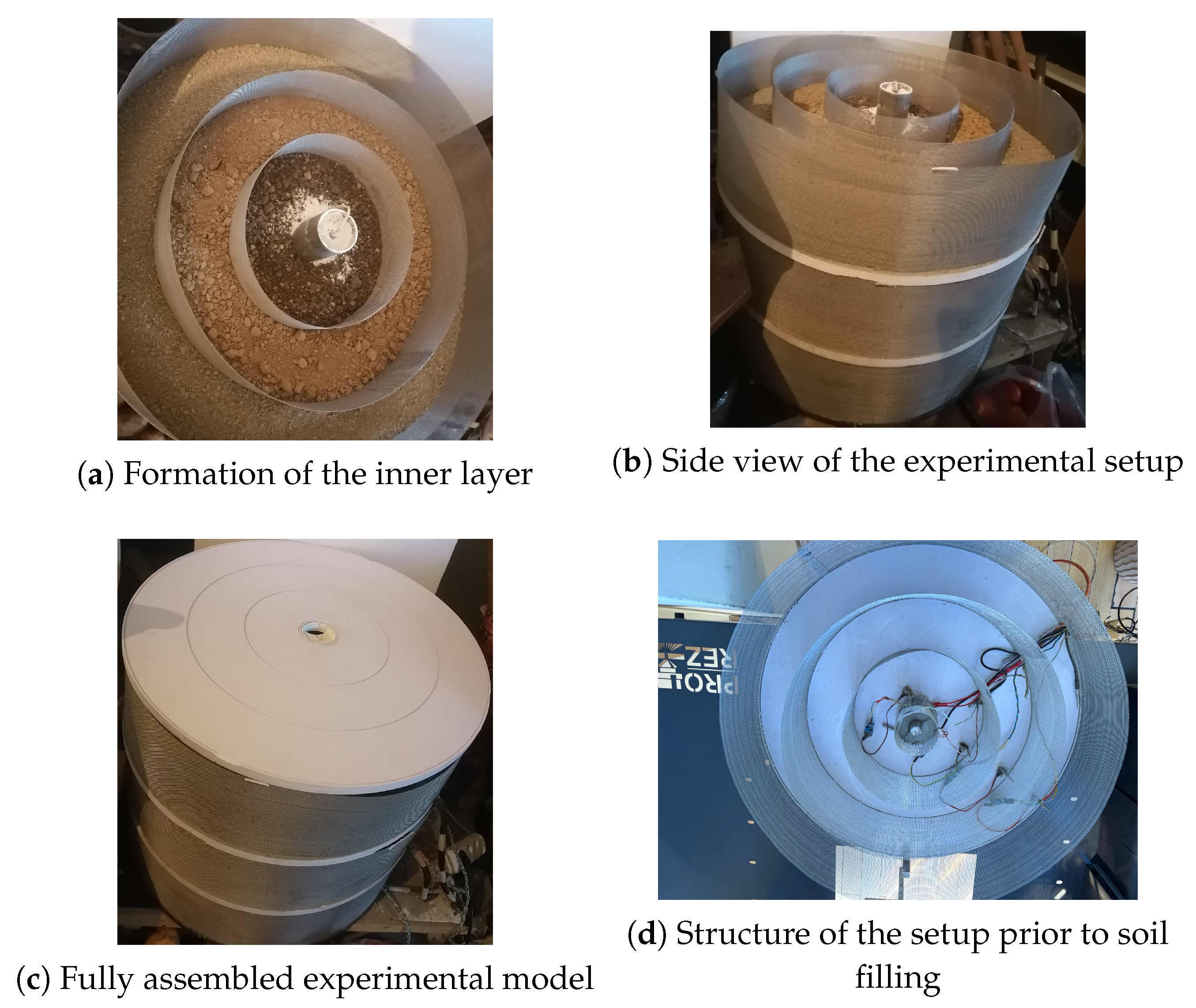
This section presents a mathematical model of steady-state heat transfer in a multilayer cylindrical system with angular nonuniformity. The model is designed to describe the experimental setup introduced in Section 4 and provides the foundation for both the direct and inverse problem formulations.

A steady-state regime is considered due to the long duration of thermal processes in the experimental system, which leads to the establishment of a quasi-stationary temperature field. Consequently, the steady-state assumption substantially simplifies the mathematical formulation, making it possible to derive analytical solutions that are essential for subsequent analysis and the identification of thermophysical parameters.

In the proposed formulation, the thermophysical properties of each layer are assumed to be piecewise constant, which represents an idealized approximation of real multilayer soil systems. In natural conditions, soil properties may vary spatially due to differences in composition, density, moisture content, and environmental influences.

2.1. Geometry of the Domain and Coordinate System

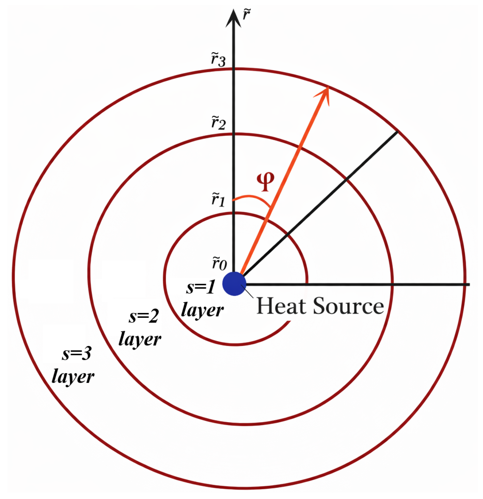
A cylindrical domain consisting of three concentric layers bounded by the radii

$${\tilde{r}}_0<{\tilde{r}}_1<{\tilde{r}}_2<{\tilde{r}}_3,$$

is considered, where $\tilde{r}$ is measured in meters $\left(m\right)$. Each layer corresponds to a distinct type of soil and is characterized by its own thermal conductivity coefficient. The temperature field is described in the cylindrical coordinate system $(\tilde{r},\phi )$, where $\tilde{r}$ denotes the radial coordinate $\left(m\right)$ and $\phi \in [0,2\pi )$ is the angular coordinate ($rad$). The schematic of the computational domain is presented in Figure 1.

The temperature field is assumed to be periodic with respect to the angular coordinate:

$$\tilde{T}(\tilde{r},\phi )=\tilde{T}(\tilde{r}\phi +2\pi ),$$

(1)

where the dimensional temperature $\tilde{T}$ is measured in Kelvin (K).

The filling of the cylindrical structure with different soil types enables the reproduction of a multilayer configuration representative of real geological media and allows for the incorporation of variations in thermophysical properties across layers. This aspect is essential for the adequate modeling of heat transfer processes under conditions that are close to natural environment. Such a formulation is commonly employed, for example, in the analysis of heat exchange around underground pipelines, geothermal boreholes, and buried cable systems [8,27].

2.2. Heat Transfer Equation

Under the assumption of steady-state heat transfer and in the absence of internal heat sources, the temperature in each layer satisfies the Laplace equation in cylindrical coordinates:

$${\displaystyle \frac{{\partial }^2\tilde{T}}{\partial {\tilde{r}}^2}}+{\displaystyle \frac{1}{\tilde{r}}}{\displaystyle \frac{\partial \tilde{T}}{\partial \tilde{r}}}+{\displaystyle \frac{1}{{\tilde{r}}^2}}{\displaystyle \frac{{\partial }^2\tilde{T}}{\partial {\phi }^2}}=0,{\tilde{r}}_0<\tilde{r}<{\tilde{r}}_3,0<\phi <2\pi .$$

(2)

This equation is formulated separately in each layer, where the thermal conductivity coefficients are assumed to be constant within a given layer but may differ between layers. The thermal conductivity coefficients $k_s$ are measured in W/(m·K).

2.3. Boundary and Interface Conditions

At the inner boundary of the cylindrical domain $\tilde{r}={\tilde{r}}_0$ the temperature is given as

$${\tilde{T}}^{\left(1\right)}({\tilde{r}}_0,\phi )=f\left(\phi \right),$$

(3)

where the function $f\left(\phi \right)$ is specified in Kelvin (K) and is determined by the experimental conditions. In the present study, the temperature at the inner boundary is assumed to be constant [28].

At the interfaces between the layers $\tilde{r}={\tilde{r}}_1$ and $\tilde{r}={\tilde{r}}_2$ continuity conditions are imposed to ensure the physical continuity of temperature and heat flux [29]:

$${\tilde{T}}^{\left(s\right)}({\tilde{r}}_s,\phi )={\tilde{T}}^{(s+1)}({\tilde{r}}_s,\phi ),$$

(4)

$$k_s{\displaystyle \frac{\partial {\tilde{T}}^{\left(s\right)}}{\partial \tilde{r}}}({\tilde{r}}_s,\phi )=k_{s+1}{\displaystyle \frac{\partial {\tilde{T}}^{(s+1)}}{\partial \tilde{r}}}({\tilde{r}}_s,\phi ),s=1,2,$$

(5)

where $k_s$—denotes the thermal conductivity of the s-th layer (W/(m·K)), and the heat flux has units of W/m².

At the outer boundary $\tilde{r}={\tilde{r}}_3$, a Robin boundary condition is imposed to describe heat exchange with the surrounding environment [30,31]:

$${\displaystyle \frac{\partial \tilde{T}}{\partial \tilde{r}}}{|}_{\tilde{r}={\tilde{r}}_3}=-{\displaystyle \frac{h}{k_3}}\left(\tilde{T}({\tilde{r}}_3,\phi )-{\tilde{T}}_a\left(\phi \right)\right),$$

(6)

where h is the convective heat transfer coefficient (W/(m²$·$K)), and ${\tilde{T}}_a\left(\phi \right)$ represents the ambient temperature (K), which may exhibit angular nonuniformity. In real soil systems, local heterogeneity and moisture-dependent variability may additionally influence the effective thermal conductivity and the overall heat transfer behavior.

2.4. Dimensionless Form of the Problem

To facilitate the analysis and subsequent numerical solution, dimensionless variables are introduced. The radial coordinate is normalized by the outer radius of the cylinder:

$$r={\displaystyle \frac{\tilde{r}}{{\tilde{r}}_3}},{\displaystyle \frac{{\tilde{r}}_0}{{\tilde{r}}_3}}<r\le 1.$$

The temperature is represented in dimensionless form $\left(T\right)$ using a reference temperature chosen for normalization:

$$T={\displaystyle \frac{\tilde{T}-T_{\mathrm{ref}}}{T_{\mathrm{ref}}}},T_{\mathrm{ref}}=277K.$$

(7)

Here, $T_{\mathrm{ref}}$ is a fixed reference temperature introduced to scale the temperature field and to obtain a dimensionless representation [32,33].

In dimensionless variables, the heat conduction equation retains the form of the Laplace equation:

$${\displaystyle \frac{{\partial }^{2}T}{\partial r^2}}+{\displaystyle \frac{1}{r}}{\displaystyle \frac{\partial T}{\partial r}}+{\displaystyle \frac{1}{r^2}}{\displaystyle \frac{{\partial }^{2}T}{\partial {\phi }^2}}=0,$$

(8)

while the Robin boundary condition at the external boundary is written in terms of the dimensionless Biot number [34]:

$${\displaystyle \frac{\partial T}{\partial r}}{|}_{r=1}=-\mathrm{Bi}\left(T(1,\phi )-T_a\left(\phi \right)\right),\mathrm{Bi}={\displaystyle \frac{h{r}_3}{k_3}},T_a\left(\phi \right)={\displaystyle \frac{{\tilde{T}}_a\left(\phi \right)-T_{\mathrm{ref}}}{T_{\mathrm{ref}}}}.$$

(9)

The remaining boundary conditions (3)–(5) remain unchanged in form after the nondimensionalization. Thus, the dimensionless formulation of the problem is governed by the geometric parameters $r_0,r_1,r_2$, the thermal conductivities of the layers $k_1,k_2,k_3$ and the Biot number $\mathrm{Bi}$.

2.5. Direct Problem Formulation

The direct heat conduction problem consists in determining the temperature field $T(r,\phi )$ in the domain $r_0<r<1$, $0<\phi <2\pi$, for given thermophysical parameters of the layers $k_1,k_2,k_3$, the heat transfer parameter (Biot number) $\mathrm{Bi}$, the temperature distribution at the inner boundary $f\left(\phi \right)$, and the ambient temperature $T_a\left(\phi \right)$.

The temperature field is governed by the heat conduction equation in polar coordinates, supplemented by appropriate boundary and interface conditions.

The solution of the direct problem serves as the basis for analyzing the thermal behavior of the system and is used to estimate model data for the inverse problem aimed at reconstructing thermophysical parameters from temperature measurements.

3. Analytical Solution of the Direct Heat Conduction Problem

In this section, the solution of the direct heat conduction problem for a multilayer cylindrical system with angular inhomogeneity is considered. The direct problem consists in determining the temperature field under given thermophysical properties of the layers and prescribed boundary conditions.

3.1. Parameters Used in the Calculations

To ensure reproducibility of the results,

Table 1. Geometric and thermophysical parameters.

Parameter	Symbol	Value	Unit	Description
Inner radius	${\tilde{r}}_0$	$0.017$	m	Inner boundary
Interface radius	${\tilde{r}}_1$	$0.070$	m	Interface between L. 1–2
Interface radius	${\tilde{r}}_2$	$0.170$	m	Interface between L. 2–3
Outer radius	${\tilde{r}}_3$	$0.270$	m	Outer boundary
Thermal conductivity of L.1	$k_1$	$0.35$	W/(m·K)	Inner layer
Thermal conductivity of L.2	$k_2$	$0.61$	W/(m·K)	Middle layer
Thermal conductivity of L.3	$k_3$	$0.70$	W/(m·K)	Outer layer
Heat transfer coefficient	h	$5.5$	W/(m2·K)	Boundary heat exchange

summarizes the numerical values of the geometric and thermophysical parameters employed in the solution of the direct problem.

All computations were performed using dimensionless variables, where the radial coordinate is given by $r=\tilde{r}/{\tilde{r}}_3$.

The thermophysical parameters listed in Table 1 were selected based on reference data for typical soil materials reported in the literature. In particular, the chosen values of thermal conductivity correspond to representative ranges for sandy, black, and clay soils under normal moisture conditions. The heat transfer coefficient at the outer boundary is also consistent with standard values used for convective heat exchange in soil–air systems.

These parameters are not obtained from the inverse procedure but are used as reference (benchmark) values for the validation of the proposed method. The inverse problem is formulated to reconstruct these parameters from experimental temperature data, allowing the accuracy and stability of the reconstruction to be assessed.

The selected ranges of thermophysical parameters are in agreement with established reference sources on heat transfer in soils and porous media [34,35,36].

3.2. Analytical Solution via Separation of Variables

To solve the steady-state heat conduction equation, the method of separation of variables is employed [37]. The temperature field is represented as the product of radial and angular components:

$$T(r,\phi )=R\left(r\right)\Phi \left(\phi \right).$$

(10)

Substituting this representation into the Laplace Equation (8) leads to a standard eigenvalue problem in the angular coordinate and to a radial equation of Bessel type $r^2{\displaystyle \frac{d^{2}R}{d{r}^2}}+r{\displaystyle \frac{dR}{dr}}-n^{2}R=0$. Taking into account the periodicity (1) with respect to the angular coordinate $\phi$, the angular solution is expressed in terms of trigonometric functions:

$${\Phi }_n\left(\phi \right)=Y_{n}cos\left(n\phi \right)+V_{n}sin\left(n\phi \right),n=0,1,2,\dots$$

The radial component of the solution for each harmonic n in each layer is given by a linear combination of power functions:

$$R_n\left(r\right)=C_n{r}^n+D_n{r}^{-n},n\ge 1,$$

while for the zeroth harmonic:

$$R_0\left(r\right)=C_{0}lnr+D_0.$$

The coefficients $Y_n$ and $V_n$ correspond to the Fourier coefficients of the angular component, while $C_n$ and $D_n$ represent the coefficients of the radial solution. All these coefficients are determined from the prescribed boundary conditions. For convenience, in the final representation, the products of the angular and radial coefficients are combined into unified constants, resulting in the coefficients $A_n^{\left(s\right)}$ and $B_n^{\left(s\right)}$, as discussed in [38]. The explicit form of the general solution is presented in the following subsection.

3.3. General Solution in a Multilayer Domain

Taking into account the three-layer structure of the domain, the solution in each layer $s=1,2,3$ is represented in the form of a Fourier series:

$$T^{\left(s\right)}(r,\phi )=A_0^{\left(s\right)}lnr+B_0^{\left(s\right)}+{\displaystyle \sum _{n=1}^{\infty }}\left(A_n^{\left(s\right)}{r}^n+A_{-n}^{\left(s\right)}{r}^{-n}\right)cos\left(n\phi \right)+{\displaystyle \sum _{n=1}^{\infty }}\left(B_n^{\left(s\right)}{r}^n+B_{-n}^{\left(s\right)}{r}^{-n}\right)sin\left(n\phi \right).$$

(11)

The unknown coefficients of (11) expansion are determined from the boundary conditions (3)–(6) at the inner and outer boundaries, as well as from the continuity conditions (4)–(5) imposed at $r=r_1$ and $r=r_2$ which correspond to the interfaces between the layers.

3.4. Determination of the Coefficients of the Solution

Substituting the general form of the solution into the boundary and interface conditions leads to a system of linear algebraic equations for the Fourier coefficients. For each harmonic n, an independent system of equations is obtained, relating the coefficients in adjacent layers through the corresponding thermal conductivity values.

For the zeroth harmonic, the resulting system determines the logarithmic coefficients $A_0^{\left(s\right)}$ and $B_0^{\left(s\right)}$, which describe the mean temperature level in the system. For harmonics $n\ge 1$ systems of equations are solved for the pairs of coefficients $A_{\pm n}^{\left(s\right)}$ and $B_{\pm n}^{\left(s\right)}$.

The Robin boundary condition at the outer boundary introduces the dimensionless Biot number, which directly influences the magnitude of the coefficients in the outer layer and governs the intensity of heat exchange with the surrounding medium.

The evaluation of the Fourier integrals appearing on the right-hand side of the equations is performed numerically using the rectangle (midpoint) method [39], providing sufficient accuracy when a sufficiently large number of nodes is employed in the angular coordinate.

3.5. Numerical Implementation

The analytically derived expressions for the Fourier coefficients (12)–(25), obtained via the method of separation of variables, form the basis for solving the direct problem. In the computations, a finite number of harmonics $n=1,\dots ,N$ is considered, where N is chosen according to the desired accuracy of the temperature field approximation. The derivation of expressions (12)–(25) is based on the Dirichlet boundary condition (4), the continuity conditions for temperature and heat flux at the layer interfaces (5)–(6), and the Robin boundary condition (8). The resulting expressions for the Fourier coefficients are presented below:

$$A_0^{\left(2\right)}={\displaystyle \frac{1}{2\pi ·R}}\left({\int }_0^{2\pi }{T}_a\left(\phi \right)d\phi -{\int }_0^{2\pi }f\left(\phi \right)d\phi \right).$$

(12)

$$A_0^{\left(1\right)}={\displaystyle \frac{k_2}{k_1}}{A}_0^{\left(2\right)}.$$

(13)

$$A_0^{\left(3\right)}={\displaystyle \frac{k_2}{k_3}}{A}_0^{\left(2\right)}.$$

(14)

$$B_0^{\left(1\right)}={\displaystyle \frac{1}{2\pi }}{\int }_0^{2\pi }f\left(\phi \right)d\phi -A_0^{\left(1\right)}ln{r}_0.$$

(15)

$$B_0^{\left(3\right)}={\displaystyle \frac{1}{2\pi }}{\int }_0^{2\pi }{T}_a\left(\phi \right)d\phi -{\displaystyle \frac{A_0^{\left(3\right)}}{Bi}}.$$

(16)

$$B_0^{\left(2\right)}=\left({\displaystyle \frac{k_2}{k_1}}\left(ln{r}_1-ln{r}_0\right)-ln{r}_1\right)·A_0^{\left(2\right)}+{\displaystyle \frac{1}{2\pi }}{\int }_0^{2\pi }f\left(\phi \right)d\phi .$$

(17)

$$A_{-n}^{\left(2\right)}={\displaystyle \frac{1}{Q·M+S}}\left({\displaystyle \frac{Bi}{\pi }}{\int }_0^{2\pi }{T}_a\left(\phi \right)cosn\phi d\phi -Q·K·{\int }_0^{2\pi }f\left(\phi \right)·cosn\phi d\phi \right).$$

(18)

$$A_n^{\left(2\right)}=K·{\int }_0^{2\pi }f\left(\phi \right)·cosn\phi d\phi +M·A_{-n}^{\left(2\right)}.$$

(19)

$$\left\{\begin{array}{c}{A}_n^{\left(1\right)}={\displaystyle \frac{k_1+k_2}{2k_1}}{A}_n^{\left(2\right)}+{\displaystyle \frac{k_1-k_2}{2k_1}}{r}_1^{-2n}{A}_{-n}^{\left(2\right)},\hfill \\ A_{-n}^{\left(1\right)}={\displaystyle \frac{k_2-k_1}{2k_1}}{r}_1^{2n}{A}_n^{\left(2\right)}+{\displaystyle \frac{k_1+k_2}{2k_1}}{A}_{-n}^{\left(2\right)}.\hfill \end{array}\right.$$

(20)

$$\left\{\begin{array}{c}{A}_n^{\left(3\right)}={\displaystyle \frac{k_2+k_3}{2k_3}}{A}_n^{\left(2\right)}-{\displaystyle \frac{\left(k_2-k_3\right)r_2^{-2n}}{2k_3}}{A}_{-n}^{\left(2\right)},\hfill \\ A_{-n}^{\left(3\right)}=-{\displaystyle \frac{k_2-k_3}{2k_3}}{r}_2^{2n}{A}_n^{\left(2\right)}+{\displaystyle \frac{k_2+k_3}{2k_3}}{A}_{-n}^{\left(2\right)}.\hfill \end{array}\right.$$

(21)

$$B_n^{\left(2\right)}={\displaystyle \frac{1}{H-I·U}}\left({\displaystyle \frac{Bi}{\pi }}{\int }_0^{2\pi }{T}_a\left(\phi \right)sinn\phi d\phi -I·O·{\int }_0^{2\pi }f\left(\phi \right)sinn\phi d\phi \right).$$

(22)

$$B_{-n}^{\left(2\right)}=O·{\int }_0^{2\pi }f\left(\phi \right)·sinn\phi d\phi -U·B_n^{\left(2\right)}.$$

(23)

$$\left\{\begin{array}{c}{B}_n^{\left(1\right)}={\displaystyle \frac{k_1+k_2}{2k_1}}{B}_n^{\left(2\right)}+{\displaystyle \frac{k_1-k_2}{2k_1}}{r}_1^{-2n}{B}_{-n}^{\left(2\right)},\hfill \\ B_{-n}^{\left(1\right)}={\displaystyle \frac{k_1-k_2}{2k_1}}{r}_1^{2n}{B}_n^{\left(2\right)}+{\displaystyle \frac{k_1+k_2}{2k_1}}{B}_{-n}^{\left(2\right)}.\hfill \end{array}\right.$$

(24)

$$\left\{\begin{array}{c}{B}_n^{\left(3\right)}={\displaystyle \frac{k_2+k_3}{2k_3}}{B}_n^{\left(2\right)}+{\displaystyle \frac{k_3-k_2}{2k_3}}{r}_2^{-2n}{B}_{-n}^{\left(2\right)},\hfill \\ B_{-n}^{\left(3\right)}={\displaystyle \frac{k_3-k_2}{2k_3}}{r}_2^{2n}{B}_n^{\left(2\right)}+{\displaystyle \frac{k_2+k_3}{2k_3}}{B}_{-n}^{\left(2\right)}.\hfill \end{array}\right.$$

(25)

All auxiliary coefficients $R,Q,M,S,K,H,U,I,O$ required in expressions (12)–(25) are explicitly derived in Appendix A.

Numerical experiments indicate that the contribution of higher-order harmonics rapidly diminishes, and a stable approximation of the temperature distribution is achieved for moderate values of N. This behavior is attributed to the smoothing nature of the Laplace equation and the physical attenuation of high-frequency temperature variations in the soil medium.

3.6. Coefficients of the Harmonic Expansion

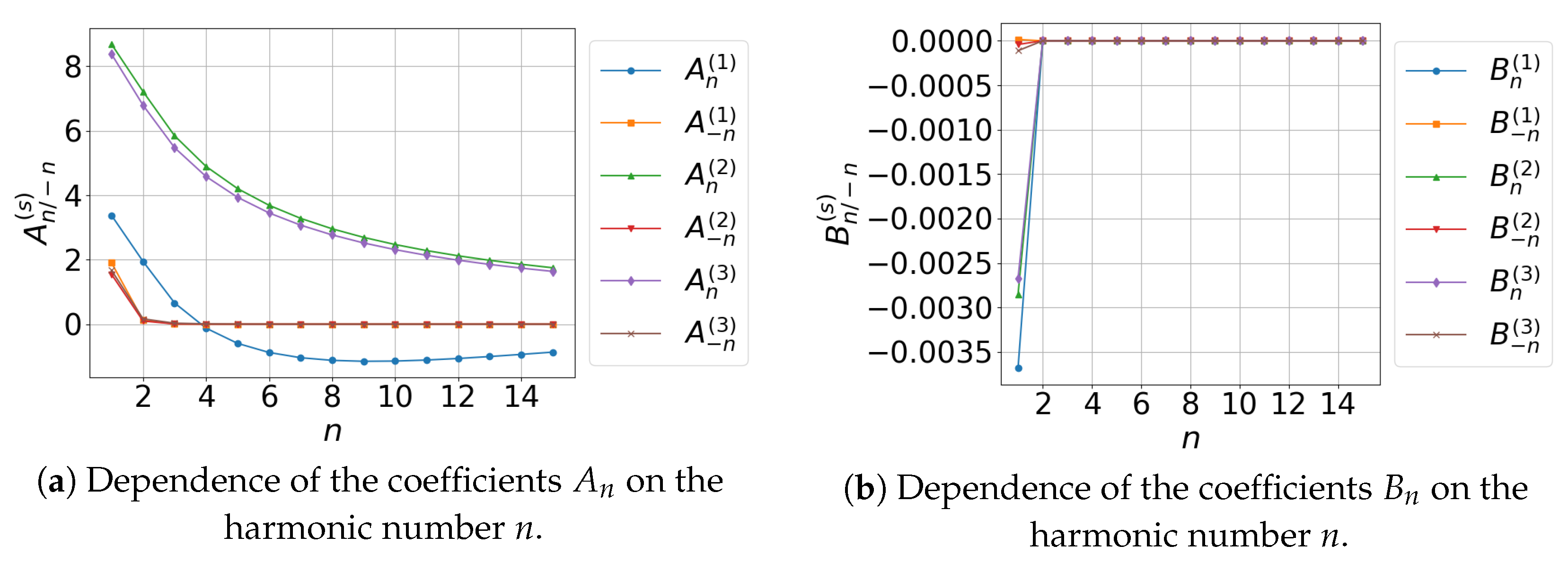
Figure 2 presents the values of the coefficients $A_n$ and $B_n$ obtained from the solution of the direct problem for the given thermophysical parameters of the system.

The analysis of the presented results shows that the absolute values of the coefficients $A_n$ and $B_n$ rapidly decrease with increasing harmonic number. This indicates that the lower-order harmonics provide the dominant contribution to the formation of the temperature field and reflects the smoothing nature of the heat conduction equation.

This property plays a crucial role in the solution of the inverse problem, as it ensures the stability of the parameter reconstruction procedure.

3.7. Sensitivity Analysis of the Coefficients with Respect to the Number of Harmonics

To assess the influence of the number of harmonics N on the stability of the spectral representation of the temperature field, a sensitivity analysis of the Fourier coefficients in each layer of the multilayer cylindrical system was performed.

The temperature field in the s-th layer is given by:

$$T_s(r,\phi )=A_{0,s}+B_{0,s}lnr+{\displaystyle \sum _{n=1}^N}\left[(A_{s,n}{r}^n+A_{s,-n}{r}^{-n})cos\left(n\phi \right)+(B_{s,n}{r}^n+B_{s,-n}{r}^{-n})sin\left(n\phi \right)\right].$$

(26)

To quantify sensitivity, a metric based on the relative contribution of additional harmonics when increasing $N_{k-1}\to N_k$ was employed:

$$S_A\left(N_k\right)={\displaystyle \frac{\parallel A_{\mathrm{add}}{\parallel }_2}{\parallel A_{1..N_k}{\parallel }_2}},S_B\left(N_k\right)={\displaystyle \frac{\parallel B_{\mathrm{add}}{\parallel }_2}{\parallel B_{1..N_k}{\parallel }_2}},$$

(27)

where

$$\parallel A_{1..N}{\parallel }_2=\sqrt{\sum _{n=1}^N\left(A_{s,n}^2+A_{s,-n}^2\right)},{\parallel B_{1..N}\parallel }_2=\sqrt{\sum _{n=1}^N\left(B_{s,n}^2+B_{s,-n}^2\right)}.$$

(28)

The quantities $A_{\mathrm{add}}$ and $B_{\mathrm{add}}$ correspond to the coefficients introduced when increasing the number of harmonics (e.g., from $N=0$ to $N=5$, then to $N=10$, etc.). The norm of the coefficients added in the transition $N_{k-1}\to N_k$ is defined as

$$\parallel A_{\mathrm{add}}{\parallel }_2=\sqrt{\sum _{n=N_{k-1}+1}^{N_k}\left(A_{s,n}^2+A_{s,-n}^2\right)}.$$

(29)

Similarly, for the $sin$ coefficients:

$$\parallel B_{\mathrm{add}}{\parallel }_2=\sqrt{\sum _{n=N_{k-1}+1}^{N_k}\left(B_{s,n}^2+B_{s,-n}^2\right)}.$$

(30)

Thus, the quantities $S_A$ and $S_B$ characterize the relative contribution of newly added harmonics to the total coefficient norm. Small values of $S_A$ and $S_B$ indicate that the solution has effectively converged with respect to the number of harmonics.

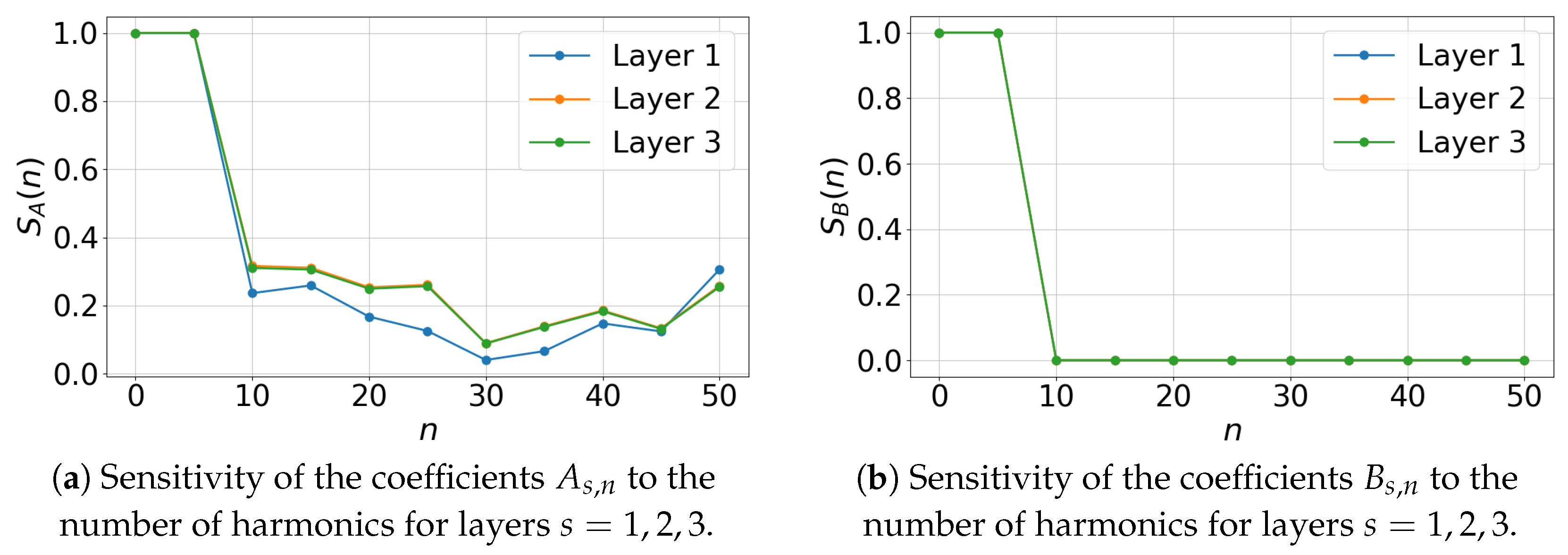
The analysis presented in Figure 3 demonstrates that, as the number of harmonics increases, the contribution of the newly added terms rapidly diminishes.

For the B-coefficients, rapid spectral stabilization is observed in all layers: already at $N\approx 10$, the contribution of higher harmonics becomes negligible.

For the A-coefficients, the decay is not strictly monotonic and exhibits noticeable fluctuations as the number of harmonics increases. This behavior is associated with the structure of the radial functions $r^{\pm n}$ and the influence of the boundary and interface conditions. The overall magnitude of the contribution decreases after the initial harmonics, local increases are observed (e.g., near $N=40$ and $N=50$), indicating that higher-order harmonics may still contribute non-negligibly.

Nevertheless, for $N\gtrsim 30$, the relative contribution of newly added harmonics remains moderate and does not significantly affect the overall spectral norm. This indicates that the spectral representation can still be regarded as sufficiently stable; the convergence is slower compared with the case of the B-coefficients.

These results confirm the stability of the spectral representation and provide a justification for selecting a finite number of harmonics in the numerical implementation of both the direct and inverse heat conduction problems.

3.8. Radial Distribution of Temperature

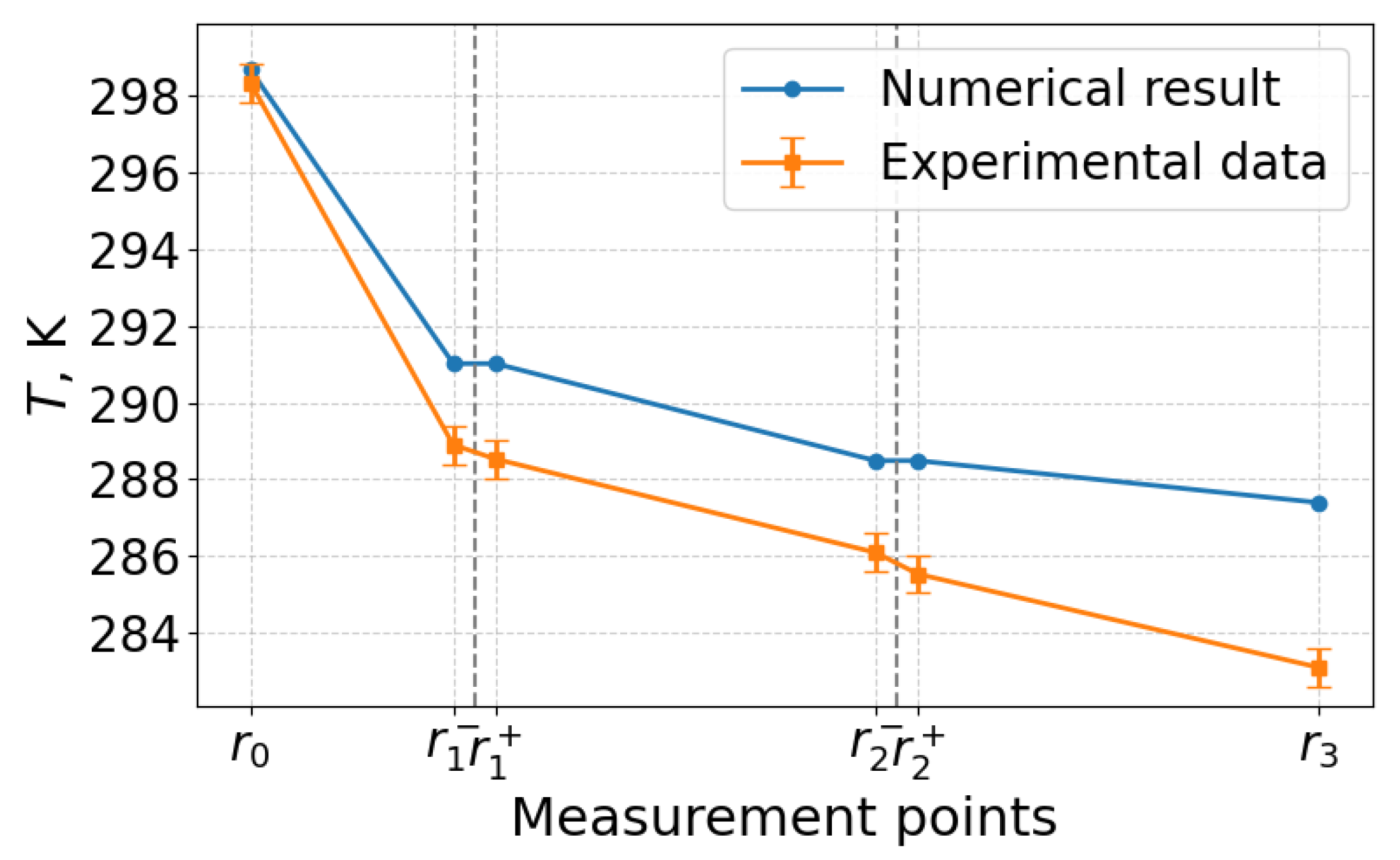
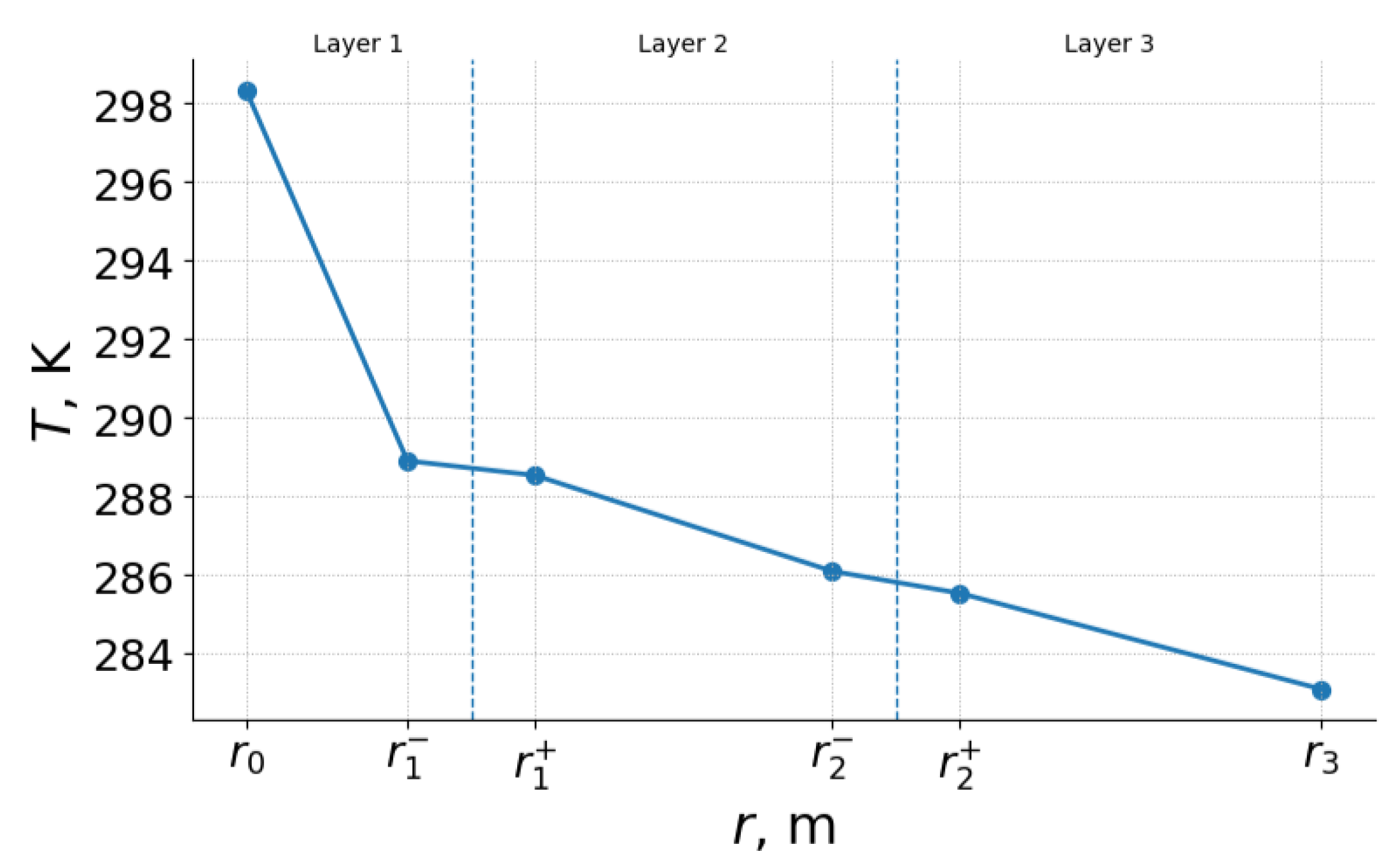
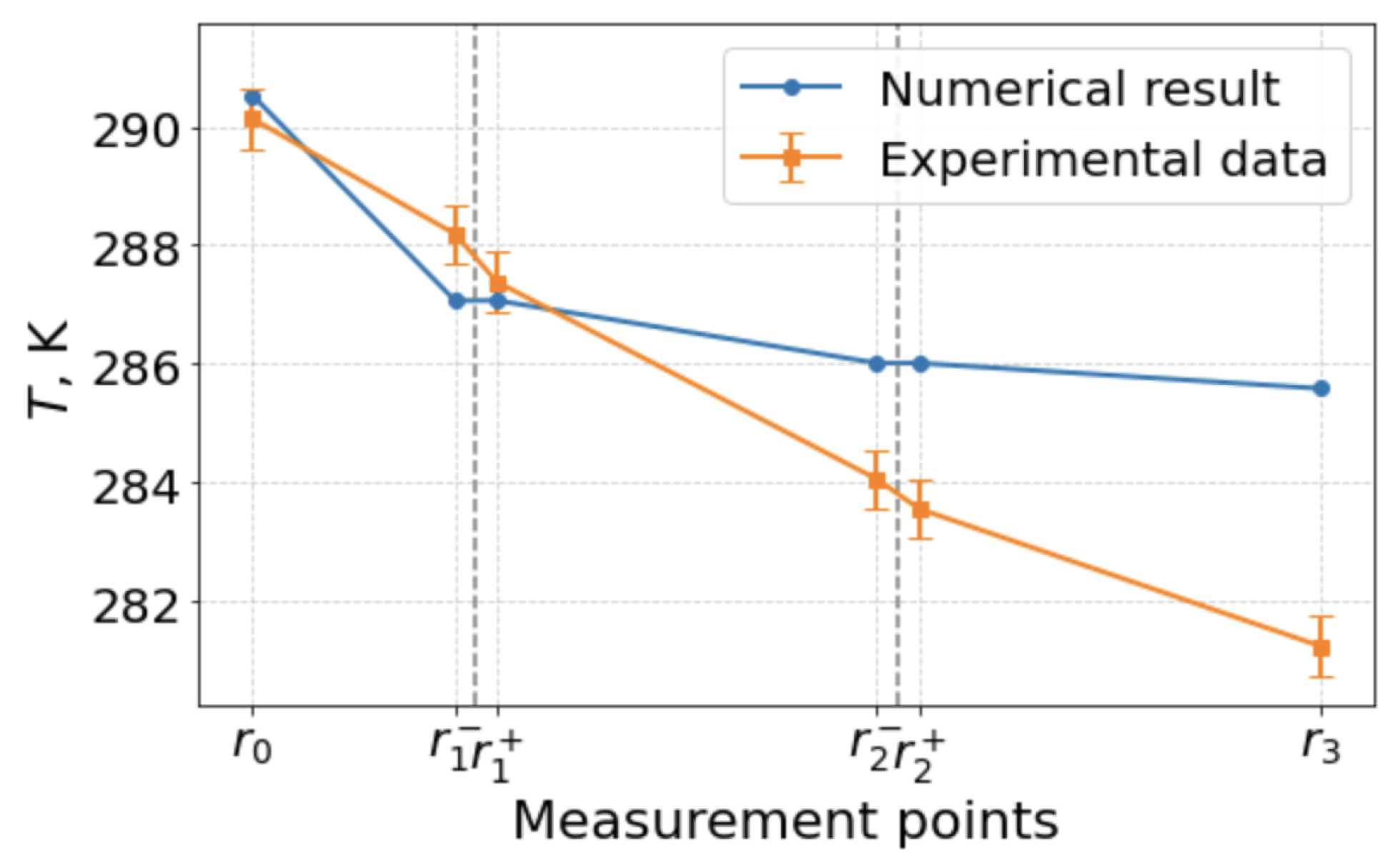
Figure 4 presents a comparison of the temperature distribution along the radial direction at a fixed angular coordinate $\phi =0$ with experimental data.

As shown in Figure 4, the temperature decreases monotonically with increasing radius. The temperature drops from approximately $298.5\mathrm{K}$ at the inner boundary $r_0$ to about $287\mathrm{K}$ near the outer boundary $r_3$. The change in slope of the curve reflects the interfaces between layers with different thermal conductivities and indicates variations in heat flux intensity. This behavior is consistent with the physical nature of steady-state heat conduction in multilayer media.

A noticeable deviation between the numerical and experimental temperature values is observed at all measurement points. The absolute difference is relatively small near the inner boundary (on the order of $0.5$–$1\mathrm{K}$) and increases toward the outer region, reaching approximately 3–$4\mathrm{K}$. In general, the numerical model tends to slightly overestimate the temperature compared with the experimental data.

Such discrepancies can be explained by several factors. First, the model assumes piecewise-constant thermophysical properties, whereas real soil exhibits spatial heterogeneity and moisture-dependent variations. Second, experimental uncertainties, including sensor accuracy and environmental influences, contribute to measurement deviations. Third, simplifications in the boundary conditions, especially in the representation of heat exchange at the outer boundary, introduce additional modeling errors. Furthermore, the increasing discrepancy toward the outer region may be attributed to the higher sensitivity of the solution to boundary conditions and external heat exchange effects in this region.

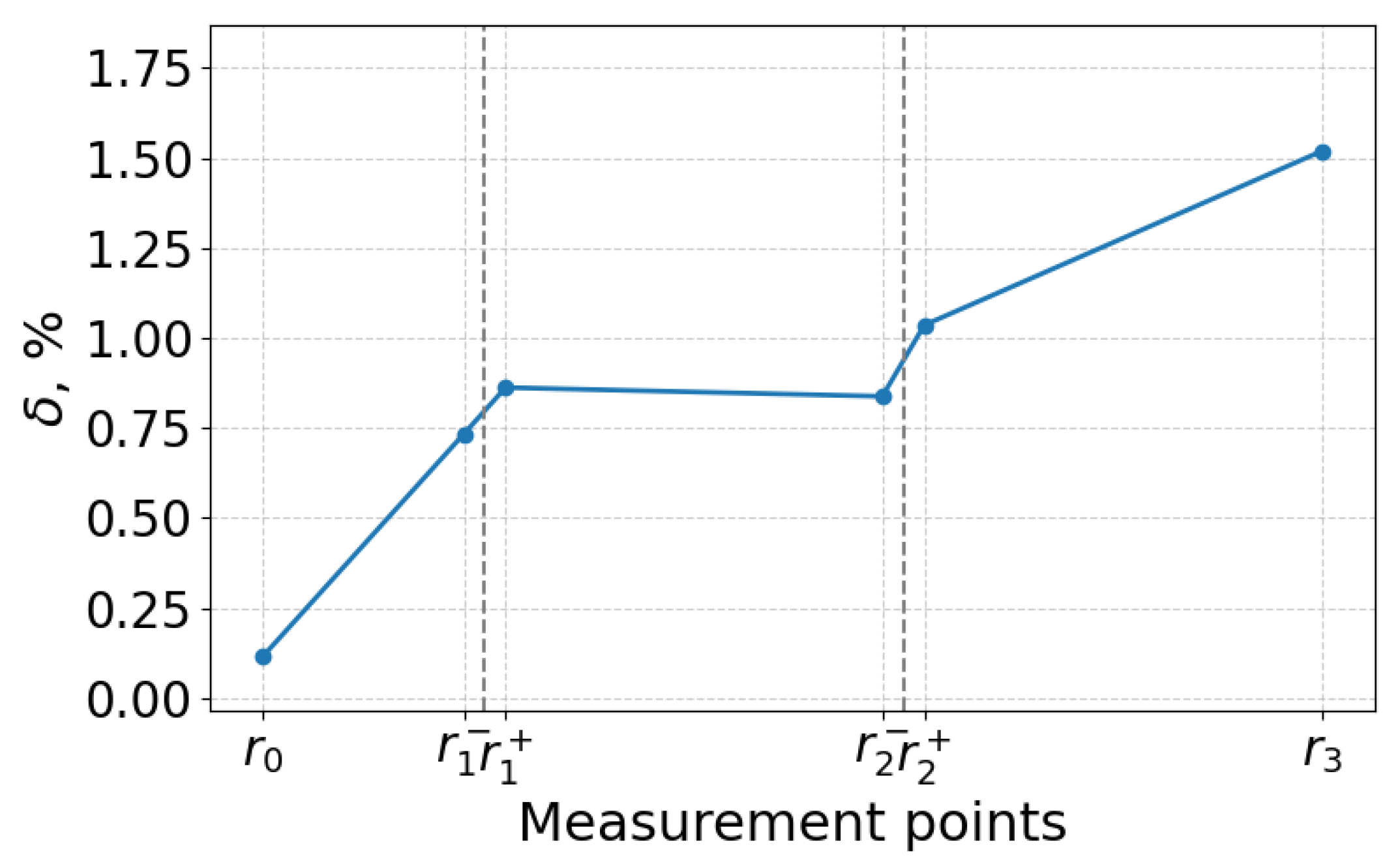
The relative error distribution shown in Figure 5 confirms the good agreement between the numerical and experimental results. The error is minimal at the inner boundary (≈0.1%), increases to about $0.7$–$0.9\%$ within the intermediate layers, and reaches a maximum of approximately $1.5\%$ near the outer boundary. This gradual increase reflects the accumulation of modeling and measurement uncertainties along the radial direction.

The relatively low magnitude of the relative error, the observed absolute differences, is explained by the high temperature level of the system (on the order of 290–$300\mathrm{K}$), where even deviations of several degrees correspond to small percentage errors. Minor fluctuations within the intermediate layers indicate the stability of the numerical method and the correct implementation of the interface conditions.

Overall, the results demonstrate good agreement between the model and the experimental data and confirm the reliability and practical applicability of the proposed approach for modeling heat transfer in multilayer media.

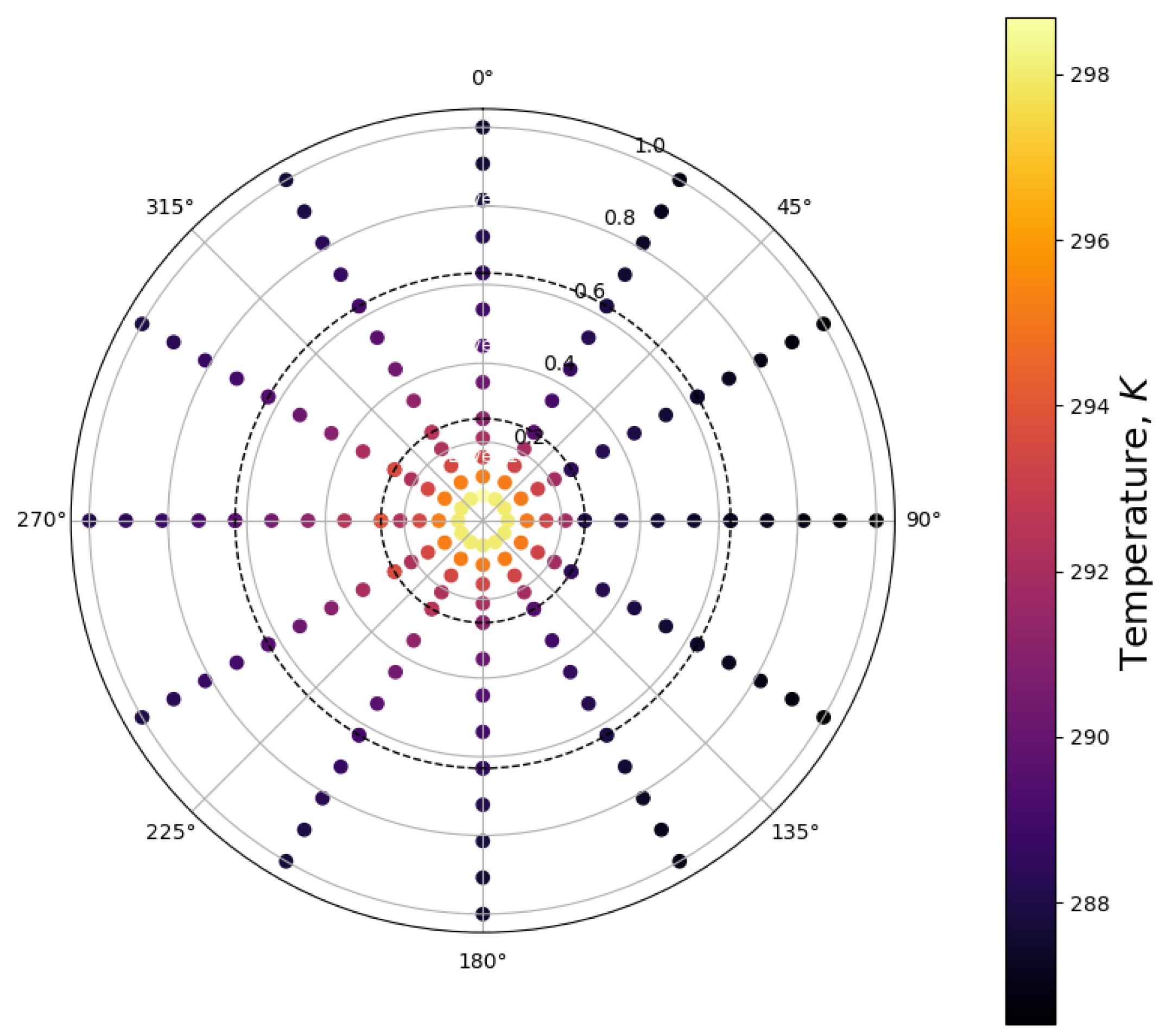
Figure 6 shows the temperature distribution obtained from the solution of the direct problem. It can be observed that the temperature field exhibits angular symmetry with respect to the principal directions, which is consistent with the imposed boundary conditions and the geometrical structure of the multilayer system.

3.9. Analysis of the Results of the Direct Problem

The results of the direct problem solution demonstrate that the use of a finite number of harmonics in the analytical representation of the temperature field allows achieving a relative error on the order of 1% with a moderate number of terms in the series. The lower-order harmonics provide the dominant contribution to the solution, while the contribution of higher-order harmonics rapidly diminishes.

The obtained temperature fields and the corresponding harmonic expansion coefficients are subsequently utilized for the formulation and solution of the inverse heat conduction problem, aimed at reconstructing the thermophysical parameters of the multilayer cylindrical system based on experimental data.

4. Experimental Model and Data

4.1. Description of the Experimental Setup

To validate the mathematical model and enable subsequent solution of the inverse heat conduction problem, a long-term in situ experiment was conducted on a multilayer cylindrical system designed to simulate the stratified structure of soil. The experimental setup consisted of a cylindrical domain filled with several layers of soil materials possessing different thermophysical properties.

In the experiment, the layers were arranged in the following order (from the inner to the outer region): river sand, chernozem (black soil), and clay.

Temperature sensors were installed along the radial direction at a fixed angular coordinate $\phi =0$. Measurements were recorded at regular time intervals of 10 min over a period of 398 days, providing representative temperature time series that capture both seasonal variations and quasi-steady thermal behavior. For the purpose of validation, a representative temperature profile corresponding to the first day of measurements is used for detailed comparison with the analytical solution in Section 3. In addition, temperature data from other time instances (days 4, 12, and 138) are employed in Section 5 to assess the robustness of the proposed inverse modeling framework under varying thermal conditions.

To ensure consistency with the mathematical model, all measured temperature values were converted to an absolute temperature scale and subsequently expressed in degrees Kelvin.

4.2. Experimental Temperature Data

The analysis of the experimental temperature profile presented in Figure 7 reveals the main features of temperature distribution in the multilayer cylindrical system. At the fixed time instant $t=12:00$, a monotonic decrease in temperature is observed as the radial coordinate increases from the inner boundary $r_0$ to the outer boundary $r_3$. This behavior is consistent with the physical nature of steady-state heat transfer, where heat propagates from the higher-temperature region in the inner layer toward the cooler external environment.

Particular attention should be paid to the temperature behavior in the vicinity of the layer interfaces at $r_1$ and $r_2$. As shown in Figure 7, the temperature values on both sides of these interfaces exhibit slight discrepancies, which may visually appear as weak discontinuities. However, a quantitative assessment indicates that these differences are small, and the temperatures on either side of each interface remain approximately equal. This suggests that the continuity condition of temperature at the layer interfaces is satisfied with good accuracy.

The observed deviations can be explained by several factors, including experimental measurement errors, the discrete nature of the data acquisition process, and possible local inhomogeneities in the thermophysical properties of the materials, especially near the interfaces. It should also be noted that in the mathematical model of steady-state heat conduction, the interface conditions are assumed to be ideal, with exact continuity of temperature. In practice, however, experimental measurements always contain small fluctuations. In addition, the total discrepancy can be attributed to three main sources: (i) modeling error arising from simplifying assumptions such as piecewise-constant thermophysical properties and idealized boundary conditions, (ii) experimental uncertainty related to sensor accuracy and environmental influences, and (iii) numerical approximation errors associated with the truncation of the Fourier series. The combined effect of these factors explains the observed deviation between the numerical and experimental results.

The experimental temperature data are affected by uncertainties related to sensor accuracy and the measurement procedure. According to the specifications of the equipment used, the absolute measurement uncertainty can be estimated as

$$\Delta T=\pm 0.5\mathrm{K},$$

(31)

based on the sensor accuracy and standard uncertainty analysis procedures [40]. To evaluate how well the numerical results agree with the experimental data, the relative error was calculated as

$${\delta }_T={\displaystyle \frac{\left|T_{\mathrm{num}}-T_{\exp }\right|}{T_{\exp }}}\times 100\%,$$

(32)

which is a commonly used measure for comparing numerical and experimental data [41]. In all considered points, the relative error does not exceed approximately $1.5\%$, which is consistent with the expected level of experimental uncertainty. This indicates that the observed differences are mainly due to measurement errors and do not affect the overall conclusions. Overall, the model shows good agreement with the experimental data and can be considered suitable for describing steady-state heat conduction in the multilayer system under study. The obtained temperature profile supports the use of the selected experimental snapshot for comparison with the analytical solution presented in Section 3. Additional experimental datasets are further utilized in Section 5 to validate the proposed approach under different temporal conditions.

Figure 8 illustrates the main stages in the construction of the experimental setup. The multilayer structure is formed sequentially using cylindrical separating shells, which ensure the preservation of layer geometry and minimize mixing between materials. The central part of the setup contains a heating element and measurement sensors, enabling the acquisition of temperature data along the radial direction.

The experimental data obtained in this study were used to define boundary conditions for the direct heat conduction problem and to formulate the inverse problem of reconstructing the thermophysical parameters of the multilayer system.

5. Formulation and Solution of the Inverse Heat Conduction Problem

In this section, the inverse heat conduction problem is considered, which consists in reconstructing the thermophysical parameters of a multilayer cylindrical system based on experimental temperature data. In contrast to the direct problem, where the thermal conductivity and heat transfer coefficients are assumed to be known, these parameters are treated as unknowns to be identified in the inverse problem.

5.1. Formulation of the Inverse Problem

The solution is given by:

$$\left\{\begin{array}{c}{T}^{\left(1\right)}(r,\phi )=A_0^{\left(1\right)}lnr+B_0^{\left(1\right)}+{\sum }_{n=1}^{\infty }(A_n^{\left(1\right)}{r}^n+A_{-n}^{\left(1\right)}{r}^{-n})cosn\phi +{\displaystyle {\sum }_{n=1}^{\infty }}(B_n^{\left(1\right)}{r}^n+B_{-n}^{\left(1\right)}{r}^{-n})sinn\phi ,\hfill \\ T^{\left(2\right)}(r,\phi )=A_0^{\left(2\right)}lnr+B_0^{\left(2\right)}+{\displaystyle {\sum }_{n=1}^{\infty }}(A_n^{\left(2\right)}{r}^n+A_{-n}^{\left(2\right)}{r}^{-n})cosn\phi +{\sum }_{n=1}^{\infty }(B_n^{\left(2\right)}{r}^n+B_{-n}^{\left(2\right)}{r}^{-n})sinn\phi ,\hfill \\ T^{\left(3\right)}(r,\phi )=A_0^{\left(3\right)}lnr+B_0^{\left(3\right)}+{\displaystyle {\sum }_{n=1}^{\infty }}(A_n^{\left(3\right)}{r}^n+A_{-n}^{\left(3\right)}{r}^{-n})cosn\phi +{\displaystyle {\sum }_{n=1}^{\infty }}(B_n^{\left(3\right)}{r}^n+B_{-n}^{\left(3\right)}{r}^{-n})sinn\phi .\hfill \end{array}\right.$$

(33)

Using the orthogonality properties of trigonometric functions, the Fourier coefficients of the temperature field at the interfaces $r=r_2$ and $r=r_3$ are obtained by integration over the angular coordinate.

The inverse problem consists in determining the thermophysical parameters

$$q={(k_1,k_2,k_3,h)}^T,$$

where $k_1$, $k_2$, and $k_3$ are the thermal conductivities of the layers, and h is the heat transfer coefficient at the outer boundary.

The experimental temperature measurements were performed along the radial direction at a fixed angular coordinate $\phi =0$. The mean temperature values at the interfaces are taken directly from the experimental data. In dimensional form, these values are

$${\tilde{T}}_2=288.38\mathrm{K},{\tilde{T}}_3=285.38\mathrm{K}.$$

Using the dimensionless transformation defined in (7), the corresponding dimensionless mean values are

$$T_2\approx 0.041,T_3\approx 0.030.$$

Since experimental measurements are available only at $\phi =0$, the angular temperature dependence cannot be directly reconstructed from the data. Therefore, a physically motivated smooth periodic approximation is introduced.

To incorporate angular nonuniformity into the analytical framework, the temperature distributions at $r=r_2$ and $r=r_3$ are approximated in the form

$$T^{\left(2\right)}\left(\phi \right)=T_2-A_{2}sin\phi ,T^{\left(3\right)}\left(\phi \right)=T_3-A_{3}sin\phi .$$

The choice of the sinusoidal angular dependence is motivated by a physically plausible asymmetric thermal forcing. In particular, it is assumed that the dominant external heat input (e.g., solar radiation) is applied from a preferential direction corresponding to $\phi ={\displaystyle \frac{\pi }{2}}$, where the temperature reaches its maximum.

Due to the periodic nature of the angular coordinate, the opposite direction $\phi ={\displaystyle \frac{3\pi }{2}}$ corresponds to the region with minimal thermal influence and thus the lowest temperature. The directions $\phi =0$ and $\phi =\pi$ represent intermediate angular positions, where the temperature is close to its mean value. In particular, at $\phi =0$, the temperature coincides with the experimentally measured value, ensuring consistency with the available data.

Such a representation corresponds to the first harmonic of the Fourier expansion and captures the dominant mode of angular variation while preserving smoothness, periodicity, and physical interpretability of the temperature field.

The amplitudes $A_2$ and $A_3$ are determined based on physically realistic temperature variations in soil systems. In practical applications involving buried cylindrical structures, asymmetric environmental conditions may lead to temperature differences along the circumference of the order of 5–15 K [42].

For the second layer, a maximum temperature decrease of approximately $11\mathrm{K}$ relative to the mean value is assumed, yielding

$${\tilde{T}}_{2,min}=288.38-11=277.38\mathrm{K}.$$

Using (7), the corresponding dimensionless amplitude is

$$A_2={\displaystyle \frac{{\tilde{T}}_{2,min}-T_{\mathrm{ref}}}{T_{\mathrm{ref}}}}\approx 0.0014.$$

Similarly, for the third layer, a temperature decrease of approximately $7.5\mathrm{K}$ is considered:

$${\tilde{T}}_{3,min}=285.38-7.5=277.88\mathrm{K},$$

which gives

$$A_3\approx 0.0034.$$

Thus, the angular temperature distributions used in the inverse problem are

$$T^{\left(2\right)}\left(\phi \right)=0.041-0.0014sin\phi ,T^{\left(3\right)}\left(\phi \right)=0.030-0.0034sin\phi .$$

The Fourier coefficients of the temperature data are computed as

$$a_n^{\left(s\right)}={\displaystyle \frac{1}{\pi }}{\int }_0^{2\pi }{T}^{\left(s\right)}(r_s,\phi )cos\left(n\phi \right)d\phi ,b_n^{\left(s\right)}={\displaystyle \frac{1}{\pi }}{\int }_0^{2\pi }{T}^{\left(s\right)}(r_s,\phi )sin\left(n\phi \right)d\phi ,s=2,3.$$

The inverse problem is formulated as a nonlinear least-squares problem:

$$J\left(q\right)=J_{\mathrm{data}}\left(q\right)+\alpha {\parallel q-q_{\mathrm{ref}}\parallel }^2,$$

where $J_{\mathrm{data}}$ is the discrepancy between the Fourier coefficients of the analytical solution and those obtained from the temperature data.

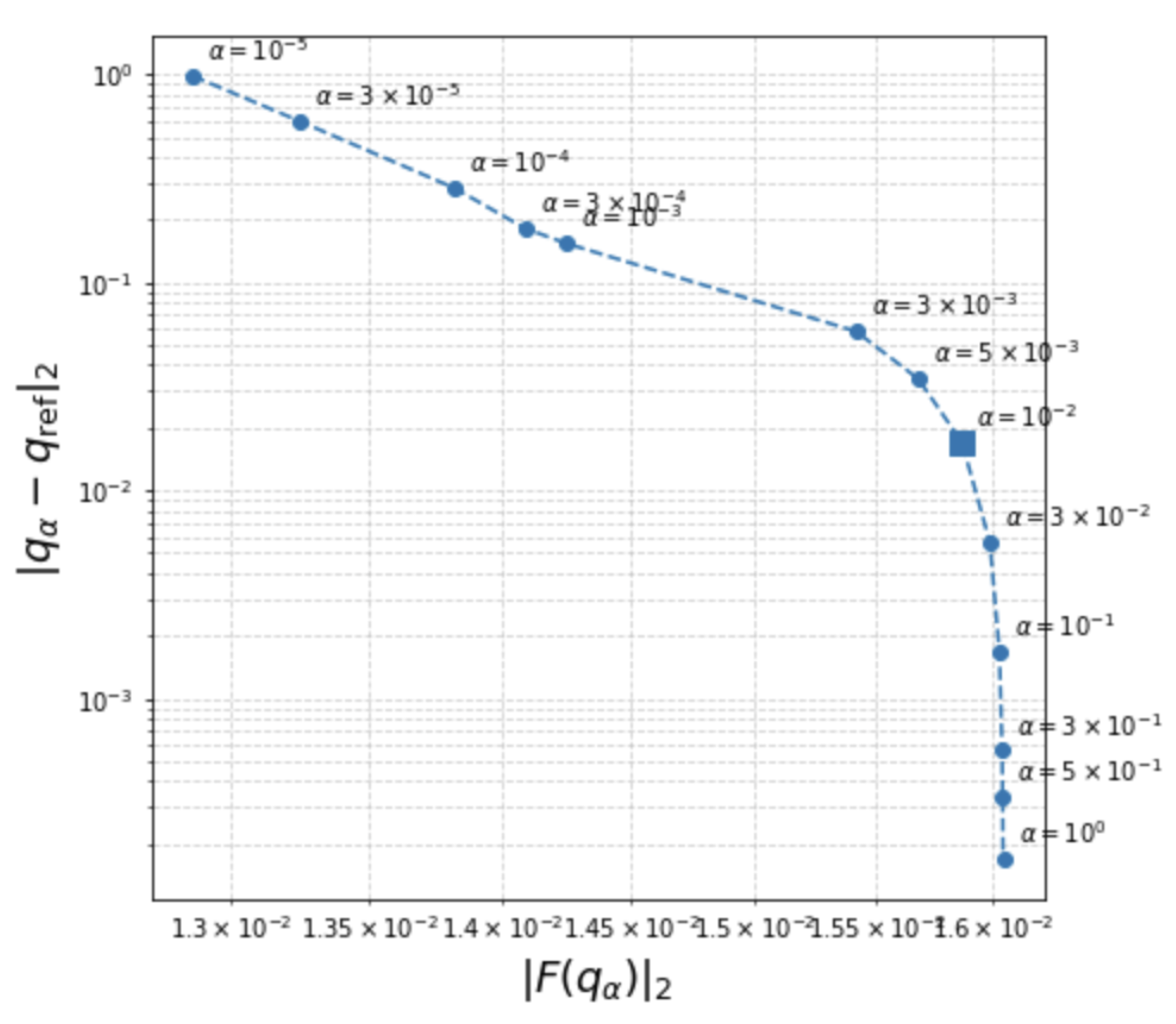
The regularization parameter $\alpha$ is selected using the L-curve criterion. The L-curve represents the trade-off between the data misfit norm $\parallel F\left(q_{\alpha }\right){\parallel }_2$ and the regularization norm $\parallel q_{\alpha }-q_{\mathrm{ref}}{\parallel }_2$.

As shown in Figure 9, the L-curve exhibits a smooth transition rather than a sharp corner, which is typical for moderately well-posed inverse problems. The value $\alpha ={10}^{-2}$ is chosen as it lies in the transition region, providing a balance between the data misfit and the deviation from the reference parameters.

Tikhonov regularization is incorporated into the formulation to improve the stability of the parameter estimation [21,43,44,45].

The inverse problem remains sensitive to measurement noise and modeling uncertainties, particularly due to the use of truncated Fourier expansions and limited experimental information in the angular direction.

The results presented in

Table 2. Dependence of reconstructed parameters on the regularization parameter.

$\mathit{\alpha }$	${\mathit{k}}_1$	${\mathit{k}}_2$	${\mathit{k}}_3$	h	$\mathit{Bi}$
${10}^{-3}$	0.332	0.606	0.704	5.501	2.10
${10}^{-2}$	0.334	0.608	0.705	5.501	2.11
${10}^{-1}$	0.336	0.609	0.706	5.500	2.11

demonstrate that the reconstructed parameters exhibit only weak dependence on the regularization parameter within a broad range of values. This indicates that the inverse problem is not severely ill-posed and that the solution remains stable with respect to variations of $\alpha$. In this case, regularization primarily serves to control parameter variability rather than to suppress instability.

To ensure physically meaningful solutions, the following bounds are imposed:

$$k_s\in [0.2,2.0]{\displaystyle \frac{\mathrm{W}}{\mathrm{m}·\mathrm{K}}},s=1,2,3,h\in [1,20]{\displaystyle \frac{\mathrm{W}}{{\mathrm{m}}^2\mathrm{K}}}.$$

These ranges correspond to typical thermophysical properties of soils and convective heat transfer conditions [34,36].

Thus, the inverse problem is reduced to a constrained regularized optimization problem combining analytical modeling, Fourier decomposition, and experimental data.

5.2. Residual Vector and Least Squares Functional

The components of the data misfit functional introduced in the previous subsection are defined as follows. To establish the connection between the analytical model and the experimental data, the temperature distributions at the interfaces are projected onto the Fourier basis. This allows transforming the inverse problem into a comparison between the Fourier coefficients obtained from the analytical solution and those reconstructed from the temperature data. Such an approach reduces the influence of measurement noise and enables a consistent identification of the thermophysical parameters. For each harmonic $n\ge 1$, a residual vector is introduced to quantify the discrepancy between the model-based and experimentally obtained Fourier coefficients at the interfaces $r=r_2$ and $r=r_3$:

$$F_n\left(\mathbf{q}\right)=\left(\begin{array}{c}{a}_{n,\mathrm{mod}}^{\left(2\right)}\left(\mathbf{q}\right)-a_{n,\exp }^{\left(2\right)}\\ b_{n,\mathrm{mod}}^{\left(2\right)}\left(\mathbf{q}\right)-b_{n,\exp }^{\left(2\right)}\\ a_{n,\mathrm{mod}}^{\left(3\right)}\left(\mathbf{q}\right)-a_{n,\exp }^{\left(3\right)}\\ b_{n,\mathrm{mod}}^{\left(3\right)}\left(\mathbf{q}\right)-b_{n,\exp }^{\left(3\right)}\end{array}\right),$$

(34)

where $\mathbf{q}={(k_1,k_2,k_3,h)}^T$ is the vector of unknown parameters.

The model-based coefficients are obtained from the analytical solution:

$$a_{n,\mathrm{mod}}^{\left(2\right)}=A_n^{\left(2\right)}{r}_2^n+A_{-n}^{\left(2\right)}{r}_2^{-n},b_{n,\mathrm{mod}}^{\left(2\right)}=B_n^{\left(2\right)}{r}_2^n+B_{-n}^{\left(2\right)}{r}_2^{-n},$$

(35)

$$a_{n,\mathrm{mod}}^{\left(3\right)}=A_n^{\left(3\right)}{r}_3^n+A_{-n}^{\left(3\right)}{r}_3^{-n},b_{n,\mathrm{mod}}^{\left(3\right)}=B_n^{\left(3\right)}{r}_3^n+B_{-n}^{\left(3\right)}{r}_3^{-n}.$$

(36)

The experimental Fourier coefficients are computed as

$$a_{n,\exp }^{\left(s\right)}={\displaystyle \frac{1}{\pi }}{\int }_0^{2\pi }{T}^{\left(s\right)}(r_s,\phi )cos\left(n\phi \right)d\phi ,b_{n,\exp }^{\left(s\right)}={\displaystyle \frac{1}{\pi }}{\int }_0^{2\pi }{T}^{\left(s\right)}(r_s,\phi )sin\left(n\phi \right)d\phi .$$

(37)

For the zeroth harmonic:

$$F_0\left(\mathbf{q}\right)=\left(\begin{array}{c}{\overline{T}}_{\mathrm{mod}}^{\left(2\right)}-{\overline{T}}_{\exp }^{\left(2\right)}\\ {\overline{T}}_{\mathrm{mod}}^{\left(3\right)}-{\overline{T}}_{\exp }^{\left(3\right)}\end{array}\right),$$

(38)

where ${\overline{T}}_{\exp }^{\left(s\right)}={\displaystyle \frac{1}{2\pi }}{\int }_0^{2\pi }{T}^{\left(s\right)}(r_s,\phi )d\phi ,$ $s=2,3$.

The data misfit functional is defined as:

$$J_{\mathrm{data}}\left(\mathbf{q}\right)={\displaystyle \frac{1}{2}}\parallel F_0{\left(\mathbf{q}\right)\parallel }_2^2+{\displaystyle \frac{1}{2}}{\displaystyle \sum _{n=1}^N}{\parallel F_n\left(\mathbf{q}\right)\parallel }_2^2.$$

(39)

5.3. Projected Gradient-Based Minimization with Constraints

The minimization of the functional $J\left(\mathbf{q}\right)$ is performed using a first-order gradient-based method. Taking into account physical constraints imposed on the unknown parameters, the problem is formulated as a constrained optimization problem over the admissible set

$$\mathrm{\Omega }=\left\{\mathbf{q}:k_s>0,h>0,s=1,2,3\right\}.$$

In this setting, a projected gradient method is employed, where the iterative scheme is given by

$${\mathbf{q}}^{(i+1)}={\mathrm{\Pi }}_{\mathrm{\Omega }}\left({\mathbf{q}}^{\left(i\right)}-{\gamma }_i\nabla J\left({\mathbf{q}}^{\left(i\right)}\right)\right),$$

(40)

where ${\gamma }_i>0$ denotes the step size, and ${\mathrm{\Pi }}_{\mathrm{\Omega }}$ is the operator of orthogonal projection onto the set $\mathrm{\Omega }$.

Substituting the expression for the gradient of the functional yields the following iterative scheme:

$${\mathbf{q}}^{(i+1)}={\mathrm{\Pi }}_{\mathrm{\Omega }}\left[{\mathbf{q}}^{\left(i\right)}-{\gamma }_i\left(\mathcal{J}{\left({\mathbf{q}}^{\left(i\right)}\right)}^T\mathcal{F}\left({\mathbf{q}}^{\left(i\right)}\right)+\alpha ({\mathbf{q}}^{\left(i\right)}-{\mathbf{q}}_{\mathrm{ref}})\right)\right].$$

(41)

The use of the projection operator ensures that the physical constraints on the parameters are satisfied at each iteration of the algorithm and prevents the occurrence of non-physical values of the thermal conductivity and heat transfer coefficient.

In practical implementation, the projection ${\mathrm{\Pi }}_{\mathrm{\Omega }}$ is performed component-wise by mapping parameter values that fall outside the admissible set onto the boundary of $\mathrm{\Omega }$.

The practical implementation of the algorithm consists of the following steps:

Step 1. Initialization with the initial guess ${\mathbf{q}}^{\left(0\right)}={\mathbf{q}}_{\mathrm{apr}}$.

Step 2. Evaluation of the parameters $k_1,k_2,k_3,h$.

Step 3. Solution of the direct problem for each harmonic and construction of the residual vectors $F_n\left({\mathbf{q}}^{\left(i\right)}\right)$.

Step 4. Computation of the functional value $J\left({\mathbf{q}}^{\left(i\right)}\right)$ and its gradient $\nabla J\left({\mathbf{q}}^{\left(i\right)}\right)$.

Step 5. Execution of the projected gradient descent step:

$${\mathbf{q}}^{(i+1)}={\mathrm{\Pi }}_{\mathrm{\Omega }}\left({\mathbf{q}}^{\left(i\right)}-{\gamma }_i\nabla J\left({\mathbf{q}}^{\left(i\right)}\right)\right).$$

Step 6. Stopping criterion:

$$\parallel {\mathbf{q}}^{(i+1)}-{\mathbf{q}}^{\left(i\right)}{\parallel }_2<\epsilon \mathrm{or}{\parallel \nabla J\left({\mathbf{q}}^{\left(i\right)}\right)\parallel }_2<\epsilon .$$

(42)

The tolerance parameter $\epsilon$ was chosen of the order of ${10}^{-6}$, which ensured stable convergence of the solution [46].

Thus, the proposed algorithm ensures stable and physically consistent parameter identification through the combined use of Tikhonov regularization and the projected gradient method.

5.4. Numerical Solution and Results Analysis

The numerical solution of the inverse problem was carried out using the truncated Fourier expansion with harmonics $n=0,1,\dots ,15$. The number of harmonics is chosen to represent the temperature field while limiting the influence of high-frequency components.

The thermophysical parameters $k_1$, $k_2$, $k_3$, and h are treated as constants independent of the harmonic number. The reconstruction results demonstrate that the proposed inverse procedure yields stable and physically meaningful values of the parameters.

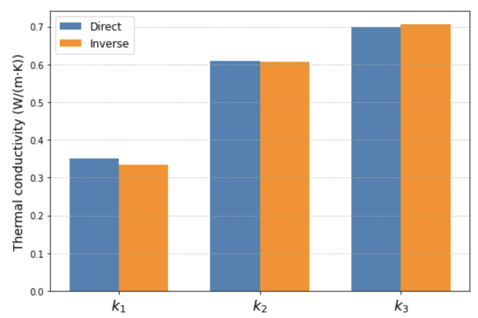
Figure 10 shows the comparison between the reconstructed thermal conductivities and the corresponding reference values. A good agreement between the reconstructed and reference values is observed for all three layers. The relative error does not exceed a few percent, indicating that the inverse method accurately captures the thermal properties of the multilayer system.

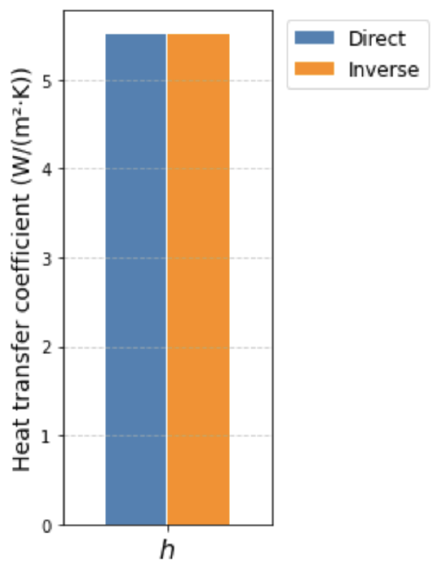
Figure 11 presents the comparison for the heat transfer coefficient. The reconstructed value is in excellent agreement with the reference one, with a negligible relative error. This result is consistent with the adopted modeling assumptions.

For a quantitative assessment of the reconstruction accuracy,

Table 3. Comparison of reference and reconstructed thermophysical parameters.

Parameter	Direct Problem	Inverse Problem	Unit	Absolute Error	Relative Error (%)
$k_1$	0.350000	0.334082	W m−1 K−1	0.015918	4.547951
$k_2$	0.610000	0.607543	W m−1 K−1	0.002457	0.402801
$k_3$	0.700000	0.705420	W m−1 K−1	0.005420	0.774257
h	5.500000	5.500543	W m−1 K−1	0.000543	0.009875
$Bi$	2.121429	2.105337	-	0.016091	0.758509

presents the comparison between the reference (direct problem) and reconstructed (inverse problem) thermophysical parameters.

As shown in Table 3, the reconstructed thermophysical parameters are in very good agreement with the reference values obtained from the direct problem.

The relative errors for $k_2$ and $k_3$ do not exceed $1\%$, indicating high accuracy of the reconstruction for the middle and outer layers. The heat transfer coefficient h is recovered with extremely high precision, with a relative error below $0.01\%$, which confirms the correctness of the boundary heat exchange modeling.

The largest deviation is observed for the thermal conductivity $k_1$ of the inner layer, where the relative error is approximately $4.55\%$. This can be explained by the lower sensitivity of the temperature field to the properties of the innermost region, as well as by the limited influence of the inner boundary on the external measurement data.

Overall, the obtained results indicate that the inverse method yields accurate and physically consistent estimates of the thermophysical parameters. The inclusion of Tikhonov regularization improves the stability of the solution without introducing significant bias into the reconstructed values.

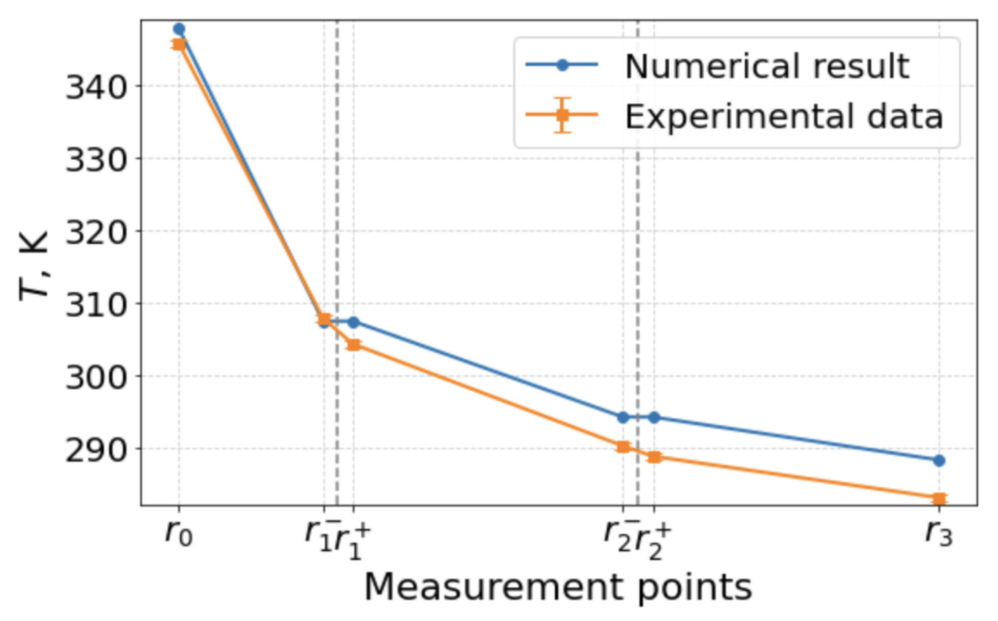
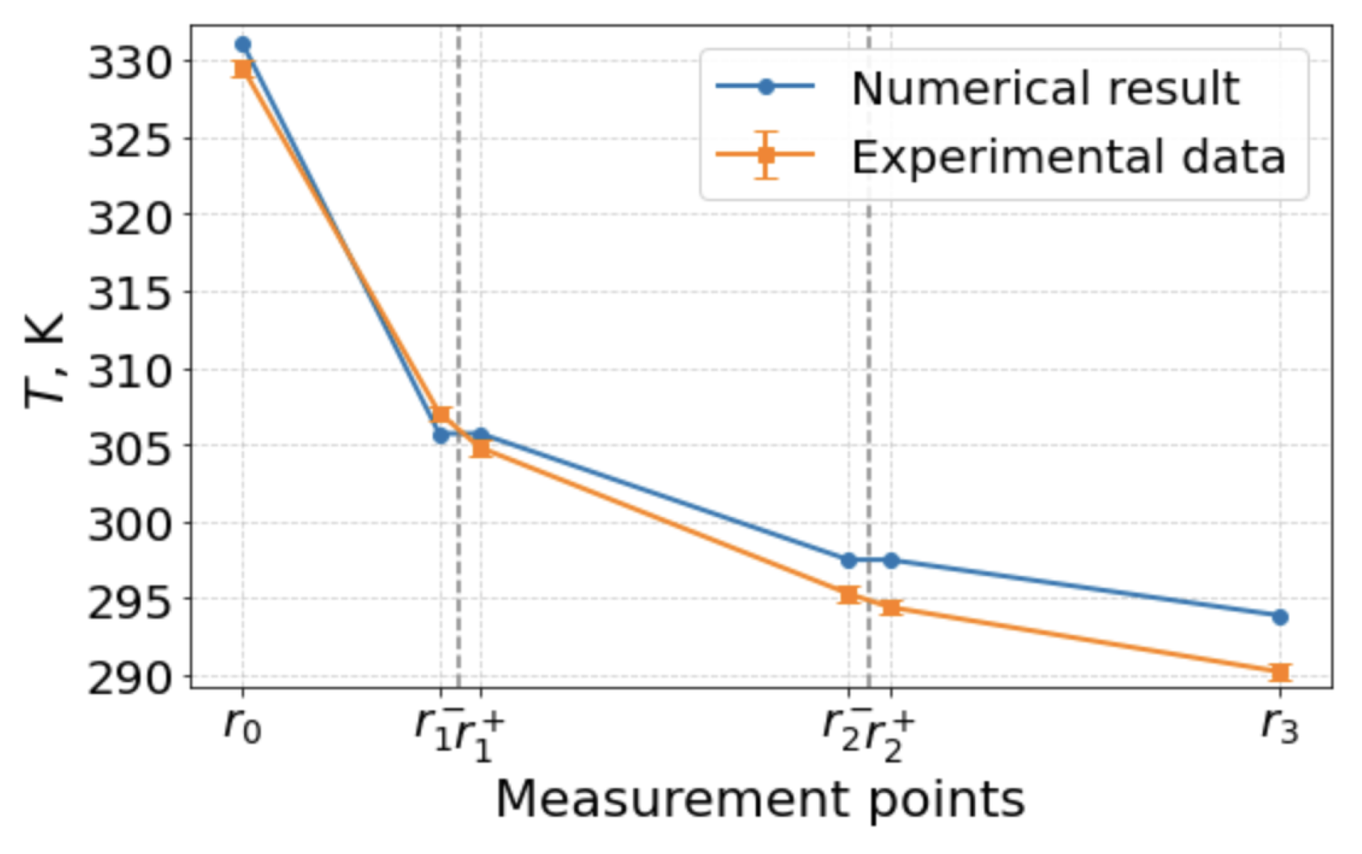
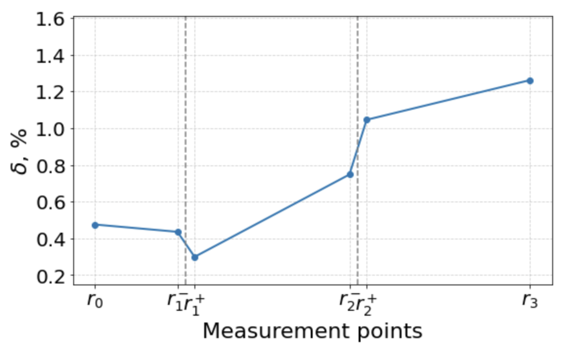
To validate the robustness of the proposed inverse method, additional numerical experiments were carried out for different time instants corresponding to the 4th, 12th, and 138th days of the experiment. For each case, the temperature distribution obtained using the reconstructed parameters was compared with the corresponding experimental data.

The validation calculations were performed using experimental data corresponding to different days and time instants of the observation period. The initial reference date (day 1) corresponds to November 2. The ambient air temperatures used as input data are summarized in

Table 4. Input data used for validation calculations.

Day	Date	Time	${\mathit{T}}_{\mathit{a}}$ (K)
4	5 November	04:00	285.03
12	13 November	15:00	282.12
138	19 March	13:40	290.02

.

The comparison results demonstrate consistently good agreement between the numerical solution and the experimental measurements for all considered days. The relative error remains below approximately $2\%$ for all measurement points in Figure 12, Figure 13 and Figure 14, confirming the stability of the reconstruction under varying thermal conditions.

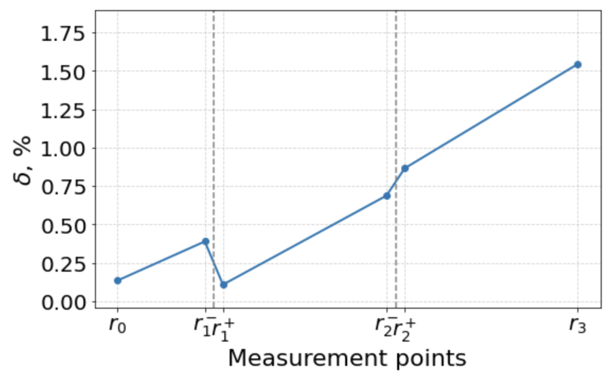
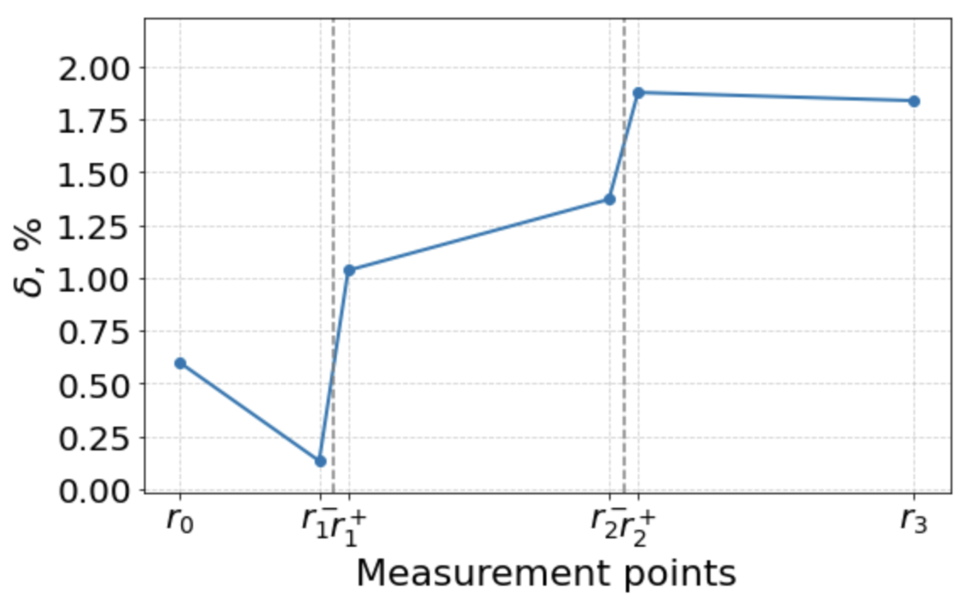
The distribution of the relative error along the measurement points for the considered cases is presented in Figure 15, Figure 16 and Figure 17. It can be observed that the error remains low across all regions of the domain, with slightly larger deviations near the outer boundary, which is typical for inverse heat conduction problems.

For a quantitative assessment of the reconstruction accuracy,

Table 5. Summary of reconstruction accuracy for different days.

Day	Mean Error (%)	Maximum Error (%)
4	0.62	1.54
12	1.14	1.88
138	0.71	1.26

summarizes the mean and maximum relative errors for each considered case.

The presented results confirm that the reconstructed parameters remain stable and provide accurate predictions for different experimental conditions. The use of Tikhonov regularization ensures robustness of the inverse solution and suppresses the influence of measurement noise.

Thus, the proposed approach, combining analytical modeling, Fourier decomposition, least-squares minimization, and regularization, provides an effective and reliable tool for solving inverse heat conduction problems in multilayer cylindrical systems.

6. Conclusions

In this study, a comprehensive analysis of steady-state heat transfer in a three-layer cylindrical system with angular inhomogeneity of the temperature field has been carried out. A mathematical model in cylindrical coordinates was developed, taking into account piecewise-constant thermophysical properties of the layers and convective heat exchange at the outer boundary.

An analytical solution of the direct problem was obtained using a Fourier series expansion with respect to the angular coordinate. This approach ensures an accurate representation of the temperature field and proper enforcement of the interface conditions between the layers. The numerical results confirm the stability and physical consistency of the direct problem solution.

Based on experimental temperature measurements, an inverse problem for the reconstruction of the thermal conductivities of the layers and the heat transfer coefficient was formulated and solved. The thermophysical parameters were treated as constants independent of the harmonic number, ensuring physical consistency of the model.

The inverse problem was solved using a nonlinear least-squares formulation with Tikhonov regularization. The inclusion of the regularization term improves the stability of the solution and reduces sensitivity to measurement noise and modeling uncertainties. The reconstructed parameters show very good agreement with the reference values, with relative errors below approximately $5\%$, and significantly smaller errors for most parameters.

To assess the robustness of the proposed approach, additional validation was performed using temperature data corresponding to different days and time instants of the experiment. The results demonstrate that the reconstructed parameters provide accurate predictions under varying thermal conditions. The relative error between the numerical and experimental temperature distributions remains below approximately $2\%$ for all considered cases.

The results indicate that the inverse method yields reliable and physically consistent estimates of the thermophysical parameters in multilayer cylindrical systems. The combination of analytical modeling, Fourier decomposition, least-squares minimization, and regularization ensures both accuracy and stability of the solution.

The proposed approach can be applied to a wide range of engineering problems, including thermal analysis of soils, underground structures, and multilayer insulation systems.

Future research may include the extension of the method to transient heat conduction problems, as well as the incorporation of anisotropic properties and nonlinear heat transfer effects.