Accountability-Aware Fractional Control for Embodied Intelligent Systems: Mittag-Leffler Stability and Conditional Proxemic Safety

Abstract

This paper develops an accountability-aware fractional control framework for embodied intelligent systems in shared human environments. The approach combines a Caputo fractional-order stabilizing law, an intent-evidence realization with softmax belief reconstruction, and a conditional proxemic safety layer. Sufficient conditions are established for local Mittag-Leffler stability of the augmented error dynamics and forward invariance of the safe set. Numerical results are presented as a theorem-validation benchmark. For the base case with $\alpha =0.9$, the augmented error norm decays from $1.2359$ to $9.90\times {10}^{-3}$ while the safety margin remains strictly positive, and the robustness condition is satisfied with a margin of $1.8641$. An $\alpha$-sweep and a step-size convergence study further show that the fractional order induces a systematic safety–performance trade-off and that the reported behaviors are numerically stable. Additional simulations with four intent classes, bounded observation noise, and Monte Carlo uncertainty stress tests are included to strengthen the numerical evidence beyond the two-intent theorem-validation case. The manuscript also clarifies the quantitative interpretation of the accountability index, the conditional nature of the safety theorem, and an implementable sampled safety-filter realization for concrete robotic platforms. The results support the proposed framework as a mathematically consistent tool for shaping the balance between regulation and proxemic safety.

1. Introduction

Autonomous embodied intelligent systems are increasingly required to operate in human environments such as homes, hospitals, offices, and public spaces, in which the ability to be autonomous means more than the ability to move without collisions and achieve a goal. In these environments, robots need to operate safely, express their intentions through actions, and adhere to interaction norms that ensure that their actions are understandable and acceptable to human bystanders. Such a view has driven much of the recent research on human-aware and socially aware robot navigation, which focuses on comfort, coordination, and interaction quality, as well as geometric and dynamic safety [1,2,3]. Meanwhile, proxemics is still an important concept for socially acceptable robot behavior, as interpersonal distance, spatial alignment, and context-dependent “bubbles” of personal space have a strong influence on the way robot movement is perceived in social spaces [4,5,6].

This issue is even more critical when robots are used as assistive, service, or collaborative robots, whose motion is perceived not only as physical motion but also as a means of communication about future action, intentions, and interaction. This is especially important in socially assistive robotics and other HRI applications, where users learn about the robot’s next actions and the trustworthiness, cooperativeness, and adherence to norms of the motion from visual observation [7,8,9]. More recent research has also found that legibility is best achieved when intent is communicated at the interaction level (for example, passing side or yielding), as well as the destination level, and that such communication is also influenced by human attention [1]. Meanwhile, recent surveys and benchmarks have identified the need for navigation approaches that address safety, social acceptability, and realistic evaluation in the context of crowd dynamics and variability [10,11,12].

One of the challenges in realizing this vision is that the goal of accountability-aware robot behavior relates to latent and observer-specific interaction variables such as inferred intent, predictability, comfort, and social norms. As a result, state-of-the-art human–robot interaction increasingly makes use of belief-state reasoning, recursive intent inference, and multimodal perception-based decision making. Bayesian intent estimation and belief update have been long thought to be natural models for shared-control robotics and assistance [13,14]. This view has been broadened by recent work on multimodal HRI using vision, motion, language, and other context signals for decision making and influencing interactions [14,15]. Similarly, knowledge of human intent is explicitly used to resolve robot actions, enable smooth interaction, and maintain human control in intent-aware shared-control and collaborative manipulation [16,17,18].

From a control-theoretic perspective, however, it can be challenging to ensure both interaction-sensitive regulation and safety, particularly when the robot behavior needs to be based on temporally extended, rather than instantaneous, cues. Here, fractional-order dynamics are an attractive option because they embody memory, history dependence, and long-range temporal interactions, which are all important for embodied interaction and intention communication. Fractional differential equations, Caputo derivatives, and Mittag-Leffler functions are all now well understood, and they have been well studied as mathematically rigorous representations of systems with nonlocal temporal dynamics [19,20,21]. For linear fractional-order systems, the sectorial stability characterization due to Matignon plays the role of the Hurwitz criterion [22], and for nonlinear systems, the notions of the Lyapunov direct method and the generalized Mittag-Leffler stability are well accepted [23,24,25]. It has been shown recently that Lyapunov methods need to be refined for Caputo systems, the role of comparative principles has been clarified, and stability results have been extended to systems with delays, impulsive effects, and structured nonlinearities for fractional order [26,27,28]. Moreover, generalized Grönwall inequalities and fractional comparison arguments continue to be key analytical tools for proving well-posedness and convergence estimates [29,30,31].

Despite these advances, human-aware navigation and accountability-aware interaction combined with fractional-order control are still relatively unexplored. Most current fractional-order control works highlight stability, synchronization, or robustness in abstract systems, while most social navigation works focus on planning, learning or user studies without providing rigorous fractional-order closed-loop guarantees. This is particularly the case in the safety layer. Barrier-function methods have emerged as a powerful way to ensure forward invariance (and safety) in integer-order systems, but their adoption to Caputo fractional-order systems is more recent and evolving [32,33]. Even these recent advances primarily consider generic fractional nonlinear systems rather than embodied intelligent systems with safety co-existing with intent revelation, interpretability and human-aware regulation. So there is a need for a comprehensive approach that integrates fractional-order stability analysis, conditional safety and accountably-aware interaction goals in a mathematical framework.

A parallel and equally important issue concerns transparency and explanation. As robots enter socially sensitive environments, it is no longer sufficient that they act correctly; they must also be able to justify, communicate, or at least embody their decision rationale in a form that humans can interpret. This requirement has motivated recent work on explainable robot navigation and hierarchical explanation frameworks for autonomous motion, particularly in settings where robot behavior affects trust, comfort, and perceived competence [34,35]. However, explainability in navigation is often treated separately from low-level closed-loop control and separately again from formal safety guarantees. In contrast, the present work adopts an operational view of accountability: the robot should generate motion and internal evidence dynamics that are not only stable and safe, but they are also measurable and interpretable through accountability-related outputs such as proxemic compliance, intent confidence, predictability, and rule consistency.

Motivated by these observations, this paper develops an accountability-aware fractional control framework for embodied intelligent systems. The proposed approach combines a fractional-order control law with an internal intent-evidence state, a softmax-based belief realization, and a conditional proxemic safety layer. Rather than interpretability being an ex-post criterion for evaluation, we include accountability-related measures into the regulated output and obtain a closed-loop error dynamics model that can be subject to rigorous fractional Lyapunov analysis. We employ Caputo-compatible quadratic estimates and comparison theorems, to establish Mittag-Leffler-type convergence for the error dynamics [24,25,26]. We embed safety via a fractional barrier inequality directly on the proxemic margin, without any invalid application of an unrealisable classical chain rule for Caputo derivatives and in line with contemporary barrier-based fractional analysis [30,32,33].

The main contributions of this work are as follows:

• We formulate a proxemic safety-preserving accountability-aware control problem for embodied intelligent systems that integrates task tracking, proxemic safety, and interaction-level interpretability through a composite regulated output with an explicit quantitative accountability interpretation.
• We introduce a finite-dimensional intent-evidence realization with softmax belief reconstruction, embedding observer-dependent legibility and accountability quantities into an augmented fractional-order state representation suitable for feedback design and analysis.
• We design a nominal accountability-aware controller and establish local Mittag-Leffler stability of the embedded error dynamics using a Caputo-compatible quadratic Lyapunov estimate and an explicit robustness margin condition.
• We present a conditional proxemic safety layer based on a fractional barrier inequality and add a sampled optimization-based realization that can synthesize or verify the auxiliary safety correction for a concrete discretized robot model.
• We strengthen the numerical validation by adding an integer-order baseline, an $\alpha$-sweep, a step-size study, a four-intent noisy benchmark, and Monte Carlo uncertainty tests, while clearly separating theorem-validation evidence from future real-robot experimental validation.

The paper is organized as follows. Section 2 reviews the required tools from fractional calculus, Caputo stability theory, and embodied interaction. Section 3 defines the accountability-aware control problem and introduces the relevant safety, legibility, predictability, and accountability quantities. Section 4 presents the control-oriented augmented model, the nominal stabilizing law, the conditional safety layer, and the main closed-loop theorems. The simulation section then validates the theoretical results numerically in a theorem-aligned benchmark representative of accountability-aware embodied control.

2. Preliminaries

This section recalls the main tools from fractional calculus and human-aware embodied interaction that are needed in the sequel. We focus on Caputo fractional-order models with order $\alpha \in (0,1)$, since they are particularly suitable for control design with standard initial conditions and admit a convenient Volterra integral representation [19,20,21]. Moreover, because the present work concerns embodied intelligent systems operating in human-populated environments, we also recall the notions of proxemics, legibility, predictability, and operational accountability that will later be incorporated into the control design [1,4,7,8,9].

Fractional-order dynamics are adopted here not as a mere generalization of integer-order models, but as a principled framework for representing fading-memory and nonlocal temporal effects that naturally arise in embodied systems and in human-aware interaction processes. In particular, accountability-aware behavior depends not only on instantaneous geometry but also on recent motion history, intent revelation, and temporally extended interaction cues. This makes fractional-order models and controllers a natural candidate for shaping both closed-loop stability and interaction quality [1,20,25].

2.1. Notation

Let ${\mathbb{R}}^n$ denote the n-dimensional Euclidean space and let $∥·∥$ denote the Euclidean norm. For a matrix $A\in {\mathbb{R}}^{n\times n}$, $\sigma \left(A\right)$ denotes its spectrum, and ${\lambda }_i\left(A\right)$ denotes its ith eigenvalue. The identity matrix of dimension n is denoted by $I_n$.

For a continuous signal $z:[0,T]\to {\mathbb{R}}^n$, we denote by $z_{[0,t]}$ its history on $[0,t]$. A continuous function ${\alpha }_1:{\mathbb{R}}_{\ge 0}\to {\mathbb{R}}_{\ge 0}$ is said to belong to class $\mathcal{K}$ if it is strictly increasing and ${\alpha }_1\left(0\right)=0$. It belongs to class ${\mathcal{K}}_{\infty }$ if, in addition, ${\alpha }_1\left(r\right)\to \infty$ as $r\to \infty$. A continuous function $\beta :{\mathbb{R}}_{\ge 0}\times {\mathbb{R}}_{\ge 0}\to {\mathbb{R}}_{\ge 0}$ is of class $\mathcal{KL}$ if $\beta (·,s)\in \mathcal{K}$ for each fixed $s\ge 0$, and $\beta (r,·)$ decreases to zero for each fixed $r\ge 0$.

2.2. Fractional Integral, Caputo Derivative, and Mittag-Leffler Functions

We first recall the standard fractional operators and special functions used throughout the paper [19,20,21].

Definition 1 (Gamma function).

For $z>0$, the Gamma function is defined by

$$\mathsf{\Gamma }\left(z\right)={\int }_0^{\infty }{t}^{z-1}{e}^{-t}dt.$$

(1)

Definition 2 (Riemann–Liouville fractional integral).

Let $\alpha >0$ and let $f:[0,T]\to {\mathbb{R}}^n$ be locally integrable. The left-sided Riemann–Liouville fractional integral of order α is defined by

$$\left(I^{\alpha }f\right)\left(t\right)={\displaystyle \frac{1}{\mathsf{\Gamma }\left(\alpha \right)}}{\int }_0^t{(t-\tau )}^{\alpha -1}f\left(\tau \right)d\tau ,t\in [0,T].$$

(2)

Definition 3 (Caputo fractional derivative).

Let $\alpha \in (0,1)$ and let $f:[0,T]\to {\mathbb{R}}^n$ be absolutely continuous. The Caputo fractional derivative of order α is defined by

$$\left({}^{C}D_t^{\alpha }f\right)\left(t\right)={\displaystyle \frac{1}{\mathsf{\Gamma }(1-\alpha )}}{\int }_0^t{(t-\tau )}^{-\alpha }\dot{f}\left(\tau \right)d\tau ,t\in [0,T].$$

(3)

Remark 1.

The Caputo derivative is especially convenient in engineering applications because it allows the use of standard initial conditions such as $x\left(0\right)=x_0$, in contrast with the Riemann–Liouville derivative, which typically requires fractional initial data [19,20].

Definition 4 (Mittag-Leffler functions).

For $\alpha >0$ and $\beta >0$, the two-parameter Mittag-Leffler function is defined by

$$E_{\alpha ,\beta }\left(z\right)={\displaystyle \sum _{k=0}^{\infty }}{\displaystyle \frac{z^k}{\mathsf{\Gamma }(\alpha k+\beta )}},z\in \mathbb{C}.$$

(4)

The one-parameter Mittag-Leffler function is obtained as

$$E_{\alpha }\left(z\right)=E_{\alpha ,1}\left(z\right)={\displaystyle \sum _{k=0}^{\infty }}{\displaystyle \frac{z^k}{\mathsf{\Gamma }(\alpha k+1)}}.$$

(5)

Remark 2.

The Mittag-Leffler function plays, for fractional-order systems, a role analogous to the exponential function for integer-order systems. Indeed, $E_1\left(z\right)=e^z$, and many stable fractional-order dynamics decay according to expressions of the form $E_{\alpha }(-c{t}^{\alpha })$ [19,23,24].

2.3. Integral Representation and Well-Posedness

The following result is standard and will be repeatedly used to transform a Caputo differential equation into an equivalent Volterra integral equation with weakly singular kernel [20,21].

Lemma 1 (Volterra integral representation).

Consider the Caputo fractional differential equation

$${}^{C}D_t^{\alpha }x\left(t\right)=F(t,x\left(t\right)),x\left(0\right)=x_0,$$

(6)

where $\alpha \in (0,1)$ and $F:[0,T]\times {\mathbb{R}}^n\to {\mathbb{R}}^n$ is continuous. In the standard solution class for Caputo initial-value problems, (6) is equivalent to

$$x\left(t\right)=x_0+{\displaystyle \frac{1}{\mathsf{\Gamma }\left(\alpha \right)}}{\int }_0^t{(t-\tau )}^{\alpha -1}F(\tau ,x\left(\tau \right))d\tau ,t\in [0,T].$$

(7)

Remark 3.

Lemma 1 is understood in the usual sense of Caputo initial-value theory: if x satisfies (6) almost everywhere, then it satisfies (7) for all t, and conversely, a solution of (7) belongs to the standard regularity class used in the analysis of Caputo problems [20].

Assumption 1 (Regularity of the vector field).

Unless otherwise stated, the vector field $F(t,x)$ is assumed to be continuous in t and locally Lipschitz in x on compact subsets of $[0,T]\times {\mathbb{R}}^n$.

Proposition 1 (Existence and uniqueness).

Under Assumption 1, for every initial condition $x_0\in {\mathbb{R}}^n$, the Caputo system (6) admits a unique local solution. If, in addition, F satisfies a linear growth condition, then the solution exists on the whole interval $[0,T]$ [20,21].

For linear systems, the solution can be written explicitly using matrix Mittag-Leffler functions.

Proposition 2 (Solution of a linear Caputo system).

Consider

$${}^{C}D_t^{\alpha }x\left(t\right)=Ax\left(t\right)+\phi \left(t\right),x\left(0\right)=x_0,$$

(8)

where $\alpha \in (0,1)$, $A\in {\mathbb{R}}^{n\times n}$, and $\phi :[0,T]\to {\mathbb{R}}^n$ is continuous. Then the unique solution is

$$x\left(t\right)=E_{\alpha }\left(A{t}^{\alpha }\right)x_0+{\int }_0^t{(t-\tau )}^{\alpha -1}{E}_{\alpha ,\alpha }\left(A{(t-\tau )}^{\alpha }\right)\phi \left(\tau \right)d\tau .$$

(9)

Remark 4.

Proposition 2 will later be useful for deriving nominal closed-loop solutions, perturbation bounds, and comparison estimates for the accountability-aware controlled dynamics [19,20].

2.4. Useful Inequalities and Stability Notions

The next inequality is a fractional counterpart of the classical Grönwall lemma and is fundamental for deriving robustness and convergence bounds [29].

Lemma 2 (Generalized fractional Grönwall inequality).

Let $u:[0,T]\to {\mathbb{R}}_{\ge 0}$ be locally integrable and suppose that

$$u\left(t\right)\le a\left(t\right)+b{\int }_0^t{(t-\tau )}^{\alpha -1}u\left(\tau \right)d\tau ,t\in [0,T],$$

(10)

where $\alpha \in (0,1)$, $b\ge 0$ is constant, and $a:[0,T]\to {\mathbb{R}}_{\ge 0}$ is nonnegative and nondecreasing. Then

$$u\left(t\right)\le a\left(t\right)E_{\alpha }\left(b\mathsf{\Gamma }\left(\alpha \right)t^{\alpha }\right),t\in [0,T].$$

(11)

For linear autonomous fractional-order systems, asymptotic stability is characterized by the celebrated Matignon criterion [22].

Proposition 3 (Matignon stability criterion).

Consider the linear fractional-order system

$${}^{C}D_t^{\alpha }x\left(t\right)=Ax\left(t\right),\alpha \in (0,1).$$

(12)

The equilibrium $x=0$ is asymptotically stable if and only if

$$\left|\arg \left({\lambda }_i\left(A\right)\right)\right|>{\displaystyle \frac{\alpha \pi }{2}},\forall {\lambda }_i\left(A\right)\in \sigma \left(A\right).$$

(13)

Remark 5.

Proposition 3 reduces to the classical Hurwitz condition when $\alpha =1$. For $\alpha \in (0,1)$, the stability region becomes a sector of the complex plane, which is a fundamental feature of fractional-order systems [22].

The following stability notion is particularly suitable for nonlinear fractional-order systems.

Definition 5 (Mittag-Leffler stability).

Consider the nonlinear Caputo system

$${}^{C}D_t^{\alpha }x\left(t\right)=F\left(x\left(t\right)\right),F\left(0\right)=0,\alpha \in (0,1).$$

(14)

The equilibrium $x=0$ is said to be Mittag-Leffler stable if there exist constants $c>0$, $d>0$, and $\rho >0$ such that, for all sufficiently small initial conditions,

$$∥x\left(t\right)∥\le {\left\{d{E}_{\alpha }(-c{t}^{\alpha })\right\}}^{\rho },\forall t\ge 0.$$

(15)

Lemma 3 (Quadratic Caputo derivative estimate).

Let $e:[0,T]\to {\mathbb{R}}^n$ be a real solution of a Caputo fractional-order system with $\alpha \in (0,1)$, and let $P=P^{\top }\succ 0$. Then, under the regularity assumptions ensuring that the quantities below are well defined,

$${}^{C}D_t^{\alpha }\left(e^{\top }\left(t\right)Pe\left(t\right)\right)\le e^{\top }\left(t\right)P{}^{C}D_t^{\alpha }e\left(t\right)+{\left({}^{C}D_t^{\alpha }e\left(t\right)\right)}^{\top }Pe\left(t\right).$$

(16)

Remark 6.

Lemma 3 is the appropriate substitute for the unavailable classical chain rule in Caputo systems. In the main results, whenever quadratic Lyapunov functions are used, the analysis will rely on Lemma 3 and on comparison arguments, rather than on a formal classical differentiation of a composition [25,26,27].

Proposition 4 (Comparison-based sufficient condition for Mittag-Leffler stability).

Let $\alpha \in (0,1)$ and consider

$${}^{C}D_t^{\alpha }x\left(t\right)=F\left(x\left(t\right)\right),F\left(0\right)=0.$$

(17)

Suppose there exists a continuous positive definite function $V:{\mathbb{R}}^n\to {\mathbb{R}}_{\ge 0}$ and constants $c_1,c_2,c_3>0$, $\rho >0$ such that, along every solution $x(·)$ under consideration, the scalar signal

$$w\left(t\right):=V\left(x\right(t\left)\right)$$

(18)

satisfies

$$c_1{∥x\left(t\right)∥}^{\rho }\le w\left(t\right)\le c_2{∥x\left(t\right)∥}^{\rho },$$

(19)

$${}^{C}D_t^{\alpha }w\left(t\right)\le -c_{3}w\left(t\right),$$

(20)

for all $t\ge 0$ for which the solution exists. Then the origin is Mittag-Leffler stable. In particular,

$$w\left(t\right)\le w\left(0\right)E_{\alpha }(-c_3{t}^{\alpha }),$$

(21)

and therefore

$$∥x\left(t\right)∥\le {\left({\displaystyle \frac{c_2}{c_1}}\right)}^{1/\rho }∥x\left(0\right)∥{\left[E_{\alpha }(-c_3{t}^{\alpha })\right]}^{1/\rho }.$$

(22)

Remark 7.

Proposition 4 is stated in comparison form to avoid relying on a nonexistent classical chain rule for Caputo derivatives. It will later serve as the main nonlinear stability tool for proving convergence of the proposed accountability-aware closed-loop error dynamics [23,24,27].

2.5. Embodied Interaction Quantities

We now recall the interaction-level notions required to formalize accountability-aware control for embodied intelligent systems. Let $x_r\in {\mathbb{R}}^{n_r}$ denote the robot state and let $x_h\in {\mathbb{R}}^{n_h}$ denote the human state. Define the aggregate interaction state

$$\xi =\left[\begin{array}{c}{x}_r\\ x_h\end{array}\right]\in {\mathbb{R}}^{n_r+n_h}.$$

(23)

The robot dynamics are assumed to be described by a fractional-order model of the form

$${}^{C}D_t^{\alpha }{x}_r\left(t\right)=F_r(x_r\left(t\right),u_r\left(t\right),x_h\left(t\right)),$$

(24)

where $u_r\in {\mathbb{R}}^m$ is the control input. The human state $x_h$ may be measured, estimated, or predicted by an external perception module.

Assumption 2 (Interaction-model regularity).

The map $F_r$, together with all interaction metrics introduced below, is measurable in time and locally Lipschitz in its arguments on compact sets.

Definition 6 (Proxemic safety set).

Let $p_r,p_h\in {\mathbb{R}}^d$ denote the position components extracted from $x_r$ and $x_h$, respectively, and define the robot–human distance

$$d_{rh}\left(t\right)=∥p_r\left(t\right)-p_h\left(t\right)∥.$$

(25)

Given a prescribed comfortable/safe separation distance $d_{\min }>0$, the proxemic safety set is defined by

$${\mathcal{C}}_p=\left\{\xi \in {\mathbb{R}}^{n_r+n_h}:h_p\left(\xi \right):=d_{rh}-d_{\min }\ge 0\right\}.$$

(26)

Remark 8.

The use of interpersonal distance as a comfort- and interaction-related quantity is rooted in Hall’s theory of proxemics and has become standard in socially aware navigation and embodied robotics [1,4]. More elaborate anisotropic or context-dependent proxemic models can also be incorporated, but the scalar threshold above suffices for the present development.

Definition 7 (Legibility and predictability).

Let $\mathcal{G}$ be a finite set of robot intents, goals, or interaction modes, and let $g^{\star }\in \mathcal{G}$ denote the true intent. Let ${\mathcal{I}}_t$ denote the information available to a human observer up to time t (e.g., observed trajectory, heading, speed profile, display cues, or explicit signals), and let

$${\pi }_t\left(g\right)=\mathbb{P}(g\mid {\mathcal{I}}_t),g\in \mathcal{G},$$

(27)

be the observer’s posterior belief about the robot intent.

(i) 

The robot behavior is said to be $(\epsilon ,T_{\mathsf{\ell }})$-legible if there exist $\epsilon \in (0,1)$ and $T_{\mathsf{\ell }}>0$ such that

$${\pi }_t\left(g^{\star }\right)\ge 1-\epsilon ,\forall t\ge T_{\mathsf{\ell }}.$$

(28)

(ii) 

The robot behavior is said to be $\epsilon$-predictable with respect to an expected observable trajectory ${\widehat{y}}_r(·\mid g^{\star })$ if

$$∥y_r\left(t\right)-{\widehat{y}}_r(t\mid g^{\star })∥\le \epsilon ,\forall t\in [0,T],$$

(29)

where $y_r$ denotes the observable robot output.

Remark 9.

Legibility and predictability are related but distinct notions. Predictability concerns whether the motion matches an observer’s expectation given a known goal, whereas legibility concerns whether the observer can infer the goal from the observed motion. These two properties may even conflict, and recent results in social navigation suggest that communicating interaction-level intent (e.g., yielding or passing side) can be more effective than only conveying a final destination [8,9].

Remark 10.

The quantities ${\pi }_t(·)$ and ${\widehat{y}}_r(·\mid g^{\star })$ are observer-model dependent. In this paper, the above definitions are used as control-oriented notions of interpretability. In particular, the legibility notion is a persistent post-revelation requirement, stronger than a purely pointwise inference measure, and is adopted because it is more suitable for feedback design and verification in embodied interaction settings [8,9].

Definition 8 (Operational accountability index).

Let

$$\mathsf{\Psi }:(\xi ,u_r,{\mathcal{I}}_t)\mapsto a\left(t\right)\in {\mathbb{R}}^{q_a}$$

(30)

be a measurable mapping whose components quantify robot behavior aspects relevant to safe and interpretable interaction, such as the following:

(i) 

Proxemic compliance.

(ii) 

Legibility/intent confidence.

(iii) 

Motion smoothness.

(iv) 

Conformance to interaction rules (e.g., yielding, passing-side consistency, stopping before intrusion).

(v) 

Consistency between communicated and executed intent.

Then $a\left(t\right)=\mathsf{\Psi }(\xi \left(t\right),u_r\left(t\right),{\mathcal{I}}_t)$ is called the operational accountability index.

Remark 11.

Definition 8 is operational and control-oriented. It does not attempt to capture legal or philosophical accountability in full generality; rather, it formalizes measurable interaction quantities that allow a human observer to interpret, anticipate, and audit the robot’s behavior during embodied interaction [1,7,8].

For practical evaluation, the abstract map in Definition 8 can be instantiated as a normalized vector

$$a\left(t\right)={\left[\begin{array}{ccccc}{a}_p\left(t\right)& a_{\mathsf{\ell }}\left(t\right)& a_{\mathrm{sm}}\left(t\right)& a_{\mathrm{rule}}\left(t\right)& a_c\left(t\right)\end{array}\right]}^{\top }\in {[0,1]}^5,$$

(31)

where a larger value denotes better accountable behavior. A representative choice is

$$\begin{array}{cccc}\hfill a_p\left(t\right)& ={\mathrm{sat}}_{[0,1]}\left({\displaystyle \frac{s\left(t\right)}{s_{\mathrm{ref}}}}\right),\hfill & \hfill a_{\mathsf{\ell }}\left(t\right)& =b_{g^{\star }}\left(t\right),\hfill \\ \hfill a_{\mathrm{sm}}\left(t\right)& =\exp \left(-{\displaystyle \frac{\parallel {\dot{u}}_r{\left(t\right)\parallel }^2}{{\sigma }_u^2}}\right),\hfill & \hfill a_{\mathrm{rule}}\left(t\right)& ={\displaystyle \prod _{j=1}^{n_c}}{\mathrm{sat}}_{[0,1]}\left({\displaystyle \frac{c_j\left(t\right)}{c_{j,\mathrm{ref}}}}\right),\hfill \\ \hfill a_c\left(t\right)& =\exp \left(-{\displaystyle \frac{\parallel \psi (y_r\left(t\right),u_r\left(t\right)){-\zeta \left(t\right)\parallel }^2}{{\sigma }_{\psi }^2}}\right).\hfill & \hfill & \hfill \end{array}$$

(32)

Here $s\left(t\right)$ is the proxemic margin, $b_{g^{\star }}\left(t\right)$ is the softmax belief assigned to the true or declared intent, $c_j\left(t\right)$ are rule margins such as yielding-side or stop-before-intrusion constraints, and ${\mathrm{sat}}_{[0,1]}\left(r\right)=\min \{1,\max \{0,r\}\}$. The scalar episode-level accountability score used for reporting can then be defined as

$${\mathcal{A}}_T={\displaystyle \frac{1}{T}}{\int }_0^T{w}_a^{\top }a\left(t\right)dt,w_a⪰0,{\mathbf{1}}^{\top }{w}_a=1.$$

(33)

This formulation gives the accountability index a direct quantitative interpretation: it is a weighted, normalized audit score measuring proxemic compliance, intent confidence, smoothness, rule consistency, and consistency between communicated and executed intent. In an experimental HRI study, the same components can be evaluated from robot logs, human-tracking data, and annotated interaction rules.

Assumption 3 (Observer/accountability regularity).

The posterior belief map ${\pi }_t(·)$ and the accountability map Ψ are assumed to be well defined and locally bounded on the time interval of interest. Whenever differentiation-based arguments are needed later, they are assumed to be piecewise continuously differentiable with respect to the relevant observable variables.

2.6. Summary for the Main Results

The material introduced above will be used as follows:

• Lemmas 1 and 2 provide the main analytical tools for well-posedness and robustness estimates.
• Propositions 2 and 3 provide the core linear fractional-order tools for nominal closed-loop analysis.
• Lemma 3 and Proposition 4 provide the stability tools that will be used later for quadratic Lyapunov estimates and Mittag-Leffler convergence proofs.
• The definitions of proxemic safety, legibility, predictability, and operational accountability provide the interaction-aware quantities that will be incorporated later into the controller design and performance criteria.

3. Problem Formulation

Motivated by the need for embodied intelligent systems to move safely, intelligibly, and in a socially compliant manner in human-populated environments, we formulate the control problem as one of simultaneous task regulation and accountability-aware interaction shaping [1,8,9]. In particular, the controller must not only achieve a task objective, but also preserve proxemic safety and generate motion that is interpretable to a human observer through legibility, predictability, and rule-conforming interaction behavior [1,4,7].

3.1. Robot–Human Interaction Model

Let $x_r\left(t\right)\in {\mathbb{R}}^{n_r}$ denote the robot state and let $x_h\left(t\right)\in {\mathbb{R}}^{n_h}$ denote the human state. The aggregate interaction state is

$$\xi \left(t\right)=\left[\begin{array}{c}{x}_r\left(t\right)\\ x_h\left(t\right)\end{array}\right]\in {\mathbb{R}}^{n_r+n_h}.$$

(34)

The robot is modeled by the Caputo fractional-order system

$${}^{C}D_t^{\alpha }{x}_r\left(t\right)=F_r\left(t,x_r\left(t\right),u_r\left(t\right),x_h\left(t\right)\right),x_r\left(0\right)=x_{r0},$$

(35)

where $\alpha \in (0,1)$ and $u_r\left(t\right)\in {\mathbb{R}}^m$ is the control input.

The human state $x_h\left(t\right)$ is assumed to be provided by a perception, estimation, or prediction module. In this section, $x_h(·)$ is treated as an exogenous interaction signal, while the closed-loop design will explicitly account for its effect through safety and accountability constraints. Our modeling decision is in line with social navigation and embodied interaction scenarios where the perception and the motion generation are strongly related but logically separated [1,9].

The robot observable output is denoted by

$$y_r\left(t\right)=H_r\left(x_r\left(t\right)\right)\in {\mathbb{R}}^{p_r},$$

(36)

where $H_r:{\mathbb{R}}^{n_r}\to {\mathbb{R}}^{p_r}$ is a continuously differentiable output map. Similarly, whenever needed, the human observable output is denoted by

$$y_h\left(t\right)=H_h\left(x_h\left(t\right)\right)\in {\mathbb{R}}^{p_h}.$$

(37)

Assumption 4 (Admissible control set).

The control input takes values in a nonempty compact set $\mathcal{U}\subset {\mathbb{R}}^m$. Moreover, for every bounded interaction trajectory $x_h(·)$ and every initial condition $x_{r0}$, the vector field $F_r$ is continuous in t and locally Lipschitz in $(x_r,u_r)$ on compact subsets of $[0,T]\times {\mathbb{R}}^{n_r}\times \mathcal{U}$.

Assumption 5 (Human-side signal regularity).

The human-side interaction signal $x_h:[0,T]\to {\mathbb{R}}^{n_h}$ is bounded and piecewise continuous. Whenever prediction-based accountability terms are used, the corresponding predicted human-related quantities are assumed to be locally bounded and measurable.

3.2. Task Objective and Tracking Error

Let $y_d:[0,T]\to {\mathbb{R}}^{p_r}$ be a desired task trajectory. The primary control objective is to drive the robot output $y_r\left(t\right)$ toward $y_d\left(t\right)$ while respecting interaction-aware constraints. The task tracking error is defined as

$$e_y\left(t\right)=y_r\left(t\right)-y_d\left(t\right).$$

(38)

In some applications, it is convenient to introduce a state-space reference trajectory $x_d\left(t\right)\in {\mathbb{R}}^{n_r}$ satisfying

$$y_d\left(t\right)=H_r\left(x_d\left(t\right)\right),$$

(39)

in which case the state tracking error may also be defined as

$$e_x\left(t\right)=x_r\left(t\right)-x_d\left(t\right).$$

(40)

The subsequent development is stated at the output level so that it remains compatible with perception-based and interaction-aware objectives.

Assumption 6 (Reference regularity).

The desired output $y_d(·)$ is bounded and piecewise continuously differentiable on $[0,T]$. If a state reference $x_d(·)$ is used, it is assumed bounded and compatible with the output map $H_r$.

3.3. Safety and Accountability Outputs

3.3.1. Proxemic Safety

Let $p_r\left(t\right),p_h\left(t\right)\in {\mathbb{R}}^d$ denote the position components extracted from $x_r\left(t\right)$ and $x_h\left(t\right)$, respectively. The robot–human separation distance is

$$d_{rh}\left(t\right)=∥p_r\left(t\right)-p_h\left(t\right)∥.$$

(41)

Given a minimum comfortable separation distance $d_{\min }>0$, the proxemic safety margin is defined by

$$h_p\left(\xi \left(t\right)\right)=d_{rh}\left(t\right)-d_{\min }.$$

(42)

The corresponding safe interaction set is

$${\mathcal{C}}_p=\left\{\xi \in {\mathbb{R}}^{n_r+n_h}:h_p\left(\xi \right)\ge 0\right\}.$$

(43)

Following the notation of the preliminaries, violation of the proxemic margin can be quantified by the nonnegative quantity

$$e_p\left(t\right)={\left[-h_p\left(\xi \left(t\right)\right)\right]}_{+},{\left[s\right]}_{+}:=\max \{s,0\}.$$

(44)

3.3.2. Legibility, Predictability, and Belief-State Augmentation

Let $\mathcal{G}$ be a finite set of intents, goals, or interaction modes, and let $g^{\star }\in \mathcal{G}$ denote the true robot intent in the current interaction episode. Let ${\mathcal{I}}_t$ denote the observer information available up to time t, and let

$${\pi }_t\left(g\right)=\mathbb{P}(g\mid {\mathcal{I}}_t),g\in \mathcal{G},$$

(45)

be the observer posterior over the robot intent. We define the legibility deficit

$$e_{\mathsf{\ell }}\left(t\right)=1-{\pi }_t\left(g^{\star }\right).$$

(46)

Likewise, with ${\widehat{y}}_r(·\mid g^{\star })$ denoting the expected observable robot behavior associated with intent $g^{\star }$, we define the predictability error

$$e_{\mathrm{pr}}\left(t\right)=∥y_r\left(t\right)-{\widehat{y}}_r(t\mid g^{\star })∥.$$

(47)

Remark 12.

The quantities ${\pi }_t(·)$ and ${\widehat{y}}_r(·\mid g^{\star })$ depend on the observer model. In this paper, they are kept abstract at the problem-formulation stage, and a concrete model can be instantiated later depending on the target application (e.g., hallway passing, assistive handover, or shared-space mobile navigation). This abstraction is consistent with the view that legibility is fundamentally observer-relative [8,9].

To render the observer-dependent quantities amenable to feedback design, we assume that they admit a finite-dimensional recursive representation through a belief state

$$b\left(t\right)\in {\Delta }^{\left|\mathcal{G}\right|-1},$$

(48)

where ${\Delta }^{\left|\mathcal{G}\right|-1}$ denotes the probability simplex over $\mathcal{G}$. In particular, the posterior can then be written as

$${\pi }_t\left(g\right)=b_g\left(t\right),g\in \mathcal{G},$$

(49)

and the augmented interaction state becomes

$$\overline{\xi }\left(t\right)=\left[\begin{array}{c}{x}_r\left(t\right)\\ x_h\left(t\right)\\ b\left(t\right)\end{array}\right].$$

(50)

This augmentation replaces the explicit history dependence of intent inference by an equivalent recursive state representation.

Assumption 7 (Belief-state regularity).

In the sequel, the specific observer model is chosen so that the belief state $b:[0,T]\to {\Delta }^{\left|\mathcal{G}\right|-1}$ is bounded and piecewise continuously differentiable, and its update law is locally Lipschitz in the relevant variables. The exact form of the update law depends on the chosen observer model and will be specified later.

3.3.3. Operational Accountability Output

The operational accountability index introduced in the preliminaries is now used as the measurable output through which the controller will shape interpretable interaction behavior. After the observer-state augmentation above, we define the accountability output directly as

$$a\left(t\right)=\overline{\mathsf{\Psi }}\left(\overline{\xi }\left(t\right),u_r\left(t\right)\right)\in {\mathbb{R}}^{q_a},$$

(51)

where the components of $a\left(t\right)$ collect interaction-relevant performance quantities such as proxemic compliance, legibility, predictability, smoothness, and rule consistency.

A desired accountability profile $a_d:[0,T]\to {\mathbb{R}}^{q_a}$ is introduced to encode the target interaction behavior. The corresponding accountability error is

$$e_a\left(t\right)=a\left(t\right)-a_d\left(t\right).$$

(52)

Remark 13.

The signal $a_d\left(t\right)$ may be constant or time varying. For instance, in a simple safe-navigation setting, $a_d\left(t\right)$ may encode persistent proxemic compliance and low legibility deficit; in a more structured interaction such as hallway passing, it may encode a desired passing-side convention and a time-varying intent revelation profile [1,9].

Assumption 8 (Accountability signal regularity).

The desired accountability profile $a_d(·)$ is bounded and piecewise continuously differentiable on $[0,T]$. The map $\overline{\mathsf{\Psi }}$ is locally bounded and locally Lipschitz in its arguments on compact sets.

3.4. Composite Regulation Objective

To state the control problem compactly, define the composite regulated output

$$z\left(t\right)=\left[\begin{array}{c}{e}_y\left(t\right)\\ e_a\left(t\right)\end{array}\right].$$

(53)

The accountability-aware control objective is to design $u_r(·)\in \mathcal{U}$ such that the following goals are simultaneously achieved:

(O1) 

Task regulation: The task tracking error $e_y\left(t\right)$ remains bounded and converges to zero, or to a prescribed small neighborhood of zero when exact regulation is incompatible with interaction constraints.

(O2) 

Proxemic safety: The safe set ${\mathcal{C}}_p$ is forward-invariant, i.e.,

$$\xi \left(0\right)\in {\mathcal{C}}_p⟹\xi \left(t\right)\in {\mathcal{C}}_p,\forall t\in [0,T].$$

(54)

(O3) 

Accountability shaping: The accountability error $e_a\left(t\right)$ is bounded and converges to zero, or to a prescribed small neighborhood of zero.

(O4) 

Closed-loop well-posedness and stability: All closed-loop signals remain bounded, and the composite regulation error $z\left(t\right)$ satisfies a Mittag-Leffler-type decay estimate.

Because strict achievement of all objectives may be impossible under certain geometric or interaction conflicts, we also admit a relaxed objective in which task performance and accountability are balanced through a weighted performance index

$$J_T\left(u_r\right)={\int }_0^T\left({∥e_y\left(t\right)∥}_{Q_y}^2+{∥e_a\left(t\right)∥}_{Q_a}^2+{∥u_r\left(t\right)∥}_{R_u}^2\right)dt,$$

(55)

where $Q_y⪰0$, $Q_a⪰0$, and $R_u\succ 0$ are weighting matrices, and ${∥v∥}_M^2:=v^{\top }Mv$.

3.5. Formal Control Problem

We are now in position to state the design objective addressed in the sequel.

• Accountability-aware fractional control problem. Given the fractional-order robot dynamics (35), the safe interaction set ${\mathcal{C}}_p$ in (43), the desired task output $y_d(·)$, and the desired accountability profile $a_d(·)$, design an admissible control law

$$u_r\left(t\right)=\kappa \left(t,\overline{\xi }\left(t\right)\right)\in \mathcal{U},$$

(56)

where $\overline{\xi }\left(t\right)$ denotes the augmented interaction state in (50), such that the following hold:

(i)

The closed-loop system admits a unique solution on $[0,T]$.

(ii)

The safe set ${\mathcal{C}}_p$ is forward-invariant.

(iii)

All closed-loop signals remain bounded.

(iv)

The composite regulation error $z\left(t\right)$ satisfies a Mittag-Leffler estimate of the form

$$∥z\left(t\right)∥\le M∥z\left(0\right)∥{\left[E_{\alpha }(-c{t}^{\alpha })\right]}^{1/\rho },t\in [0,T],$$

(57)

for some constants $M>0$, $c>0$, and $\rho >0$.

(v)

And, in the relaxed case, the performance index (55) is minimized or upper-bounded under the safety constraint.

Remark 14.

The target estimate (57) is a design objective that will be established in the sequel under additional structural assumptions on the observer model and the accountability mapping. In particular, once the observer-dependent quantities are expressed through the augmented state $\overline{\xi }\left(t\right)$, the accountability-aware closed-loop system becomes amenable to fractional Lyapunov analysis and Mittag-Leffler convergence arguments.

Remark 15.

The formulation above is intentionally broad. It can support several concrete controller structures in the next section, including feedback laws based on quadratic Lyapunov functions, safety-filtered laws, and accountability-augmented stabilizing laws. The role of the next section will be to specialize this problem into a concrete closed-loop design for which the objectives above can be proved using the fractional tools introduced in Section 2.

4. Main Results

In this section, we specialize the broad accountability-aware fractional control problem of Section 3 into a concrete closed-loop design. The specialization has two goals. First, it turns the observer-dependent accountability quantities into a finite-dimensional feedback-compatible representation through an augmented state. Second, it yields a closed-loop error model for which fractional Lyapunov tools can be applied rigorously, using the quadratic Caputo derivative estimate of Lemma 3 and the comparison-based Mittag-Leffler stability result of Proposition 4. Such an approach is consistent with modern Lyapunov analysis of Caputo systems, where quadratic estimates and comparison principles are preferred over any unavailable classical chain rule [25,26,27].

4.1. Intent-Evidence Realization and Control-Oriented Augmented Error Model

In many HRI and shared-control settings, intent inference is represented recursively by a finite-dimensional belief or evidence state updated from current observations. To retain this finite-dimensional structure while avoiding simplex-invariance issues in the internal dynamics, we introduce an unconstrained intent-evidence state

$$\zeta \left(t\right)\in {\mathbb{R}}^{n_g},n_g:=\left|\mathcal{G}\right|,$$

(58)

and we define the corresponding belief through the softmax map

$$b_i\left(t\right)={\displaystyle \frac{\exp \left({\zeta }_i\left(t\right)\right)}{{\sum }_{j=1}^{n_g}\exp \left({\zeta }_j\left(t\right)\right)}},i=1,\dots ,n_g.$$

(59)

Hence $b\left(t\right)\in {\Delta }^{n_g-1}$ for all t by construction.

The evidence state is chosen as the controller-side recursive realization of intent information and evolves according to the Caputo fractional-order dynamics

$${}^{C}D_t^{\alpha }\zeta \left(t\right)=-L_{\zeta }\left(\zeta \left(t\right)-\psi (y_r\left(t\right),u_r\left(t\right))\right),\zeta \left(0\right)={\zeta }_0,$$

(60)

where $L_{\zeta }={\mathsf{\ell }}_{\zeta }{I}_{n_g}$ with ${\mathsf{\ell }}_{\zeta }>0$, and

$$\psi :{\mathbb{R}}^{p_r}\times \mathcal{U}\to {\mathbb{R}}^{n_g}$$

(61)

is a locally Lipschitz intent-evidence map. The signal $\psi (y_r,u_r)$ should be interpreted as a design-level evidence accumulator rather than as a literal Bayesian posterior update. The actual belief used in the accountability terms is always the simplex-valued quantity recovered from (59).

Remark 16.

The fractional order in (60) is a design choice intended to encode fading-memory evidence accumulation in the controller-side intent representation. It is not claimed to be a literal model of human Bayesian inference; rather, it is a finite-dimensional internal state used to shape accountability-aware feedback.

Let $u_d\left(t\right)$ denote a nominal feedforward input associated with the desired task output $y_d\left(t\right)$ and desired accountability profile $a_d\left(t\right)$. Let

$${\zeta }_d\left(t\right)\in {\mathbb{R}}^{n_g}$$

(62)

denote the desired evidence trajectory, assumed to satisfy

$${}^{C}D_t^{\alpha }{\zeta }_d\left(t\right)=-L_{\zeta }\left({\zeta }_d\left(t\right)-\psi (y_d\left(t\right),u_d\left(t\right))\right).$$

(63)

Define the evidence error

$$e_{\zeta }\left(t\right)=\zeta \left(t\right)-{\zeta }_d\left(t\right).$$

(64)

Subtracting (63) from (60) yields

$${}^{C}D_t^{\alpha }{e}_{\zeta }\left(t\right)=-L_{\zeta }{e}_{\zeta }\left(t\right)+L_{\zeta }\left(\psi (y_r\left(t\right),u_r\left(t\right))-\psi (y_d\left(t\right),u_d\left(t\right))\right).$$

(65)

For controller synthesis, we use the augmented interaction state

$$\overline{\xi }\left(t\right)=\left[\begin{array}{c}{x}_r\left(t\right)\\ x_h\left(t\right)\\ \zeta \left(t\right)\end{array}\right].$$

(66)

The corresponding accountability output is written as

$$a\left(t\right)=\overline{\mathsf{\Psi }}\left(\overline{\xi }\left(t\right),u_r\left(t\right)\right),$$

(67)

where $\overline{\mathsf{\Psi }}$ is locally Lipschitz and may depend on the belief $b\left(t\right)$ through the smooth map (59).

The next assumption introduces a control-oriented local embedding of the output-tracking and evidence-error dynamics into a single augmented fractional system.

Assumption 9 (Control-oriented augmented error embedding).

There exist a neighborhood $\mathcal{N}$ of the origin, constant matrices

$$A\in {\mathbb{R}}^{n_{\chi }\times n_{\chi }},B\in {\mathbb{R}}^{n_{\chi }\times m},$$

(68)

with $n_{\chi }=p_r+n_g$, and a disturbance term

$${\Delta }_{\chi }:[0,T]\times \mathcal{N}\to {\mathbb{R}}^{n_{\chi }}$$

(69)

such that, for the augmented error

$$\chi \left(t\right)=\left[\begin{array}{c}{e}_y\left(t\right)\\ e_{\zeta }\left(t\right)\end{array}\right]\in {\mathbb{R}}^{n_{\chi }},$$

(70)

the closed-loop dynamics can be represented as

$${}^{C}D_t^{\alpha }\chi \left(t\right)=A\chi \left(t\right)+Bv\left(t\right)+{\Delta }_{\chi }(t,\chi \left(t\right)),$$

(71)

where

$$v\left(t\right)=u_r\left(t\right)-u_d\left(t\right),$$

(72)

and the disturbance term satisfies the local growth bound

$$∥{\Delta }_{\chi }(t,\chi )∥\le \overline{\delta }∥\chi ∥,\forall (t,\chi )\in [0,T]\times \mathcal{N},$$

(73)

for some known constant $\overline{\delta }\ge 0$.

Remark 17.

Assumption 9 is a local control-oriented reduction. It may arise from Jacobian-based incremental linearization around a nominal reference trajectory, with ${\Delta }_{\chi }$ collecting model mismatch, reference-trajectory curvature, and higher-order residual terms. The resulting theorem is therefore local in the neighborhood where (73) holds.

We also impose a consistency condition between the composite regulation error $z\left(t\right)$ introduced in (53) and the state-space error $\chi \left(t\right)$.

Assumption 10 (Accountability/output consistency).

There exist constants $\underline{m}>0$ and $\overline{m}>0$ such that, for all augmented states in a neighborhood of the origin,

$$\underline{m}∥\chi \left(t\right)∥\le ∥z\left(t\right)∥\le \overline{m}∥\chi \left(t\right)∥.$$

(74)

Remark 18.

Assumption 10 is a local detectability-type requirement on the chosen accountability output. It means that the accountability signal is informative enough, together with the task-tracking error, to distinguish the origin of the augmented error state.

4.2. Nominal Accountability-Aware Stabilizing Law

We first ignore the proxemic safety correction and design a nominal stabilizing law for the augmented error model (71). Consider the state-feedback law

$$u_r\left(t\right)=u_d\left(t\right)-K\chi \left(t\right),$$

(75)

where $K\in {\mathbb{R}}^{m\times n_{\chi }}$ is a constant gain matrix. Substituting (75) into (71) yields

$${}^{C}D_t^{\alpha }\chi \left(t\right)=A_K\chi \left(t\right)+{\Delta }_{\chi }(t,\chi \left(t\right)),A_K:=A-BK.$$

(76)

The first main theorem states that, under a standard quadratic Lyapunov inequality with a robustness margin, the nominal closed-loop system is Mittag-Leffler stable.

Theorem 1 (Nominal Mittag-Leffler stabilization).

Suppose Assumptions 9 and 10 hold. Consider the nominal feedback law (75) and the resulting closed-loop system (76). Assume there exist matrices

$$P=P^{\top }\succ 0,Q=Q^{\top }\succ 0,$$

(77)

such that

$$A_K^{\top }P+P{A}_K⪯-Q,$$

(78)

and that the robustness margin condition

$${\lambda }_{\min }\left(Q\right)-2{\lambda }_{\max }\left(P\right)\overline{\delta }>0$$

(79)

is satisfied. Then the origin $\chi =0$ of (76) is Mittag-Leffler stable. More precisely, define

$$c_{\chi }={\displaystyle \frac{{\lambda }_{\min }\left(Q\right)-2{\lambda }_{\max }\left(P\right)\overline{\delta }}{{\lambda }_{\max }\left(P\right)}}.$$

(80)

Then, for every trajectory remaining in the neighborhood where Assumptions 9 and 10 hold,

$$∥\chi \left(t\right)∥\le \sqrt{{\displaystyle \frac{{\lambda }_{\max }\left(P\right)}{{\lambda }_{\min }\left(P\right)}}}∥\chi \left(0\right)∥{\left[E_{\alpha }(-c_{\chi }{t}^{\alpha })\right]}^{1/2},t\in [0,T].$$

(81)

Consequently, the composite regulation error satisfies

$$∥z\left(t\right)∥\le {\displaystyle \frac{\overline{m}}{\underline{m}}}\sqrt{{\displaystyle \frac{{\lambda }_{\max }\left(P\right)}{{\lambda }_{\min }\left(P\right)}}}∥z\left(0\right)∥{\left[E_{\alpha }(-c_{\chi }{t}^{\alpha })\right]}^{1/2},t\in [0,T].$$

(82)

Proof. 

Consider the quadratic Lyapunov candidate

$$V_{\chi }\left(\chi \right)={\chi }^{\top }P\chi .$$

(83)

Since $P\succ 0$, we have the standard bounds

$${\lambda }_{\min }\left(P\right){∥\chi ∥}^2\le V_{\chi }\left(\chi \right)\le {\lambda }_{\max }\left(P\right){∥\chi ∥}^2.$$

(84)

We now evaluate the Caputo derivative of $V_{\chi }\left(\chi \left(t\right)\right)$ along (76). By Lemma 3,

$${}^{C}D_t^{\alpha }{V}_{\chi }\left(\chi \left(t\right)\right)\le {\chi }^{\top }\left(t\right)P{}^{C}D_t^{\alpha }\chi \left(t\right)+{\left({}^{C}D_t^{\alpha }\chi \left(t\right)\right)}^{\top }P\chi \left(t\right).$$

(85)

Substituting the closed-loop dynamics (76) into (85), we obtain

$$\begin{array}{cc}\hfill {}^{C}D_t^{\alpha }{V}_{\chi }\left(\chi \left(t\right)\right)& \le {\chi }^{\top }P\left(A_K\chi +{\Delta }_{\chi }(t,\chi )\right)+{\left(A_K\chi +{\Delta }_{\chi }(t,\chi )\right)}^{\top }P\chi \hfill \\ \hfill & ={\chi }^{\top }\left(P{A}_K+A_K^{\top }P\right)\chi +2{\chi }^{\top }P{\Delta }_{\chi }(t,\chi ).\hfill \end{array}$$

(86)

Using (78), the first term satisfies

$${\chi }^{\top }\left(P{A}_K+A_K^{\top }P\right)\chi \le -{\chi }^{\top }Q\chi \le -{\lambda }_{\min }\left(Q\right){∥\chi ∥}^2.$$

(87)

For the second term, by Cauchy–Schwarz and (73),

$$\begin{array}{cc}\hfill 2{\chi }^{\top }P{\Delta }_{\chi }(t,\chi )& \le 2∥\chi ∥∥P∥∥{\Delta }_{\chi }(t,\chi )∥\hfill \\ \hfill & \le 2{\lambda }_{\max }\left(P\right)\overline{\delta }{∥\chi ∥}^2.\hfill \end{array}$$

(88)

Combining (86)–(88) yields

$${}^{C}D_t^{\alpha }{V}_{\chi }\left(\chi \left(t\right)\right)\le -\left({\lambda }_{\min }\left(Q\right)-2{\lambda }_{\max }\left(P\right)\overline{\delta }\right){∥\chi ∥}^2.$$

(89)

By the robustness margin condition (79), the coefficient in parentheses is strictly positive. Using the upper bound in (84), namely,

$${∥\chi ∥}^2\ge {\displaystyle \frac{1}{{\lambda }_{\max }\left(P\right)}}{V}_{\chi }\left(\chi \right),$$

(90)

we deduce from (89) that

$${}^{C}D_t^{\alpha }{V}_{\chi }\left(\chi \left(t\right)\right)\le -c_{\chi }{V}_{\chi }\left(\chi \left(t\right)\right),$$

(91)

where $c_{\chi }$ is given by (80).

Thus the scalar signal

$$w\left(t\right):=V_{\chi }\left(\chi \left(t\right)\right)$$

(92)

satisfies the differential inequality required by Proposition 4. Applying that proposition with $\rho =2$, $c_1={\lambda }_{\min }\left(P\right)$, $c_2={\lambda }_{\max }\left(P\right)$, and $c_3=c_{\chi }$, we obtain

$$V_{\chi }\left(\chi \left(t\right)\right)\le V_{\chi }\left(\chi \left(0\right)\right)E_{\alpha }(-c_{\chi }{t}^{\alpha }).$$

(93)

Using again the norm bounds (84),

$$\begin{array}{cc}\hfill {\lambda }_{\min }\left(P\right){∥\chi \left(t\right)∥}^2& \le V_{\chi }\left(\chi \left(t\right)\right)\le V_{\chi }\left(\chi \left(0\right)\right)E_{\alpha }(-c_{\chi }{t}^{\alpha })\hfill \\ \hfill & \le {\lambda }_{\max }\left(P\right){∥\chi \left(0\right)∥}^2{E}_{\alpha }(-c_{\chi }{t}^{\alpha }).\hfill \end{array}$$

(94)

Dividing by ${\lambda }_{\min }\left(P\right)$ and taking square roots gives (81).

Finally, Assumption 10 implies

$$∥z\left(t\right)∥\le \overline{m}∥\chi \left(t\right)∥,∥\chi \left(0\right)∥\le {\displaystyle \frac{1}{\underline{m}}}∥z\left(0\right)∥.$$

(95)

Combining these with (81) yields (82). This completes the proof. □

Remark 19.

Theorem 1 gives a local design rule for the accountability-aware nominal controller. The matrix inequality (78) is the familiar quadratic stabilization condition for the linear part, while (79) quantifies the admissible magnitude of local nonlinear/modeling residuals. The resulting decay is of Mittag-Leffler type, which is the appropriate fractional-order analogue of exponential convergence [23,24].

4.3. Conditional Proxemic Safety Layer

We next address the proxemic safety objective. The nominal law (75) stabilizes the augmented error but does not by itself ensure forward invariance of the safe set ${\mathcal{C}}_p$. To enforce safety, we introduce an additive correction term $u_s\left(t\right)$ and define the full controller as

$$u_r\left(t\right)=u_d\left(t\right)-K\chi \left(t\right)+u_s\left(t\right).$$

(96)

Because a general chain rule is not available for the Caputo derivative of the nonlinear geometric margin $s\left(t\right)=h_p\left(\xi \left(t\right)\right)$, we do not attempt to derive a universal pointwise control-affine representation of ${}^{C}D_t^{\alpha }s\left(t\right)$. Instead, we isolate the safety requirement as an explicit design condition on the auxiliary correction $u_s\left(t\right)$.

Assumption 11 (Safety-enforcing auxiliary correction).

There exists a measurable auxiliary correction $u_s:[0,T]\to {\mathbb{R}}^m$ such that the full control law (96) yields an admissible input $u_r\left(t\right)\in \mathcal{U}$ for all $t\in [0,T]$, and the scalar proxemic margin

$$s\left(t\right):=h_p\left(\xi \left(t\right)\right)$$

(97)

satisfies

$${}^{C}D_t^{\alpha }s\left(t\right)\ge -\eta s\left(t\right),t\in [0,T],$$

(98)

for some constant $\eta \ge 0$.

Assumption 12 (Lyapunov-compatible safety correction).

The auxiliary safety correction $u_s\left(t\right)$ satisfies

$${\chi }^{\top }\left(t\right)PB{u}_s\left(t\right)\le 0,\forall t\in [0,T],$$

(99)

where P is the Lyapunov matrix used in Theorem 1.

Remark 20.

Assumptions 11 and 12 are application-dependent design conditions. They express, respectively, that the auxiliary correction enforces the desired fractional safety inequality and does not inject energy into the Lyapunov channel used for accountability-aware stabilization. In the present paper, the safety layer is therefore conditional: a constructive synthesis of $u_s$ is not claimed in full generality.

Remark 21.

Possible verification or realization mechanisms for Assumptions 11 and 12 depend on the specific robot model and sensing architecture. In particular applications, such mechanisms may be derived from discretizations of the Volterra representation of the fractional dynamics, from mixed-order safety filters acting on measured geometric states or from application-specific barrier constructions. These realizations are outside the scope of the present general theorem.

Sampled Constructive Realization

Although Assumption 11 is stated at the continuous-time theorem level, a constructive implementation can be obtained after choosing a robot model and a sampling grid $t_k=kh$. Let $s_k=s\left(t_k\right)$ and let ${\widehat{s}}_{k+1}\left(u_s\right)$ denote the one-step prediction of the proxemic margin obtained from the local robot–human kinematics and the candidate safety correction $u_s$. Using the standard L1/Product-integration approximation of the Caputo derivative, one may impose the sampled barrier condition

$${\widehat{D}}_h^{\alpha }{s}_{k+1}\left(u_s\right)+\eta s_k\ge -{\epsilon }_s,{\epsilon }_s\ge 0,$$

(100)

where the slack variable is included only to diagnose infeasibility. A minimal-intervention safety correction can then be synthesized by the quadratic program

$$\begin{array}{cc}\hfill \underset{u_s,{\epsilon }_s}{\min }& {\displaystyle \frac{1}{2}}{\parallel u_s\parallel }_{R_s}^2+{\displaystyle \frac{{\rho }_s}{2}}{\epsilon }_s^2\hfill \\ \hfill \mathrm{subject}\mathrm{to}& {\widehat{D}}_h^{\alpha }{s}_{k+1}\left(u_s\right)+\eta s_k\ge -{\epsilon }_s,\hfill \\ \hfill & {\chi }_k^{\top }PB{u}_s\le 0,\hfill \\ \hfill & u_d\left(t_k\right)-K{\chi }_k+u_s\in \mathcal{U},{\epsilon }_s\ge 0.\hfill \end{array}$$

(101)

When the optimizer returns ${\epsilon }_s=0$, the sampled correction verifies a discrete counterpart of Assumptions 11 and 12. If ${\epsilon }_s>0$, the slack value gives a measurable certificate of the extent to which the local robot geometry, actuator limits, or sensing uncertainty prevent the conditional theorem hypotheses from being enforced. This construction does not remove the conditional nature of the general continuous-time result, but it gives a practical synthesis route for implementation and testing on a specified platform. The optimization structure is analogous to minimal-intervention safety filters and control-barrier-function quadratic programs, with the fractional derivative estimate replacing the classical first-order barrier derivative [20,36,37,38].

We now prove forward invariance of the safe set under the barrier inequality (98).

Theorem 2 (Forward invariance of the proxemic safe set).

Suppose Assumption 11 holds and let

$$s\left(t\right)=h_p\left(\xi \left(t\right)\right).$$

(102)

If the initial condition satisfies

$$s\left(0\right)=h_p\left(\xi \left(0\right)\right)\ge 0,$$

(103)

then

$$s\left(t\right)\ge s\left(0\right)E_{\alpha }(-\eta t^{\alpha })\ge 0,\forall t\in [0,T].$$

(104)

In particular, the safe set ${\mathcal{C}}_p$ is forward-invariant.

Proof. 

Define the scalar reference trajectory

$$r\left(t\right):=s\left(0\right)E_{\alpha }(-\eta t^{\alpha }),$$

(105)

which is the unique solution of

$${}^{C}D_t^{\alpha }r\left(t\right)=-\eta r\left(t\right),r\left(0\right)=s\left(0\right).$$

(106)

Now consider the difference

$$q\left(t\right):=s\left(t\right)-r\left(t\right).$$

(107)

Since (98) holds, we have

$$\begin{array}{cc}\hfill {}^{C}D_t^{\alpha }q\left(t\right)& ={}^{C}D_t^{\alpha }s\left(t\right)-{}^{C}D_t^{\alpha }r\left(t\right)\hfill \\ \hfill & \ge -\eta s\left(t\right)+\eta r\left(t\right)\hfill \\ \hfill & =-\eta q\left(t\right).\hfill \end{array}$$

(108)

Also,

$$q\left(0\right)=s\left(0\right)-r\left(0\right)=0.$$

(109)

The zero function $\overline{q}\left(t\right)\equiv 0$ satisfies

$${}^{C}D_t^{\alpha }\overline{q}\left(t\right)=-\eta \overline{q}\left(t\right),\overline{q}\left(0\right)=0.$$

(110)

By a comparison principle for Caputo fractional differential inequalities with nonstrict inequalities [30], it follows that

$$q\left(t\right)\ge \overline{q}\left(t\right)=0,\forall t\in [0,T].$$

(111)

Hence

$$s\left(t\right)\ge r\left(t\right)=s\left(0\right)E_{\alpha }(-\eta t^{\alpha }).$$

(112)

Since $s\left(0\right)\ge 0$ and $E_{\alpha }(-\eta t^{\alpha })\ge 0$ for $\alpha \in (0,1)$ and $\eta \ge 0$, we conclude that $s\left(t\right)\ge 0$ for all $t\in [0,T]$, and therefore $\xi \left(t\right)\in {\mathcal{C}}_p$ for all $t\in [0,T]$. □

Remark 22.

Theorem 2 is a fractional barrier result established via a Caputo comparison argument. It does not rely on any unavailable classical chain rule for the Caputo derivative of the nonlinear geometric margin $h_p\left(\xi \left(t\right)\right)$.

4.4. Combined Accountability-Aware Stabilizing and Safety-Preserving Controller

We now combine the nominal stabilizer of Theorem 1 with the conditional safety layer of Theorem 2. Since the safety correction is assumed to satisfy (99), it does not destroy the quadratic Lyapunov dissipation of the nominal law.

Theorem 3 (Accountability-aware fractional control with safety).

Suppose Assumptions 9–12 hold. Consider the full controller (96). Assume that there exist matrices $P=P^{\top }\succ 0$ and $Q=Q^{\top }\succ 0$ satisfying (78), and that the robustness margin condition (79) holds. Then the following statements are true:

(i) 

The proxemic safe set ${\mathcal{C}}_p$ is forward-invariant.

(ii) 

The augmented error $\chi \left(t\right)$ is Mittag-Leffler stable and satisfies the bound (81).

(iii) 

The composite regulation error $z\left(t\right)$ satisfies the bound (82).

Therefore, the controller (96) achieves accountability-aware stabilization together with proxemic safety preservation.

Proof. 

We split the proof into two parts.

By Assumption 11, the scalar safety margin $s\left(t\right)=h_p\left(\xi \left(t\right)\right)$ satisfies (98). If $s\left(0\right)\ge 0$, then Theorem 2 implies

$$s\left(t\right)\ge 0,\forall t\in [0,T].$$

(113)

Hence $\xi \left(t\right)\in {\mathcal{C}}_p$ for all $t\in [0,T]$, which proves forward invariance.

Under the full controller (96), the augmented error dynamics become

$${}^{C}D_t^{\alpha }\chi \left(t\right)=A_K\chi \left(t\right)+B{u}_s\left(t\right)+{\Delta }_{\chi }(t,\chi \left(t\right)).$$

(114)

We use the same Lyapunov function as in Theorem 1,

$$V_{\chi }\left(\chi \right)={\chi }^{\top }P\chi .$$

(115)

Applying Lemma 3 to (114), we get

$$\begin{array}{cc}\hfill {}^{C}D_t^{\alpha }{V}_{\chi }\left(\chi \left(t\right)\right)& \le {\chi }^{\top }P\left(A_K\chi +B{u}_s+{\Delta }_{\chi }\right)+{\left(A_K\chi +B{u}_s+{\Delta }_{\chi }\right)}^{\top }P\chi \hfill \\ \hfill & ={\chi }^{\top }(P{A}_K+A_K^{\top }P)\chi +2{\chi }^{\top }PB{u}_s+2{\chi }^{\top }P{\Delta }_{\chi }.\hfill \end{array}$$

(116)

By (78),

$${\chi }^{\top }(P{A}_K+A_K^{\top }P)\chi \le -{\lambda }_{\min }\left(Q\right){∥\chi ∥}^2.$$

(117)

By Assumption 12,

$$2{\chi }^{\top }PB{u}_s\le 0.$$

(118)

Using (73) exactly as in the proof of Theorem 1, we obtain

$$2{\chi }^{\top }P{\Delta }_{\chi }\le 2{\lambda }_{\max }\left(P\right)\overline{\delta }{∥\chi ∥}^2.$$

(119)

Thus,

$${}^{C}D_t^{\alpha }{V}_{\chi }\left(\chi \left(t\right)\right)\le -\left({\lambda }_{\min }\left(Q\right)-2{\lambda }_{\max }\left(P\right)\overline{\delta }\right){∥\chi ∥}^2.$$

(120)

As in Theorem 1, this yields

$${}^{C}D_t^{\alpha }{V}_{\chi }\left(\chi \left(t\right)\right)\le -c_{\chi }{V}_{\chi }\left(\chi \left(t\right)\right),$$

(121)

with $c_{\chi }$ given by (80). Applying Proposition 4 then gives the bound (81). Finally, Assumption 10 converts (81) into the composite bound (82), exactly as in the proof of Theorem 1.

Thus all three conclusions of the theorem hold. □

Corollary 1 (Nominal exact regulation in the disturbance-free case).

Under the hypotheses of Theorem 3, if the residual term vanishes identically, i.e.,

$${\Delta }_{\chi }(t,\chi )\equiv 0,$$

(122)

then condition (79) is automatically satisfied whenever (78) holds with $Q\succ 0$, and the convergence rate simplifies to

$$c_{\chi }={\displaystyle \frac{{\lambda }_{\min }\left(Q\right)}{{\lambda }_{\max }\left(P\right)}}.$$

(123)

In this case, the composite regulation error satisfies

$$∥z\left(t\right)∥\le {\displaystyle \frac{\overline{m}}{\underline{m}}}\sqrt{{\displaystyle \frac{{\lambda }_{\max }\left(P\right)}{{\lambda }_{\min }\left(P\right)}}}∥z\left(0\right)∥{\left[E_{\alpha }\left(-{\displaystyle \frac{{\lambda }_{\min }\left(Q\right)}{{\lambda }_{\max }\left(P\right)}}{t}^{\alpha }\right)\right]}^{1/2}.$$

(124)

Proof. 

If ${\Delta }_{\chi }\equiv 0$, then the disturbance term disappears from the Lyapunov derivative estimate, so the proof of Theorem 1 gives

$${}^{C}D_t^{\alpha }{V}_{\chi }\left(\chi \left(t\right)\right)\le -{\lambda }_{\min }\left(Q\right){∥\chi ∥}^2\le -{\displaystyle \frac{{\lambda }_{\min }\left(Q\right)}{{\lambda }_{\max }\left(P\right)}}{V}_{\chi }\left(\chi \left(t\right)\right).$$

(125)

The rest of the proof is identical to that of Theorem 1, with the modified constant. □

4.5. Discussion of the Design Conditions

Theorems 1–3 reduce the accountability-aware fractional control problem to four concrete design tasks:

(D1)

Choose an intent-evidence realization (60) and an accountability map $\overline{\mathsf{\Psi }}$ such that the augmented dynamics admit a local embedding of the form (71).

(D2)

Choose a stabilizing gain K such that the quadratic matrix inequality (78) holds with a robustness margin satisfying (79).

(D3)

Verify local accountability/output consistency in the sense of Assumption 10.

(D4)

Design or verify an auxiliary safety correction $u_s$ that enforces the scalar fractional barrier inequality (98), preserves input admissibility, and satisfies the Lyapunov compatibility condition (99).

The first three tasks define a constructive local accountability-aware stabilization procedure. The fourth task is an application-dependent safety certification requirement rather than a universally constructive synthesis step. Consequently, the present section establishes a mathematically rigorous conditional safety extension of the nominal controller: once a suitable safety-enforcing auxiliary correction exists, proxemic safety and accountability-aware Mittag-Leffler regulation hold simultaneously.

The nominal gain can also be selected through optimization rather than manual tuning. For a fixed local embedding $(A,B)$, one may search for $P=P^{\top }\succ 0$ and Y satisfying

$$AP+BY+{(AP+BY)}^{\top }⪯-Q,Q=Q^{\top }\succ 0,$$

(126)

with additional objectives such as minimizing $\mathrm{trace}\left(P\right)$, minimizing an upper bound on the gain norm, or maximizing the robustness margin in (79). The feedback is then recovered as $K=-Y{P}^{-1}$. Alternatively, direct nonlinear optimization can tune K, $\alpha$, and the accountability weights $w_a$ in (33) against the finite-horizon cost (55), subject to sampled safety constraints of the form (101). This provides a clear connection between the proposed controller and standard convex/nonlinear optimization tools [36,37,39].

This decomposition splits the key challenges in the synthesis problem into intent-aware state realization, fractional stabilization, accountability shaping, and proxemic safety. The observer-relative theory of legibility and the distinction between stability and safety are well accepted in the literature, whereas the synthesis of these ingredients in a fractional-order framework is the main objective of this work.

5. Simulation Results

This section provides a numerical validation of the theoretical results developed in Section 4. The simulation is designed as a theorem-validation benchmark for the embedded fractional-order error model of Assumption 9, together with the intent-evidence realization of (60)–(65) and the conditional safety layer of Assumptions 11 and 12. In particular, the numerical study is constructed to validate (i) the Mittag-Leffler stabilization result of Theorem 1, (ii) the forward-invariance result of Theorem 2, and (iii) the combined stability-and-safety result of Theorem 3. In addition, the simulations include an $\alpha$-sweep with an integer-order baseline and a step-size convergence study, in order to assess the role of the fractional order and the numerical robustness of the reported trajectories. To address the need for richer numerical examples, the section also adds a four-intent benchmark and bounded-noise trials. To address concerns about idealized uncertainty and decoupled safety channels, the section reports a robust sampled safety-filter test and Monte Carlo stress metrics under bounded disturbance scaling.

5.1. Simulation Setup

We consider the control-oriented augmented error state

$$\chi \left(t\right)=\left[\begin{array}{c}{e}_y\left(t\right)\\ e_{\zeta ,1}\left(t\right)\\ e_{\zeta ,2}\left(t\right)\end{array}\right]\in {\mathbb{R}}^3,$$

with two intent classes ($n_g=2$). The base-case simulation uses the fractional order $\alpha =0.9$, simulation horizon $T=18$ s, and time step $h=0.01$. The desired evidence state is chosen as

$${\zeta }_d=\left[\begin{array}{c}1.2\\ -1.2\end{array}\right],$$

which yields the desired belief

$$b_d=\mathrm{softmax}\left({\zeta }_d\right)=\left[\begin{array}{c}0.9168273\\ 0.0831727\end{array}\right].$$

The initial augmented error is

$$\chi \left(0\right)=\left[\begin{array}{c}0.95\\ -0.65\\ 0.45\end{array}\right],\parallel \chi \left(0\right)\parallel =1.2359207.$$

In this theorem-validation baseline, the accountability output is chosen so that the composite regulation error coincides with the embedded error, i.e., $z\left(t\right)=\chi \left(t\right)$. This is reflected numerically by the identical values of $\chi$-norm and z-norm throughout the simulation.

To improve the system-level interpretation of the simulation constants, the benchmark derives the theorem-level quantities from physically interpretable parameters. In particular, the simulation uses an initial robot–human distance $d_{\mathrm{init}}=1.05$ m, minimum comfortable distance $d_{\min }=0.97$ m, and therefore initial safety margin $s_0=0.08$ m. The target response times are chosen as ${\tau }_{\mathrm{track}}=0.8$ s for task regulation, ${\tau }_{\zeta ,1}=0.95$ s and ${\tau }_{\zeta ,2}=1.05$ s for the evidence channels, and ${\tau }_{\mathrm{safety}}=6.7$ s for the safety channel. These values induce the nominal closed-loop rates through

$$A_K(1,1)=-{\tau }_{\mathrm{track}}^{-\alpha },A_K(2,2)=-{\tau }_{\zeta ,1}^{-\alpha },A_K(3,3)=-{\tau }_{\zeta ,2}^{-\alpha },$$

and

$$\eta ={\tau }_{\mathrm{safety}}^{-\alpha }.$$

The closed-loop design constants are summarized in

Table 1. Main simulation and theorem-validation constants for the base case.

Quantity	Value
Fractional order $\alpha$	$0.9$
Simulation horizon T	$18.0$
Time step h	$0.01$
Number of intent classes $n_g$	2
${\lambda }_{\min }\left(Q\right)$	$1.9141$
${\lambda }_{\max }\left(P\right)$	$1.0$
${\lambda }_{\min }\left(P\right)$	$1.0$
Disturbance bound $\overline{\delta }$	$0.025$
Robustness margin	$1.8641$
Mittag-Leffler decay constant $c_{\chi }$	$1.8641$
Safety coefficient $\eta$	$0.1805$
Safety-channel coefficient ${\beta }_s$	$0.30$
Closed-loop eigenvalues of $A_K$	$-1.2224,-1.0472,-0.9570$
Nominal gain $K_1$	$(1.40,0.85,0.60)$

. In particular, the Lyapunov matrix is chosen as $P=I$; the nominal closed-loop matrix $A_K$ has eigenvalues approximately $-1.2224$, $-1.0472$, and $-0.9570$; and the disturbance growth bound satisfies $\overline{\delta }=0.025$. The resulting robustness margin is

$${\lambda }_{\min }\left(Q\right)-2{\lambda }_{\max }\left(P\right)\overline{\delta }=1.8641>0,$$

so the sufficient condition of Theorem 1 is satisfied with a comfortable margin. The induced Mittag-Leffler decay constant is $c_{\chi }=1.8641$. The safety channel uses $\eta =0.1805$ and ${\beta }_s=0.30$.

In the simulation study, the Caputo dynamics are posed as an episode-wise initial-value problem on $[0,T]$ with controller activation at $t=0$. Any pre-$t=0$ interaction history is not modeled explicitly and is taken to be encoded in the initialized state variables.

5.2. Nominal Mittag-Leffler Stabilization of the Augmented Error

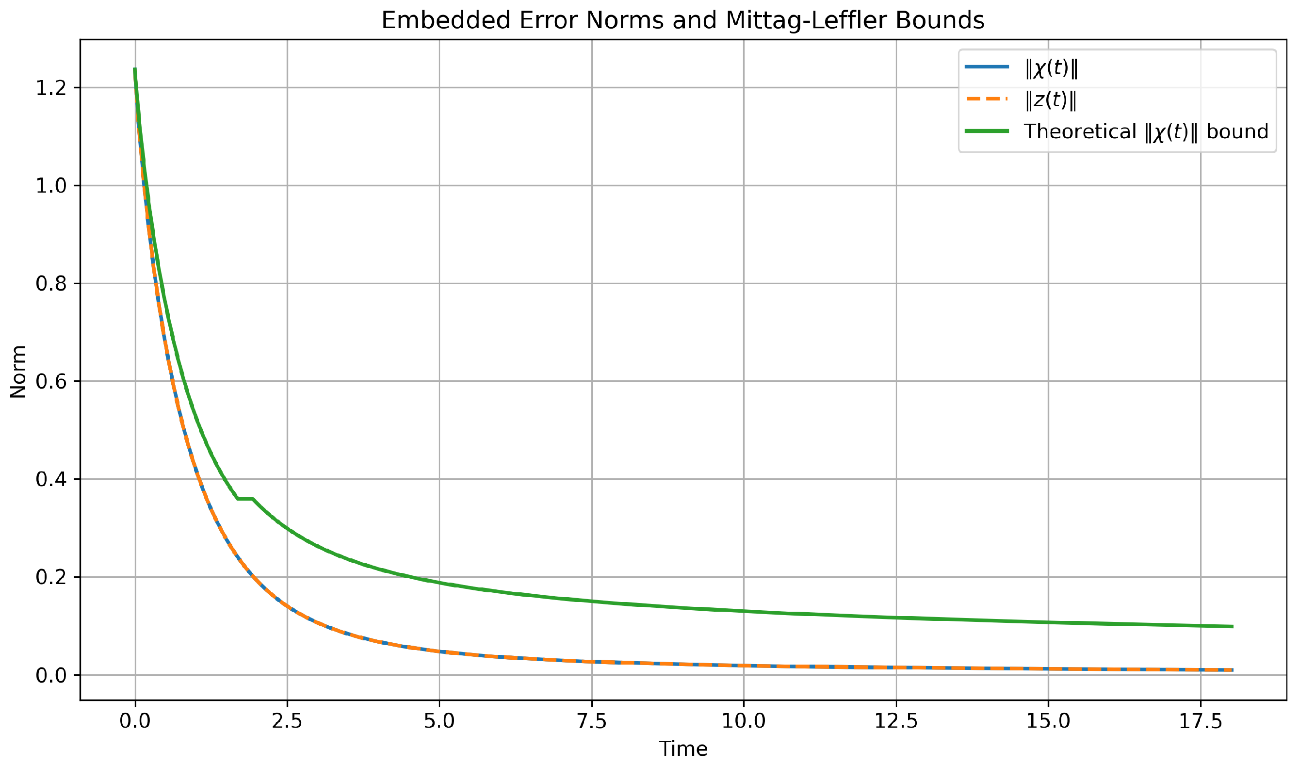
Figure 1 reports the trajectories of $\parallel \chi \left(t\right)\parallel$ and $\parallel z\left(t\right)\parallel$, together with the theoretical Mittag-Leffler envelope predicted by Theorem 1. Since $z=\chi$ in the present benchmark, the two measured norms coincide and decay from $1.2359207$ to $9.9026\times {10}^{-3}$ at the end of the simulation. The theoretical bound remains above the simulated trajectory throughout the time horizon, with the normalized ratio $\parallel \chi \left(t\right)\parallel /\mathrm{bound}$ equal to 1 at $t=0$ and strictly below 1 afterward. The maximum value of the ratio is exactly $1.0$, which is consistent with initialization from the exact initial condition. These results numerically confirm the Mittag-Leffler estimate (81) and (82).

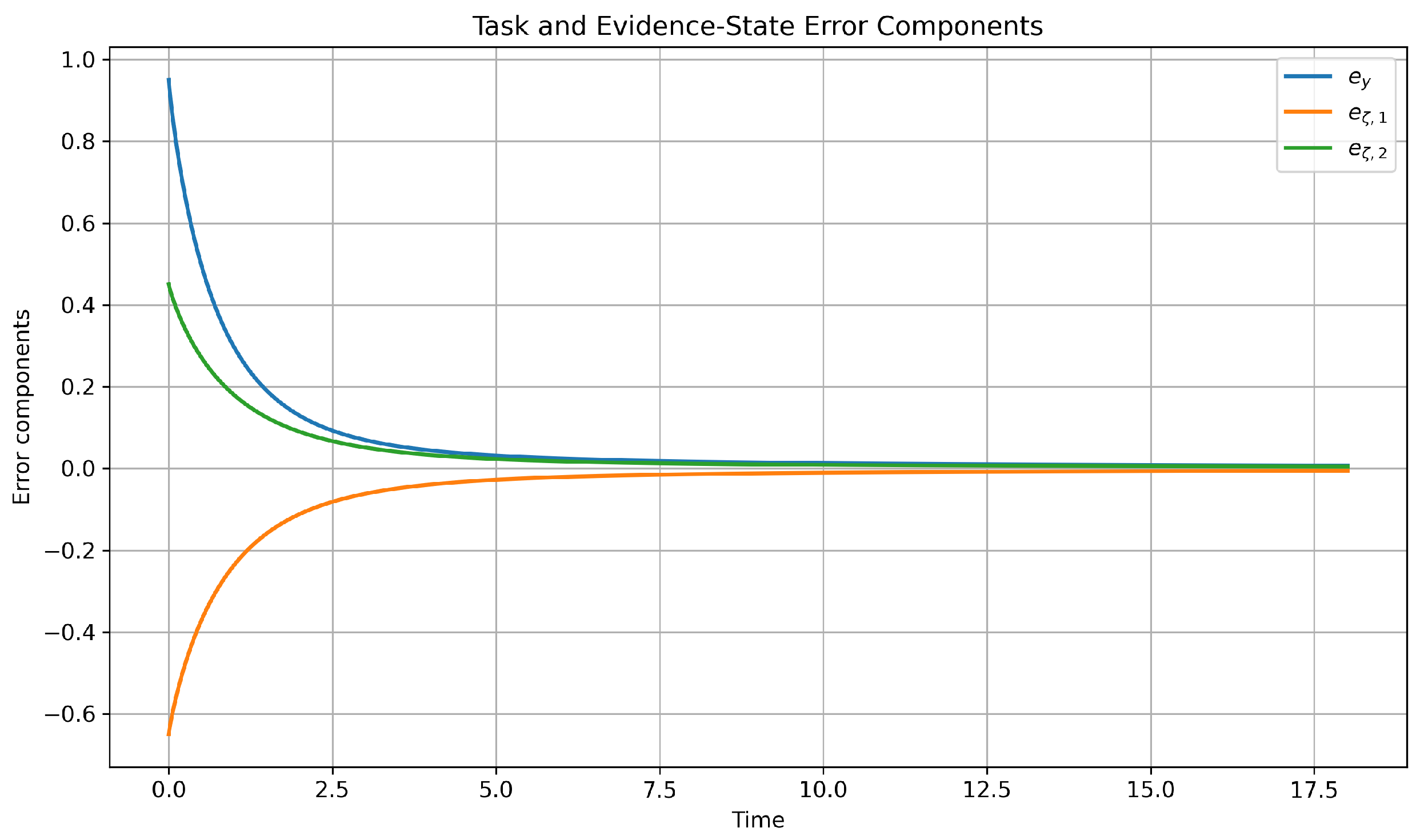
The decay of the individual error components is shown in Figure 2. The task tracking error $e_y\left(t\right)$ decreases from $0.95$ to zero, while the evidence-state errors $e_{\zeta ,1}\left(t\right)$ and $e_{\zeta ,2}\left(t\right)$ converge from $-0.65$ and $0.45$, respectively, toward zero. The convergence is smooth and monotone after the initial transient, which is consistent with the stable eigenstructure of the nominal closed loop and with the bounded residual term ${\Delta }_{\chi }$.

5.3. Intent-Evidence Convergence and Belief-State Behavior

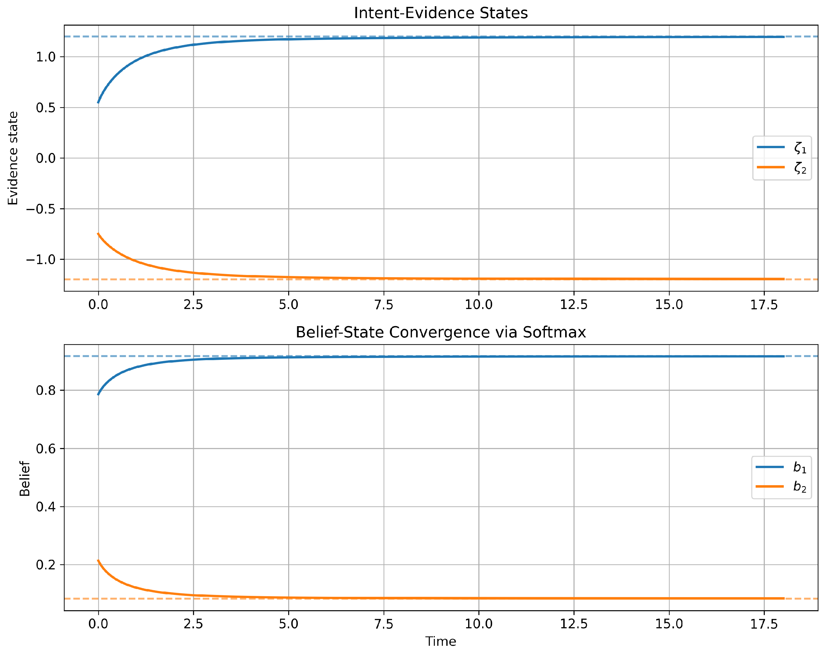
Figure 3 illustrates the convergence of the internal intent-evidence state and the corresponding softmax belief. The upper panel shows ${\zeta }_1\left(t\right)$ and ${\zeta }_2\left(t\right)$ converging toward the desired constant values ${\zeta }_{1,d}=1.2$ and ${\zeta }_{2,d}=-1.2$. The lower panel shows the associated belief components $b_1\left(t\right)$ and $b_2\left(t\right)$, obtained through the softmax map (59), converging close to the desired belief profile

$$b_d=\left[\begin{array}{c}0.9168273\\ 0.0831727\end{array}\right].$$

At the end of the simulation, the measured belief values are $b_1\left(18\right)\approx 0.916063$ and $b_2\left(18\right)\approx 0.083937$, which indicates accurate convergence of the accountability-related observer state. This result supports the practical relevance of the finite-dimensional intent-evidence realization introduced in Section 4.

5.4. Validation of the Conditional Safety Theorem

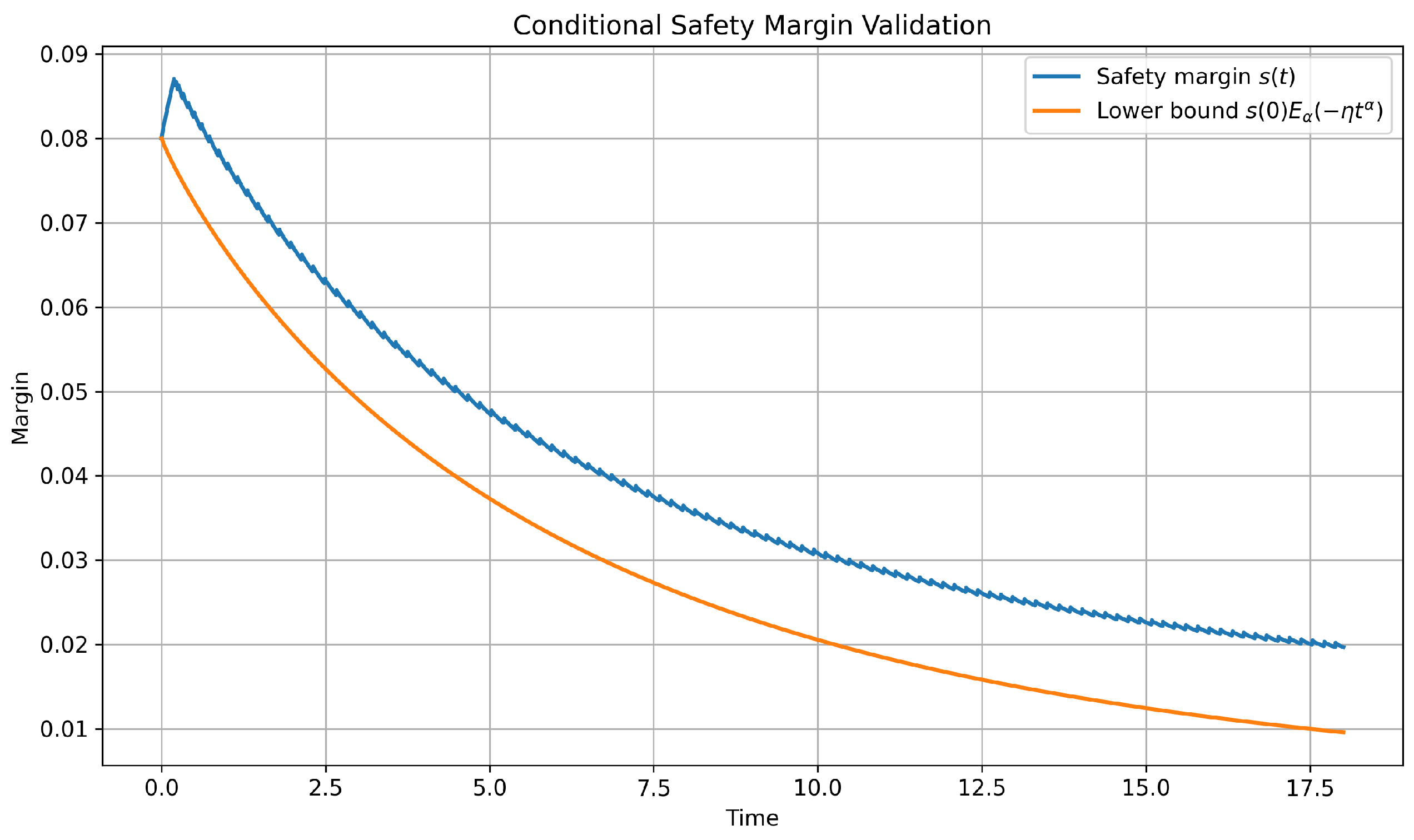
The conditional safety layer is validated in Figure 4, which shows the scalar safety margin $s\left(t\right)$ together with the lower bound $s\left(0\right)E_{\alpha }(-\eta t^{\alpha })$ predicted by Theorem 2. The safety margin remains strictly positive over the whole simulation interval, with minimum value $0.01968$. The trajectory stays above the comparison-theorem lower bound for all $t\in [0,T]$, which numerically confirms the forward-invariance conclusion of Theorem 2.

A notable aspect of Figure 4 is that the safety margin does not simply decay passively. Instead, the auxiliary safety correction causes an initial upward adjustment of the margin above its nominal reference profile, after which the margin gradually decreases while remaining positive. This illustrates that the scalar fractional safety channel can enforce the barrier condition without destroying the nominal regulation behavior.

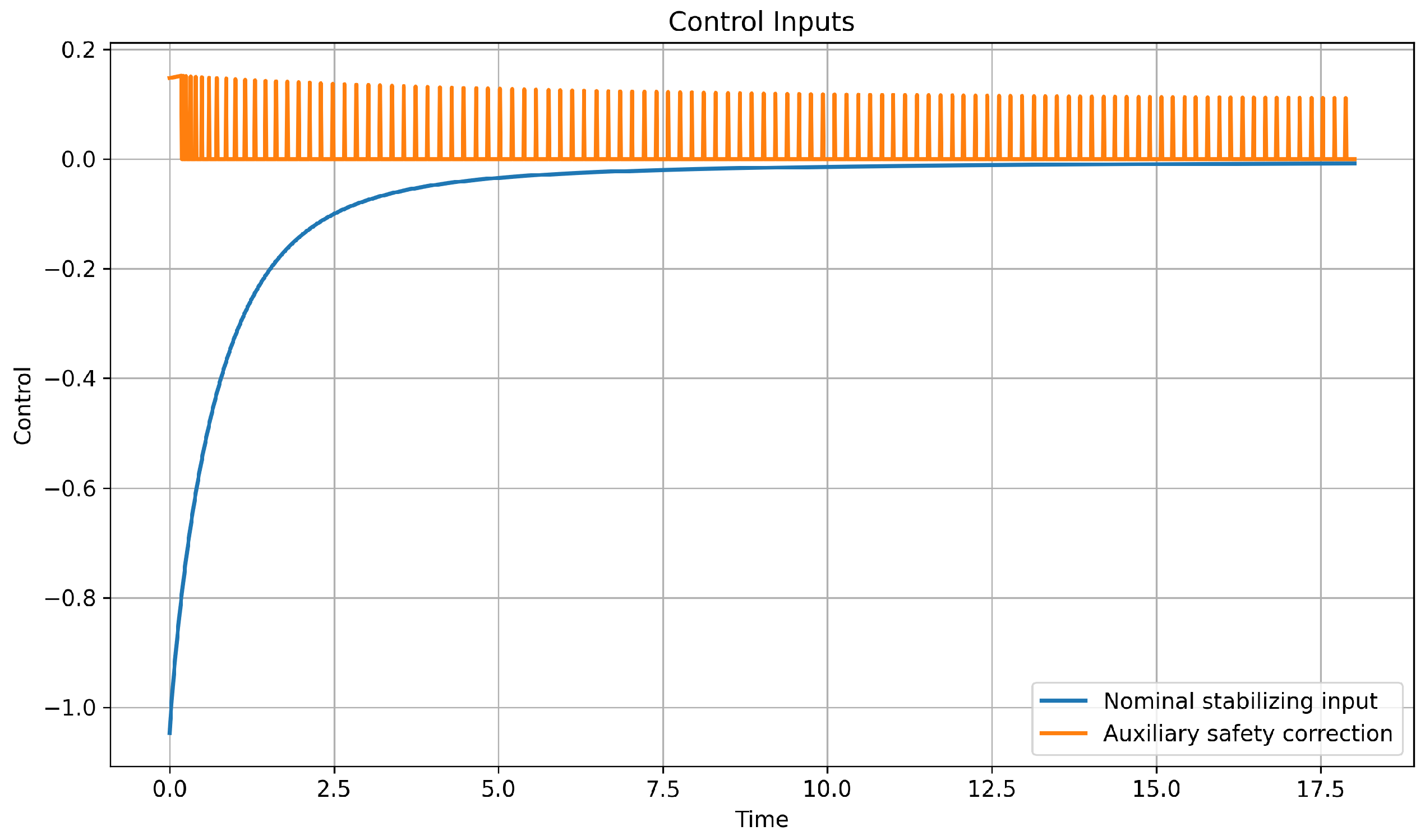
5.5. Control Effort and Non-Invasive Safety Correction

Figure 5 displays the two control channels. The nominal stabilizing input starts from approximately $-1.0475$ and decays toward zero, reflecting the progressive reduction of the regulation error. The auxiliary safety correction appears as a smaller positive pulse train that maintains the scalar safety margin. Quantitatively, the maximum absolute nominal control is $1.0475$, whereas the maximum safety correction is only $0.15215$. This indicates that the safety action remains smaller than the initial nominal transient stabilization effort and is therefore non-dominant in the present benchmark.

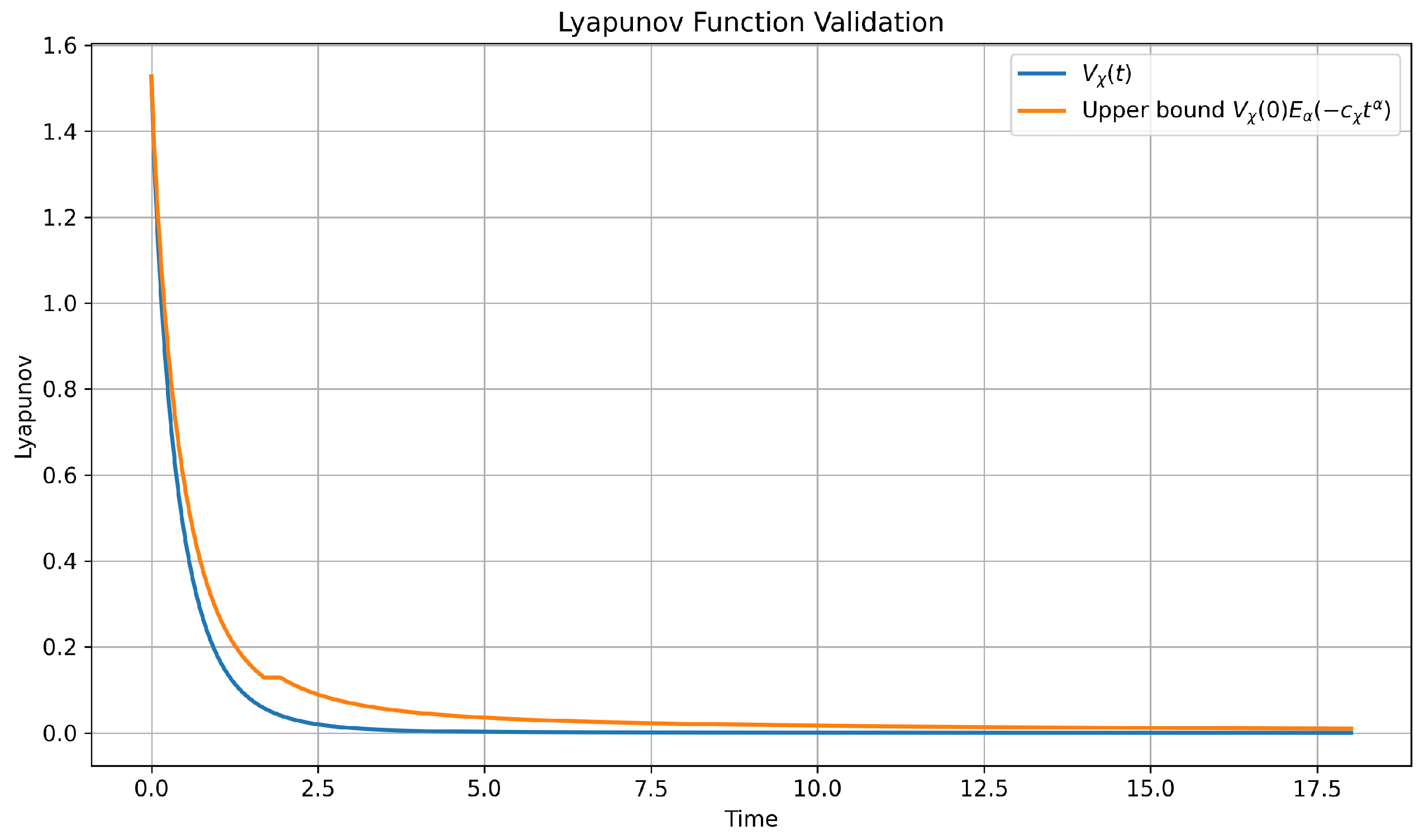
5.6. Lyapunov-Function Validation and Residual Analysis

Figure 6 compares the Lyapunov function $V_{\chi }\left(t\right)={\chi }^{\top }\left(t\right)P\chi \left(t\right)$ with the theoretical upper bound $V_{\chi }\left(0\right)E_{\alpha }(-c_{\chi }{t}^{\alpha })$ predicted by the proof of Theorem 1. The Lyapunov function decays monotonically, while the theoretical envelope remains above the simulated curve throughout the horizon. This provides direct numerical support for the comparison-based Lyapunov argument used in the proof.

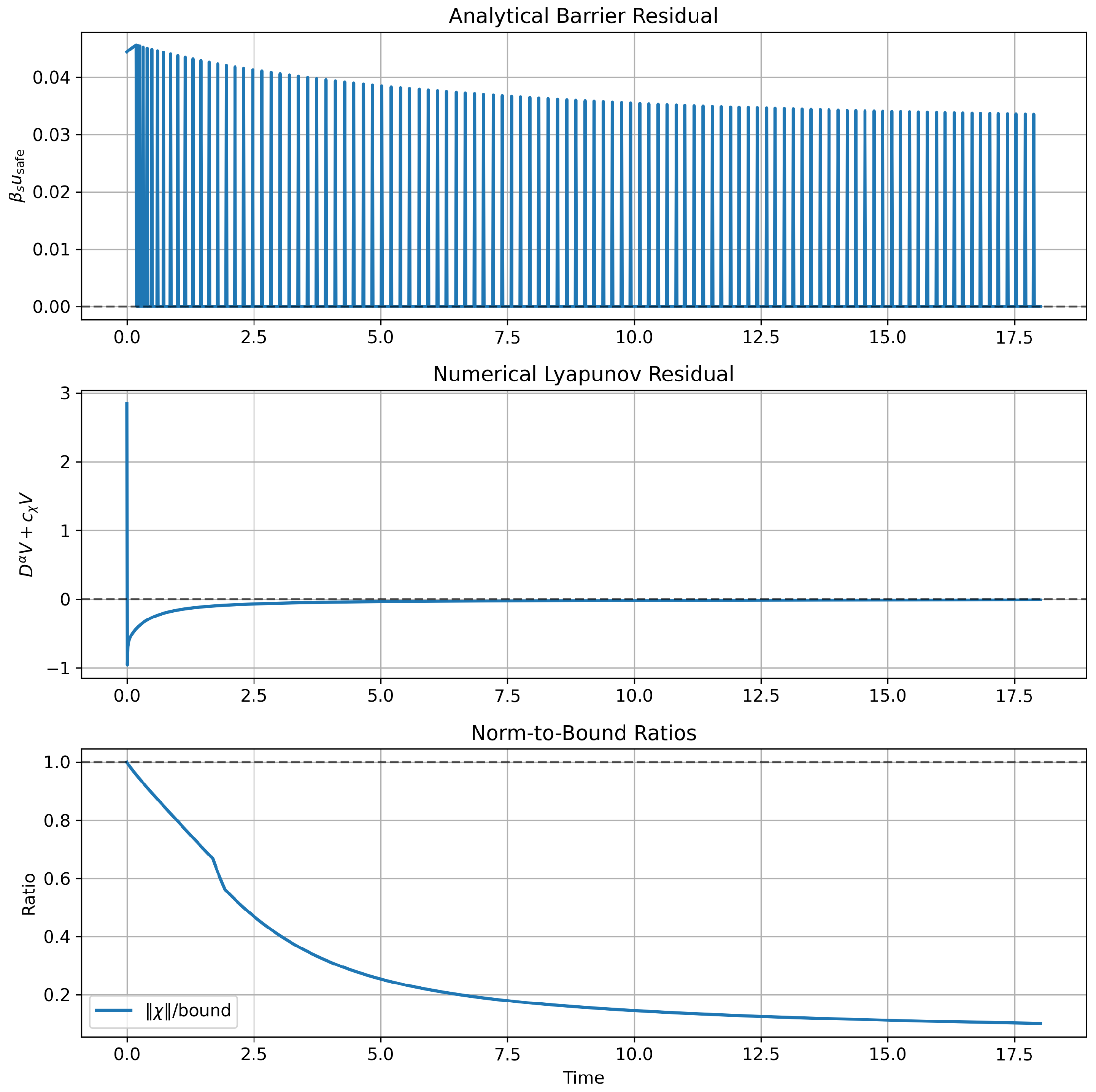
Figure 7 collects three additional theorem-validation diagnostics. The top panel reports the analytical barrier residual ${\beta }_s{u}_{\mathrm{safe}}$, which remains nonnegative by construction. The middle panel shows the numerical Lyapunov residual $D^{\alpha }V+c_{\chi }V$, computed from the L1 approximation of the Caputo derivative. A visible startup transient occurs at $t=0$, after which the residual becomes negative and gradually approaches zero from below. This initial spike is a numerical startup artifact of the Caputo derivative reconstruction rather than a failure of the analytical Lyapunov inequality. The bottom panel shows the ratio $\parallel \chi \left(t\right)\parallel /\mathrm{bound}$, which remains at or below 1 and decays monotonically after initialization.

Moreover, the Lyapunov-compatibility condition is satisfied exactly in this benchmark: the compatibility residual is identically zero because the safety correction is implemented through a decoupled auxiliary channel. This validates the special-case realization of Assumption 12.

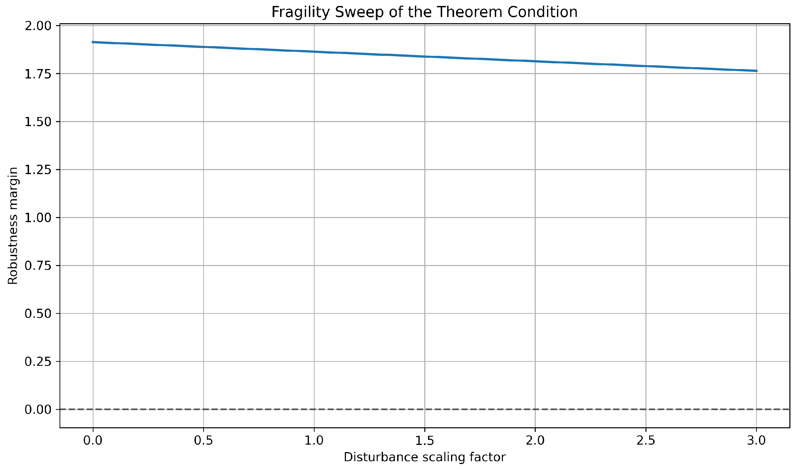
5.7. Robustness-Margin Sweep

To assess how conservative or fragile the nominal theorem condition is, Figure 8 reports the robustness margin

$${\lambda }_{\min }\left(Q\right)-2{\lambda }_{\max }\left(P\right)\overline{\delta }$$

as a function of a disturbance scaling factor. The margin decreases approximately linearly over the scanned range, but remains strictly positive throughout. This means that the closed-loop design is not operating close to the loss-of-validity threshold of Theorem 1; rather, it retains a comfortable stability margin under amplified disturbance levels.

5.8. Alpha Sweep and Integer-Order Baseline

To examine the influence of the fractional order and compare the proposed design with the matched integer-order case, we performed an $\alpha$-sweep over

$$\alpha \in \{1.00,0.95,0.90,0.80,0.70\}.$$

All cases use the same initial conditions, target response-time specification, and control structure. The case $\alpha =1.00$ is treated as the integer-order baseline.

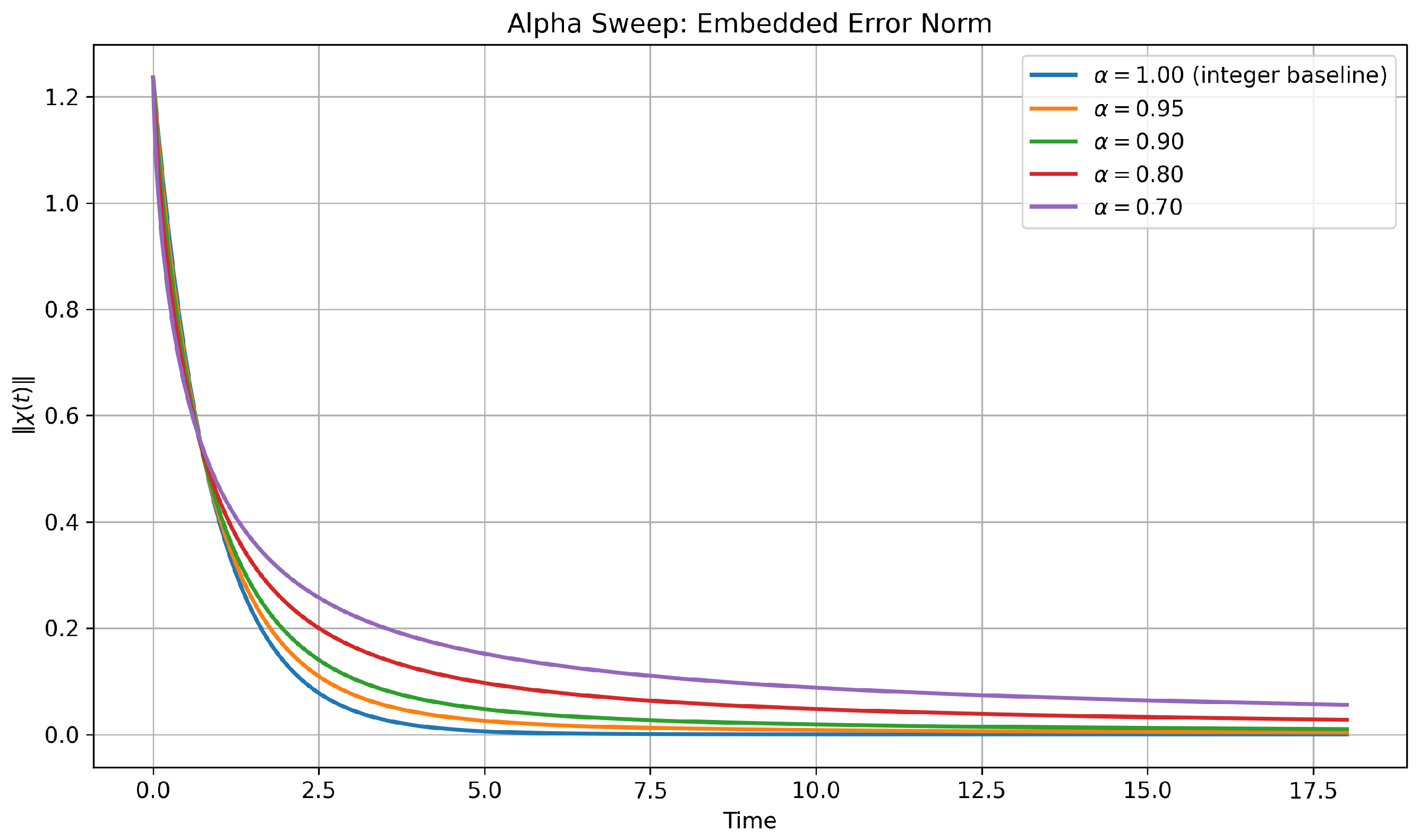
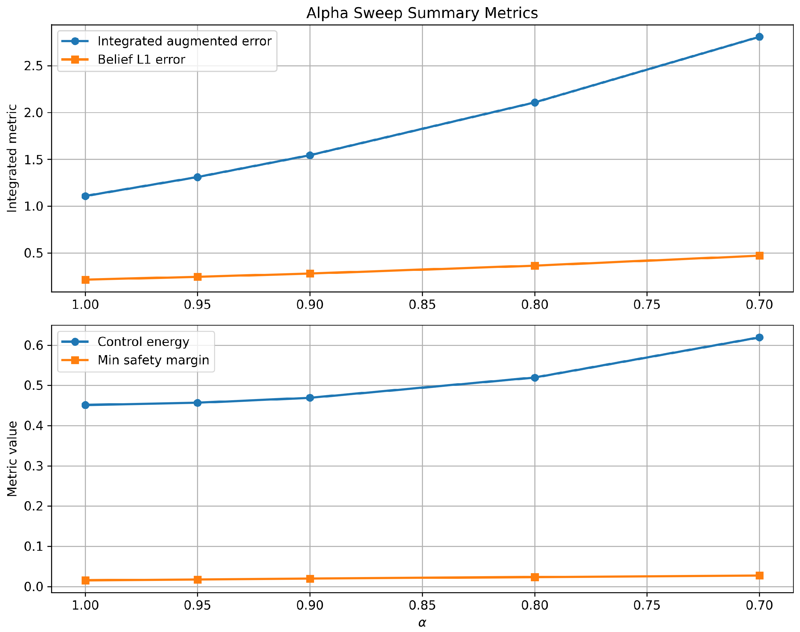
Figure 9 shows that the augmented error decays progressively more slowly as $\alpha$ decreases. This trend is quantified in Figure 10. The integrated augmented error increases from $1.1074$ for $\alpha =1.00$ to $1.3100$, $1.5438$, $2.1075$, and $2.8090$ for $\alpha =0.95,0.90,0.80,$ and $0.70$, respectively. Likewise, the integrated belief error increases from $0.2133$ at $\alpha =1.00$ to $0.2437$, $0.2786$, $0.3631$, and $0.4693$ as $\alpha$ decreases. The control energy also increases monotonically from $0.4512$ at $\alpha =1.00$ to $0.6190$ at $\alpha =0.70$.

At the same time, the minimum safety margin increases from $0.01548$ for the integer-order baseline to $0.01755$, $0.01968$, $0.02348$, and $0.02715$ as $\alpha$ decreases. The numerical evidence therefore suggests a safety–performance trade-off across the fractional-order family: larger $\alpha$ values yield faster regulation and smaller terminal error, whereas smaller $\alpha$ values produce more conservative trajectories with larger maintained proxemic margins.

These results do not claim empirical superiority of fractional order over the integer-order baseline. Rather, they demonstrate that varying $\alpha$ induces a systematic continuum of closed-loop behaviors and therefore that the fractional order acts as a meaningful design parameter within the present theorem-validation framework.

5.9. Step-Size Convergence Study

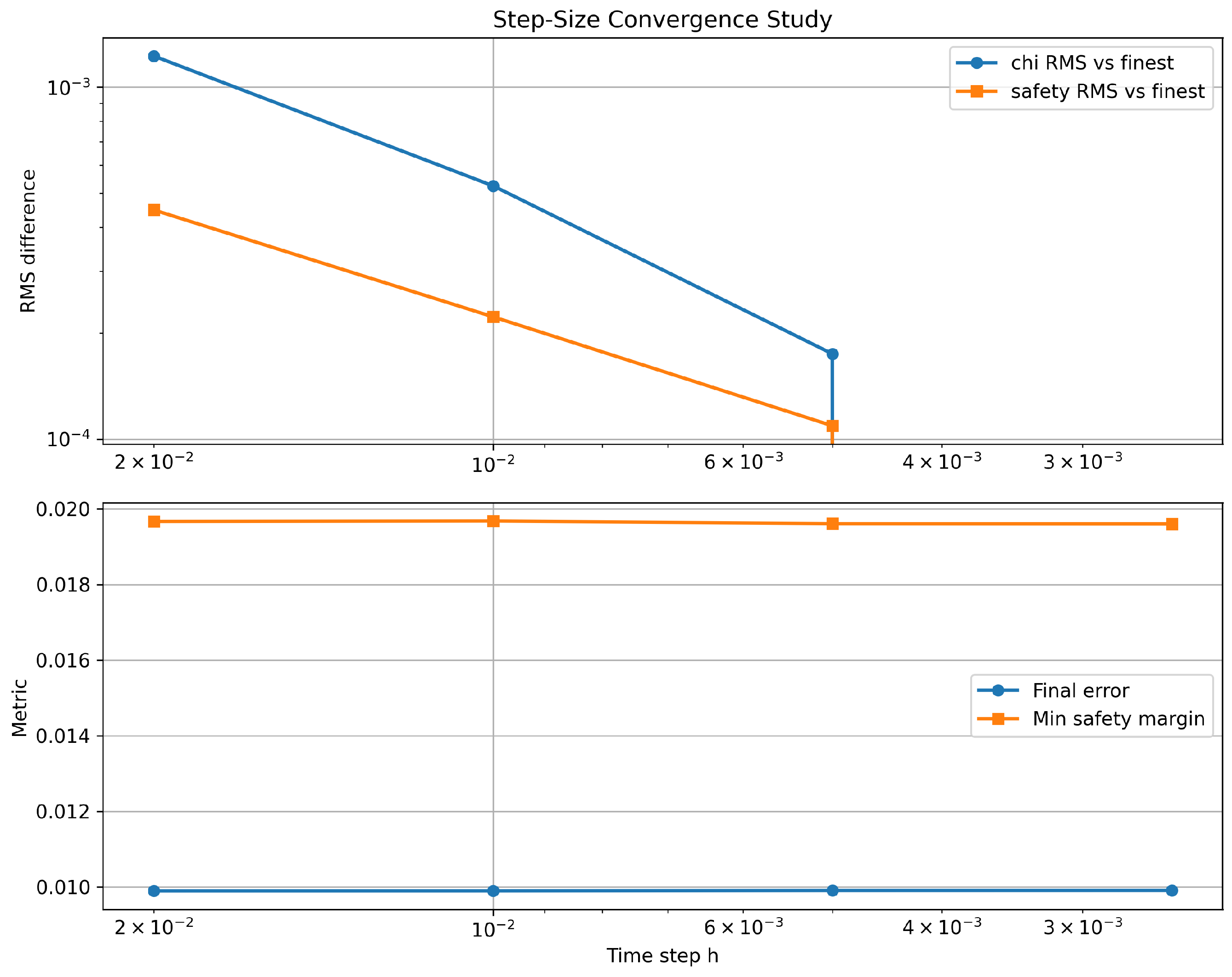
To examine whether the observed behaviors could be numerical artifacts of the Caputo discretization, a step-size convergence study was performed using

$$h\in \{0.02,0.01,0.005,0.0025\}.$$

The finest-grid simulation ($h=0.0025$) was used as the reference solution.

The RMS difference of the augmented error norm with respect to the finest grid decreases from $1.23\times {10}^{-3}$ at $h=0.02$ to $5.24\times {10}^{-4}$ at $h=0.01$ and to $1.75\times {10}^{-4}$ at $h=0.005$. The RMS difference of the safety margin similarly decreases from $4.48\times {10}^{-4}$ to $2.22\times {10}^{-4}$ and then to $1.09\times {10}^{-4}$ under the same refinement sequence. Meanwhile, the final augmented error norm remains nearly unchanged, varying only between $9.90\times {10}^{-3}$ and $9.91\times {10}^{-3}$, and the minimum safety margin remains stable around $1.96\times {10}^{-2}$.

These results indicate that the reported trajectories and performance metrics are numerically stable under grid refinement and are therefore not attributable to accumulated discretization errors.

Figure 11 presents the root mean square discrepancy between the augmented error norm and the safety margin relative to the finest-grid reference solution, along with the final error norm and the minimum safety margin evaluated over the range of tested step sizes.

5.10. Higher-Intent, Noisy-Observation, and Uncertainty Validation

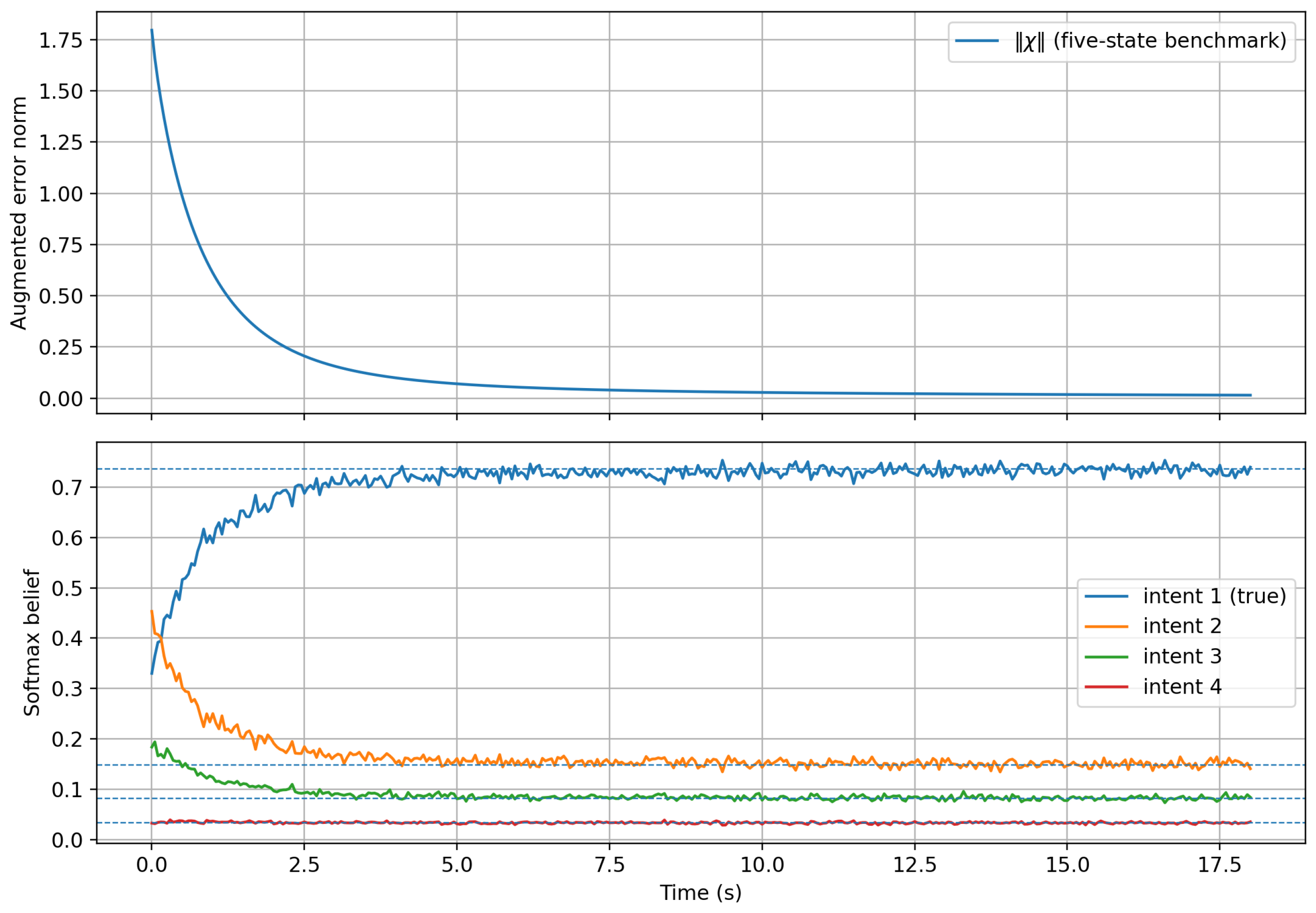
The previous simulations validate the theorem in a two-intent setting. To examine whether the intent-evidence realization remains meaningful for a richer accountability channel, we also simulated a four-intent case with

$${\zeta }_d={\left[\begin{array}{cccc}1.8& 0.2& -0.4& -1.3\end{array}\right]}^{\top },b_d=\mathrm{softmax}\left({\zeta }_d\right),$$

so that the desired true-intent belief is $b_{1,d}=0.7365$. The augmented state is enlarged to

$$\chi ={\left[\begin{array}{ccccc}{e}_y& e_{\zeta ,1}& e_{\zeta ,2}& e_{\zeta ,3}& e_{\zeta ,4}\end{array}\right]}^{\top }\in {\mathbb{R}}^5.$$

The belief reconstruction is evaluated from noisy measured evidence ${\zeta }_{\mathrm{meas}}=\zeta +\nu$, where $\nu$ is zero-mean bounded-variance observation noise. Figure 12 shows that the five-state augmented error still converges and that the softmax belief of the true intent approaches the desired value despite noise-induced fluctuations. In the representative noisy trial, the final augmented error norm is $1.4657\times {10}^{-2}$, the final true-intent belief is $0.7397$, and the RMS belief error is $8.34\times {10}^{-2}$.

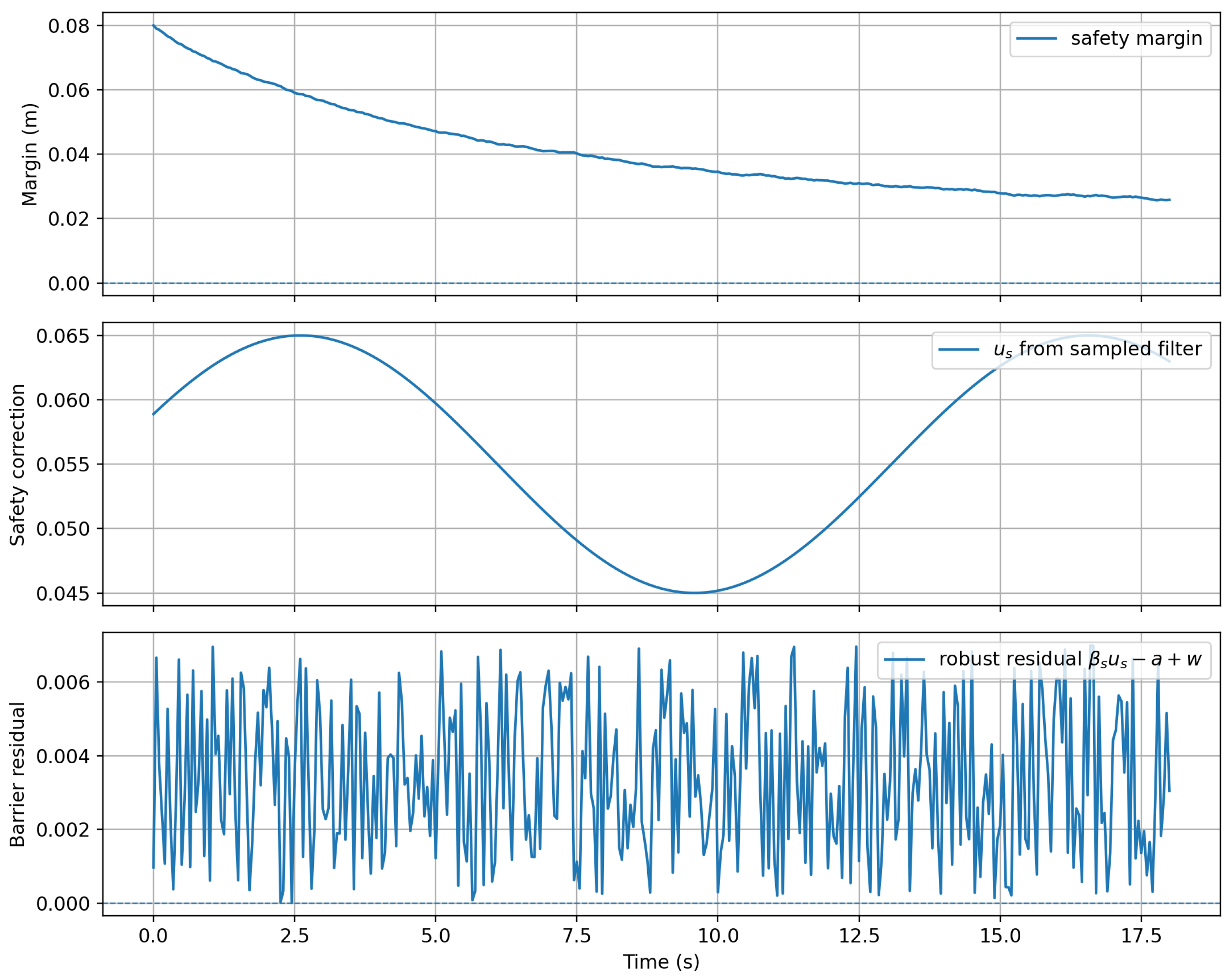
To reduce the idealization of the safety channel, the same scenario was also tested with a robust sampled safety filter of the form (101). The scalar margin channel includes an approach disturbance and bounded residual noise. The minimal-intervention correction is computed as the smallest nonnegative action that compensates the worst-case approach term within the prescribed uncertainty bound. Figure 13 reports the resulting safety margin, safety correction, and robust barrier residual. The minimum safety margin remains positive at $2.57\times {10}^{-2}$ m, the maximum safety correction is $6.5\times {10}^{-2}$, and the minimum robust residual is $8.77\times {10}^{-6}$, indicating that the sampled barrier inequality is maintained in the tested noisy realization.

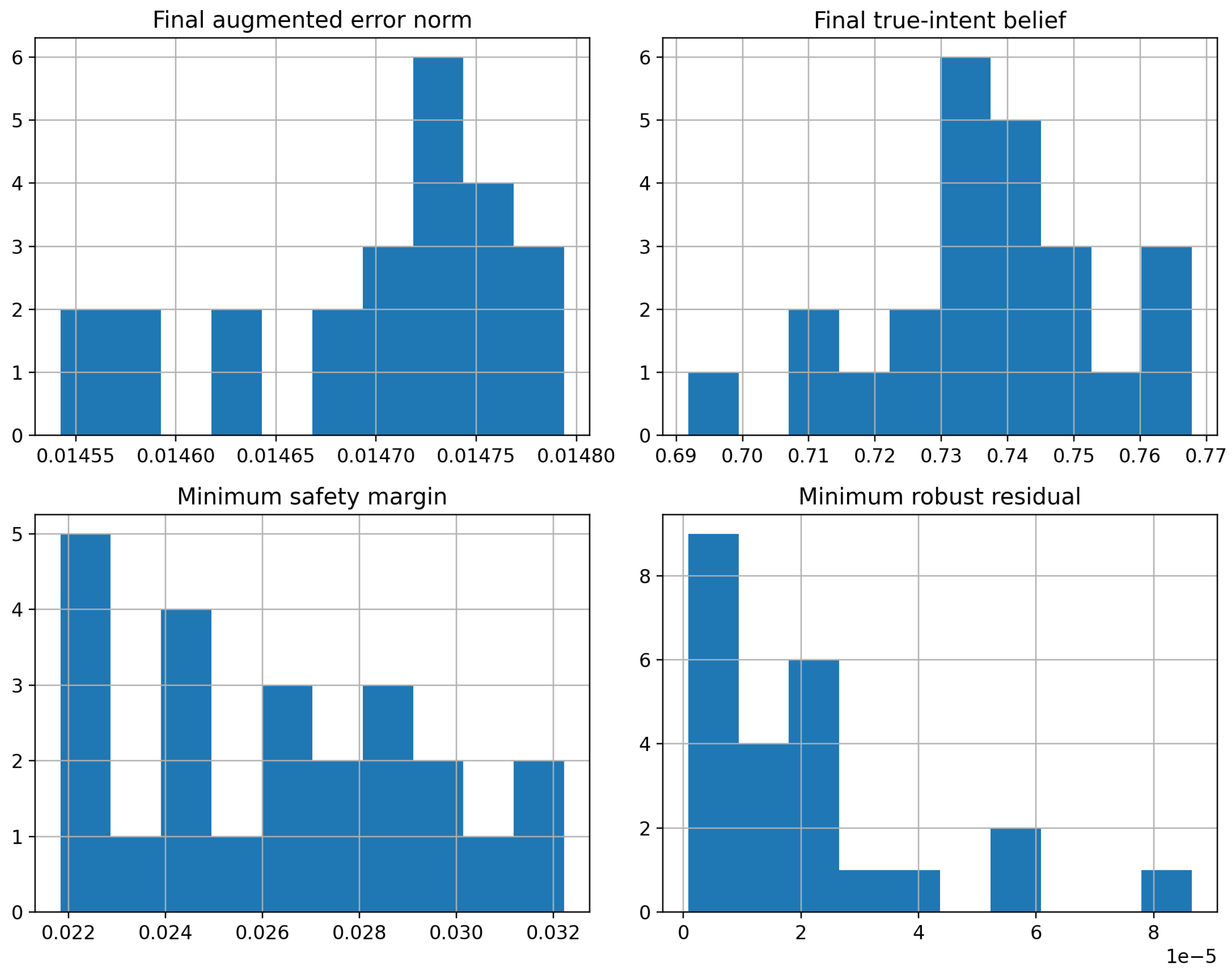
A small Monte Carlo stress test was then performed over 24 episodes, with observation-noise standard deviation varied between $0.025$ and $0.10$ and disturbance scaling varied between $0.75$ and $1.25$. Figure 14 summarizes the distributions of final augmented error, final true-intent belief, minimum safety margin, and minimum robust barrier residual. Across all episodes, the mean final augmented error norm is $1.4699\times {10}^{-2}$, the maximum final augmented error norm is $1.4794\times {10}^{-2}$, the mean final true-intent belief is $0.7375$, and the smallest final true-intent belief is $0.6918$. The minimum safety margin over all episodes is $2.18\times {10}^{-2}$ m and the smallest robust residual remains positive at $8.10\times {10}^{-7}$. These additional tests do not replace real-robot experiments, but they show that the theorem-validation behavior persists under higher intent cardinality, noisy belief reconstruction, and bounded safety-channel uncertainty.

5.11. Summary Metrics and Theory Validation

The main quantitative performance indicators of the base-case simulation are collected in

Table 2. Summary performance metrics of the base-case simulation.

Metric	Value
Initial $\parallel \chi \left(0\right)\parallel$	$1.2359207$
Final $\parallel \chi \left(T\right)\parallel$	$9.9026\times {10}^{-3}$
Integrated tracking error	$1.08896$
Integrated augmented error	$1.54382$
Integrated belief error	$0.27859$
Control energy	$0.46895$
Minimum safety margin	$0.01968$
Final safety margin	$0.01968$
Maximum $|u_{\mathrm{track}}|$	$1.0475$
Maximum $u_{\mathrm{safe}}$	$0.15215$
Settling time (2%)	$8.0$ s
Maximum $\parallel \chi \parallel /\mathrm{bound}$	$1.0$
Final belief $b_1\left(T\right)$	$0.916063$
Final belief $b_2\left(T\right)$	$0.083937$

. The final error norm is below ${10}^{-2}$, the minimum safety margin remains positive, the control energy remains moderate, and the maximum norm-to-bound ratio is exactly 1. Taken together, these results provide a consistent numerical validation of the main theoretical claims.

We may now summarize the theorem-validation outcome as follows:

(V1)

Validation of Theorem 1. The augmented error norm and Lyapunov function both decay in agreement with the predicted Mittag-Leffler envelopes, and the robustness condition ${\lambda }_{\min }\left(Q\right)-2{\lambda }_{\max }\left(P\right)\overline{\delta }>0$ is satisfied with margin $1.8641$. The ratio $\parallel \chi \parallel /\mathrm{bound}$ remains at or below 1 over the whole simulation.

(V2)

Validation of Theorem 2. The safety margin remains strictly positive and above the comparison-theorem lower bound $s\left(0\right)E_{\alpha }(-\eta t^{\alpha })$, confirming forward invariance of the scalar safe set associated with the synthetic safety channel.

(V3)

Validation of Theorem 3. Since both the nominal stability condition and the safety condition are satisfied simultaneously, and since the compatibility residual is exactly zero, the simulation validates the combined accountability-aware stabilization with conditional safety preservation stated in Theorem 3.

(V4)

Validation against numerical-artifact concerns. The step-size convergence study confirms that the reported trajectories and summary metrics are stable under grid refinement, while the $\alpha$-sweep confirms that varying the fractional order produces a systematic family of safety–performance trade-offs rather than isolated numerical patterns.

(V5)

Validation under richer intent and noise conditions. The four-intent benchmark and Monte Carlo uncertainty tests show that the softmax evidence mechanism and safety-filter diagnostics remain coherent under noisy observations and bounded disturbance scaling.

Remark 23.

The present simulation is intentionally designed as a theorem-validation benchmark. In particular, the safety variable is implemented as a scalar fractional margin channel rather than as a full geometric robot–human distance barrier. This is fully consistent with the conditional safety framework of Section 4: the simulation validates the logical sufficiency of the barrier inequality and Lyapunov compatibility assumptions, while leaving application-specific synthesis of $u_s$ for concrete geometric robot models to future work.

5.11.1. Scope of the Validation

The simulations provide comparative numerical validation of the proposed theorem-oriented framework, including a matched integer-order baseline and an $\alpha$-sweep, but they do not constitute empirical real-robot validation. Experimental validation on robotic platforms and application-specific geometric safety synthesis remain directions for future work.

5.11.2. Real-World Implementation Pathway

A practical robotic implementation would instantiate the abstract variables as follows: $x_r$ would be obtained from the robot localization and velocity-estimation stack, $x_h$ from human tracking or prediction, $s\left(t\right)$ from the measured robot–human distance or an anisotropic proxemic model, $\zeta \left(t\right)$ from the intent-evidence filter, and $u_s\left(t\right)$ from a sampled safety filter such as (101). Human–robot interaction data can therefore be used in two ways: first, to identify or bound the local embedding residual $\overline{\delta }$ and tune K, $\alpha$, and the accountability weights; second, to evaluate the episode-level accountability score (33) from logged proxemic, belief, smoothness, and rule-compliance variables. The current manuscript does not claim that these experiments have already been carried out; instead, it provides the mathematical and numerical structure needed to design such real-world tests.

The main difficulty in real data is that fractional-order memory couples the present control update to a history of noisy measurements. In simulation this requires careful initialization, bounded-noise modeling, and grid-refinement checks; on a robot, it also requires filtering, delay compensation, and explicit actuator/sensing constraints. These issues explain why the numerical results are presented as theorem-validation and stress-test evidence, while platform-level HRI experiments are left as the next validation stage.

6. Conclusions

This paper developed an accountability-aware fractional control framework for embodied intelligent systems in shared human environments. By combining a Caputo fractional-order stabilizing law, a finite-dimensional intent-evidence realization with softmax belief reconstruction, and a conditional proxemic safety layer, the proposed formulation unifies task regulation, interpretable interaction behavior, and safety preservation within a single control-oriented framework. Using fractional Lyapunov arguments and comparison-based analysis, sufficient conditions were established for the local Mittag-Leffler stability of the augmented error dynamics, while the forward invariance of the proxemic safe set was guaranteed through a fractional barrier inequality.

The numerical study provided several complementary forms of theorem-oriented validation. First, the base-case simulation confirmed the nominal stability and conditional safety results with a robustness margin of $1.8641$, a final augmented error norm below ${10}^{-2}$, and a strictly positive maintained safety margin. Second, the simulation parameters were re-expressed through a parameter-provenance layer linking theorem-level constants to interpretable quantities such as initial robot–human separation, minimum comfort distance, and target response times for tracking, evidence convergence, and safety recovery. Third, an $\alpha$-sweep with a matched integer-order baseline showed that the fractional order acts as a meaningful design parameter: as $\alpha$ decreases, the closed-loop response becomes progressively more conservative, yielding larger maintained safety margins at the cost of slower convergence, larger integrated error, and higher control effort. Finally, a step-size convergence study demonstrated that the reported trajectories and summary metrics remain stable under grid refinement, supporting that the observed patterns are not caused by accumulated numerical errors.

These results strengthen the original theorem-validation benchmark in two ways. On the one hand, they provide clearer system-level interpretation of the numerical constants and therefore improve the transparency of the simulation design. On the other hand, they show that the fractional order induces a systematic family of safety–performance trade-offs rather than merely isolated numerical patterns. At the same time, the numerical evidence does not establish empirical superiority of fractional order over the integer-order baseline in the present synthetic benchmark; rather, it shows that the fractional order provides a tunable continuum of behaviors within the proposed framework.

The study differs from many existing social-navigation or HRI models by embedding intent confidence, proxemic compliance, smoothness, rule consistency, and communication–execution consistency directly into a control-oriented accountability output, rather than treating them only as post hoc evaluation metrics. It also differs from standard fractional-control studies by coupling Mittag-Leffler regulation with observer-dependent intent evidence and a proxemic safety layer. Thus, the main contribution is not a new social-navigation planner alone, nor a fractional stabilizer alone, but an integrated framework in which accountability-related quantities enter the closed-loop stability and safety analysis.

The present study remains intentionally theorem-oriented. The added sampled filter and noisy multi-intent tests make the validation less idealized, but the results still do not constitute empirical real-robot validation. In particular, the continuous-time safety theorem is conditional on the existence of an auxiliary correction satisfying the fractional barrier and Lyapunov-compatibility inequalities, while the proposed sampled quadratic program provides a practical verification/synthesis route for a specified platform. Future work will therefore focus on full geometric robot–human barrier synthesis, identification of the fractional embedding from real HRI logs, optimization of controller and accountability weights from experimental data, and deployment on embodied robotic platforms with human participants.