A Symmetry-Based Strapdown Attitude Update Algorithm Suitable for Low-Dynamic Motion

Abstract

The attitude update algorithm is the core component determining the navigation accuracy of strapdown INS, directly affecting velocity and position solution precision. Existing algorithms were designed typically based on first-order Taylor expansions of the rotation vector differential equation, inevitably introducing approximation errors. To obtain precise attitude information under low-dynamic motion, a symmetry-based strapdown attitude update algorithm is proposed. An auxiliary frame is constructed in which the angular-rate vector becomes constant. This transformation exploits the rotational symmetry inherent in rigid-body rotation. The attitude update reduces to a steady rotation about a fixed axis. Consequently, the attitude update in this frame can be performed without approximation errors. The performance of the proposed algorithm under low-dynamic motion was sufficiently compared with that of the traditional algorithms in the simulation. The simulation results demonstrate that the proposed method outperforms traditional ones with an accuracy improvement of five orders of magnitude, validating its suitability for low-dynamic motion.

1. Introduction

In a strapdown inertial navigation system (INS), inertial sensors, i.e., gyros and accelerometers, are directly mounted to the vehicle body frame [1,2,3]. This physical connection configuration makes the gyro and accelerometer highly susceptible to carrier vibrations and environmental disturbances, particularly in dynamic or vibration environments, which can significantly degrade the accuracy of the strapdown INS. Since the strapdown INS replaces a physical platform with a mathematical one, its core algorithms must perform real-time computation to resolve the carrier’s attitude. Therefore, the calculation of vehicle attitude is the core part of a strapdown INS [4,5].

The study of attitude update algorithms based on the rotation vector differential equation traces its origins to Bortz’s seminal work in 1971 [6]. Savage advanced an attitude update framework by employing equivalent rotation vectors to significantly improve attitude update accuracy [7]. Using Taylor series expansion in powers of time, Wang presented a new coning correction algorithm, which can recover the maneuver accuracies of known coning algorithms [8]. Based on the functional iterative integration and Chebyshev polynomials, Wu proposed a novel inertial navigation attitude algorithm that reduces the coning error that has perplexed the navigation community for long [9]. Yang proposed a novel attitude algorithm based on a pseudo-linear model in the geographic frame, and has higher algorithm accuracy under the condition of high dynamics and large maneuver [10]. Furthermore, Yang proposed a new attitude update algorithm by approximating the angular velocity function using Legendre polynomials, with the numerical method of the differential equation at its core [11]. Yan proposed a new numerical attitude updating algorithm deduced on the basis of Taylor series expansion according to the differential equation of the attitude matrix with implicit non-commutativity error compensation [12]. Wang described a strapdown INS attitude numerical updating algorithm based on Adams-PECE, and this algorithm does not need to calculate rotation errors [13]. Lu proposed a high-dynamic attitude updating algorithm based on sine function fitting of angular velocity and the sixth-order Taylor series expansion of the equivalent rotation vector [14]. Liang proposed an angular-rate attitude algorithm based on multi-interval information correction to increase the attitude update frequency and calculation accuracy [15]. Naidu proposed novel attitude estimation with Singular Value Decomposition (SVD) for stable, computationally efficient estimation [16]. Patera proposed attitude propagation for a slewing angular-rate vector [17]. It is applicable only to specific types of motion, such as those where the angular velocity is a known function or those exhibiting coning motion. All existing algorithms are primarily designed for error compensation in high-dynamic or high-rotation-rate environments. They implicitly rely on assumptions such as time-scale separation, small-angle approximation, and the dominance of non-commutative errors. However, these assumptions all become invalid under low-dynamic motion.

Aiming at the mentioned problems, a symmetry-based strapdown attitude update algorithm suitable for low-dynamic motion is proposed in this paper. The proposed algorithm integrates an auxiliary frame in which the angular-rate vector becomes constant in the existing attitude update framework. The attitude update reduces to a steady rotation about a fixed axis. Consequently, the attitude update in this frame can be performed without approximation errors. This transformation exploits the rotational symmetry inherent in rigid-body rotation [18,19,20]. Furthermore, it systematically evaluates the applicability of the algorithm under this motion. The subsequent sections address the following: Section 2 presents the traditional methods. In Section 3, a proposed method is described. Section 4 describes the error analysis of proposed algorithm under low-dynamic motion. Section 5 details the simulation results and discussion. The conclusion is provided in Section 6.

2. Traditional Attitude Update Algorithm

Within the attitude update cycle H, the angular velocity of the vehicle is assumed to be representable by a second-order polynomial in time:

$$\omega \left(t+\tau \right)=a+2b\tau +3c{\tau }^2$$

(1)

where $a$, $b$, and $c$ are coefficients. The gyroscope samples the angular velocity twice during each update cycle, i.e., H = 2h. Three angular velocity measurements can be obtained over the time interval [t, t + H], including the sample from the previous update cycle’s termination time.

The polynomial coefficients can then be expressed in terms of these sampled angular velocity measurements as follows:

$$\begin{array}{l}a={\omega }_0\\ b=\left(4{\omega }_1-3{\omega }_0-{\omega }_2\right)/2H\\ c=2\left({\omega }_2-2{\omega }_1+{\omega }_0\right)/3H^2\end{array}$$

(2)

The integral of (1) over interval H yields the following angular increment:

$$\alpha =aH+b{H}^2+c{H}^3$$

(3)

In algorithm design, the differential equation of the rotation vector is typically approximated as

$$\dot{\varphi }\approx {\omega }_{ib}^b+{\displaystyle \frac{1}{2}}\alpha \times {\omega }_{ib}^b$$

(4)

where $\alpha ={\displaystyle \int {\omega }_{ib}^{b}dt}$ represents the angular increment of the carrier.

Integrating (4) over the attitude update cycle H gives the following:

$$\Delta \varphi =\alpha +{\displaystyle \frac{1}{2}}{\displaystyle {\int }_t^{t+H}\alpha \times {\omega }_{ib}^{b}dt}$$

(5)

Using Taylor series expansion combined with (2), the computational value for the rotation vector increment is derived as

$$\begin{array}{l}\Delta \widehat{\varphi }=\alpha +h^2{\displaystyle \sum _{i=0}^1{\displaystyle \sum _{j=i+1}^2{K}_{ij}({\omega }_i\times {\omega }_j)}}\\ \alpha ={\displaystyle \frac{H}{6}}({\omega }_0+4{\omega }_1+{\omega }_2)\end{array}$$

(6)

where $K_{ij}$ is an undetermined coefficient for the cross-product terms of angular rates, and $\alpha$ denotes the angular increment value during the velocity update cycle H.

When the body performs a typical coning motion, the angular velocity of the body frame relative to the inertial frame is [17]

$${\omega }_{ib}^b(t)=\left[\begin{array}{c}-2\Omega {\sin }^2({\displaystyle \frac{\varphi }{2}})\\ -\Omega \sin \varphi \sin \Omega t\\ \Omega \sin \varphi \cos \Omega t\end{array}\right]$$

(7)

where $\varphi$ is the coning half-apex angle and $\Omega$ denotes the coning frequency.

Substituting the angular velocity of the carrier in a typical coning motion into (5) yields the true value of the rotation vector increment over interval H.

$$\Delta \varphi =\left[\begin{array}{l}\Delta {\varphi }_x\\ \Delta {\varphi }_y\\ \Delta {\varphi }_z\end{array}\right]=\left[\begin{array}{l}-2{\sin }^2(\varphi /2)\sin (\Omega H)\\ -2\sin \varphi \sin (\Omega H/2)\sin \Omega [(t+H/2)]\\ 2\sin \varphi \sin (\Omega H/2)\cos \Omega [(t+H/2)]\end{array}\right]$$

(8)

The algorithmic design principle requires equality between the true and computed rotation vector increments, i.e.,

$$\Delta \widehat{\varphi }=\Delta \varphi$$

(9)

Substituting (6) and (8) into (9) yields the two-interval coning compensation algorithm for angular velocity [21]:

$$\stackrel{⌢}{\beta }=\alpha +h^2\left({\displaystyle \frac{1}{45}}{\omega }_0\times {\omega }_2+{\displaystyle \frac{28}{45}}{\omega }_1\times {\omega }_2\right)$$

(10)

where $\alpha ={\displaystyle \frac{H}{6}}({\omega }_0+4{\omega }_1+{\omega }_2)$, $H=2h$.

The derived attitude update algorithm, as presented in (4), is based on the equivalent rotation vector approximation. This approximation inherently introduces integration errors during attitude computation, as it neglects the higher-order terms in the Taylor series expansion of the rotation vector’s differential equation.

3. Proposed Attitude Update Algorithm

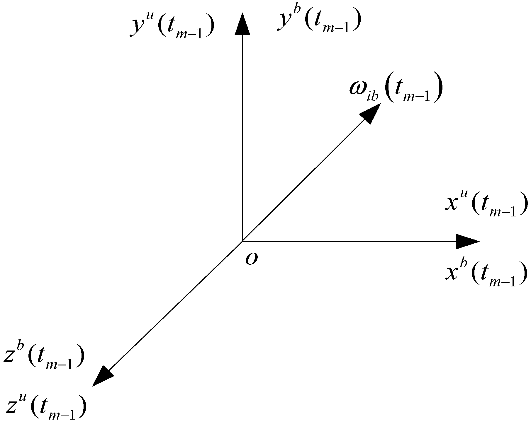
To eliminate the approximation errors existing in traditional algorithms and simplify the numerical integration of angular velocity ${\omega }_{ib}\left(t\right)$, an auxiliary frame, $u$ frame, is introduced in the existing attitude update framework. The reason for its introduction is that integrating a constant vector is significantly easier and more accurate than integrating a varying one. 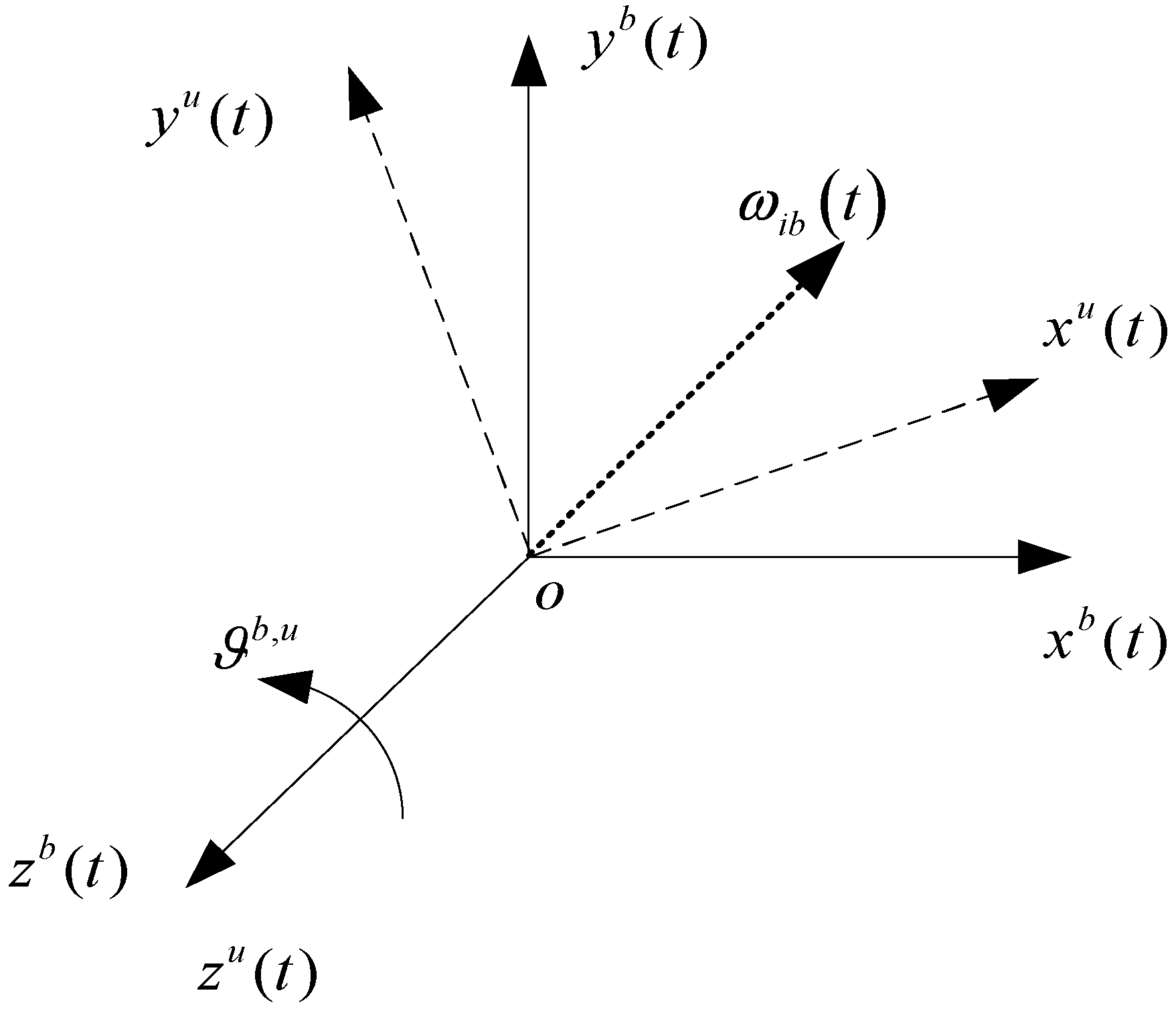At the start of each attitude update cycle $t_{m-1}$, the $b$ frame and $u$ frame coincide, and their spatial relationship at $t_{m-1}$ is shown in Figure 1. In each attitude update cycle at any time, the $u$ frame rotates at a constant angular velocity around the z-axis of the $b$ frame. The spatial relationships among the $b$ frame, $u$ frame, and angular velocity vector ${\omega }_{ib}\left(t\right)$ at any time $t\in \left[t_{m-1},t_m\right]$ are illustrated in Figure 2.

As shown in Figure 1, the $b$ frame and $u$ frame coincide at the start of each attitude update cycle $t_{m-1}$. So, one has

$${\omega }_{ib}^u(t_{m-1})={\omega }_{ib}^b(t_{m-1})$$

(11)

Figure 2 illustrates that at any time $t\in \left[t_{m-1},t_m\right]$, the $u$ frame rotates at a constant angular velocity ${\vartheta }^{b,u}$ around the z-axis of the $b$ frame. This implies a fixed spatial relationship between the $u$ frame and the angular velocity vector ${\omega }_{ib}\left(t\right)$ at $t\in \left[t_{m-1},t_m\right]$. Consequently, the projection of ${\omega }_{ib}\left(t\right)$ onto the $u$ frame remains constant, satisfying the following relation:

$${\omega }_{ib}^u(t)={\omega }_{ib}^u(t_{m-1})$$

(12)

Using (11) and (12), one obtains

$${\omega }_{ib}^u(t)={\omega }_{ib}^b(t_{m-1})$$

(13)

Given the definition of the $u$ frame, ${\vartheta }^{b,u}$ denotes the angular velocity of the $u$ frame relative to the $b$ frame. So, the absolute angular velocity vector ${\omega }_{iu}^u\left(t\right)$ can be expressed as the sum of the gyroscope output projected onto the $u$ frame and the rotational angular velocity ${\vartheta }^{b,u}$.

$${\omega }_{iu}^u(t)={\omega }_{ib}^u(t)+{\vartheta }^{b,u}$$

(14)

Substituting (12) into (14) yields

$${\omega }_{iu}^u(t)={\omega }_{ib}^b(t_{m-1})+{\vartheta }^{b,u}$$

(15)

where ${\omega }_{ib}^b\left(t_{m-1}\right)$ represents the gyroscope output at $t_{m-1}$ and ${\vartheta }^{b,u}$ is the rotational angular velocity of the $u$ frame relative to the $b$ frame, that is, the rotational angular velocity. Since both ${\omega }_{ib}^b\left(t_{m-1}\right)$ and ${\vartheta }^{b,u}$ are constant vectors, ${\omega }_{iu}^u\left(t\right)$ is also a constant vector.

The relationship between the rotation vector and the angular velocity vector ${\omega }_{iu}^u\left(t\right)$ is expressed by the following [14]:

$${\dot{\varphi }}^{iu}(t)={\omega }_{iu}^u\left(t\right)+{\displaystyle \frac{1}{2}}{\varphi }^{iu}\left(t\right)\times {\omega }_{iu}^u\left(t\right)+{\displaystyle \frac{1}{{\varphi }^{iu}{\left(t\right)}^2}}\left(1-{\displaystyle \frac{{\varphi }^{iu}\left(t\right)}{2}}\cot {\displaystyle \frac{{\varphi }^{iu}\left(t\right)}{2}}\right){\left({\varphi }^{iu}\left(t\right)\times \right)}^2{\omega }_{iu}^u\left(t\right)$$

(16)

As indicated by (15), ${\omega }_{iu}^u\left(t\right)$ is a constant vector, and its unit vector aligns with the rotation vector. Applying the vector cross-product identity, the latter two terms in (16) vanish. Thus, (16) can be rewritten as [2]

$${\dot{\varphi }}^{iu}(t)={\omega }_{iu}^u\left(t\right)$$

(17)

Subsequently, the vector ${\varphi }^{iu}(t)$ can be computed:

$${\varphi }^{iu}(t)={\displaystyle {\int }_{t_{m-1}}^t\left({\omega }_{ib}^b\left(t_{m-1}\right)+{\vartheta }^{b,u}\right)}\mathrm{d}\tau$$

(18)

The vector ${\varphi }^{iu}(t)$ can be computed:

$${\varphi }^{ub}(t)={\displaystyle {\int }_{t_{m-1}}^t\left(-{\vartheta }^{b,u}\right)}\mathrm{d}\tau$$

(19)

Based on the relationship between the direction cosine matrix and rotation vector ${\varphi }^{iu}(t)$, the transformation matrix $C_{i m-1}^u$ is [4]

$$C_{i m-1}^u=I+{\displaystyle \frac{\sin {\varphi }^{iu}\left(t\right)}{{\varphi }^{iu}\left(t\right)}}\left({\varphi }^{iu}\left(t\right)\times \right)+{\displaystyle \frac{1-\cos {\varphi }^{iu}\left(t\right)}{{\varphi }^{iu}{\left(t\right)}^2}}{\left({\varphi }^{iu}\left(t\right)\times \right)}^2$$

(20)

Similarly, the transformation matrix $C_{u m-1}^b$ is

$$C_{u m-1}^b=I+{\displaystyle \frac{\sin {\varphi }^{ub}\left(t\right)}{{\varphi }^{ub}\left(t\right)}}\left({\varphi }^{ub}\left(t\right)\times \right)+{\displaystyle \frac{1-\cos {\varphi }^{ub}\left(t\right)}{{\varphi }^{ub}{\left(t\right)}^2}}{\left({\varphi }^{ub}\left(t\right)\times \right)}^2$$

(21)

Applying the chain rule for direction cosine matrices (DCMs), one can obtain the following from (20) and (21):

$$C_{i m-1}^b=C_{u m-1}^b{C}_{i m-1}^u$$

(22)

Over each small time interval, the magnitudes of the angular velocity vector ${\omega }_{ib}^b$ and ${\vartheta }^{b,u}$ are constant. These constant-magnitude segments are then concatenated using the chain rule, resulting in

$$C_i^b(t_m)=C_{i 1}^b{C}_{i 2}^b{C}_{i 3}^b\cdots C_{i m-1}^b$$

(23)

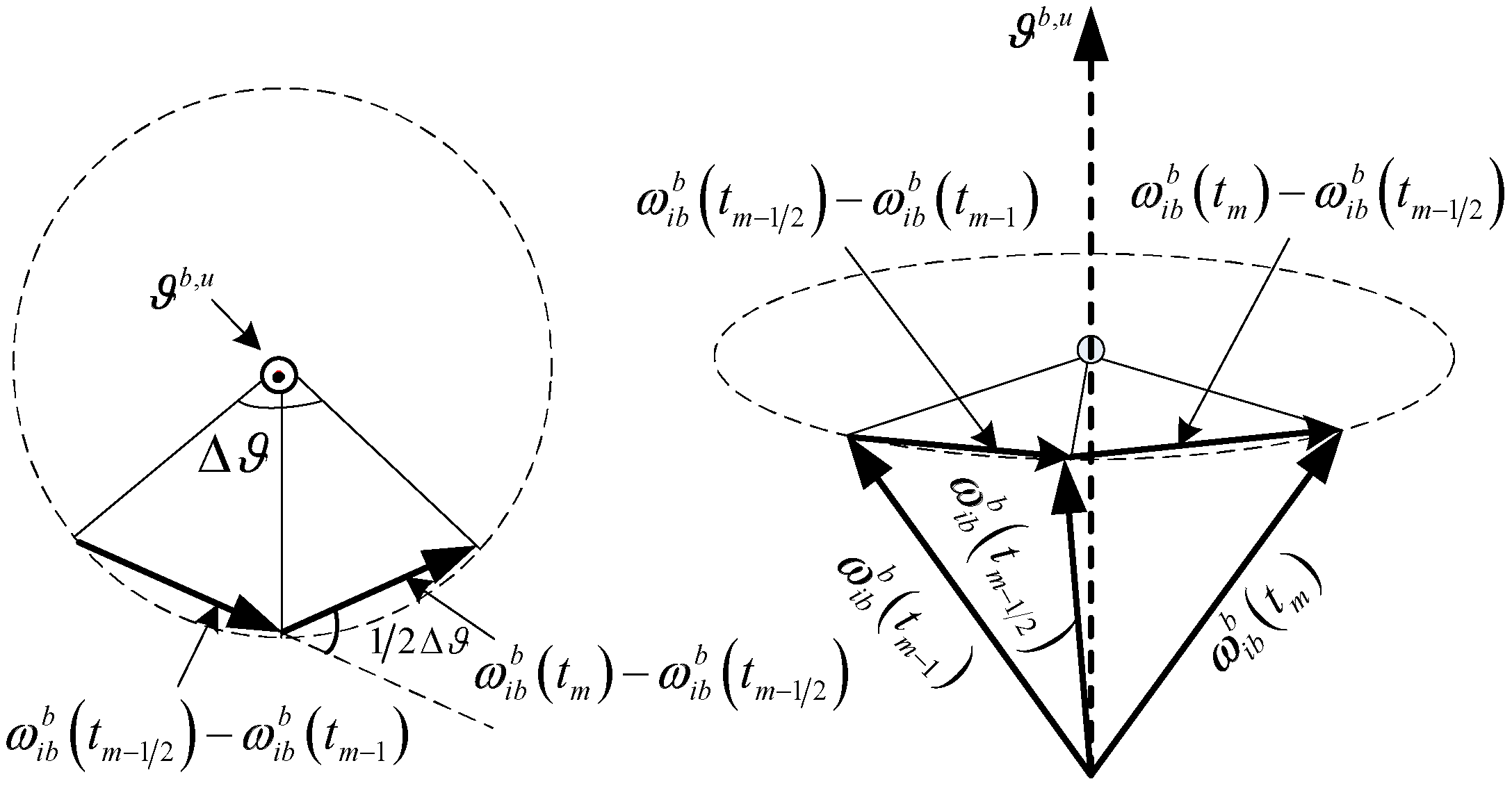
To complete the velocity update using the proposed algorithm, the rotational angular velocity vector ${\vartheta }^{b,u}$ in (21) needs to be determined. ${\vartheta }^{b,u}$ can be computed from the gyroscope’s output angular velocity vectors using a cross-product method, as illustrated in Figure 3. Within the velocity update interval, the angular velocity is sampled consecutively at time $t_{m-1}$, $t_{m-1/2}=t_{m-1}+H/2$ and $t_m=t_{m-1}+H$, yielding ${\omega }_{ib}^b\left(t_{m-1}\right)$, ${\omega }_{ib}^b\left(t_{m-1/2}\right)$, and ${\omega }_{ib}^b\left(t_m\right)$.

Considering that the magnitude of the angular velocity vector remains constant within the $u$ frame, and that the plane formed by vectors ${\omega }_{ib}^b\left(t_{m-1/2}\right)-{\omega }_{ib}^b\left(t_{m-1}\right)$ and ${\omega }_{ib}^b\left(t_m\right)-{\omega }_{ib}^b\left(t_{m-1/2}\right)$ is perpendicular to the rotational angular velocity vector ${\vartheta }^{b,u}$, it follows that vector $\left({\omega }_{ib}^b\left(t_{m-1/2}\right)-{\omega }_{ib}^b\left(t_{m-1}\right)\right)\times \left({\omega }_{ib}^b\left(t_m\right)-{\omega }_{ib}^b\left(t_{m-1/2}\right)\right)$ is co-directional with ${\vartheta }^{b,u}$.

We set

$$e=\left({\omega }_{ib}^b\left(t_{m-1/2}\right)-{\omega }_{ib}^b\left(t_{m-1}\right)\right)\times \left({\omega }_{ib}^b\left(t_m\right)-{\omega }_{ib}^b\left(t_{m-1/2}\right)\right)$$

(24)

The unit vector of the rotational angular velocity vector ${\vartheta }^{b,u}$ can be obtained using

$$e_{\vartheta }={\displaystyle \frac{e}{\left|e\right|}}$$

(25)

Substituting (24) into (25) yields

$$e_{\vartheta }={\displaystyle \frac{\left({\omega }_{ib}^b\left(t_{m-1/2}\right)-{\omega }_{ib}^b\left(t_{m-1}\right)\right)\times \left({\omega }_{ib}^b\left(t_m\right)-{\omega }_{ib}^b\left(t_{m-1/2}\right)\right)}{\left|\left({\omega }_{ib}^b\left(t_{m-1/2}\right)-{\omega }_{ib}^b\left(t_{m-1}\right)\right)\times \left({\omega }_{ib}^b\left(t_m\right)-{\omega }_{ib}^b\left(t_{m-1/2}\right)\right)\right|}}$$

(26)

Based on the principle of the cross product of vectors, the angle between ${\omega }_{ib}^b\left(t_{m-1/2}\right)-{\omega }_{ib}^b\left(t_{m-1}\right)$ and ${\omega }_{ib}^b\left(t_{m-1/2}\right)-{\omega }_{ib}^b\left(t_{m-1}\right)$ is

$$\Delta \vartheta =2{\sin }^{-1}\left({\displaystyle \frac{\left|\left({\omega }_{ib}^b\left(t_{m-1/2}\right)-{\omega }_{ib}^b\left(t_{m-1}\right)\right)\times \left({\omega }_{ib}^b\left(t_m\right)-{\omega }_{ib}^b\left(t_{m-1/2}\right)\right)\right|}{\left|{\omega }_{ib}^b\left(t_{m-1/2}\right)-{\omega }_{ib}^b\left(t_{m-1}\right)\right|·\left|{\omega }_{ib}^b\left(t_m\right)-{\omega }_{ib}^b\left(t_{m-1/2}\right)\right|}}\right)$$

(27)

and the magnitude of the rotational angular velocity vector ${\vartheta }^{b,u}$ can be obtained by

$${\vartheta }^{b,u}={\displaystyle \frac{\Delta \vartheta }{H}}$$

(28)

Substituting (27) into (28) yields

$${\vartheta }^{b,u}={\displaystyle \frac{2}{H}}{\sin }^{-1}\left({\displaystyle \frac{\left|\left({\omega }_{ib}^b\left(t_{m-1/2}\right)-{\omega }_{ib}^b\left(t_{m-1}\right)\right)\times \left({\omega }_{ib}^b\left(t_m\right)-{\omega }_{ib}^b\left(t_{m-1/2}\right)\right)\right|}{\left|{\omega }_{ib}^b\left(t_{m-1/2}\right)-{\omega }_{ib}^b\left(t_{m-1}\right)\right|·\left|{\omega }_{ib}^b\left(t_m\right)-{\omega }_{ib}^b\left(t_{m-1/2}\right)\right|}}\right)$$

(29)

The rotational angular velocity vector ${\vartheta }^{b,u}$ can therefore be expressed in terms of its magnitude ${\vartheta }^{b,u}$ and unit vector $e_{\vartheta }$ as follows [17]:

$${\vartheta }^{b,u}={\vartheta }^{b,u}· e_{\vartheta }$$

(30)

where

$$e_{\vartheta }={\displaystyle \frac{\left({\omega }_{ib}^b\left(t_{m-1/2}\right)-{\omega }_{ib}^b\left(t_{m-1}\right)\right)\times \left({\omega }_{ib}^b\left(t_m\right)-{\omega }_{ib}^b\left(t_{m-1/2}\right)\right)}{\left|\left({\omega }_{ib}^b\left(t_{m-1/2}\right)-{\omega }_{ib}^b\left(t_{m-1}\right)\right)\times \left({\omega }_{ib}^b\left(t_m\right)-{\omega }_{ib}^b\left(t_{m-1/2}\right)\right)\right|}}$$

$${\vartheta }^{b,u}={\displaystyle \frac{2}{H}}{\sin }^{-1}\left({\displaystyle \frac{\left|\left({\omega }_{ib}^b\left(t_{m-1/2}\right)-{\omega }_{ib}^b\left(t_{m-1}\right)\right)\times \left({\omega }_{ib}^b\left(t_m\right)-{\omega }_{ib}^b\left(t_{m-1/2}\right)\right)\right|}{\left|{\omega }_{ib}^b\left(t_{m-1/2}\right)-{\omega }_{ib}^b\left(t_{m-1}\right)\right|·\left|{\omega }_{ib}^b\left(t_m\right)-{\omega }_{ib}^b\left(t_{m-1/2}\right)\right|}}\right)$$

If consecutively sampled angular velocity vectors are constant, i.e., ${\omega }_{ib}^b\left(t_{m-1}\right)={\omega }_{ib}^b\left(t_{m-1/2}\right)={\omega }_{ib}^b\left(t_m\right)$, (30) becomes singular and cannot compute the rotation angular velocity vector ${\vartheta }^{b,u}$. However, Figure 3 demonstrates that in this case it exists that ${\vartheta }^{b,u}=0$. Conversely, if consecutively sampled angular velocities differ, (30) can successfully compute the rotation angular velocity vector ${\vartheta }^{b,u}$.

The next three sampled angular velocity vectors are used to compute ${\vartheta }^{b,u}$ for the subsequent attitude update cycle. This method directly calculates the rotational angular velocity vector via the cross product of angular velocity vectors, offering relatively low computational complexity. It is suitable for scenarios where the velocity update intervals are sufficiently short.

The attitude update algorithm proposed in this study is summarized and listed in

Table 1. Summary of the proposed algorithm.

Inputs: ${\omega }_{ib}^b\left(t_{m-1}\right)$, ${\omega }_{ib}^b\left(t_{m- 1/2}\right)$, ${\omega }_{ib}^b\left(t_m\right)$

Perform the following: Compute rotational angular velocity vector ${\vartheta }^{b,u}$ using the cross product of the sampled angular-rate vectors: $${\vartheta }^{b,u}={\vartheta }^{b,u}· e_{\vartheta }$$ Get the rotation vector ${\varphi }^u(t)$ given ${\omega }_{ib}^b\left(t_{m-1}\right)$ and ${\vartheta }^{b,u}$ $${\varphi }^{iu}(t)={\displaystyle {\int }_{t_{m-1}}^t\left({\omega }_{ib}^b\left(t_{m-1}\right)+{\vartheta }^{b,u}\right)}\mathrm{d}\tau$$ Get the rotation vector ${\varphi }^{ub}(t)$ given ${\vartheta }^{b,u}$ $${\varphi }^{ub}(t)={\displaystyle {\int }_{t_{m-1}}^t\left(-{\vartheta }^{b,u}\right)}\mathrm{d}\tau$$ Compute the transformation matrix $C_{i m-1}^u$. $$C_{i m-1}^u=I+{\displaystyle \frac{\sin {\varphi }^{iu}\left(t\right)}{{\varphi }^{iu}\left(t\right)}}\left({\varphi }^{iu}\left(t\right)\times \right)+{\displaystyle \frac{1-\cos {\varphi }^{iu}\left(t\right)}{{\varphi }^{iu}{\left(t\right)}^2}}{\left({\varphi }^{iu}\left(t\right)\times \right)}^2$$ Get the transformation matrix $C_{u m-1}^b$ $$C_{u m-1}^b=I+{\displaystyle \frac{\sin {\varphi }^{ub}\left(t\right)}{{\varphi }^{ub}\left(t\right)}}\left({\varphi }^{ub}\left(t\right)\times \right)+{\displaystyle \frac{1-\cos {\varphi }^{ub}\left(t\right)}{{\varphi }^{ub}{\left(t\right)}^2}}{\left({\varphi }^{ub}\left(t\right)\times \right)}^2$$ Compute the transformation matrix $C_{i m-1}^b$ $$C_{i m-1}^b=C_{u m-1}^b{C}_{i m-1}^u$$ Obtain the transformation matrix at $t_m$: $C_i^b(t_m)=C_{i 1}^b{C}_{i 2}^b{C}_{i 3}^b\cdots C_{i m-1}^b$

Output: $C_i^b(t_m)$

to facilitate better execution in the navigation computer.

4. Algorithm’s Performance Under Low-Dynamic Motion

In low-dynamic motion, the angular velocity ${\omega }_{ib}^b\left(t\right)$ typically exhibits smooth variations, which can be mathematically approximated as a polynomial function of time [7]. Within attitude update cycle $H=t_m-t_{m-1}$, the angular velocity ${\omega }_{ib}^b\left(t\right)$ is modeled as a second-order polynomial:

$${\omega }_{ib}^b\left(t\right)=a+b\left(t-t_{m-1}\right)+c{\left(t-t_{m-1}\right)}^2$$

(31)

where $a,b,c$ are constant vectors.

Let

$$a=\left[\begin{array}{c}{a}_1\\ a_2\\ a_3\end{array}\right],b=\left[\begin{array}{c}{b}_1\\ b_2\\ b_3\end{array}\right],c=\left[\begin{array}{c}{c}_1\\ c_2\\ c_3\end{array}\right]$$

(32)

Three equidistant angular velocity vectors ${\omega }_{ib}^b\left(t_0\right),{\omega }_{ib}^b\left(t_1\right),{\omega }_{ib}^b\left(t_2\right)$ are sampled within the attitude update cycle $H=t_m-t_{m-1}$, where $t_1=t_0+h,t_2=t_0+2h$.

The angular velocity vectors under low-dynamic motion can be expressed as

$$\begin{array}{l}{\omega }_{ib}^b\left(t_0\right)=a,\\ {\omega }_{ib}^b\left(t_1\right)=a+bh+c{h}^2\\ {\omega }_{ib}^b\left(t_2\right)=a+2bh+4c{h}^2\end{array}$$

(33)

The relationship between the algorithm error and low-dynamic motion parameters is described in detail in the Appendix A. The algorithm’s performance under low-dynamic motion reduces to a functional relationship $\Delta Err=f\left(a,b,c,h,h^2,h^3\right)$. The attitude error is influenced by the values of $a,b,c,$ and is also dependent on the size of the attitude update cycle.

The algorithm error $\Delta Err$ vanishes for two special conditions in (31). One is a piecewise constant scenario; the other one is the limit as H → 0. A comprehensive performance evaluation against low-dynamic motion is presented in Section 5.

5. Simulations and Discussion

Simulations are carried out using MATLAB R2016b to numerically verify the accuracy of the proposed attitude algorithm. The proposed attitude algorithm (Prop) is evaluated to validate its performance under low-dynamic motion, as described in (31). The comparison algorithms are the traditional algorithm (Trad1), as described in Section 2, and a muti-interval information algorithm (Trad2), as described in [15]:

$$\begin{array}{l}\stackrel{⌢}{\beta }=\alpha +H^2\left(-0.1662{\omega }_1\times {\omega }_2+0.0052{\omega }_0\times {\omega }_2\right)\\ \hspace{1em} +0.6926{\alpha }_1\times {\alpha }_2+H\left(0.4390{\omega }_1\times {\alpha }_2-0.0597{\omega }_2\times {\alpha }_2\right)\end{array}$$

(34)

where $\alpha ={\displaystyle \frac{H}{6}}({\omega }_0+4{\omega }_1+{\omega }_2),{\alpha }_1={\displaystyle \frac{H}{3}}{\omega }_1,{\alpha }_2={\displaystyle \frac{H}{3}}{\omega }_2$, $H=2h$.

As in the error analysis in Section 4, the algorithm error depends on the parameters of the low-dynamic motion.

Table 2. Simulation parameters under low-dynamic motion.

Conditions	$\mathit{a}\left(\mathbf{rad}/\mathbf{s}\right)$	$\mathit{b}\left(\mathbf{rad}/{\mathbf{s}}^{\mathbf{2}}\right)$	$\mathit{c}\left(\mathbf{rad}/{\mathbf{s}}^{\mathbf{3}}\right)$	$\mathit{H}\left(\mathbf{s}\right)$
Case 1	${\left[\begin{array}{ccc}1& 0& 0\end{array}\right]}^{\mathrm{T}}$	${\left[\begin{array}{ccc}0& 1& 0\end{array}\right]}^{\mathrm{T}}$	${\left[\begin{array}{ccc}0& 0& 1\end{array}\right]}^{\mathrm{T}}$	0.01
Case 2	${\left[\begin{array}{ccc}2& 0& 0\end{array}\right]}^{\mathrm{T}}$	${\left[\begin{array}{ccc}0& 1& 0\end{array}\right]}^{\mathrm{T}}$	${\left[\begin{array}{ccc}0& 0& 1\end{array}\right]}^{\mathrm{T}}$	0.01
Case 3	${\left[\begin{array}{ccc}1& 0& 0\end{array}\right]}^{\mathrm{T}}$	${\left[\begin{array}{ccc}0& 2& 0\end{array}\right]}^{\mathrm{T}}$	${\left[\begin{array}{ccc}0& 0& 1\end{array}\right]}^{\mathrm{T}}$	0.01
Case 4	${\left[\begin{array}{ccc}1& 0& 0\end{array}\right]}^{\mathrm{T}}$	${\left[\begin{array}{ccc}0& 1& 0\end{array}\right]}^{\mathrm{T}}$	${\left[\begin{array}{ccc}0& 0& 2\end{array}\right]}^{\mathrm{T}}$	0.01
Case 5	${\left[\begin{array}{ccc}1& 0& 0\end{array}\right]}^{\mathrm{T}}$	${\left[\begin{array}{ccc}0& 1& 0\end{array}\right]}^{\mathrm{T}}$	${\left[\begin{array}{ccc}0& 0& 1\end{array}\right]}^{\mathrm{T}}$	0.02

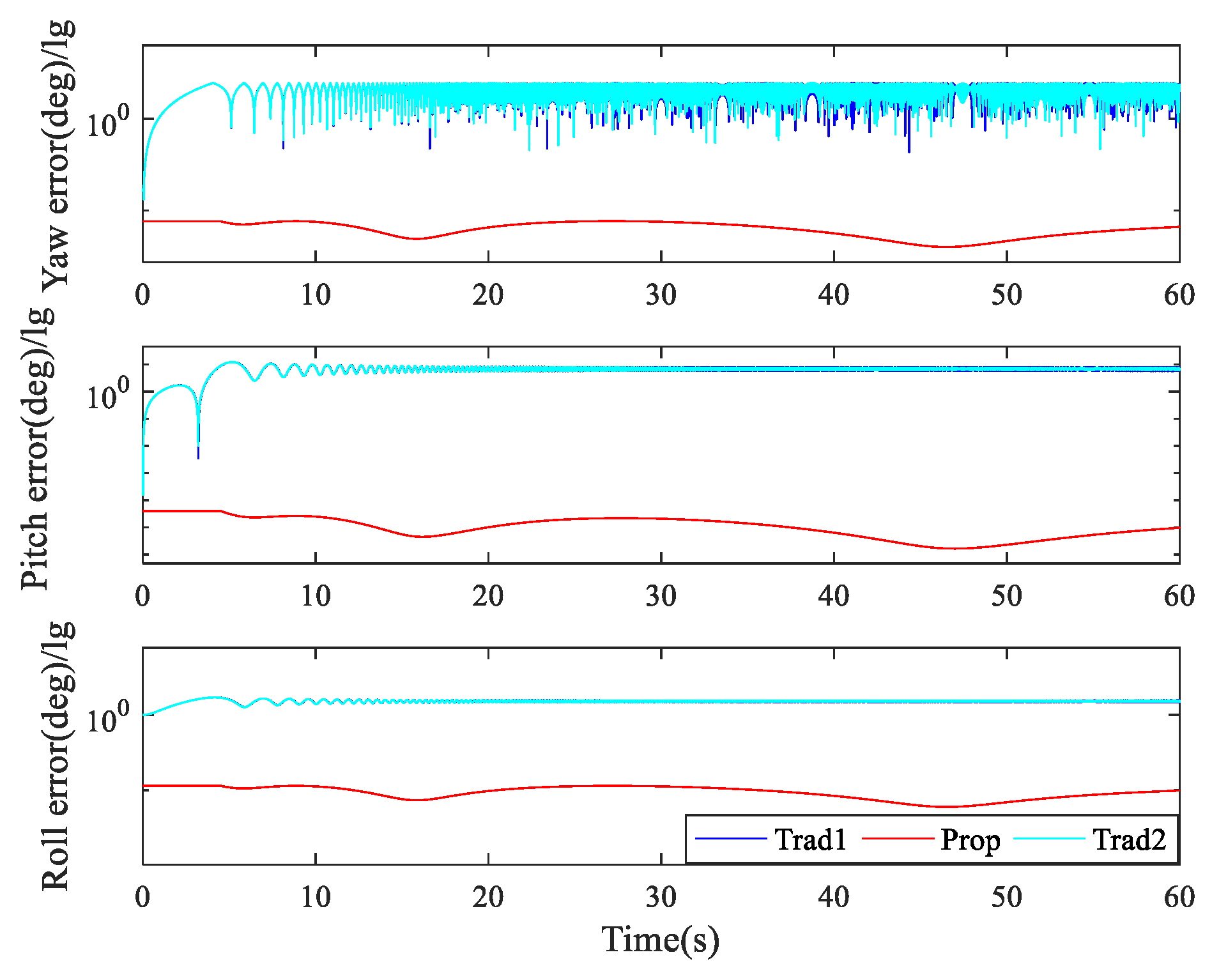
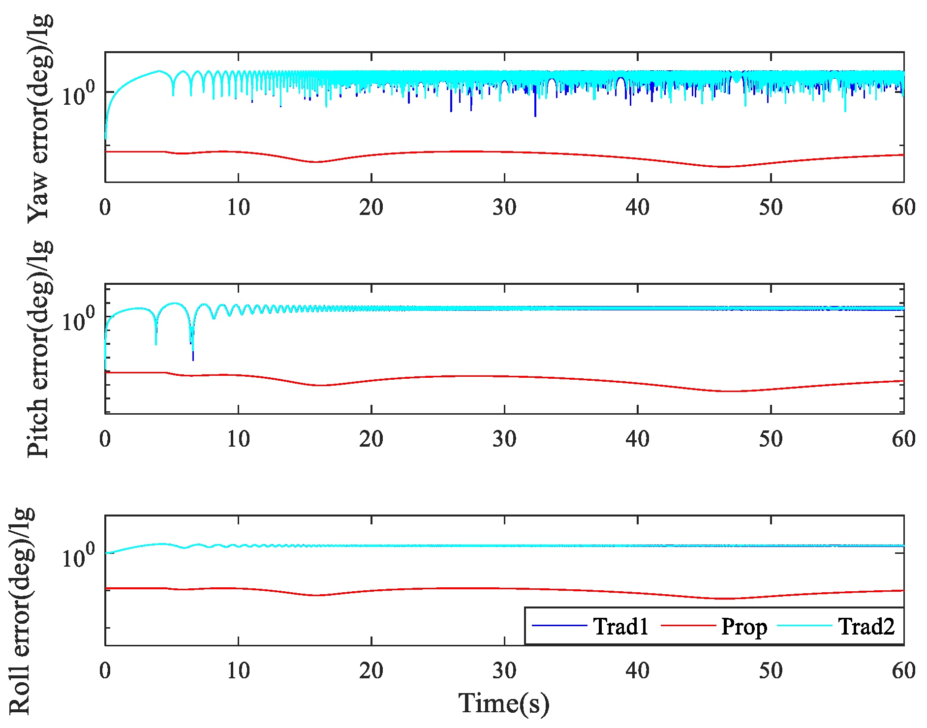
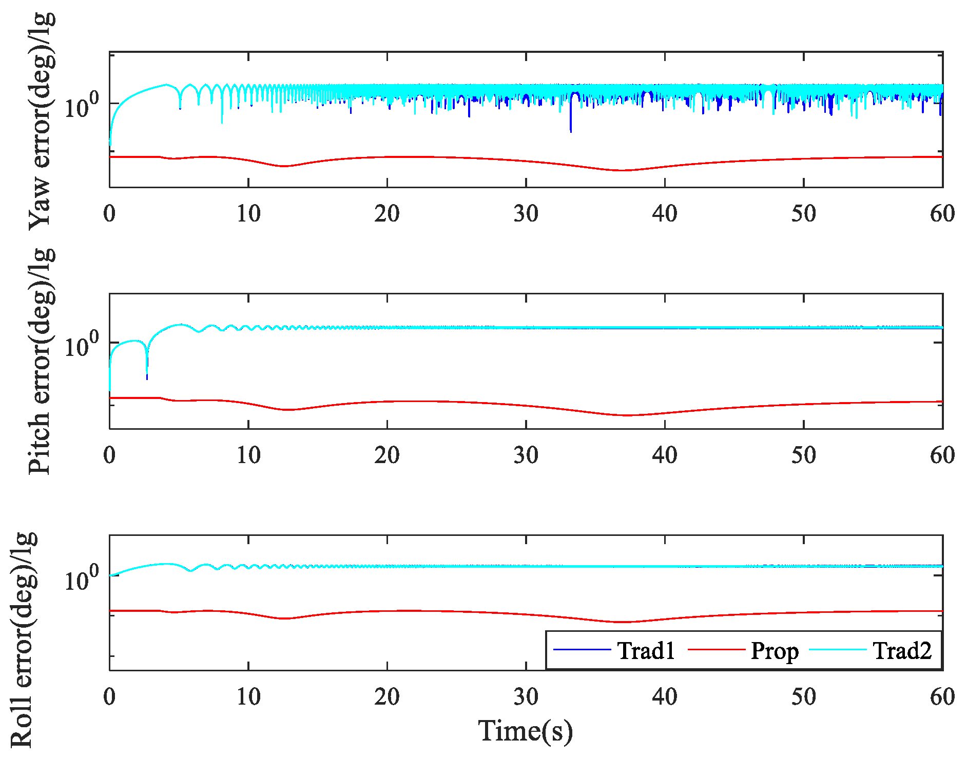
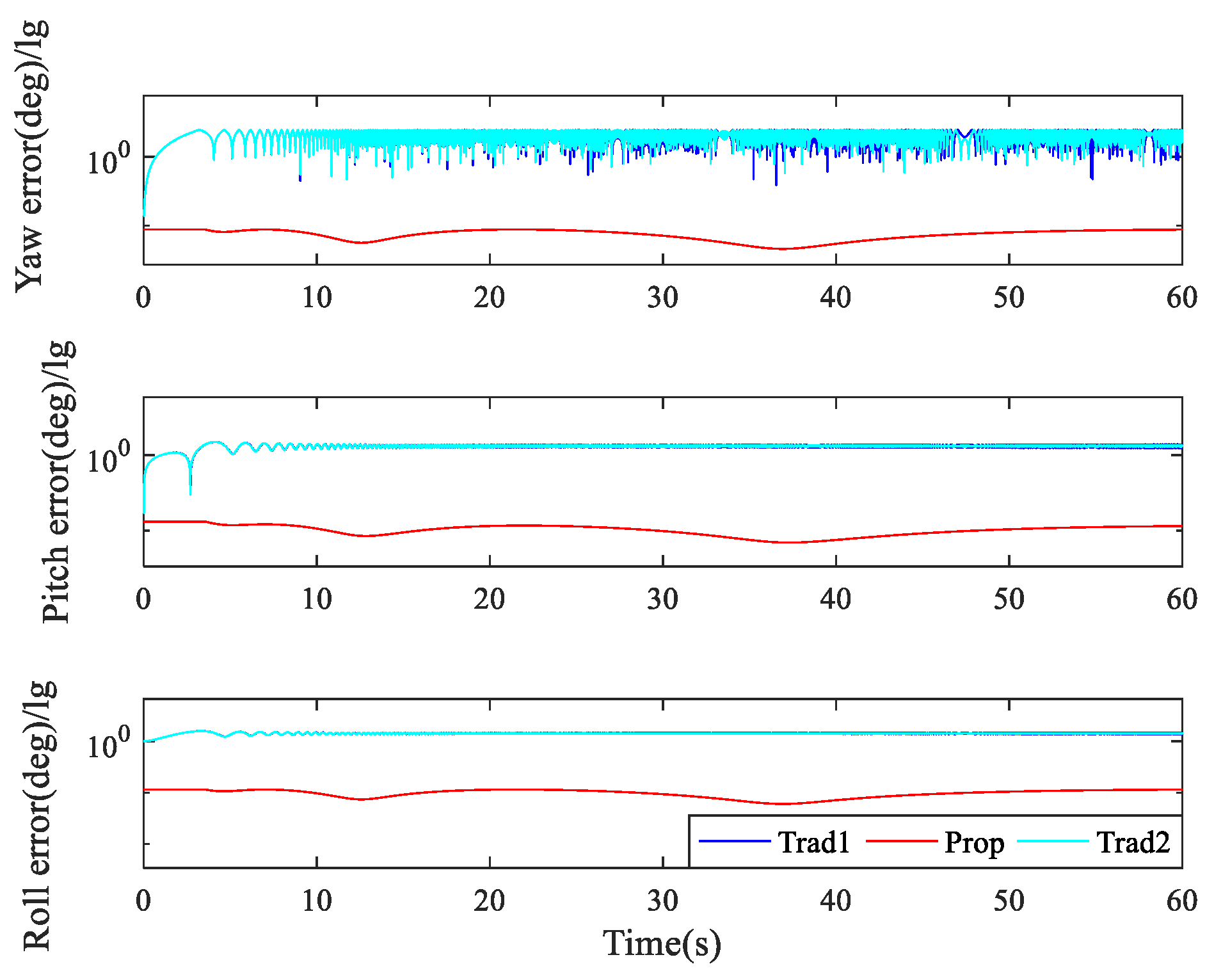
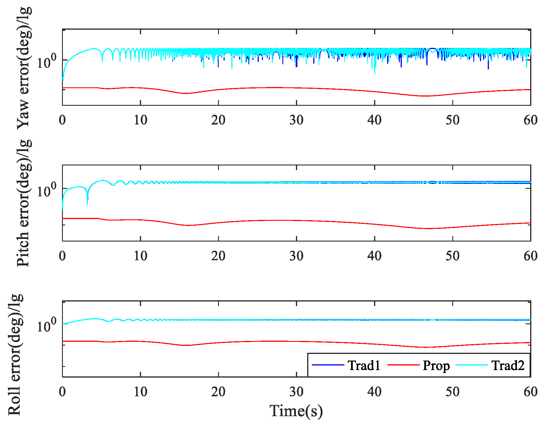
$a$ represents the variation in initial angular velocity; $b$ represents the variation in initial angular acceleration; $c$ represents the variation in the rate of change in angular acceleration.

lists the simulation parameters under low-dynamic motion. The simulation results are represented in Figure 4, Figure 5, Figure 6, Figure 7 and Figure 8.

Table 3. Algorithm errors of each case under low-dynamic motion.

Conditions	Error	Trad1 Maximum (deg)	Trad2 Maximum (deg)	Prop Maximum (deg)
Case 1	Yaw	89.99	89.98	$2.6\times {10}^{-6}$
	Pitch	12.2	12.17	$4.0\times {10}^{-5}$
	Roll	14.45	14.38	$2.0\times {10}^{-5}$
Case 2	Yaw	89.99	89.99	$2.6\times {10}^{-6}$
	Pitch	9.465	9.463	$8.0\times {10}^{-5}$
	Roll	15.88	15.82	$2.0\times {10}^{-5}$
Case 3	Yaw	89.99	89.98	$2.6\times {10}^{-6}$
	Pitch	26.92	26.85	$4.0\times {10}^{-5}$
	Roll	26.63	26.47	$4.0\times {10}^{-5}$
Case 4	Yaw	90	89.98	$5.3\times {10}^{-6}$
	Pitch	7.242	7.226	$4.0\times {10}^{-5}$
	Roll	9.72	9.661	$4.0\times {10}^{-5}$
Case 5	Yaw	89.97	89.98	$2.1\times {10}^{-5}$
	Pitch	12.2	12.14	$8.0\times {10}^{-5}$
	Roll	14.49	14.34	$8.0\times {10}^{-5}$

provides a comprehensive quantitative comparison of algorithm errors.

In case 2, the increase in parameter $a$, which the parameter sets aim to represent, corresponds to a slight offset in the initial rotational state of the object, i.e., changing from nearly stationary to extremely slow rotation. In case 3, the increase in parameter $b$, which the parameter sets aim to represent, corresponds to a faint change in the initial trend of rotational acceleration, i.e., shifting from completely uniform motion to an extremely gradual increase in speed. In case 4, the increase in parameter $c$, which the parameter sets aim to represent, corresponds to an upward bend in the angular velocity curve of the object’s motion, meaning that it accelerates more and more rapidly.

Figure 4, Figure 5, Figure 6, Figure 7 and Figure 8 show that under all five cases, the yaw, pitch, and roll error curves of Prop are consistently lower than those of Trad1 and Trad2. Analysis of Table 3 further reveals the following: when increasing low-dynamic parameter $a$ (case 2), the maximum yaw error of Trad1 and Trad2 remained unchanged, its maximum pitch error decreased, and its maximum roll error increased. For Prop, the maximum yaw and roll errors remained unchanged, while its maximum pitch error increased. With increased low-dynamic parameter $b$ (case 3), the maximum roll and pitch errors of Trad1 and Trad2 increased, while their maximum yaw error remained unchanged. The maximum yaw and pitch errors of Prop remained unchanged, but its maximum roll error increased. Under increased low-dynamic parameter $c$ (case 4), the maximum yaw error of Trad1 and Trad2 remained unchanged, while their maximum pitch and roll errors decreased. The maximum pitch and roll errors of Prop remained unchanged, but its maximum yaw error increased. With increased low-dynamic parameter $H$ (case 5), the maximum yaw, pitch, and roll errors of Trad1 and Trad2 all remained unchanged. The maximum yaw, pitch, and roll errors of Prop all increased. Comparing the maximum errors of Trad1 and Trad2 under five cases shows that the yaw error is the largest among the three, significantly exceeding both the pitch and roll errors. In contrast, the maximum errors of Prop vary with changes in low-dynamic parameters; they all remain within the order of magnitude of ${10}^{-5}$ across all five cases. It is significantly lower than the three-axis errors of Trad1 and Trad2. This validates the effectiveness of Prop in low-dynamic motion and aligns with the error analysis results in Section 4.

A comparative analysis of algorithm accuracy and computational cost between the proposed algorithm and traditional ones is necessary. The single-update execution time of algorithms was quantified by employing tic and toc functions in MATLAB R2016b.

As shown in

Table 4. Single-update execution time of algorithms.

Algorithm Time	Trad1 (s)	Trad2 (s)	Prop (s)
Case 1	$1.8\times {10}^{-5}$	$2.8\times {10}^{-5}$	$5.5\times {10}^{-5}$
Case 2	$2.3\times {10}^{-5}$	$2.8\times {10}^{-5}$	$5.3\times {10}^{-5}$
Case 3	$2.0\times {10}^{-5}$	$2.8\times {10}^{-5}$	$5.3\times {10}^{-5}$
Case 4	$2.2\times {10}^{-5}$	$3.3\times {10}^{-5}$	$5.5\times {10}^{-5}$
Case 5	$3.0\times {10}^{-5}$	$3.3\times {10}^{-5}$	$6.6\times {10}^{-5}$

, under all five cases, Trad1 has the smallest time consumption, followed by Trad2, and Prop has the largest. Combined with the algorithm accuracy analysis, it can be concluded that Prop outperforms Trad1 and Trad2 in terms of accuracy and it incurs a higher computational cost. Despite this, its execution time still satisfies the constraint of being less than 70% of the algorithm update cycle [22].

6. Conclusions

To enhance the accuracy of attitude update algorithms under low-dynamic motion, this paper proposes a novel symmetry-based attitude update method. It systematically evaluates the applicability of the algorithm under this motion. The performance of the proposed algorithm under low-dynamic motion was sufficiently compared with that of the traditional ones in the simulation. Simulation results demonstrate that the proposed algorithm outperforms traditional algorithms.