Research on Microgrid Dispatch Management Method Based on Improved Enterprise Development Optimization Algorithm

Abstract

Metaheuristic optimization algorithms often suffer from structural imbalance between exploration and exploitation, leading to premature convergence and performance degradation in high-dimensional or constrained problems. To address this issue, a symmetry-enhanced Improved Enterprise Development Optimization Algorithm (IEDOA) is proposed. The algorithm establishes a dynamic symmetry between global exploration and local exploitation through three coordinated strategies: a performance-feedback-based adaptive activity selection mechanism, a multi-elite-guided structural evolution strategy, and a lifecycle-aware exploration mechanism inspired by technological scheduling dynamics. The proposed symmetric regulation framework improves population diversity while preserving convergence stability, thereby enhancing search efficiency in complex landscapes. To validate its performance, IEDOA is evaluated on CEC2017 (30/50 dimensions) and CEC2022 (10/20 dimensions) benchmark suites and compared with several advanced metaheuristic algorithms. Experimental results demonstrate superior convergence accuracy, robustness, and scalability. Statistical analyses using the Wilcoxon signed-rank and Friedman tests further confirm its significant performance advantages. To demonstrate practical applicability, IEDOA is applied to a grid-connected microgrid economic dispatch problem involving renewable generation units, controllable generators, and energy storage systems under 24 h operational constraints. Simulation results show that the proposed method achieves lower operational costs and smaller performance variance across independent runs. Overall, IEDOA provides an effective symmetric optimization framework for complex engineering systems characterized by nonlinearity, multi-constraints, and high dimensionality.

1. Introduction

With the rapid development of renewable energy technologies and the continuous advancement of energy structure transformation, microgrids, as local energy systems integrating distributed power sources, energy storage systems, and loads, have attracted widespread attention from academia and engineering circles due to their significant advantages in improving energy utilization efficiency, enhancing power supply reliability, and promoting the integration of renewable energy. Microgrids typically include various energy units such as photovoltaic systems, wind turbines, diesel generators, and energy storage devices. Their operating status is affected by multiple factors, including the randomness of renewable energy output, load fluctuations, and operational constraints, resulting in highly nonlinear, multi-constrained, and multi-objective complex characteristics in microgrid scheduling and management problems [1,2,3].

The core objectives of microgrid dispatch and management are to minimize operating costs, maximize energy utilization efficiency, and optimize environmental benefits, all while ensuring the safe and stable operation of the system [4,5]. Traditional scheduling methods are mainly based on deterministic models or linear optimization techniques, such as mixed-integer linear programming [6,7] and dynamic programming [8,9]. While these methods can achieve good optimization results for smaller models or simpler system structures, they often suffer from high computational complexity, low solution efficiency, and a tendency to get stuck in local optima when dealing with microgrid systems containing a large number of distributed energy resources and complex operational constraints. This makes it difficult to meet the real-time and robustness requirements of practical engineering applications [10,11,12].

In recent years, heuristic algorithms have been widely applied in various fields due to their excellent global search capabilities and strong adaptability. For example, in the field of unmanned aerial vehicle (UAV) path planning, Li et al. proposed a novel hybrid particle swarm optimization algorithm by combining simulated annealing and particle swarm optimization algorithms to plan UAV paths in complex three-dimensional environments. Experimental results showed that the SDPSO algorithm can quickly plan higher-quality UAV paths [13]. Nandhini Kullampalayam Murugaiyan et al. proposed an improved PV parameter extraction algorithm using an opposition-based exponential distribution optimizer (OBEDO). In experiments with single-diode, double-diode, triple-diode, and photovoltaic module models, OBEDO demonstrated advantages in computational efficiency and robustness, making it a promising solution for photovoltaic model parameter identification and contributing significantly to improving photovoltaic system performance [14]. In medical imaging, Yusuf Uzun et al. developed a non-elitist WSO algorithm that improved contrast by 15% and entropy by 10% in MRI images, resulting in clearer image details and significantly improving the accuracy of doctors’ disease diagnosis [15]. The field of microgrid dispatching is no exception. Feng et al. proposed a novel adaptive robust multi-objective optimization algorithm by evaluating the evolutionary state of the population for adaptive selection. This algorithm was then applied to microgrid dispatching optimization. Experimental results show that the proposed method achieves good results in solving microgrid dispatching problems [16]. Inspired by different life stages of wild geese, Vimal Tiwari et al. developed a wild geese algorithm. Experimental results show that optimized scheduling using the Wild Geese Algorithm (WGA) can effectively reduce the operating costs of the power grid [17].

The Enterprise Development Optimization Algorithm (EDOA), proposed by Dinh-Nhat Truong et al. in 2024, is a novel metaheuristic optimization algorithm designed specifically for advanced engineering solutions, inspired by enterprise development. Its application to global optimization and optimal design of structures yielded significant results, promoting the application of metaheuristic algorithms in structural engineering simulation. Since its inception, it has been widely used in various fields [18]. For example, Zhao et al. proposed LMEDOA by integrating a time-phase-based switching strategy, an economy-driven guided learning strategy, and a spatially selective selection strategy into EDOA to solve numerical optimization and engineering design optimization problems. Experiments on the CEC2018 test set and engineering design optimization problems show that LMEDOA is a promising variant of EDOA, which is both effective and accurate in solving complex problems [19]. To address engineering constraint problems, Cai et al. proposed an improved EDOA (Effective Optimization Problem) strategy based on leader covariance learning. Experimental results from CEC2017 and CEC2022 demonstrate that MSEDOA, with its effective utilization and exploration capabilities, can effectively escape local optima. Experimental results on ten engineering constraint problems show that MSEDO is capable of solving complex real-world optimization problems [20]. To address the Photovoltaic Model Parameter Estimation problem, Li et al. proposed a Multi-Policy Enhanced Enterprise Development (MEED) optimization algorithm that combines chaotic mapping and adversarial learning for initialization. Experimental results show that MEED provides an efficient and reliable optimization framework for PV model parameter estimation and other complex engineering optimization problems [21].

As the No Free Lunch theorem states, no single algorithm performs well on all problems. Therefore, specific problems require targeted improvements to enhance the algorithm’s performance. To address the microgrid scheduling problem, based on the above research, this paper proposes an Improved Enterprise Development Optimization Algorithm (IEDOA), with the following specific contributions:

• To address the shortcomings of the original EDOA (Enterprise Development Optimization Algorithm), such as convergence instability and difficulty in balancing exploration and exploitation in complex optimization problems, an improved Enterprise Development Optimization Algorithm (IEDOA) is proposed to enhance the overall solution performance of the algorithm in complex search spaces.
• We propose a performance-feedback-based adaptive activity selection strategy, which dynamically adjusts the selection probabilities of different activity mechanisms. This allows the algorithm to adaptively allocate search resources based on search performance, thereby improving convergence efficiency and stability.
• A multi-elite-guided structural evolution strategy is proposed, which guides the population structure update by introducing elite information, thereby enhancing the inheritance ability of high-quality solutions and improving the optimization accuracy and robustness of the algorithm on complex functions.
• A technology lifecycle-aware search scheduling mechanism is proposed, which adaptively adjusts the intensity of exploration and exploitation according to the iteration stage. This allows the algorithm to maintain stronger global search capabilities in the early stages and stronger local exploitation capabilities in the later stages, thereby reducing the risk of getting trapped in local optima.
• Through comparative experiments using the CEC2017 and CEC2022 benchmark tests and statistical analysis, the proposed IEDOA was verified to have superior optimization performance and stronger stability under different dimensional settings, demonstrating good adaptability and scalability. Furthermore, experimental analysis in microgrid scheduling optimization showed that IEDOA has good practical applicability.

This paper is organized into six sections. Section 2 presents an overview of EDOA. In Section 3, a targeted improvement strategy for microgrid scheduling is developed. Section 4 conducts comparative evaluations with several optimization algorithms based on the CEC2017 and CEC2022 benchmark problems. Section 5 investigates the application of IEDOA to a practical microgrid scheduling task to assess its engineering performance. Section 6 concludes the study and discusses possible avenues for future work.

2. Enterprise Development Optimization Algorithm (EDOA)

The EDOA is inspired by Leavitt’s more than 20 years of research on industrial organizations, which shows that complex organizational systems depend on the interaction between tasks, structure, technology, and people. Tasks refer to the organization’s primary goals in manufacturing or service, usually composed of multiple subtasks that have practical operational significance in complex organizations. Structure refers to the internal communication system, allocation of responsibilities (or roles), and workflows within the organization. Technology refers to the tools, equipment, and methods used to accomplish tasks and facilitate organizational operations. People refer to individuals, but their behavior is not limited to the human realm and may exhibit different characteristics at different times or in different environments. The specific optimization process is as follows:

2.1. Population Initialization

Similar to all metaheuristic optimization algorithms, the EDOA first generates an initial population using a uniform random distribution. In the first iteration, the initial population is obtained through Equation (1).

$$X_i=lb+(ub-lb)\times rand\left(\mathrm{0,1}\right),$$

(1)

where $X_i$ is the $i$-th individual of the population, $lb$ and $ub$ are the lower and upper bounds of the problem, respectively, and $rand\left(\mathrm{0,1}\right)$ is a uniformly distributed random number in $[0,1]$.

2.2. Establishing Optimal Rules and Simulation Activities

The algorithm simulates the enterprise development process through four types of activities: tasks, structure, technology, and personnel, and introduces an activity switching mechanism to dynamically transition between different activities. The solutions generated by these activities are closely related to organizational performance, with more attractive solutions corresponding to higher performance. Ultimately, the algorithm quantifies organizational performance through the solutions and their corresponding objective function values, thereby evaluating the quality of the solutions and guiding the optimization process. Specific details are as follows:

2.2.1. Task

In business process management, tasks can appear in different forms or function as routine operational activities. In the EDOA, task-related activities are simulated by replacing the worst-performing individual in the population. This operation is mathematically described by Equation (2):

$$X_{\mathrm{w}orst}\left(\mathrm{t}\right)=lb+\left(ub-lb\right)\times rand\left(\mathrm{0,1}\right),$$

(2)

where $X_{\mathrm{w}orst}\left(\mathrm{t}\right)$ represents the individual with the poorest performance in the population at iteration $\mathrm{t}$.

2.2.2. Structure

Previous studies on organizational design for human efficiency indicate that modifying work arrangements from a social engineering perspective can significantly affect individual behavior and performance outcomes. In the EDOA, organizational structure is simplified and represented in terms of workflows. When a new structure is generated, it is assumed to be jointly influenced by both the current best-performing workflow and other existing workflows within the organization. Accordingly, the structural update mechanism is formulated as

$$X_i^s\left(\mathrm{t}\right)=X_i^s\left(\mathrm{t}-1\right)+rand\left(-\mathrm{1,1}\right)\times \left(X_{best}\left(\mathrm{t}-1\right)-X_c^s\left(\mathrm{t}-1\right)\right),$$

(3)

where $X_i^s\left(\mathrm{t}\right)$ represents the updated organizational structure at iteration $\mathrm{t}$, and $X_i^s\left(\mathrm{t}-1\right)$ denotes its previous state. The term $X_{best}\left(\mathrm{t}-1\right)$ refers to the best solution identified in the preceding iteration, while $X_c^s\left(\mathrm{t}-1\right)$ corresponds to the centroid of other workflows that exert influence on the new structure. The random coefficient $rand\left(-\mathrm{1,1}\right)$ is a uniformly distributed random number in the interval $[-\mathrm{1,1}]$.

The centroid of the influencing workflows is computed as

$$X_c^s\left(\mathrm{t}-1\right)={\displaystyle \frac{X_{{rand}_1}^s\left(\mathrm{t}-1\right)+X_{{rand}_2}^s\left(\mathrm{t}-1\right)+\dots +X_{{rand}_m}^s\left(\mathrm{t}-1\right)}{m}},$$

(4)

where $m$ denotes the number of workflows considered in the structural interaction and is set to 3 in this study. The terms $X_{{rand}_1}^s\left(\mathrm{t}-1\right)$, $X_{{rand}_2}^s$,…, $X_{{rand}_m}^s\left(\mathrm{t}-1\right)$ are solutions randomly selected from the current population.

2.2.3. Technology

Technological capability is a key driver of organizational transformation, as many structural and strategic changes are triggered by advances in technology rather than by abstract ideas alone. From the perspective of open innovation, external knowledge inputs mainly support an organization’s ability to explore new solutions, whereas innovation outputs are more strongly associated with the effective utilization and refinement of existing knowledge and technological foundations. Consequently, organizations are required to simultaneously strengthen exploratory and exploitative behaviors in order to acquire, integrate, and apply knowledge in support of innovation.

Within the EDOA, the interaction between exploration and exploitation during the technology phase is modeled through a combined update strategy. The technological state of each solution is updated according to

$$\begin{array}{c}{X}_i^{\tau }\left(\mathrm{t}\right)=X_i^{\tau }\left(\mathrm{t}-1\right)+{rand}^{\alpha }\left(\mathrm{0,1}\right)\times \left(X_{best}\left(\mathrm{t}-1\right)-X_i^{\tau }\left(\mathrm{t}-1\right)\right)\\ +{rand}^{\beta }\left(\mathrm{0,1}\right)\times \left(X_{best}\left(\mathrm{t}-1\right)-X_{{rand}_1}^{\tau }\left(\mathrm{t}-1\right)\right)\end{array},$$

(5)

where the first update term reflects exploitation, guiding the solution toward the current best-performing state, while the second term promotes exploration by incorporating information from a randomly selected solution in the population. The coefficients ${rand}^{\alpha }\left(\mathrm{0,1}\right)$ and ${rand}^{\beta }\left(\mathrm{0,1}\right)$ are independent random numbers in the interval $\left[\mathrm{0,1}\right]$, controlling the relative influence of exploitation and exploration during the technological evolution process.

2.2.4. People

An effective organization requires a collaborative working environment that values individual participation and collective effort. By encouraging cooperation and recognizing the influence of interpersonal interactions, organizations can enhance creativity, engagement, and overall performance. In the EDOA, people-related activities are represented by updating individual characteristics through interactions with influential peers, thereby capturing the social dynamics within the organization.

The update mechanism for the people component is defined as

$$X_{i,d}^p\left(\mathrm{t}\right)=X_{i,d}^p\left(\mathrm{t}-1\right)+rand\left(-\mathrm{1,1}\right)\times \left(X_{best,d}\left(\mathrm{t}-1\right)-X_{c,d}^p\left(\mathrm{t}-1\right)\right),$$

(6)

where $X_{i,d}^p\left(\mathrm{t}\right)$ denotes the updated value of the $d$-th characteristic of individual $i$ at iteration $t$. The term $X_{c,d}^p\left(\mathrm{t}-1\right)$ represents the average influence exerted by other individuals and is computed as

$$X_{c,d}^p\left(\mathrm{t}-1\right)={\displaystyle \frac{X_{{rand}_1,d}^p\left(\mathrm{t}-1\right)+X_{{rand}_2}^s\left(\mathrm{t}-1\right)+\dots +X_{{rand}_m}^s\left(\mathrm{t}-1\right)}{m}},$$

(7)

where $m$ is the number of individuals contributing to the interaction and is set to 3 in this study. The variables $X_{{rand}_1,d}^p\left(\mathrm{t}-1\right)$, $X_{{rand}_2}^s\left(\mathrm{t}-1\right)$,…, $X_{{rand}_m}^s\left(\mathrm{t}-1\right)$ are randomly selected from the population.

The dimension $d$ is randomly chosen to represent a specific individual characteristic and is determined by

$$d=⌈rand\left(\mathrm{0,1}\right)\times n_d⌉,$$

(8)

where $n_d$ denotes the dimensionality of the solution space.

2.3. Mechanism of Switching Activities

In the EDOA, it is assumed that an organization concentrates on a single developmental activity at each iteration. As a result, only one of the four activities—task, structure, technology, or people—is executed at time step $t$. The selection of the active process is governed by an activity-switching mechanism, which dynamically determines the operational focus during the optimization process.

This mechanism is controlled by a time-dependent function $C\left(t\right)$, defined as

$$C\left(t\right)=⌈3\times \left(1-{\displaystyle \frac{rand\left(\mathrm{0,1}\right)\times t}{T}}\right)⌉,$$

(9)

where $t$ denotes the current iteration index, and $T$ represents the maximum number of iterations. The value of $C\left(t\right)$ determines which activity is selected, allowing the algorithm to adaptively shift its emphasis as the search progresses.

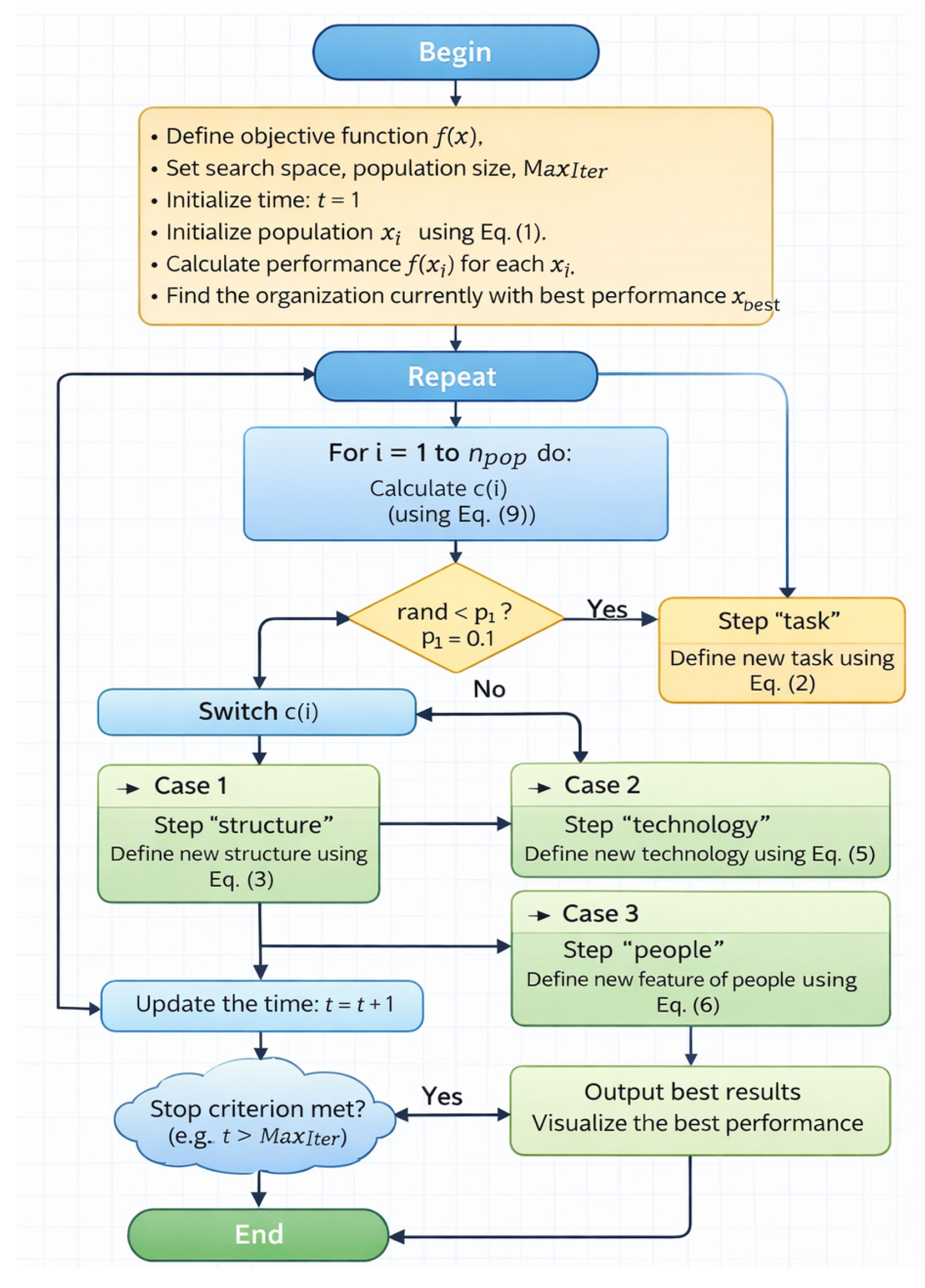
In addition, a small probability $p_1= 0.1$ is introduced to explicitly trigger the task-related activity, ensuring sufficient diversity during the search. The overall decision logic of the activity selection procedure is summarized in Algorithm 1. Figure 1 illustrates the specific process of EDOA.

Algorithm 1: The pseudocode of the activity selection mechanism

$1: \mathrm{Initialize} \mathrm{the} \mathrm{iteration} \mathrm{counter} t$. $2: \mathrm{Compute} C\left(t\right)$ using the switching function. $3: \mathrm{Generate} \mathrm{a} \mathrm{random} \mathrm{number} rand\in \left(\mathrm{0,1}\right)$. $4: \mathrm{If} rand < p_1$, execute the task activity. $5: \mathrm{Otherwise}, \mathrm{determine} \mathrm{the} \mathrm{activity} \mathrm{based} \mathrm{on} \mathrm{the} \mathrm{value} \mathrm{of} C\left(t\right)$: $6: \mathrm{If} C\left(t\right)=1$, perform the structure activity; $7: \mathrm{If} C\left(t\right)=2$, perform the technology activity; $8: \mathrm{If} C\left(t\right)=3$, perform the people activity; 9: End the activity selection process and proceed to the next iteration.

3. Proposed IEDOA

Before introducing the proposed strategies, it is necessary to clarify the limitations of the original EDOA and the corresponding motivations of each improvement. Although EDOA incorporates multiple organizational behaviors, its effectiveness is constrained by three main issues: (1) lack of performance-driven feedback in activity selection, (2) over-reliance on a single elite in structural evolution, and (3) absence of stage-aware regulation in the exploration–exploitation trade-off. Accordingly, the three proposed mechanisms in this section are designed to address these limitations from different perspectives: The performance-based adaptive activity selection mechanism targets the decision-making layer, enabling dynamic allocation of search efforts based on historical effectiveness; The multi-elite guided structural evolution strategy focuses on the population structure layer, improving diversity and preventing premature convergence; The lifecycle-aware scheduling mechanism operates at the search dynamics layer, introducing a time-evolving balance between exploration and exploitation. These improvements are theoretically complementary and collectively enhance the robustness, adaptability, and convergence behavior of EDOA.

3.1. Performance-Based Adaptive Activity Selection Mechanism

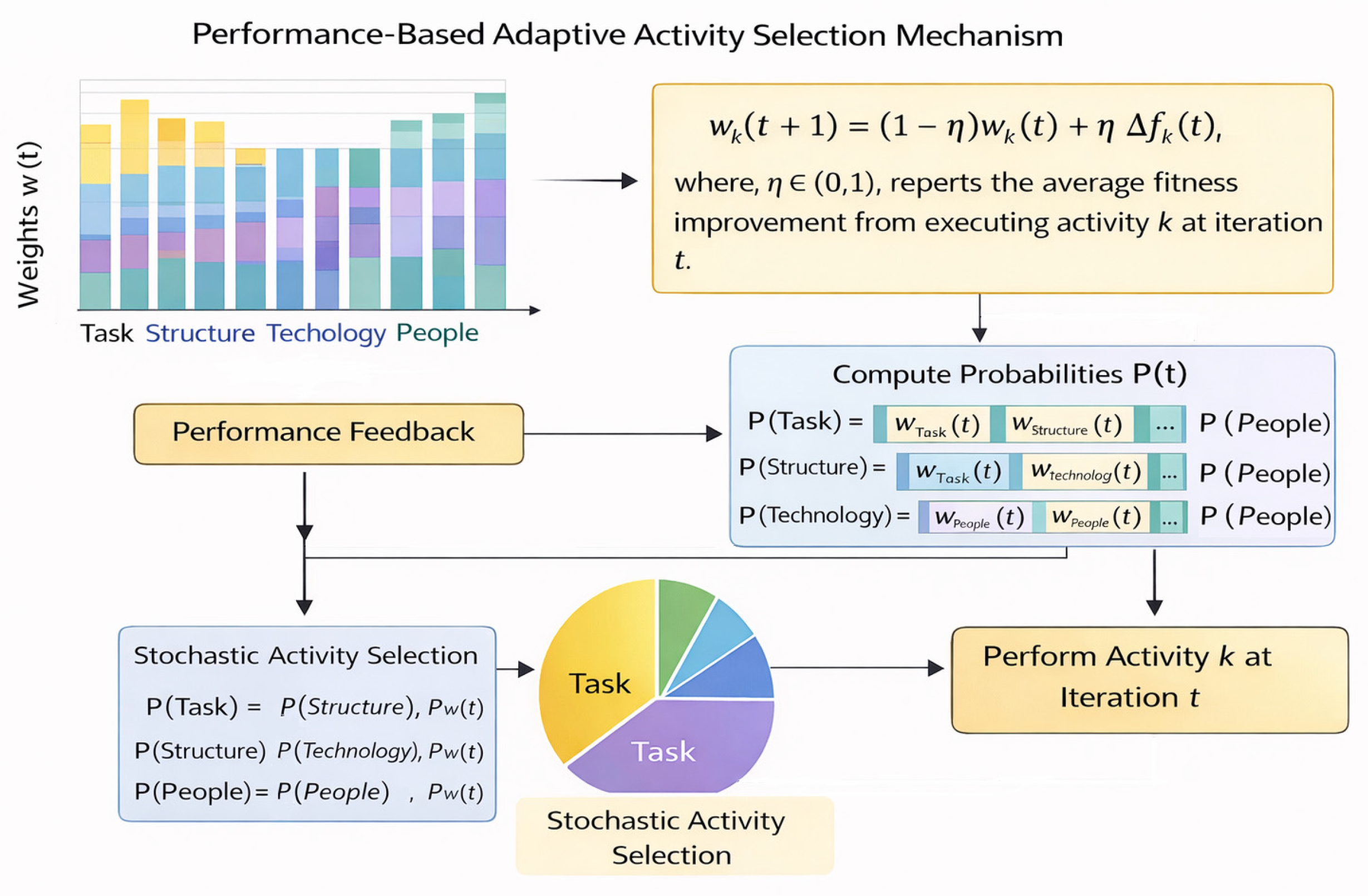
The activity switching mechanism in the original EDOA is primarily determined by a time function $C\left(t\right)$ and a random strategy, lacking the ability to dynamically adapt based on the actual optimization contributions of different activities. However, in real-world business development, organizations often adaptively adjust resource and attention allocation based on the actual impact of different development activities on performance improvement. To address this, this paper proposes an adaptive activity selection mechanism based on performance feedback, enabling the algorithm to dynamically prioritize activity types with greater optimization potential.

A dynamic weight $w_k$ is assigned to each activity to characterize its average performance contribution in historical iterations. The weight update rule is defined as follows:

$$w_k\left(t+1\right)=\left(1-\eta \right)w_k\left(t\right)+\eta \cdot \Delta f_k\left(t\right),$$

(10)

where $\eta \in \left(\mathrm{0,1}\right)$ represents the learning rate, and $\Delta f_k\left(t\right)$ represents the average change in fitness resulting from executing activity $k$ for the $t$-th time. The activity selection probability based on weights can be expressed as

$$P\left(k\right)={\displaystyle \frac{w_k\left(t\right)}{\sum _{j=1}^4 w_j\left(t\right)}}.$$

(11)

In each iteration, the corresponding activity is randomly selected and executed based on the probability distribution described above, thus implementing a performance-driven activity switching strategy. Figure 2 shows a schematic diagram of the strategy.

3.2. Multi-Elite Guided Structural Evolution Strategy

In the original EDOA’s structural update process, the evolution of the organizational structure is primarily guided by the current best solution. This single-elite-driven approach can easily lead to a rapid decrease in population diversity in complex or multimodal optimization problems, thus causing premature convergence. Considering that real-world organizational structure adjustments often draw upon multiple high-performing units, this paper introduces a multi-elite-guided structural evolution mechanism.

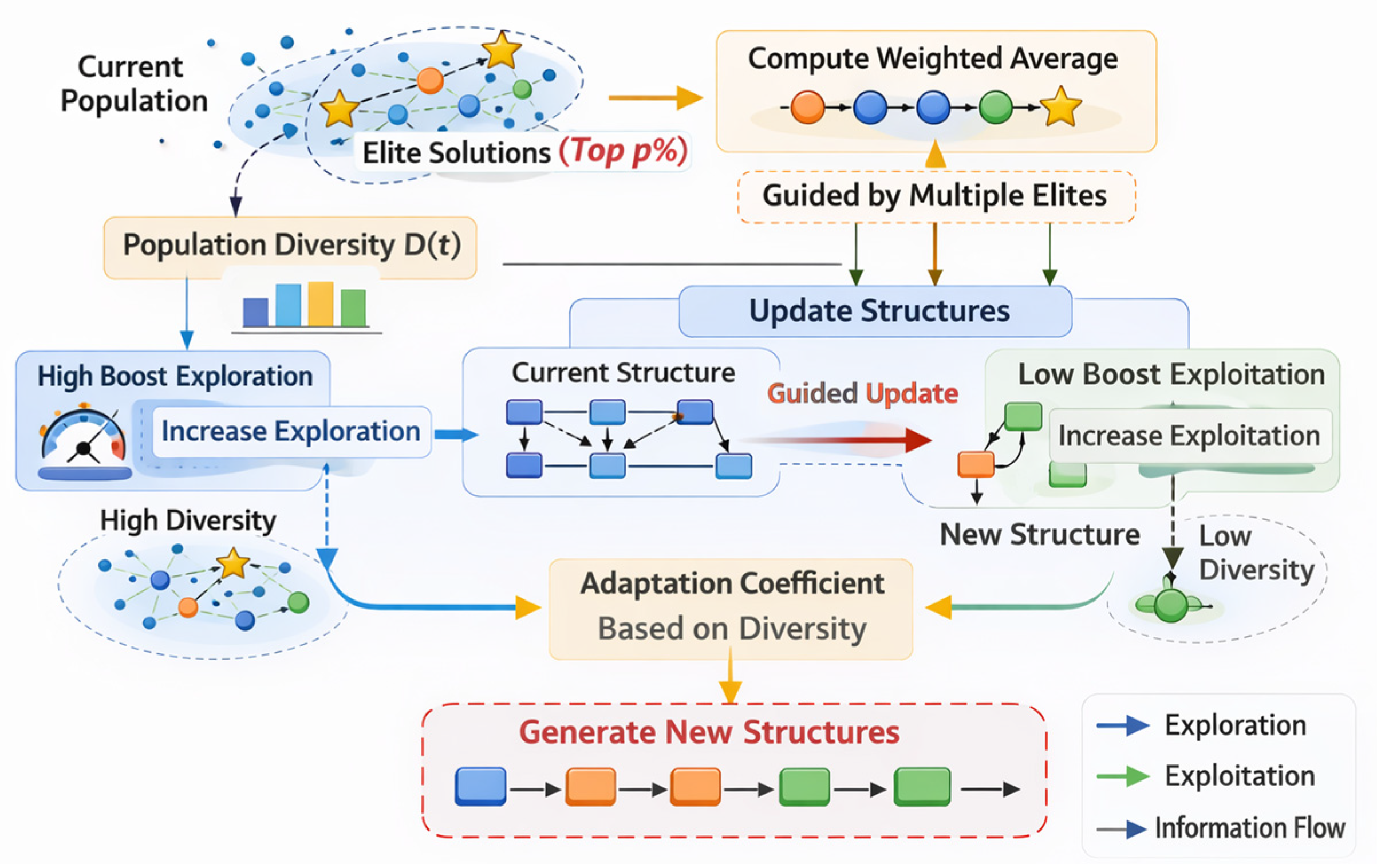
The elite solution set $\mathcal{E}\left(t\right)$ is defined as containing the top $10\mathrm{\%}$ individuals in the current population based on their fitness, and its weighted average is defined as

$$X_{elite}(t)=\sum _{i\in \mathcal{E}\left(t\right)} {\omega }_i{X}_i(t),\sum {\omega }_i=1,$$

(12)

The improved structural update rules are as follows:

$$X_i^s\left(t\right)=X_i^s\left(t-1\right)+\lambda \left(t\right)\cdot rand\left(-\mathrm{1,1}\right)\cdot \left(X_{elite}\left(t-1\right)-X_c^s\left(t-1\right)\right).$$

(13)

In this equation, $X_c^s(t-1)$ represents the centroid of the workflow influenced by the structure, and $\lambda (t)={\displaystyle \frac{1}{N}}\sum _{i=1}^N {∥X_i\left(t\right)-\overline{X}\left(t\right)∥}^2$ is the adaptive coefficient related to population diversity, determined by the population variance, $\overline{X}\left(t\right)$ represents the population center. Figure 3 shows a schematic diagram of this strategy.

3.3. Exploring Technology Lifecycle Awareness—Utilizing Scheduling Mechanisms

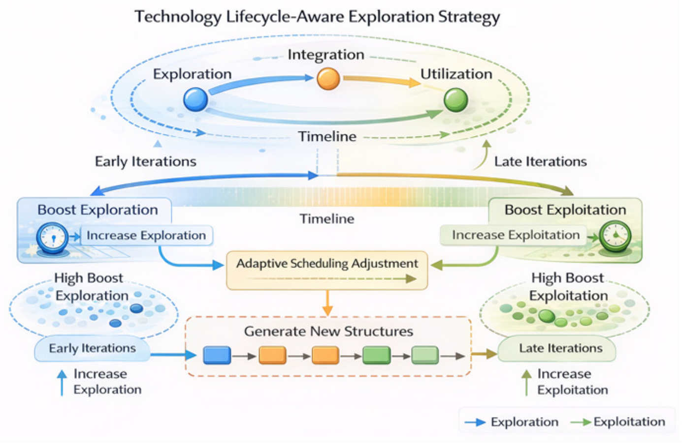
The original EDOA uses fixed random coefficients to control exploration and exploitation behaviors during the technology update phase, which fails to reflect the phased characteristics of “exploration-integration-utilization” in the actual technology evolution process. Therefore, this paper proposes a technology lifecycle-aware exploration-exploitation scheduling strategy to make the technology evolution process more explainable from an organizational behavior perspective.

Define exploration and exploitation control parameters that change with each iteration:

$$\alpha \left(t\right)={\alpha }_0\left(1-{\displaystyle \frac{t}{T}}\right),\beta \left(t\right)={\beta }_0{\displaystyle \frac{t}{T}},$$

(14)

where $T$ represents the maximum number of iterations, and the improved technical update rule is as follows:

$$X_i^t\left(t\right)=X_i^t(t-1)+ran{d}^{\alpha \left(t\right)}\left(\mathrm{0,1}\right)\left(X_{best}(t-1)-X_i^t(t-1)\right)+ran{d}^{\beta \left(t\right)}\left(\mathrm{0,1}\right)\left(X_{rand}(t-1)-X_i^t(t-1)\right)$$

(15)

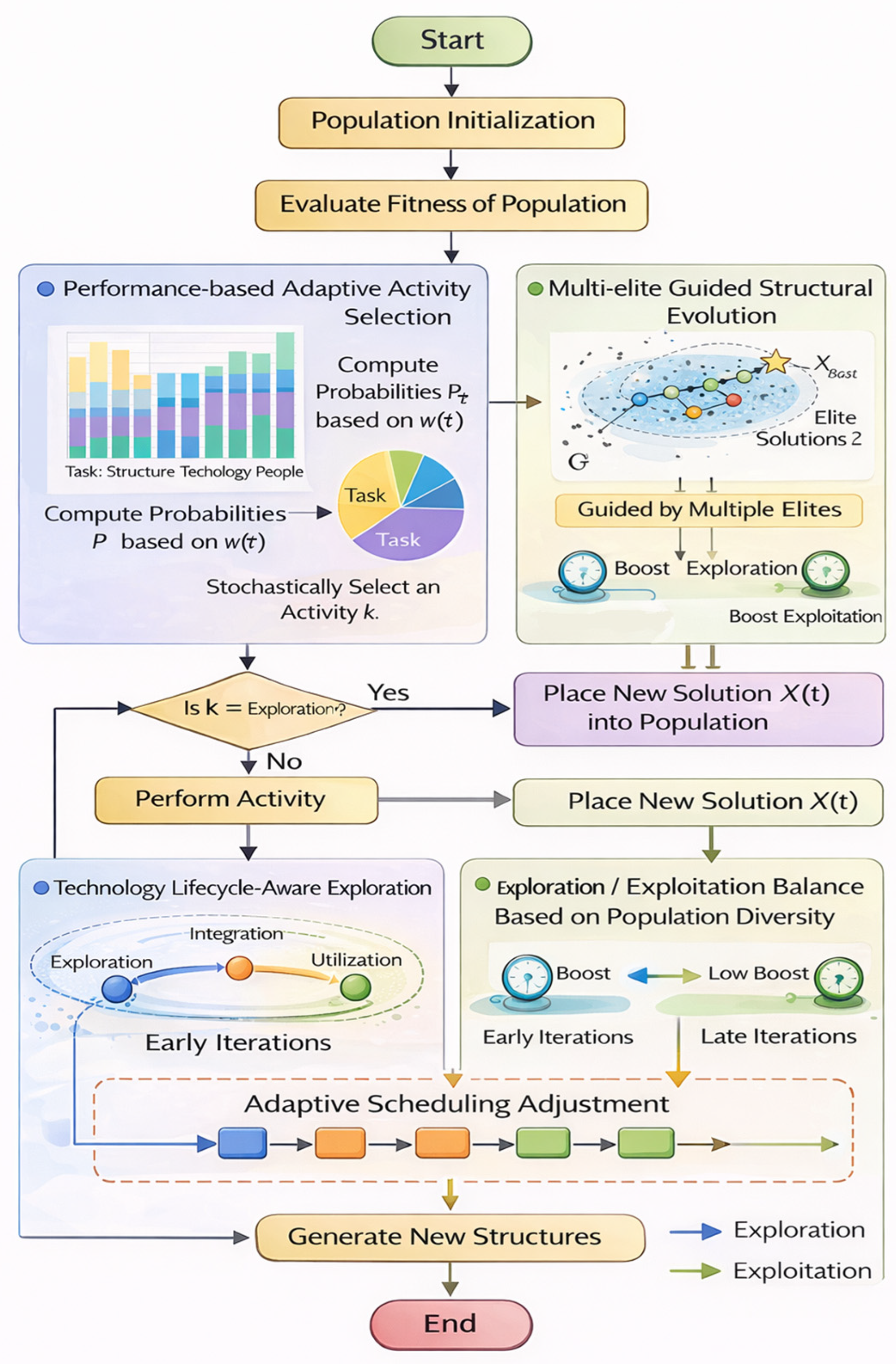
Figure 4 shows a schematic diagram of this strategy. For ease of understanding, the improved algorithm flowchart is shown in Figure 5.

3.4. Computational Complexity Analysis

Let $N$ denote the population size, $D$ the dimensionality of the decision vector, and $T$ the maximum number of iterations. The computational complexity of IEDOA mainly comes from population initialization, fitness evaluation, activity selection, and the position update operations in different evolutionary stages.

During initialization, each individual is generated in a $D$-dimensional search space, resulting in a cost of $O\left(ND\right)$. In each iteration, the algorithm first evaluates the fitness of all individuals, which requires $O(N\cdot C_f)$, where $C_f$ denotes the cost of one objective function evaluation. For general benchmark analysis, if the fitness computation is treated as a constant-cost operation, this part can be simplified as $O\left(N\right)$; however, in practical optimization problems, the fitness evaluation usually dominates the total runtime.

For the activity selection mechanism, the performance-feedback-based adaptive strategy updates the weights and probabilities of four activities only, so its cost is $O\left(1\right)$ per iteration. In the multi-elite-guided structural evolution stage, the algorithm first ranks the population to construct the elite set. A direct sorting operation requires $O\left(N\mathrm{l}\mathrm{o}\mathrm{g}N\right)$, while the weighted averaging of elite individuals and centroid computation both require at most $O\left(ND\right)$. Therefore, the structural evolution stage has a complexity of $O(N\mathrm{l}\mathrm{o}\mathrm{g}N+ND)$. In the lifecycle-aware technology update stage, each individual performs vector operations over $D$ dimensions, leading to a complexity of $O\left(ND\right)$. In the people activity and the task activity inherited from EDOA, the update cost is also bounded by $O\left(ND\right)$ and $O\left(D\right)$, respectively.

Therefore, the overall computational complexity of one iteration of IEDOA can be expressed as $O(N\cdot C_f+N\mathrm{l}\mathrm{o}\mathrm{g}N+ND)$. Since, in most population-based metaheuristic algorithms, $D$ is typically much larger than $\mathrm{l}\mathrm{o}\mathrm{g}N$, the dominant algorithmic overhead is $O\left(ND\right)$ apart from fitness evaluation. Thus, over $T$ iterations, the total computational complexity of IEDOA is $O\left(T\left(N\cdot C_f+ND\right)\right)$. If the fitness evaluation cost is regarded as constant, the total time complexity can be further simplified to $O\left(TND\right)$.

Compared with the original EDOA, the proposed IEDOA introduces three additional mechanisms: adaptive activity feedback, multi-elite guidance, and lifecycle-aware scheduling. Among them, the adaptive feedback and scheduling strategies only introduce negligible constant-level overhead, while the multi-elite mechanism mainly adds a sorting operation and an elite aggregation step. Therefore, IEDOA does not change the overall order of complexity of EDOA and still preserves the computational scalability of population-based metaheuristics. This also agrees with the experimental results under different dimensional settings, where IEDOA maintains good scalability while achieving higher solution quality and stronger robustness.

4. Results of Experiments and Comprehensive Analysis

In this section, IEDOA is assessed using the CEC2017 and CEC2022 benchmark suites. The basic properties of both test sets are first outlined. Next, the parameter configurations and related references of all comparison algorithms are reported to support experimental reproducibility. The performance of IEDOA is then investigated on the CEC2017 benchmark under 30- and 50-dimensional conditions, and on the CEC2022 benchmark with 10- and 20-dimensional settings. Moreover, statistical analyses are performed to verify whether the observed performance differences between IEDOA and other algorithms are statistically significant. For consistency, all algorithms adopt a population size of 50 and a maximum of 1000 iterations. To alleviate the impact of randomness, each algorithm is run 30 independent times, and the average results are used for evaluation. Furthermore, to prevent variations in hardware from affecting algorithm performance, all experiments were conducted under the following conditions: a 12th Gen Intel(R) Core(TM) i9-12900KF (3.20 GHz) processor and MATLAB R2023a. The operating conditions for all algorithms were identical.

4.1. CEC2017 and CEC2022

The CEC2017 [22] and CEC2022 [23] benchmark test suites are widely used in the field of evolutionary computation for evaluating the performance of optimization algorithms. The CEC2017 test set consists of a diverse collection of benchmark functions, including unimodal, multimodal, hybrid, and composition functions, which are designed to assess different optimization capabilities such as convergence speed, global exploration, and local exploitation. The CEC2022 test set is a more recent benchmark suite that further enhances problem complexity by introducing challenging landscapes with higher nonlinearity and variable interactions, thereby reflecting more realistic and difficult optimization scenarios. Owing to their diversity, scalability in dimensionality, and strong representativeness, both CEC2017 and CEC2022 have become standard benchmarks for fair and comprehensive performance evaluation. Therefore, these two test suites are selected in this study to thoroughly validate the effectiveness, robustness, and scalability of the proposed IEDOA across various optimization scenarios.

4.2. Comparison Methods and Parameter Configuration

In this section, we will validate the performance of the proposed IEDOA through comparative experiments with 11 state-of-the-art algorithms, including the Snake optimizer (SO), Gold Rush Optimizer (GRO), Red-tailed Hawk Algorithm (RTH), Genghis Khan Shark Optimizer (GKSO), rime optimization algorithm (RIME), hyper-heuristic whale optimization algorithm (HHWOA), Improved Grey Wolf Optimizer (IGWO), Escape Algorithm (ESC), Runge–Kutta optimizer (RUN), Weighted mean of vectors algorithm (INFO), and the standard Enterprise Development Optimization Algorithm (EDOA). To improve the reproducibility of the experiments, the parameter configurations of all comparative algorithms are summarized in

Table 1. Parameter settings of the comparison algorithms.

Algorithms	Parameter Name	Parameter Value	Reference
SO	$c1$$, c2$$, c3$	0.5, 0.5, 2	[24]
GRO	$sigma$	2	[25]
RTH	$A$$, R_0$$, r$	15, 0.5, 1.5	[26]
GKSO	$h$	0.1	[27]
RIME	$w$	5	[28]
HHWOA	$w$	3	[29]
IGWO	$at$	2	[30]
ESC	$eliteSize$$, a$$, b$	5, 0.15, 0.35	[31]
RUN	$u,v$	20, 12	[32]
INFO	$e$	1 × 10−25	[33]
EDOA	$ishow$	250	[18]

.

4.3. Performance Comparison on the CEC2017 Benchmark

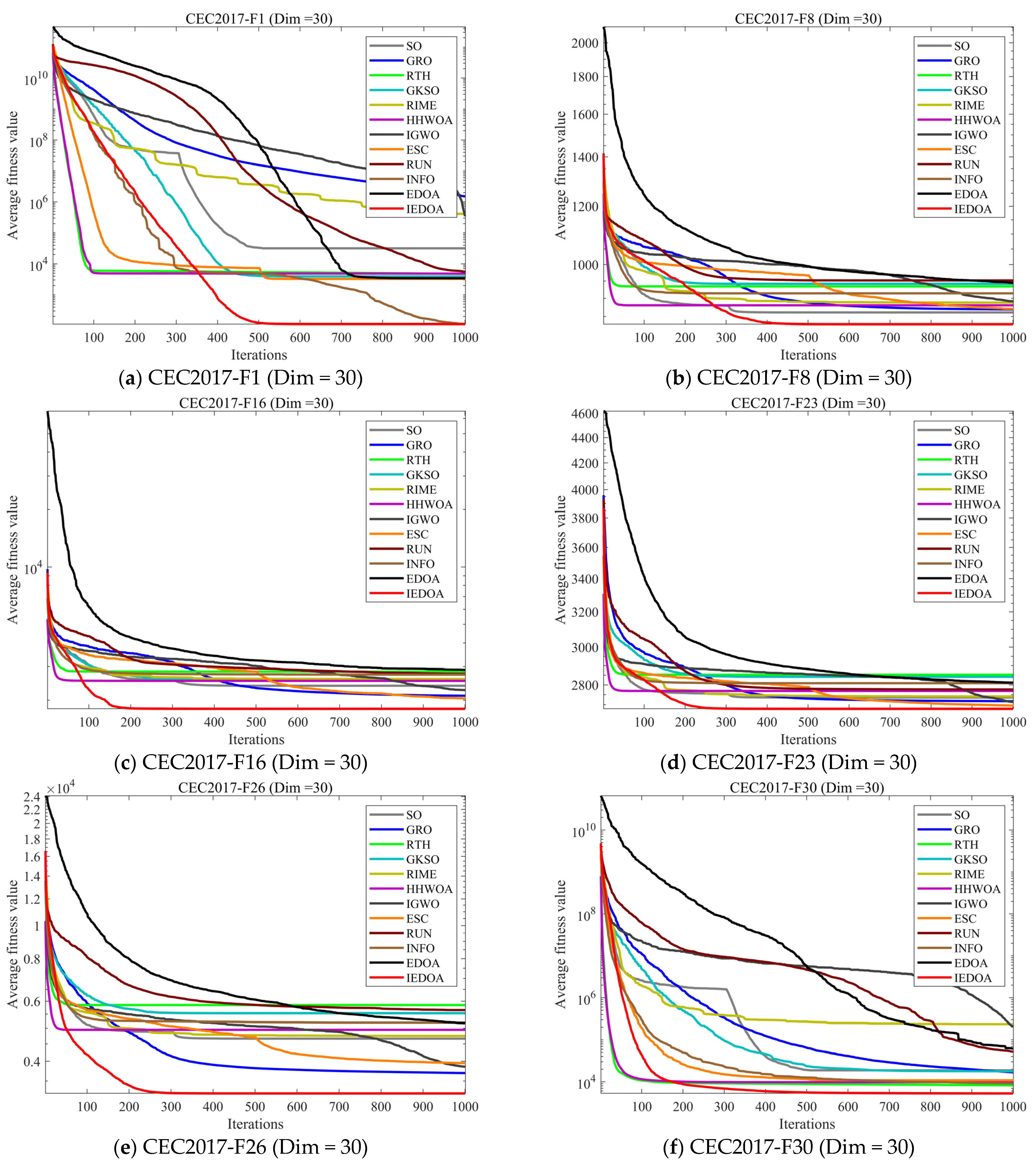
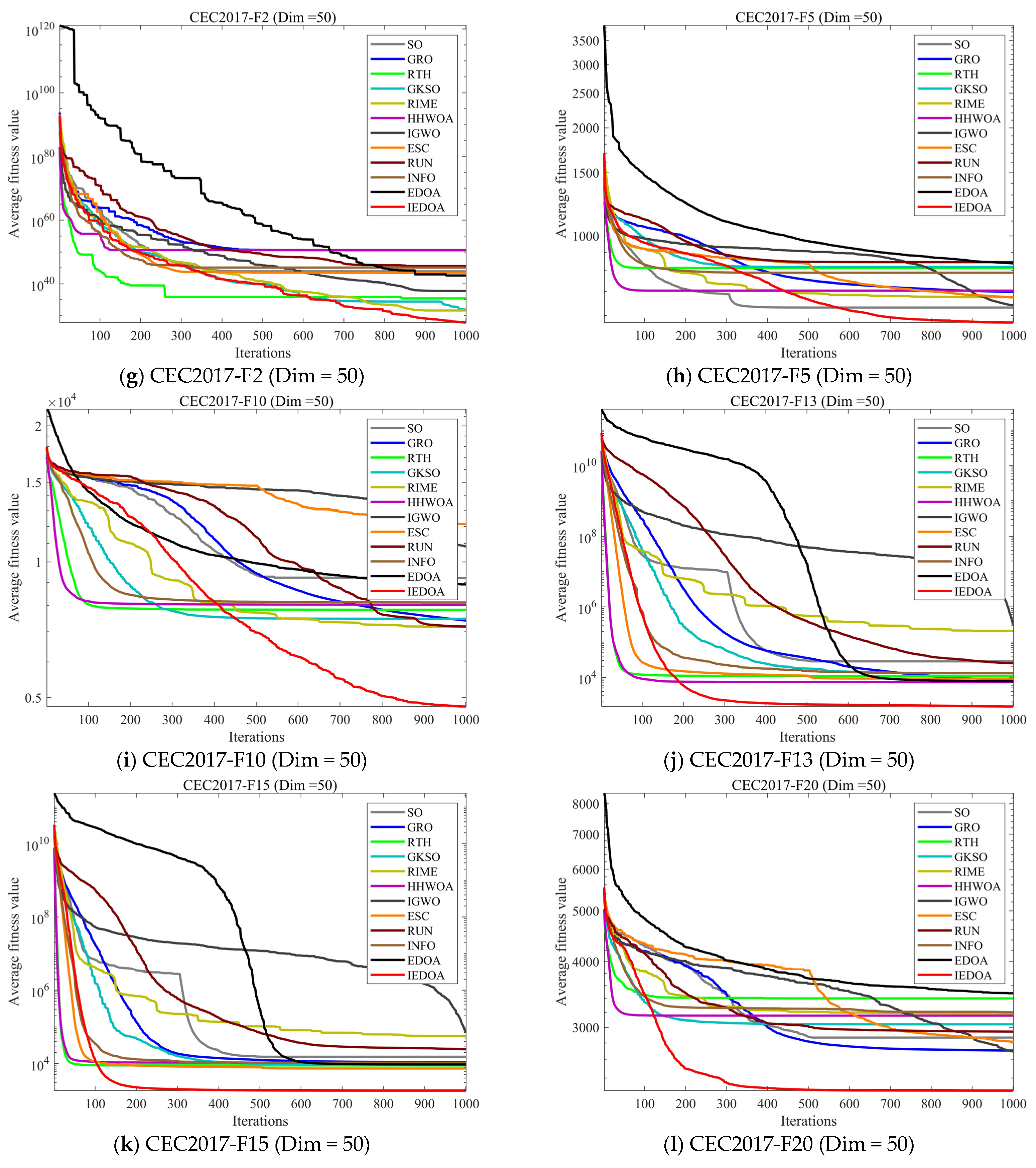
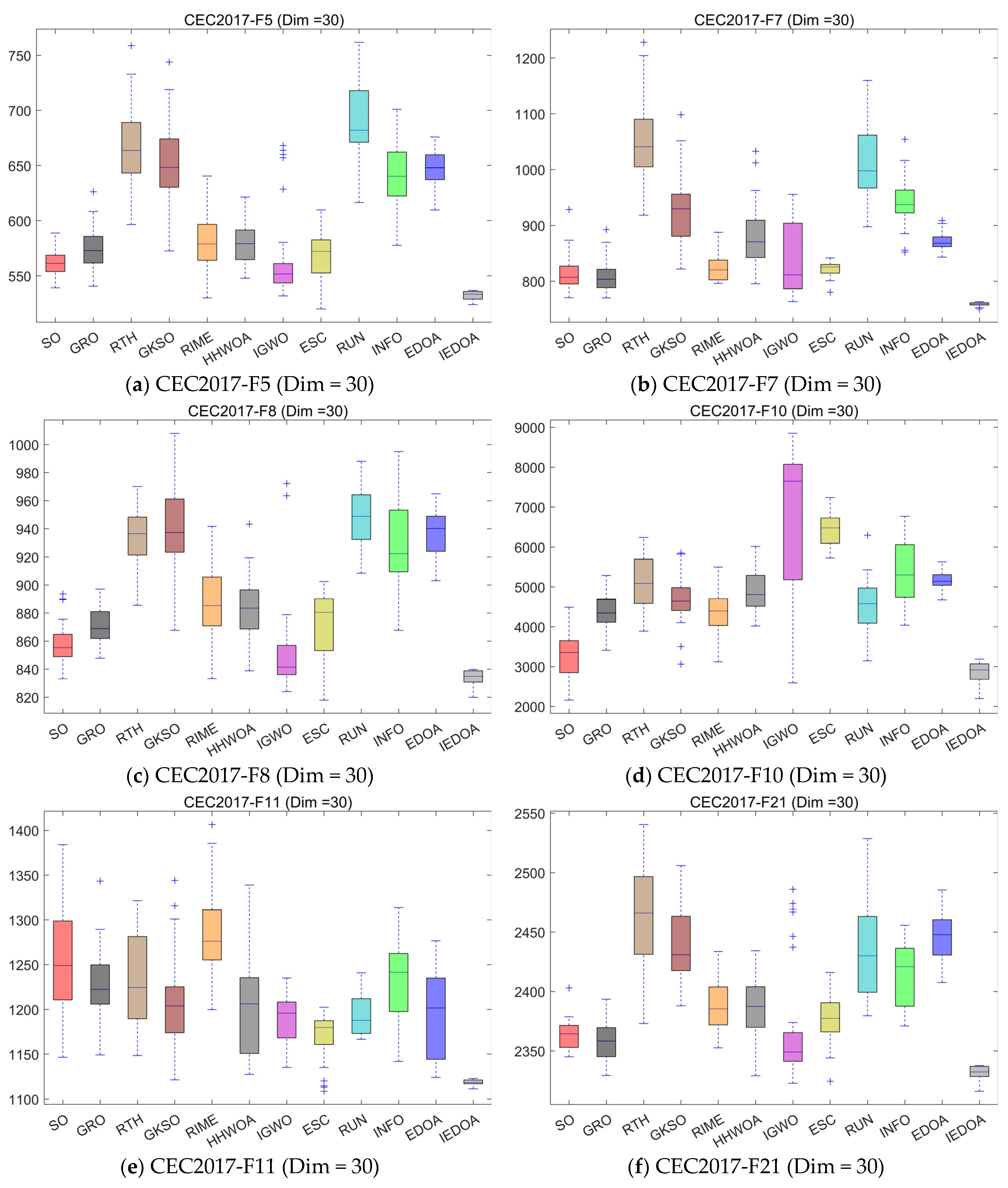
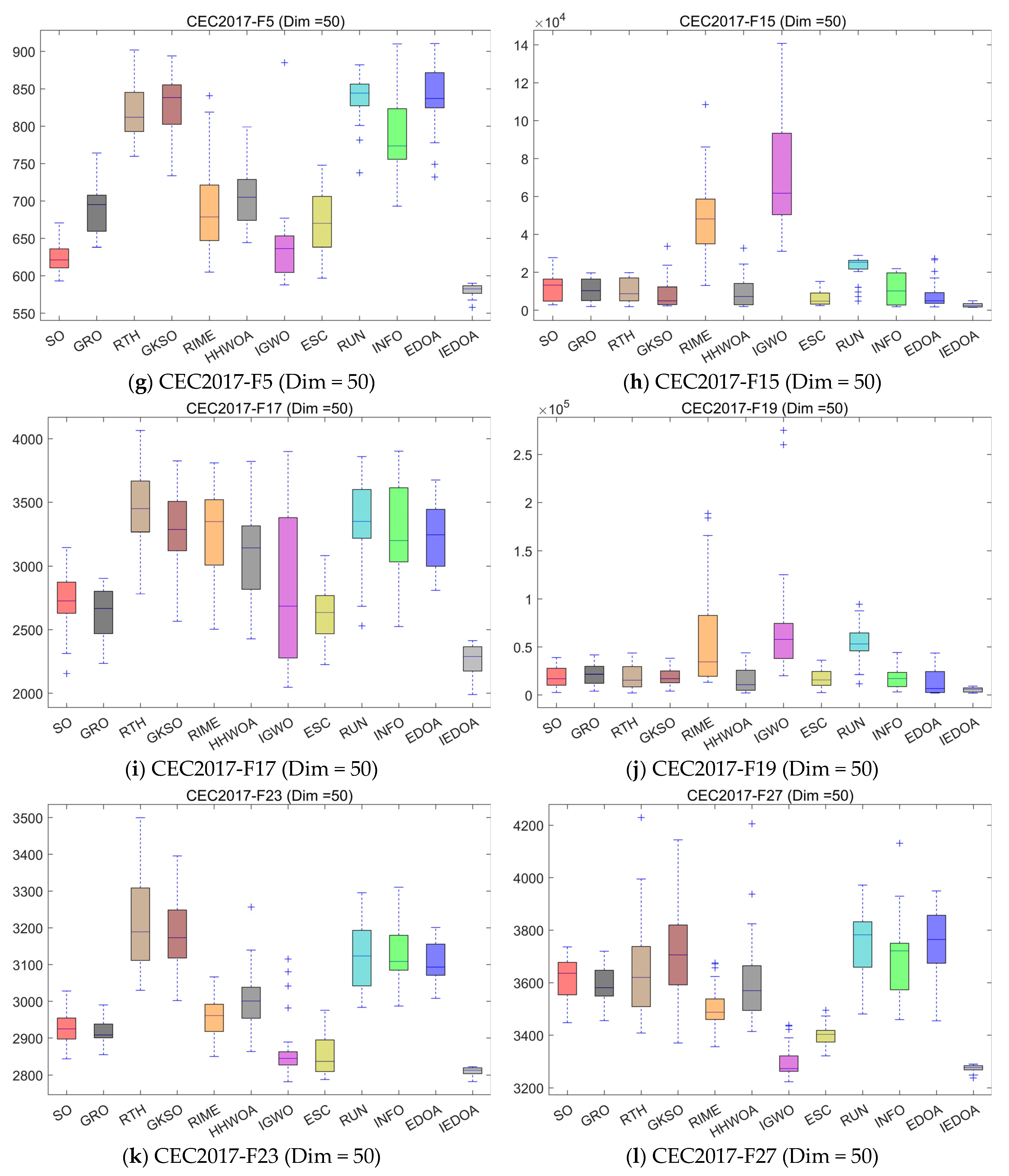
In this section, the performance of IEDOA is investigated on the CEC2017 benchmark test suite. IEDOA is compared with 11 state-of-the-art algorithms under 30-dimensional and 50-dimensional settings. Figure 6 illustrates the convergence behaviors of all compared algorithms across different benchmark functions. The detailed experimental results are summarized in

Table 2. Performance Results on the CEC2017 Benchmark with 30 Dimensions.

ID	Metric	SO	GRO	RTH	GKSO	RIME	HHWOA	IGWO	ESC	RUN	INFO	EDOA	IEDOA
F1	mean	4.3941 × 104	1.2241 × 106	3.0870 × 103	3.4314 × 103	4.5638 × 105	6.0712 × 103	3.4811 × 105	2.6137 × 103	7.5193 × 103	6.1574 × 102	2.5185 × 103	1.6060 × 102
	std	4.5343 × 104	1.4195 × 106	4.3606 × 103	4.8503 × 103	1.9486 × 105	6.0475 × 103	1.8107 × 105	2.6745 × 103	6.6927 × 103	2.4205 × 103	2.7251 × 103	4.9211 × 101
F2	mean	4.8526 × 1017	1.1176 × 1022	1.6735 × 1014	2.0034 × 1012	1.1396 × 1013	6.1641 × 1022	6.3628 × 1016	4.0183 × 1014	4.9287 × 1015	1.5205 × 1017	1.0221 × 1022	1.2677 × 107
	std	1.1803 × 1018	4.8407 × 1022	8.5494 × 1014	4.6803 × 1012	3.3472 × 1013	3.3762 × 1023	1.5027 × 1017	1.5390 × 1015	1.2929 × 1016	5.6850 × 1017	2.3828 × 1022	1.5549 × 107
F3	mean	5.4307 × 104	3.2561 × 104	3.0000 × 102	3.0432 × 102	5.6440 × 103	3.0000 × 102	5.0631 × 103	4.0203 × 104	3.2300 × 102	7.2484 × 102	8.1488 × 104	4.5285 × 104
	std	1.0228 × 104	7.0474 × 103	1.9827 × 10−9	4.3106 × 100	2.3674 × 103	3.2853 × 10−4	3.1495 × 103	1.1708 × 104	3.5471 × 101	7.0908 × 102	1.5933 × 104	6.7738 × 103
F4	mean	4.9714 × 102	5.0937 × 102	4.2193 × 102	4.8910 × 102	5.0987 × 102	4.6690 × 102	4.9500 × 102	5.0300 × 102	5.0342 × 102	4.7317 × 102	4.8440 × 102	4.7300 × 102
	std	2.7243 × 101	1.6621 × 101	2.9264 × 101	3.0384 × 101	2.5785 × 101	3.1422 × 101	1.3078 × 101	1.4670 × 101	1.6894 × 101	2.5159 × 101	3.8354 × 101	1.5186 × 101
F5	mean	5.6105 × 102	5.7482 × 102	6.6645 × 102	6.5203 × 102	5.8080 × 102	5.7898 × 102	5.6701 × 102	5.6880 × 102	6.9063 × 102	6.4288 × 102	6.4796 × 102	5.3245 × 102
	std	1.2759 × 101	1.9689 × 101	3.4852 × 101	3.9716 × 101	2.5562 × 101	1.8345 × 101	4.1975 × 101	2.1785 × 101	3.9229 × 101	3.3991 × 101	1.7224 × 101	4.0474 × 100
F6	mean	6.0282 × 102	6.0389 × 102	6.4277 × 102	6.3495 × 102	6.0404 × 102	6.0619 × 102	6.0039 × 102	6.0000 × 102	6.4621 × 102	6.2047 × 102	6.0333 × 102	6.0000 × 102
	std	2.2000 × 100	1.6895 × 100	9.6897 × 100	8.6561 × 100	1.7202 × 100	4.6388 × 100	1.4212 × 10−1	3.0837 × 10−4	8.4758 × 100	6.4747 × 100	3.8400 × 100	1.3873 × 10−5
F7	mean	8.1558 × 102	8.0893 × 102	1.0527 × 103	9.2567 × 102	8.2426 × 102	8.8343 × 102	8.4025 × 102	8.2199 × 102	1.0070 × 103	9.4336 × 102	8.7086 × 102	7.5895 × 102
	std	3.3087 × 101	2.8746 × 101	7.7361 × 101	6.2580 × 101	2.4141 × 101	5.7634 × 101	6.1123 × 101	1.3056 × 101	6.3625 × 101	4.2978 × 101	1.5681 × 101	3.4977 × 100
F8	mean	8.5790 × 102	8.7007 × 102	9.3449 × 102	9.4201 × 102	8.8693 × 102	8.8401 × 102	8.5227 × 102	8.7269 × 102	9.4831 × 102	9.2951 × 102	9.3702 × 102	8.3379 × 102
	std	1.4881 × 101	1.2600 × 101	2.1634 × 101	3.3104 × 101	2.5600 × 101	2.1860 × 101	3.4109 × 101	2.3780 × 101	2.2793 × 101	2.9774 × 101	1.6462 × 101	5.2525 × 100
F9	mean	1.2013 × 103	1.1486 × 103	4.0825 × 103	3.2579 × 103	1.6647 × 103	1.2810 × 103	9.0964 × 102	9.0045 × 102	3.5013 × 103	2.6482 × 103	1.3169 × 103	9.0025 × 102
	std	1.6803 × 102	1.7325 × 102	8.7554 × 102	9.3675 × 102	8.2217 × 102	3.4606 × 102	1.9687 × 101	5.9083 × 10−1	8.0312 × 102	6.9410 × 102	2.9958 × 102	2.1731 × 10−1
F10	mean	3.2101 × 103	4.3621 × 103	5.0987 × 103	4.6646 × 103	4.3295 × 103	4.8936 × 103	6.7768 × 103	6.4600 × 103	4.5692 × 103	5.3238 × 103	5.1558 × 103	2.8871 × 103
	std	6.2705 × 102	4.4501 × 102	7.3484 × 102	5.8907 × 102	5.2647 × 102	5.2210 × 102	1.8121 × 103	4.4478 × 102	6.8993 × 102	7.9833 × 102	2.2725 × 102	2.4540 × 102
F11	mean	1.2498 × 103	1.2245 × 103	1.2339 × 103	1.2110 × 103	1.2867 × 103	1.2034 × 103	1.1885 × 103	1.1696 × 103	1.1939 × 103	1.2313 × 103	1.1954 × 103	1.1184 × 103
	std	5.6070 × 101	4.0720 × 101	5.2051 × 101	5.3105 × 101	4.8725 × 101	5.6485 × 101	2.6854 × 101	2.6902 × 101	2.2720 × 101	4.3889 × 101	4.8700 × 101	3.3005 × 100
F12	mean	7.2990 × 105	6.7276 × 105	2.4736 × 104	1.3495 × 105	6.1661 × 106	4.1292 × 104	1.7445 × 106	7.1925 × 105	1.0793 × 106	7.8746 × 104	1.9996 × 105	4.4004 × 104
	std	8.3567 × 105	4.2154 × 105	9.8581 × 103	1.3499 × 105	4.0950 × 106	2.8411 × 104	1.6061 × 106	5.3550 × 105	5.8334 × 105	8.9424 × 104	1.5809 × 105	1.8108 × 104
F13	mean	1.6551 × 104	1.6391 × 104	2.2053 × 104	1.3995 × 104	6.2811 × 104	1.4351 × 104	1.3411 × 105	1.2986 × 104	2.7638 × 104	2.1831 × 104	2.5915 × 104	1.6594 × 103
	std	1.1502 × 104	1.2880 × 104	2.1603 × 104	1.4817 × 104	7.5234 × 104	1.7449 × 104	6.9926 × 104	9.4544 × 103	1.4045 × 104	1.9111 × 104	1.9374 × 104	1.9895 × 102
F14	mean	3.5796 × 104	2.0033 × 104	1.7848 × 103	2.1395 × 103	3.9105 × 104	1.4728 × 103	5.3922 × 103	6.9471 × 104	3.2539 × 103	2.2730 × 103	2.7894 × 104	4.1835 × 103
	std	3.8906 × 104	2.1632 × 104	2.0268 × 102	7.7359 × 102	3.5164 × 104	3.8319 × 101	3.6125 × 103	5.7038 × 104	1.7842 × 103	1.6316 × 103	1.7418 × 104	1.4278 × 103
F15	mean	7.9879 × 103	7.2878 × 103	8.2604 × 103	8.2215 × 103	1.7045 × 104	2.5545 × 103	2.2624 × 104	5.5739 × 103	1.4737 × 104	5.5822 × 103	9.7731 × 103	1.6033 × 103
	std	7.7924 × 103	5.8358 × 103	6.8208 × 103	8.0676 × 103	1.3022 × 104	5.3937 × 103	1.8613 × 104	6.0774 × 103	2.2677 × 103	6.0120 × 103	8.7474 × 103	6.1388 × 101
F16	mean	2.3089 × 103	2.1510 × 103	2.7109 × 103	2.4495 × 103	2.6304 × 103	2.6171 × 103	2.1889 × 103	2.0370 × 103	2.7139 × 103	2.6999 × 103	2.8615 × 103	1.9231 × 103
	std	2.0052 × 102	1.9086 × 102	3.1712 × 102	3.2735 × 102	3.1782 × 102	3.4734 × 102	4.3157 × 102	2.3700 × 102	2.5215 × 102	3.2440 × 102	2.3893 × 102	9.7678 × 101
F17	mean	2.0651 × 103	1.8411 × 103	2.4637 × 103	2.1702 × 103	2.0843 × 103	2.1049 × 103	1.8383 × 103	1.8273 × 103	2.1917 × 103	2.2223 × 103	2.1363 × 103	1.7802 × 103
	std	1.4869 × 102	8.0116 × 101	2.5349 × 102	2.5084 × 102	1.9619 × 102	1.8569 × 102	1.0874 × 102	8.4931 × 101	1.8758 × 102	2.8041 × 102	1.1685 × 102	3.1447 × 101
F18	mean	3.2276 × 105	2.4560 × 105	1.7968 × 104	6.5842 × 104	6.0327 × 105	6.3398 × 103	2.2294 × 105	5.3531 × 105	4.8522 × 104	4.2105 × 104	6.0155 × 105	8.0023 × 104
	std	2.3374 × 105	2.4322 × 105	1.9184 × 104	4.3741 × 104	4.6468 × 105	5.3408 × 103	2.1977 × 105	5.5152 × 105	2.3488 × 104	2.3464 × 104	3.1630 × 105	2.4583 × 104
F19	mean	9.4216 × 103	9.0477 × 103	6.5568 × 103	6.7142 × 103	1.1607 × 104	4.4189 × 103	1.4886 × 104	6.0879 × 103	7.6572 × 103	5.2072 × 103	9.7644 × 103	2.1698 × 103
	std	9.8540 × 103	8.1377 × 103	3.9389 × 103	5.0134 × 103	1.0724 × 104	9.7513 × 103	1.5025 × 104	4.8859 × 103	8.5070 × 103	7.3518 × 103	9.4808 × 103	1.9875 × 102
F20	mean	2.3049 × 103	2.2464 × 103	2.7283 × 103	2.4448 × 103	2.4447 × 103	2.4259 × 103	2.1625 × 103	2.1376 × 103	2.4425 × 103	2.5107 × 103	2.5046 × 103	2.0978 × 103
	std	1.3843 × 102	6.8007 × 101	1.7716 × 102	1.5604 × 102	1.8482 × 102	1.8690 × 102	8.4075 × 101	8.7216 × 101	1.3844 × 102	2.0644 × 102	1.3549 × 102	5.4003 × 101
F21	mean	2.3626 × 103	2.3586 × 103	2.4668 × 103	2.4383 × 103	2.3890 × 103	2.3848 × 103	2.3701 × 103	2.3764 × 103	2.4353 × 103	2.4141 × 103	2.4470 × 103	2.3314 × 103
	std	1.2436 × 101	1.6326 × 101	4.3681 × 101	3.2069 × 101	2.3113 × 101	2.5276 × 101	4.9049 × 101	1.9867 × 101	3.8879 × 101	2.7152 × 101	1.7744 × 101	5.5131 × 100
F22	mean	3.8991 × 103	2.3105 × 103	4.1331 × 103	2.7194 × 103	4.3362 × 103	3.4802 × 103	2.7577 × 103	3.8242 × 103	3.2269 × 103	4.2520 × 103	5.7906 × 103	2.3000 × 103
	std	1.7640 × 103	5.9703 × 100	2.1824 × 103	1.2812 × 103	1.8839 × 103	1.7014 × 103	1.7299 × 103	2.3815 × 103	1.6250 × 103	2.1857 × 103	1.6028 × 103	1.2572 × 10−8
F23	mean	2.7461 × 103	2.7072 × 103	2.8457 × 103	2.8565 × 103	2.7474 × 103	2.7798 × 103	2.7078 × 103	2.6985 × 103	2.7926 × 103	2.8024 × 103	2.8103 × 103	2.6832 × 103
	std	1.8440 × 101	2.1208 × 101	6.2393 × 101	6.8101 × 101	2.6260 × 101	3.7126 × 101	4.5940 × 101	1.9245 × 101	3.4942 × 101	3.9358 × 101	1.8275 × 101	4.3108 × 100
F24	mean	2.8925 × 103	2.8723 × 103	3.0557 × 103	3.0246 × 103	2.9214 × 103	2.9269 × 103	2.8926 × 103	2.9080 × 103	2.9242 × 103	2.9978 × 103	2.9747 × 103	2.8523 × 103
	std	1.4132 × 101	1.7443 × 101	6.3557 × 101	7.2220 × 101	2.9068 × 101	4.0848 × 101	5.7249 × 101	2.1599 × 101	2.9695 × 101	7.0319 × 101	2.8584 × 101	4.1660 × 100
F25	mean	2.8939 × 103	2.9118 × 103	2.8921 × 103	2.9057 × 103	2.8968 × 103	2.8951 × 103	2.8871 × 103	2.8889 × 103	2.9033 × 103	2.8985 × 103	2.8907 × 103	2.8838 × 103
	std	9.6389 × 100	1.9767 × 101	1.3400 × 101	2.1587 × 101	1.5415 × 101	1.2835 × 101	1.6394 × 100	3.8475 × 100	1.6467 × 101	2.0399 × 101	9.3552 × 100	1.0023 × 100
F26	mean	4.7596 × 103	3.6706 × 103	5.6058 × 103	5.3025 × 103	4.5543 × 103	4.9514 × 103	4.0397 × 103	3.9315 × 103	4.6593 × 103	5.3325 × 103	5.2899 × 103	3.5922 × 103
	std	4.7161 × 102	7.6167 × 102	1.2072 × 103	1.2376 × 103	6.2198 × 102	4.2808 × 102	1.4974 × 102	1.7396 × 102	1.6533 × 103	9.8329 × 102	2.1751 × 102	4.7962 × 102
F27	mean	3.2614 × 103	3.2358 × 103	3.2568 × 103	3.2656 × 103	3.2319 × 103	3.2532 × 103	3.2000 × 103	3.2142 × 103	3.2652 × 103	3.2491 × 103	3.2372 × 103	3.2023 × 103
	std	1.8553 × 101	1.2404 × 101	3.0513 × 101	3.8172 × 101	1.6557 × 101	2.6483 × 101	1.0585 × 101	1.0605 × 101	2.6704 × 101	2.7425 × 101	1.6962 × 101	5.2113 × 100
F28	mean	3.2659 × 103	3.2610 × 103	3.1407 × 103	3.2136 × 103	3.2527 × 103	3.1597 × 103	3.2192 × 103	3.2205 × 103	3.1994 × 103	3.2052 × 103	3.2241 × 103	3.1722 × 103
	std	2.4523 × 101	3.1088 × 101	5.9975 × 101	2.9083 × 101	2.4102 × 101	6.6882 × 101	1.1382 × 101	1.6213 × 101	2.3183 × 101	2.4266 × 101	2.6676 × 101	3.0584 × 101
F29	mean	3.7978 × 103	3.6239 × 103	4.1652 × 103	4.0152 × 103	3.8885 × 103	3.8755 × 103	3.4888 × 103	3.4611 × 103	4.0654 × 103	4.0266 × 103	3.7785 × 103	3.3913 × 103
	std	1.9295 × 102	1.1619 × 102	2.3320 × 102	2.7189 × 102	2.1999 × 102	2.9134 × 102	9.4692 × 101	9.0337 × 101	2.4902 × 102	2.0959 × 102	1.2476 × 102	4.1957 × 101
F30	mean	2.1714 × 104	1.6928 × 104	7.9354 × 103	1.9585 × 104	1.9918 × 105	8.2108 × 103	2.1932 × 105	1.0032 × 104	5.3893 × 104	9.3753 × 103	2.2032 × 104	5.6296 × 103
	std	3.0730 × 104	1.1876 × 104	2.2497 × 103	1.1983 × 104	1.5625 × 105	2.1029 × 103	1.6406 × 105	3.1533 × 103	2.1747 × 104	3.5476 × 103	1.9388 × 104	2.2232 × 102

and

Table 3. Performance Results on the CEC2017 Benchmark with 50 Dimensions.

ID	Metric	SO	GRO	RTH	GKSO	RIME	HHWOA	IGWO	ESC	RUN	INFO	EDOA	IEDOA
F1	mean	2.5844 × 106	6.4363 × 108	3.0468 × 103	4.1273 × 103	4.4183 × 106	4.3628 × 103	1.4821 × 107	4.2457 × 103	2.0044 × 104	9.0915 × 103	3.6898 × 104	2.9713 × 102
	std	1.6739 × 106	7.1303 × 108	4.0481 × 103	3.4893 × 103	1.5453 × 106	4.6008 × 103	7.9017 × 106	4.3165 × 103	7.0059 × 103	2.0360 × 104	4.2795 × 104	9.8232 × 101
F2	mean	1.2617 × 1044	1.1086 × 1048	2.1537 × 1056	1.6507 × 1032	9.9607 × 1031	1.0493 × 1044	7.2229 × 1040	6.7362 × 1045	1.4887 × 1046	6.1085 × 1044	1.0296 × 1042	6.2911 × 1028
	std	4.9696 × 1044	4.8714 × 1048	1.1797 × 1057	6.0327 × 1032	5.1397 × 1032	5.2351 × 1044	3.9537 × 1041	3.3882 × 1046	8.1286 × 1046	3.3446 × 1045	5.6394 × 1042	8.4478 × 1028
F3	mean	1.3889 × 105	1.0590 × 105	7.6389 × 102	1.1583 × 104	8.2759 × 104	1.2942 × 103	3.5138 × 104	1.5453 × 105	7.9430 × 103	2.5876 × 104	2.2471 × 105	1.6682 × 105
	std	1.6704 × 104	1.3970 × 104	6.0724 × 102	4.2449 × 103	2.1065 × 104	9.3256 × 102	1.1140 × 104	3.0990 × 104	2.9610 × 103	9.2831 × 103	3.3643 × 104	1.4937 × 104
F4	mean	6.0342 × 102	7.0608 × 102	4.8029 × 102	5.8847 × 102	6.1425 × 102	5.2737 × 102	5.9192 × 102	6.0739 × 102	5.5533 × 102	5.4400 × 102	5.5531 × 102	4.7881 × 102
	std	4.3519 × 101	8.3018 × 101	5.6993 × 101	4.3278 × 101	4.2819 × 101	5.3018 × 101	4.9506 × 101	3.8229 × 101	5.8227 × 101	5.0651 × 101	4.6671 × 101	2.5164 × 101
F5	mean	6.2465 × 102	6.8838 × 102	8.1956 × 102	8.2817 × 102	6.9066 × 102	7.0382 × 102	6.3923 × 102	6.6945 × 102	8.3867 × 102	7.8767 × 102	8.3981 × 102	5.8078 × 102
	std	1.9446 × 101	3.3014 × 101	3.5705 × 101	4.2922 × 101	5.9575 × 101	3.4561 × 101	5.3472 × 101	4.3228 × 101	3.0658 × 101	4.9471 × 101	4.2652 × 101	8.0808 × 100
F6	mean	6.0822 × 102	6.1498 × 102	6.4930 × 102	6.5065 × 102	6.1393 × 102	6.1842 × 102	6.0205 × 102	6.0012 × 102	6.5611 × 102	6.3704 × 102	6.2552 × 102	6.0012 × 102
	std	3.0196 × 100	4.7349 × 100	6.7610 × 100	8.1721 × 100	7.2336 × 100	5.8104 × 100	1.0315 × 100	1.1131 × 10−1	5.7638 × 100	7.8595 × 100	5.7607 × 100	2.8941 × 10−2
F7	mean	9.4497 × 102	9.9444 × 102	1.5050 × 103	1.2606 × 103	9.8599 × 102	1.1298 × 103	9.4536 × 102	9.8034 × 102	1.4140 × 103	1.2995 × 103	1.1613 × 103	1.0821 × 103
	std	4.5133 × 101	5.6756 × 101	1.2882 × 102	8.7263 × 101	4.9411 × 101	1.0130 × 102	9.6593 × 101	2.9959 × 101	1.0685 × 102	9.4940 × 101	4.3424 × 101	2.8774 × 101
F8	mean	9.2742 × 102	9.9725 × 102	1.1278 × 103	1.1033 × 103	9.9599 × 102	1.0040 × 103	9.6825 × 102	9.8767 × 102	1.1421 × 103	1.0988 × 103	1.1278 × 103	8.7750 × 102
	std	2.1888 × 101	3.4844 × 101	4.3701 × 101	4.3391 × 101	3.8834 × 101	5.3496 × 101	8.4165 × 101	4.1112 × 101	3.7887 × 101	6.2079 × 101	2.5096 × 101	8.3975 × 100
F9	mean	2.2585 × 103	3.7118 × 103	1.0818 × 104	9.6571 × 103	5.2759 × 103	3.4023 × 103	1.6236 × 103	9.8122 × 102	1.0244 × 104	8.2717 × 103	1.0785 × 104	9.0528 × 102
	std	5.4124 × 102	1.2153 × 103	1.5912 × 103	2.0414 × 103	3.5806 × 103	1.2627 × 103	8.7074 × 102	1.7080 × 102	1.7248 × 103	1.5035 × 103	3.5558 × 103	2.2590 × 100
F10	mean	9.4881 × 103	7.5936 × 103	7.9660 × 103	7.5583 × 103	7.3784 × 103	7.9816 × 103	1.1596 × 104	1.1946 × 104	7.6331 × 103	8.2055 × 103	8.7711 × 103	5.0092 × 103
	std	2.5208 × 103	8.0116 × 102	9.4872 × 102	9.1779 × 102	1.0478 × 103	9.1024 × 102	3.7720 × 103	6.2353 × 102	1.2580 × 103	1.1929 × 103	3.7734 × 102	3.5868 × 102
F11	mean	1.5675 × 103	1.9984 × 103	1.3484 × 103	1.3137 × 103	1.5756 × 103	1.3535 × 103	1.4404 × 103	1.4362 × 103	1.2699 × 103	1.3141 × 103	1.6029 × 103	1.2530 × 103
	std	1.5937 × 102	5.3184 × 102	7.6457 × 101	4.6744 × 101	8.3215 × 101	7.4441 × 101	9.1292 × 101	1.7796 × 102	2.5772 × 101	6.0824 × 101	1.7715 × 102	3.0503 × 101
F12	mean	8.2247 × 106	1.3314 × 107	2.5728 × 105	3.6194 × 106	7.2513 × 107	6.9809 × 105	1.9424 × 107	5.6820 × 106	6.8369 × 106	1.9379 × 106	3.3084 × 106	1.0307 × 106
	std	4.2534 × 106	6.3959 × 106	1.6092 × 105	2.2640 × 106	3.8849 × 107	3.7741 × 105	8.2986 × 106	3.1856 × 106	2.2703 × 106	1.2011 × 106	2.0099 × 106	2.9149 × 105
F13	mean	3.9185 × 104	1.0842 × 104	1.1217 × 104	1.7117 × 104	1.7871 × 105	9.0531 × 103	4.0444 × 105	1.0940 × 104	2.4616 × 104	1.2023 × 104	5.6894 × 103	1.5843 × 103
	std	3.4730 × 104	6.2623 × 103	9.4303 × 103	1.1223 × 104	8.7085 × 104	8.4843 × 103	3.3000 × 105	5.4797 × 103	6.3118 × 103	8.8395 × 103	4.1373 × 103	1.0190 × 102
F14	mean	2.1186 × 105	1.3744 × 105	5.7897 × 103	2.7497 × 104	2.4117 × 105	9.0785 × 103	8.1063 × 104	2.7302 × 105	2.2729 × 104	2.9895 × 104	5.8247 × 105	1.9975 × 104
	std	1.4486 × 105	1.4741 × 105	2.6781 × 103	2.7983 × 104	1.2210 × 105	9.1697 × 103	5.4514 × 104	3.1802 × 105	1.5630 × 104	3.5040 × 104	5.0879 × 105	7.2772 × 103
F15	mean	1.2512 × 104	1.0428 × 104	1.0150 × 104	8.5574 × 103	5.0281 × 104	9.4876 × 103	6.9727 × 104	6.2466 × 103	2.2858 × 104	1.1042 × 104	8.0562 × 103	2.7342 × 103
	std	7.2463 × 103	5.7821 × 103	6.2504 × 103	7.4612 × 103	1.9565 × 104	7.7101 × 103	2.7927 × 104	3.6280 × 103	6.2632 × 103	7.5028 × 103	7.0644 × 103	1.1398 × 103
F16	mean	2.9605 × 103	2.7235 × 103	3.6838 × 103	3.3782 × 103	3.4789 × 103	3.3364 × 103	2.5273 × 103	3.0330 × 103	3.3060 × 103	3.4511 × 103	4.0678 × 103	2.4941 × 103
	std	3.4891 × 102	2.9190 × 102	5.0910 × 102	4.5727 × 102	5.7281 × 102	4.1656 × 102	4.4313 × 102	4.0319 × 102	4.0021 × 102	4.2715 × 102	2.8920 × 102	1.8818 × 102
F17	mean	2.7214 × 103	2.6380 × 103	3.4219 × 103	3.3120 × 103	3.2560 × 103	3.1083 × 103	2.8032 × 103	2.6297 × 103	3.3230 × 103	3.2323 × 103	3.2427 × 103	2.2625 × 103
	std	2.1269 × 102	1.9688 × 102	3.0739 × 102	2.9246 × 102	3.6107 × 102	3.3951 × 102	5.7811 × 102	2.1297 × 102	3.6689 × 102	3.7151 × 102	2.5951 × 102	1.1364 × 102
F18	mean	1.9211 × 106	2.1707 × 106	2.9237 × 104	1.9073 × 105	3.4739 × 106	3.7354 × 104	8.0992 × 105	2.1771 × 106	7.3332 × 104	1.6590 × 105	3.3920 × 106	2.9549 × 105
	std	1.4957 × 106	1.5028 × 106	1.4980 × 104	1.0629 × 105	2.3063 × 106	3.2414 × 104	5.2803 × 105	1.7295 × 106	2.6982 × 104	1.9718 × 105	1.3698 × 106	9.2352 × 104
F19	mean	1.8785 × 104	2.1824 × 104	1.8717 × 104	1.8300 × 104	5.5974 × 104	1.6737 × 104	7.0839 × 104	1.7654 × 104	5.2718 × 104	1.7465 × 104	1.2501 × 104	5.5408 × 103
	std	1.1287 × 104	1.0783 × 104	1.3436 × 104	9.1263 × 103	5.1182 × 104	1.3843 × 104	5.8858 × 104	9.1519 × 103	1.8325 × 104	1.0583 × 104	1.2795 × 104	2.3633 × 103
F20	mean	3.1403 × 103	2.6776 × 103	3.3326 × 103	3.1458 × 103	3.1524 × 103	3.1022 × 103	2.7537 × 103	2.7389 × 103	3.1160 × 103	3.3025 × 103	3.4391 × 103	2.3342 × 103
	std	4.4668 × 102	2.1681 × 102	3.0641 × 102	3.4799 × 102	3.1653 × 102	3.0897 × 102	4.8595 × 102	2.2215 × 102	2.6575 × 102	3.2463 × 102	1.9424 × 102	1.0141 × 102
F21	mean	2.4305 × 103	2.4603 × 103	2.6412 × 103	2.6303 × 103	2.4802 × 103	2.4889 × 103	2.4322 × 103	2.4879 × 103	2.6040 × 103	2.5928 × 103	2.6438 × 103	2.3774 × 103
	std	2.4263 × 101	2.9671 × 101	6.4106 × 101	6.6666 × 101	4.5989 × 101	3.3999 × 101	5.6809 × 101	3.6145 × 101	4.8502 × 101	6.6124 × 101	3.6161 × 101	1.1106 × 101
F22	mean	1.0999 × 104	6.5191 × 103	9.8149 × 103	9.8039 × 103	9.3652 × 103	9.4671 × 103	1.2211 × 104	1.3474 × 104	9.4141 × 103	9.8987 × 103	1.1118 × 104	4.2878 × 103
	std	2.7817 × 103	3.1647 × 103	1.0822 × 103	1.0654 × 103	1.1006 × 103	1.0021 × 103	4.1107 × 103	7.0046 × 102	1.7516 × 103	1.2248 × 103	4.8108 × 102	2.0423 × 103
F23	mean	2.9278 × 103	2.9152 × 103	3.2183 × 103	3.1810 × 103	2.9576 × 103	3.0039 × 103	2.8684 × 103	2.8546 × 103	3.1241 × 103	3.1280 × 103	3.1073 × 103	2.8099 × 103
	std	4.1129 × 101	3.0236 × 101	1.2644 × 102	9.7531 × 101	5.2145 × 101	8.3520 × 101	7.9760 × 101	5.1536 × 101	8.1904 × 101	8.2761 × 101	4.9891 × 101	1.1848 × 101
F24	mean	3.0626 × 103	3.0704 × 103	3.3918 × 103	3.3730 × 103	3.1042 × 103	3.1586 × 103	3.0305 × 103	3.1273 × 103	3.1484 × 103	3.2504 × 103	3.3154 × 103	2.9774 × 103
	std	3.4327 × 101	3.3563 × 101	1.3673 × 102	9.8084 × 101	4.2347 × 101	7.0177 × 101	7.9575 × 101	3.3322 × 101	5.8417 × 101	8.7529 × 101	6.1607 × 101	9.1692 × 100
F25	mean	3.1018 × 103	3.2707 × 103	3.0435 × 103	3.0872 × 103	3.1047 × 103	3.0495 × 103	3.0931 × 103	3.0943 × 103	3.0930 × 103	3.0835 × 103	3.0863 × 103	3.0105 × 103
	std	3.9965 × 101	7.0148 × 101	4.1629 × 101	2.5016 × 101	4.0491 × 101	4.4931 × 101	4.1934 × 101	3.1058 × 101	2.8763 × 101	2.7813 × 101	3.2323 × 101	1.6772 × 101
F26	mean	5.9778 × 103	5.6938 × 103	8.6510 × 103	7.2657 × 103	6.0667 × 103	7.2435 × 103	5.2948 × 103	4.7975 × 103	1.1212 × 104	8.6644 × 103	7.2832 × 103	3.9497 × 103
	std	4.0543 × 102	1.4887 × 103	2.5814 × 103	3.6367 × 103	4.9000 × 102	7.7381 × 102	7.3992 × 102	3.8897 × 102	1.5051 × 103	2.1280 × 103	3.7962 × 102	8.1403 × 102
F27	mean	3.6129 × 103	3.5870 × 103	3.6572 × 103	3.7135 × 103	3.5069 × 103	3.6072 × 103	3.2983 × 103	3.3979 × 103	3.7491 × 103	3.6880 × 103	3.7555 × 103	3.2749 × 103
	std	8.5905 × 101	6.9321 × 101	1.7886 × 102	1.6804 × 102	8.0532 × 101	1.6898 × 102	5.7230 × 101	4.0430 × 101	1.3654 × 102	1.4400 × 102	1.3233 × 102	1.3105 × 101
F28	mean	3.4431 × 103	3.6389 × 103	3.2921 × 103	3.3231 × 103	3.3593 × 103	3.3055 × 103	3.3626 × 103	3.4677 × 103	3.3290 × 103	3.3330 × 103	3.3703 × 103	3.2615 × 103
	std	5.8318 × 101	8.2448 × 101	2.9215 × 101	3.0966 × 101	3.5293 × 101	2.1612 × 101	4.0538 × 101	8.8826 × 101	2.5978 × 101	2.7532 × 101	4.1470 × 101	1.3970 × 100
F29	mean	4.4708 × 103	4.1713 × 103	4.7488 × 103	5.1949 × 103	4.6825 × 103	4.7074 × 103	3.8262 × 103	3.5985 × 103	5.1680 × 103	4.8414 × 103	4.6719 × 103	3.4972 × 103
	std	2.9530 × 102	2.1885 × 102	4.3163 × 102	4.0937 × 102	3.1136 × 102	3.8766 × 102	2.4237 × 102	2.0554 × 102	4.9083 × 102	2.7176 × 102	3.8269 × 102	1.0081 × 102
F30	mean	2.6407 × 106	1.5840 × 106	8.5922 × 105	5.6070 × 106	2.5479 × 107	1.1419 × 106	7.3193 × 106	1.2935 × 106	7.5518 × 106	8.3846 × 105	2.9623 × 106	7.3677 × 105
	std	1.2076 × 106	3.6629 × 105	1.5107 × 105	2.0879 × 106	8.5677 × 106	5.0828 × 105	2.8163 × 106	3.1262 × 105	1.6553 × 106	1.3866 × 105	1.0458 × 106	4.2144 × 104

, where “mean” and “std” denote the average value and standard deviation obtained from 30 independent runs, respectively. Furthermore, to provide a more comprehensive comparison, the distribution of results over 30 runs is visualized using box plots in Figure 7.

As shown in Figure 6, the convergence curves of the different algorithms on the CEC2017 test set exhibit significant differences: compared to the original EDOA and other comparison algorithms, IEDOA is able to reduce the objective function value at a faster rate on most functions and maintains a more stable downward trend in the later stages of iteration, ultimately achieving higher convergence accuracy. This indicates that IEDOA’s improved strategy helps enhance global exploration capabilities and accelerate the approach to high-quality solutions in the early stages of the search, while effectively maintaining exploitation capabilities in the later stages, reducing oscillations and avoiding getting trapped in local optima. Therefore, it demonstrates stronger overall advantages in both convergence speed and the quality of the final solution.

As shown in the box plot results in Figure 7, IEDOA demonstrates superior and more stable optimization performance on the CEC2017 test set for most benchmark functions: its box is generally lower, indicating smaller objective function values and higher solution quality; at the same time, the box height and the length of the whiskers are generally shorter, indicating less fluctuation in the results of multiple independent runs and stronger robustness. In contrast, some of the comparison algorithms have higher boxes and greater dispersion, and even show many outliers, reflecting their unstable convergence results or susceptibility to randomness. Overall, the box plot confirms that IEDOA has significant advantages in both solution accuracy and stability, enabling it to reliably obtain high-quality solutions in complex multimodal and mixed-characteristic problems.

The experimental results from Table 2 (30 dimensions) and Table 3 (50 dimensions) show that IEDOA performs best overall in the CEC2017 benchmark tests: under both dimensional settings, IEDOA achieved smaller optimal/average objective function values on most test functions and demonstrated stronger overall problem-solving capabilities compared to other algorithms. As the dimensionality increased from 30 to 50, the performance of all algorithms generally decreased to varying degrees, indicating that the high-dimensional search space significantly increased the optimization difficulty; however, IEDOA still maintained good solution quality and a competitive advantage, demonstrating its stronger adaptability and stability to dimensional expansion. Overall, the consistent advantage across both dimensions verifies that the improved strategy of IEDOA effectively balances exploration and exploitation in complex high-dimensional problems, thus outperforming the original EDOA and other mainstream algorithms in both accuracy and robustness.

4.4. Performance Comparison on the CEC2022 Benchmark

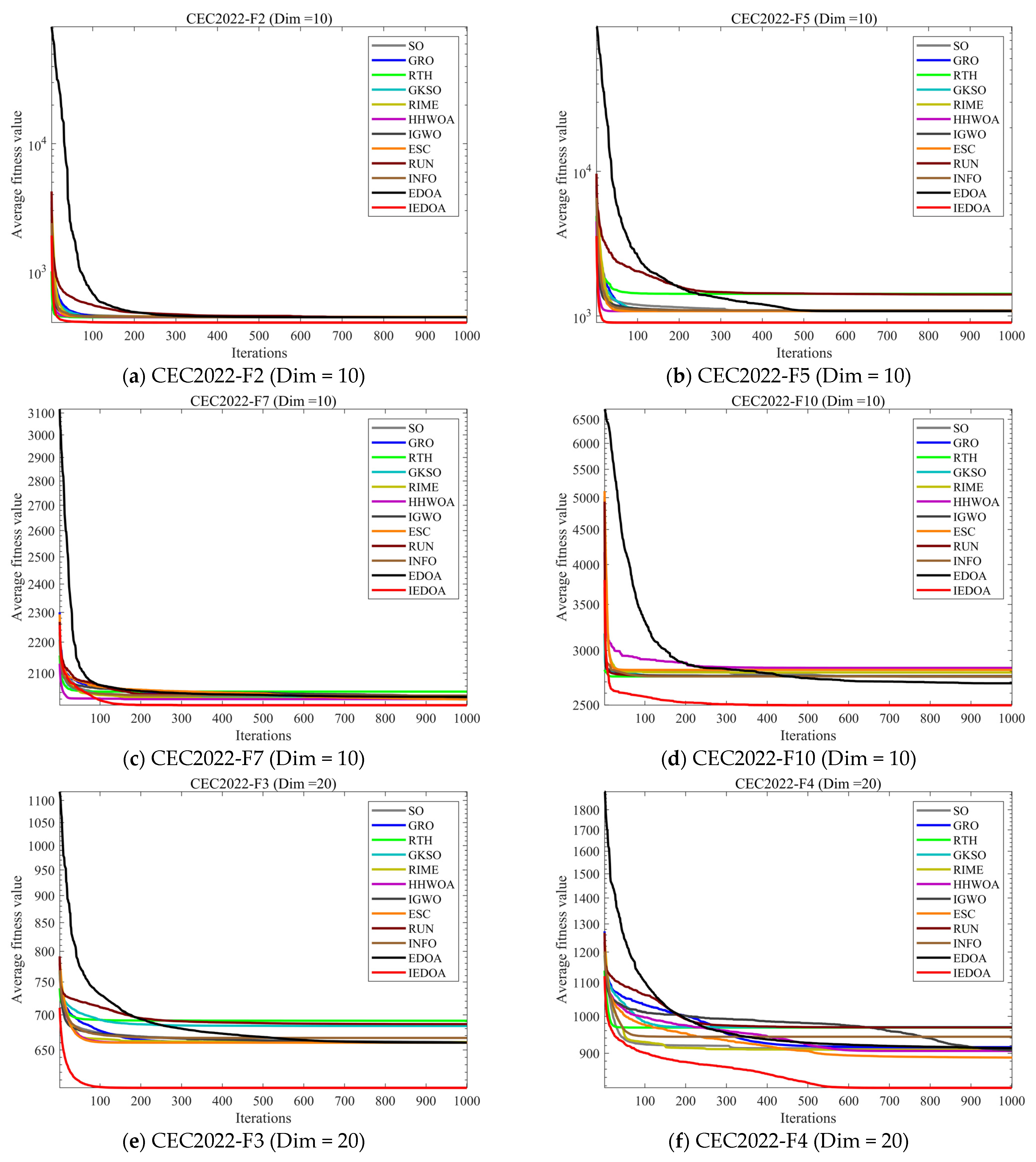
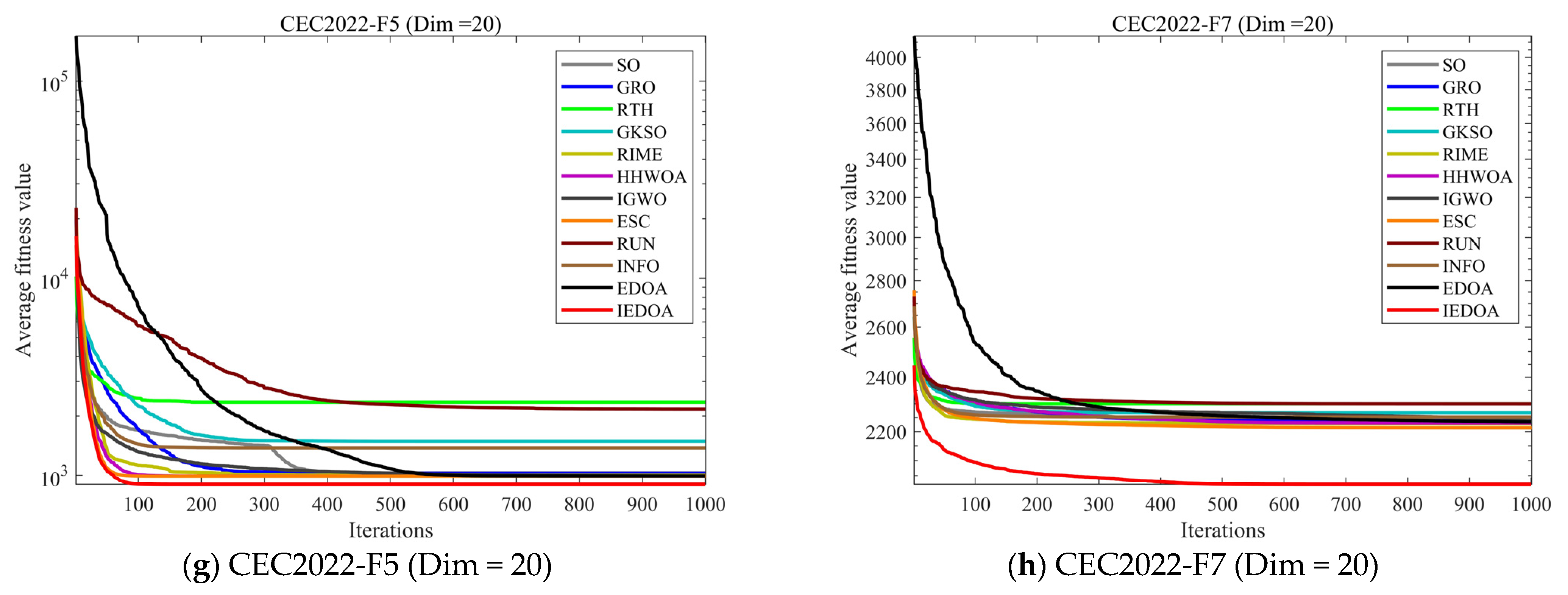
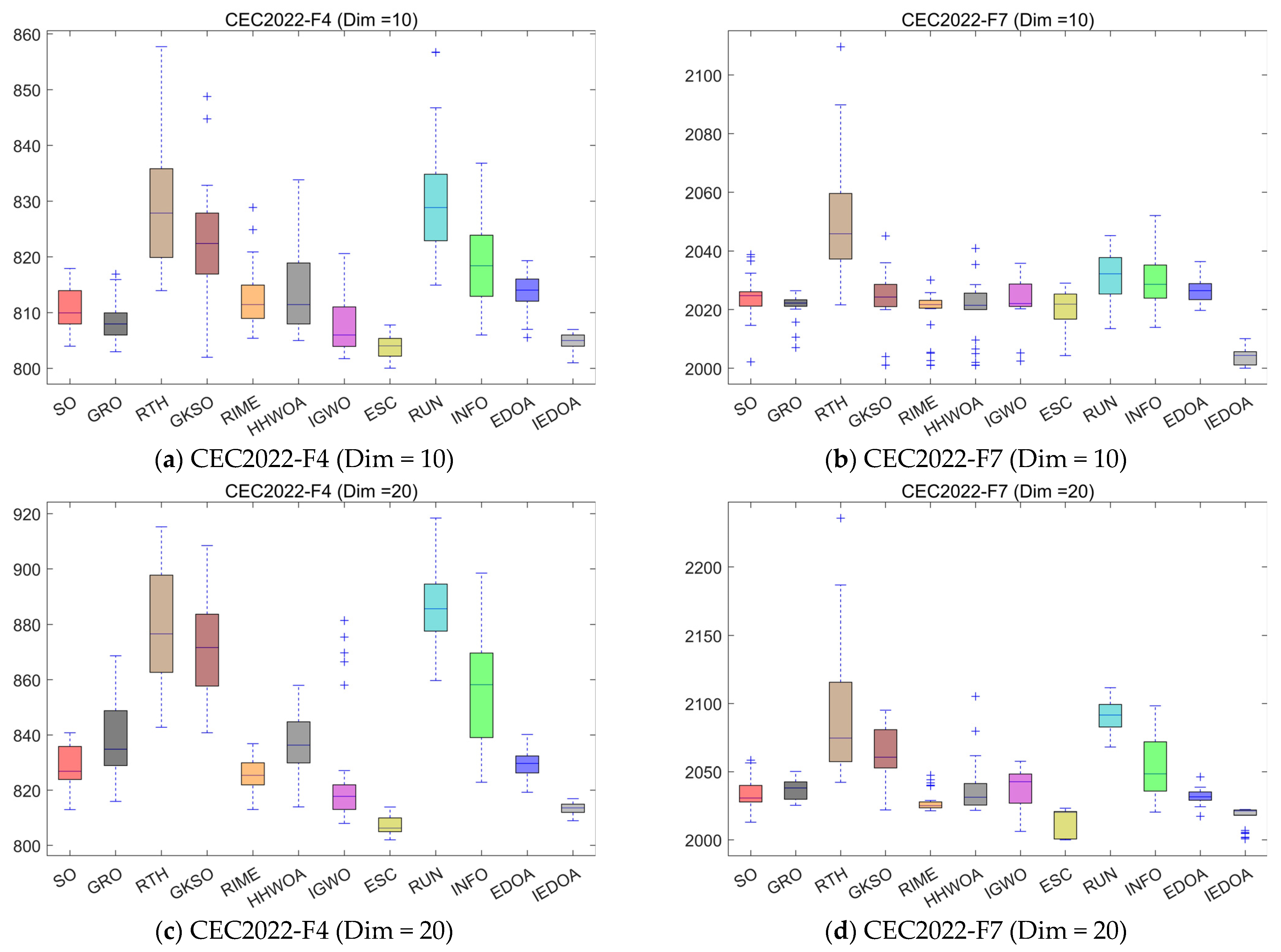
In this section, the performance of IEDOA is evaluated using the CEC2022 benchmark suite. A comparative study is conducted between IEDOA and 11 advanced algorithms under 10- and 20-dimensional settings. Figure 8 presents the convergence curves of all algorithms across the benchmark functions. Detailed numerical results are listed in

Table 4. Performance Results on the CEC2022 Benchmark with 10 Dimensions.

ID	Metric	SO	GRO	RTH	GKSO	RIME	HHWOA	IGWO	ESC	RUN	INFO	EDOA	IEDOA
F1	mean	3.0025 × 102	3.2588 × 102	3.0000 × 102	3.0000 × 102	3.0008 × 102	3.0000 × 102	3.0009 × 102	3.0339 × 102	3.0000 × 102	3.0000 × 102	5.0392 × 102	3.0000 × 102
	std	5.2511 × 10−1	7.0226 × 101	4.7206 × 10−14	3.1326 × 10−12	6.5481 × 10−2	2.3198 × 10−13	8.2205 × 10−2	5.6752 × 100	4.5688 × 10−5	1.0449 × 10−13	1.7505 × 102	0.0000 × 100
F2	mean	4.0164 × 102	4.0300 × 102	4.0000 × 102	4.0000 × 102	4.0548 × 102	4.0017 × 102	4.0084 × 102	4.0359 × 102	4.0003 × 102	4.0000 × 102	4.0015 × 102	4.0016 × 102
	std	1.6365 × 100	1.8966 × 100	1.7899 × 10−12	1.5161 × 10−2	1.3427 × 101	7.8123 × 10−2	5.7720 × 10−1	7.1200 × 10−1	2.1332 × 10−2	6.2149 × 10−5	3.0772 × 10−1	1.1191 × 10−1
F3	mean	6.0001 × 102	6.0000 × 102	6.0880 × 102	6.0176 × 102	6.0006 × 102	6.0003 × 102	6.0003 × 102	6.0000 × 102	6.0809 × 102	6.0035 × 102	6.0000 × 102	6.0000 × 102
	std	1.8690 × 10−2	6.4328 × 10−3	7.7105 × 100	2.3943 × 100	2.7184 × 10−2	7.2147 × 10−2	7.7821 × 10−3	2.7941 × 10−5	3.9232 × 100	8.9571 × 10−1	1.2190 × 10−4	0.0000 × 100
F4	mean	8.1048 × 102	8.0849 × 102	8.2894 × 102	8.2292 × 102	8.1253 × 102	8.1406 × 102	8.0787 × 102	8.0371 × 102	8.2930 × 102	8.1912 × 102	8.1366 × 102	8.0491 × 102
	std	3.8289 × 100	3.2607 × 100	1.0373 × 101	9.9340 × 100	5.3767 × 100	7.5954 × 100	5.3721 × 100	1.8748 × 100	9.5989 × 100	7.6985 × 100	3.3726 × 100	1.1955 × 100
F5	mean	9.0031 × 102	9.0002 × 102	1.1133 × 103	9.0186 × 102	9.0007 × 102	9.0245 × 102	9.0001 × 102	9.0000 × 102	1.1261 × 103	9.2027 × 102	9.0008 × 102	9.0000 × 102
	std	1.0115 × 100	8.4910 × 10−2	3.4853 × 102	2.3405 × 100	1.3264 × 10−1	4.3166 × 100	3.9888 × 10−3	3.7766 × 10−7	1.3862 × 102	4.3495 × 101	1.4512 × 10−1	0.0000 × 100
F6	mean	3.6408 × 103	2.9464 × 103	1.8599 × 103	3.2397 × 103	7.3559 × 103	1.8025 × 103	3.9197 × 103	3.9029 × 103	3.3177 × 103	1.8494 × 103	2.4258 × 103	1.9118 × 103
	std	2.4409 × 103	1.4072 × 103	4.4432 × 101	2.8593 × 103	5.3945 × 103	7.5196 × 100	2.2372 × 103	2.4811 × 103	1.7080 × 103	3.9283 × 101	3.8460 × 102	6.4719 × 101
F7	mean	2.0246 × 103	2.0215 × 103	2.0492 × 103	2.0235 × 103	2.0192 × 103	2.0203 × 103	2.0234 × 103	2.0201 × 103	2.0319 × 103	2.0300 × 103	2.0264 × 103	2.0041 × 103
	std	7.0221 × 100	4.0456 × 100	1.9362 × 101	9.1303 × 100	7.7462 × 100	9.4379 × 100	7.0470 × 100	6.7194 × 100	8.1533 × 100	9.0406 × 100	3.8469 × 100	3.0258 × 100
F8	mean	2.2220 × 103	2.2112 × 103	2.2286 × 103	2.2172 × 103	2.2203 × 103	2.2145 × 103	2.2179 × 103	2.2165 × 103	2.2273 × 103	2.2235 × 103	2.2205 × 103	2.2062 × 103
	std	5.2502 × 100	8.5277 × 100	1.3453 × 101	7.8754 × 100	5.9979 × 100	9.3315 × 100	1.0741 × 101	7.9336 × 100	1.2973 × 101	8.5155 × 100	4.8238 × 100	8.4200 × 100
F9	mean	2.4000 × 103	2.4000 × 103	2.4033 × 103	2.4000 × 103	2.4174 × 103	2.4000 × 103	2.4000 × 103	2.4000 × 103	2.4000 × 103	2.4033 × 103	2.4000 × 103	2.4000 × 103
	std	2.2143 × 10−6	1.8993 × 10−8	1.8257 × 101	1.4803 × 10−11	6.7342 × 100	4.3058 × 10−13	9.1283 × 10−7	8.5201 × 10−3	6.0730 × 10−5	1.8257 × 101	0.0000 × 100	0.0000 × 100
F10	mean	2.5120 × 103	2.5017 × 103	2.5017 × 103	2.5017 × 103	2.5421 × 103	2.5202 × 103	2.5091 × 103	2.5505 × 103	2.5017 × 103	2.5017 × 103	2.4373 × 103	2.5000 × 103
	std	4.3757 × 101	9.1287 × 100	9.1287 × 100	9.1287 × 100	3.7813 × 101	2.6985 × 101	2.0636 × 101	2.7740 × 101	9.1287 × 100	9.1287 × 100	4.4735 × 101	0.0000 × 100
F11	mean	2.6000 × 103	2.6000 × 103	2.6000 × 103	2.6000 × 103	2.6001 × 103	2.6000 × 103	2.6000 × 103	2.6000 × 103	2.6000 × 103	2.6000 × 103	2.6000 × 103	2.6000 × 103
	std	8.0059 × 10−8	8.5717 × 10−8	8.4444 × 10−14	5.7236 × 10−12	5.7675 × 10−2	5.1366 × 10−13	2.3052 × 10−6	1.4208 × 10−4	1.8931 × 10−3	2.9252 × 10−13	0.0000 × 100	0.0000 × 100
F12	mean	2.9545 × 103	2.9544 × 103	2.9546 × 103	2.9205 × 103	2.9545 × 103	2.9544 × 103	2.9544 × 103	2.9544 × 103	2.9492 × 103	2.9544 × 103	2.9534 × 103	2.9544 × 103
	std	1.5724 × 10−1	1.4095 × 10−1	2.2914 × 10−1	7.1751 × 101	2.0361 × 10−1	1.5793 × 10−1	1.3811 × 10−1	1.4644 × 10−1	2.8182 × 101	1.6556 × 10−1	5.5314 × 100	3.0486 × 10−2

and

Table 5. Performance Results on the CEC2022 Benchmark with 20 Dimensions.

ID	Metric	SO	GRO	RTH	GKSO	RIME	HHWOA	IGWO	ESC	RUN	INFO	EDOA	IEDOA
F1	mean	1.1342 × 104	8.8161 × 103	3.0000 × 102	3.0000 × 102	3.2809 × 102	3.0000 × 102	7.4428 × 102	5.3228 × 103	3.0000 × 102	3.0000 × 102	2.3122 × 104	6.7004 × 103
	std	5.1043 × 103	3.1716 × 103	3.5106 × 10−12	1.2766 × 10−3	1.5297 × 101	5.2831 × 10−13	4.9710 × 102	2.6050 × 103	3.1096 × 10−3	3.0060 × 10−3	6.7244 × 103	9.5038 × 102
F2	mean	4.4987 × 102	4.6293 × 102	4.3339 × 102	4.4659 × 102	4.6143 × 102	4.3181 × 102	4.5400 × 102	4.6635 × 102	4.5079 × 102	4.3659 × 102	4.1877 × 102	4.3944 × 102
	std	3.1368 × 101	2.0507 × 101	3.4248 × 101	2.8697 × 101	2.9030 × 101	3.4755 × 101	2.1729 × 101	3.0551 × 100	1.9254 × 101	3.3270 × 101	2.8414 × 101	2.7793 × 101
F3	mean	6.0060 × 102	6.0091 × 102	6.2440 × 102	6.1828 × 102	6.0072 × 102	6.0112 × 102	6.0018 × 102	6.0000 × 102	6.2620 × 102	6.0815 × 102	6.0009 × 102	6.0000 × 102
	std	5.8350 × 10−1	8.8170 × 10−1	9.0641 × 100	9.0350 × 100	4.5252 × 10−1	1.3733 × 100	1.8092 × 10−1	1.6290 × 10−4	5.6004 × 100	4.8102 × 100	9.3692 × 10−2	8.9567 × 10−14
F4	mean	8.2809 × 102	8.3885 × 102	8.7897 × 102	8.7160 × 102	8.2546 × 102	8.3632 × 102	8.2495 × 102	8.0753 × 102	8.8606 × 102	8.5694 × 102	8.2967 × 102	8.1353 × 102
	std	8.0427 × 100	1.3827 × 101	2.0289 × 101	1.9401 × 101	5.5447 × 100	1.0689 × 101	2.1420 × 101	3.3332 × 100	1.2669 × 101	2.0713 × 101	4.8345 × 100	2.1555 × 100
F5	mean	9.3501 × 102	9.1791 × 102	2.4427 × 103	1.4541 × 103	9.0400 × 102	9.3306 × 102	9.0014 × 102	9.0001 × 102	2.0229 × 103	1.2988 × 103	9.0194 × 102	9.0000 × 102
	std	3.2401 × 101	4.3736 × 101	9.5433 × 102	3.5304 × 102	4.2228 × 100	3.1937 × 101	6.7197 × 10−2	2.2715 × 10−2	3.8860 × 102	2.8903 × 102	2.7984 × 100	0.0000 × 100
F6	mean	8.0361 × 103	6.6806 × 103	2.0018 × 103	3.1080 × 103	1.1285 × 104	1.8507 × 103	1.3072 × 104	7.6520 × 103	7.8843 × 103	1.8801 × 103	2.3561 × 104	1.9636 × 103
	std	7.2768 × 103	4.8796 × 103	6.5285 × 102	3.2743 × 103	8.9093 × 103	4.2120 × 101	8.9397 × 103	6.9042 × 103	3.7597 × 103	8.0010 × 101	1.3617 × 104	1.0981 × 102
F7	mean	2.0343 × 103	2.0364 × 103	2.0904 × 103	2.0659 × 103	2.0277 × 103	2.0369 × 103	2.0377 × 103	2.0130 × 103	2.0917 × 103	2.0527 × 103	2.0319 × 103	2.0171 × 103
	std	1.0749 × 101	7.3281 × 100	4.5135 × 101	1.9127 × 101	7.1044 × 100	1.8047 × 101	1.3114 × 101	9.7856 × 100	1.0725 × 101	2.1633 × 101	5.2908 × 100	7.6065 × 100
F8	mean	2.2266 × 103	2.2182 × 103	2.2816 × 103	2.2358 × 103	2.2292 × 103	2.2327 × 103	2.2291 × 103	2.2131 × 103	2.2244 × 103	2.2297 × 103	2.2106 × 103	2.2192 × 103
	std	2.3486 × 101	7.0127 × 100	7.2868 × 101	3.7236 × 101	3.0635 × 101	3.3834 × 101	2.0710 × 100	9.9293 × 100	8.1273 × 10−1	3.0711 × 101	4.1209 × 100	4.9956 × 100
F9	mean	2.4070 × 103	2.4050 × 103	2.4050 × 103	2.4050 × 103	2.4731 × 103	2.4050 × 103	2.4050 × 103	2.4058 × 103	2.4050 × 103	2.4050 × 103	2.4050 × 103	2.4000 × 103
	std	2.7138 × 101	2.7386 × 101	2.7386 × 101	2.7386 × 101	1.8135 × 101	2.7386 × 101	2.7386 × 101	2.7236 × 101	2.7386 × 101	2.7386 × 101	2.7386 × 101	0.0000 × 100
F10	mean	2.5289 × 103	2.5017 × 103	2.5017 × 103	2.5017 × 103	2.7315 × 103	2.7158 × 103	2.5038 × 103	2.5628 × 103	2.5017 × 103	2.5017 × 103	2.5658 × 103	2.5000 × 103
	std	2.4952 × 101	9.1286 × 100	9.1287 × 100	9.1287 × 100	1.8321 × 102	5.3164 × 102	1.4690 × 101	5.5956 × 101	9.1287 × 100	9.1287 × 100	1.6488 × 100	0.0000 × 100
F11	mean	2.6000 × 103	2.6134 × 103	2.6267 × 103	2.6000 × 103	2.6003 × 103	2.6000 × 103	2.6001 × 103	2.6000 × 103	2.6133 × 103	2.6000 × 103	2.6000 × 103	2.6000 × 103
	std	2.7393 × 10−2	5.0725 × 101	6.9149 × 101	2.8062 × 10−5	7.0372 × 10−2	2.0302 × 10−12	1.9789 × 10−2	7.7994 × 10−4	5.0739 × 101	1.9544 × 10−10	7.4470 × 10−9	0.0000 × 100
F12	mean	2.9549 × 103	2.9549 × 103	2.9550 × 103	2.9497 × 103	2.9550 × 103	2.9549 × 103	2.9549 × 103	2.9549 × 103	2.9549 × 103	2.9549 × 103	2.9549 × 103	2.9549 × 103
	std	8.2009 × 10−2	5.5411 × 10−2	1.2715 × 10−1	1.6272 × 101	1.4286 × 10−1	4.8476 × 10−2	4.4478 × 10−2	9.9679 × 10−2	4.4479 × 10−2	6.6466 × 10−2	5.2222 × 10−2	6.0774 × 10−6

, in which “mean” and “std” correspond to the average values and standard deviations obtained from 30 independent executions. Moreover, the distributions of results over the 30 runs are depicted through box plots in Figure 9 to facilitate a more comprehensive performance comparison.

Based on the comparison results in Table 4 (CEC2022, 10 dimensions) and Table 5 (CEC2022, 20 dimensions), it can be seen that IEDOA demonstrates stronger overall optimization capabilities under both dimensional settings: it obtains smaller objective function values on most test functions, indicating its superiority in solution accuracy compared to the original EDOA and other comparison algorithms. Simultaneously, when the dimensionality increases from 10 to 20, the performance of all algorithms generally deteriorates, reflecting the significantly increased search difficulty brought about by higher dimensions; however, IEDOA still maintains relatively better results and stronger stability, demonstrating its good adaptability and robustness in high-dimensional complex problems. Overall, the experimental results under different dimensions of CEC2022 further validate that the improved mechanism of IEDOA effectively enhances the algorithm’s global search efficiency and local exploitation capabilities, thus maintaining a leading performance even in more challenging test environments.

As shown in Figure 8, the convergence trends of different algorithms on the CEC2022 test set show significant differences. Overall, the convergence curve of IEDOA descends faster and is more stable in most test functions, and it can continue to maintain effective improvement in the later stages of iteration, thus obtaining a lower final objective function value. In contrast, some of the compared algorithms achieve some improvement in the early stages of the search, but are prone to convergence stagnation or increased fluctuations in the later stages, reflecting their potential lack of exploitation capabilities or tendency to get trapped in local optima when dealing with complex problems. In summary, the results in Figure 8 indicate that IEDOA can better balance global exploration and local exploitation in the complex benchmark problems of CEC2022, not only improving the convergence speed but also enhancing the quality and stability of the final solution.

As shown in the box plot results in Figure 9, IEDOA achieved superior and more stable optimization performance across most benchmark functions in the CEC2022 test set: its box positions are generally lower, indicating smaller objective function values and higher solution quality across multiple independent runs; simultaneously, the box spans and whisker lengths are generally shorter, suggesting lower dispersion of algorithm results and greater robustness. In contrast, some of the compared algorithms have higher and more dispersed box plots, accompanied by more outliers, reflecting greater fluctuations in their optimization performance and a higher susceptibility to random initialization or getting trapped in local optima. Overall, Figure 9 further validates that IEDOA has significant advantages in both solution accuracy and stability, enabling it to more reliably handle the more complex multimodal and hybrid optimization problems in CEC2022.

4.5. Statistical Analysis

Statistical analysis is essential for assessing the reliability and significance of optimization outcomes. Because metaheuristic algorithms are inherently stochastic, their performance can fluctuate across independent runs due to random initialization and probabilistic search operators. As a result, drawing conclusions solely from mean performance or the best fitness value may be misleading. To address this issue, non-parametric statistical methods—such as the Wilcoxon rank-sum test [34] and the Friedman test [35]—are adopted to objectively evaluate the robustness and statistical superiority of the proposed algorithm. These tests help identify whether the observed improvements are genuinely significant rather than arising from randomness, thereby improving the fairness and credibility of comparative evaluations. In this subsection, the Wilcoxon rank-sum test and the Friedman average rank test are applied to the IEDOA, and the detailed results are presented as follows:

4.5.1. Wilcoxon Rank Sum Test

In this section, statistical significance is examined using the Wilcoxon rank-sum test. Also known as the Mann–Whitney U test, this non-parametric approach is commonly applied to determine whether two independent samples exhibit statistically significant performance differences. Owing to the absence of normality assumptions, the test is well suited for small sample sizes, datasets with large variability, and data containing outliers, which makes it particularly appropriate for evaluating heuristic and metaheuristic algorithms. In this work, the performance results of two algorithms on the same test function are regarded as independent samples. The combined data are ranked, and the differences in ranks are analyzed to assess whether one algorithm statistically outperforms the other. The statistical outcomes are presented in

Table 6. Win/Tie/Loss comparison based on Wilcoxon rank-sum test.

(W/T/L)	CEC2017 (Dim = 30)	CEC2017 (Dim = 50)	CEC2022 (Dim = 10)	CEC2022 (Dim = 20)
IEDOA vs. SO	27/3/0	27/3/0	11/1/0	10/2/0
IEDOA vs. GRO	28/2/0	28/2/0	11/1/0	10/2/0
IEDOA vs. RTH	26/4/0	26/4/0	10/2/0	10/2/0
IEDOA vs. GKSO	27/3/0	26/4/0	11/1/0	10/2/0
2IEDOA vs. RIME	28/2/0	27/3/0	11/1/0	10/2/0
IEDOA vs. HHWOA	25/5/0	25/5/0	9/3/0	9/3/0
IEDOA vs. IGWO	26/4/0	26/4/0	10/2/0	10/2/0
IEDOA vs. ESC	27/3/0	27/3/0	11/1/1	10/2/0
IEDOA vs. RUN	28/2/0	28/2/0	11/1/0	10/2/0
IEDOA vs. INFO	27/3/0	27/3/0	11/1/0	10/2/0
IEDOA vs. EDOA	29/1/0	28/2/0	12/0/0	12/0/0

. “W/T/L” denotes the number of functions on which IEDOA performs better / equal / worse than the compared algorithm based on the Wilcoxon rank-sum test at a significance level of 0.05.

Table 6 presents the Win/Tie/Loss (W/T/L) comparison results of IEDOA against other algorithms based on the Wilcoxon rank-sum test. It can be observed that IEDOA consistently outperforms all competing algorithms across different benchmark suites and problem dimensions. Specifically, in the CEC2017 test suite, IEDOA achieves dominant performance, winning on more than 85% of the functions against all competitors. For example, it outperforms SO, GKSO, ESC, and INFO with results of 27/3/0 in 30-dimensional problems, and shows even stronger superiority against EDOA with 29/1/0. Similar trends are observed in 50-dimensional cases, indicating that the proposed method maintains robust performance as the problem dimensionality increases. In the more challenging CEC2022 test suite, IEDOA continues to demonstrate strong competitiveness. It achieves near-complete dominance over most algorithms, with results such as 11/1/0 and 10/2/0 in 10D and 20D settings, respectively. Notably, IEDOA achieves 12/0/0 against EDOA, indicating statistically significant improvements on all test functions. Overall, the results confirm that IEDOA not only achieves superior optimization accuracy but also exhibits strong statistical robustness. The consistently high number of wins and the absence of losses demonstrate that the performance improvements are reliable rather than incidental, highlighting the effectiveness of the proposed enhancement mechanisms.

4.5.2. Friedman Mean Rank Test

In this section, the Friedman mean rank test is employed to analyze the experimental results. This non-parametric test is designed to determine whether statistically significant differences exist among multiple related samples. Since it does not require the data to follow a normal distribution and remains effective under conditions of high result variability or limited sample sizes, the Friedman test is well suited for performance comparisons of heuristic and metaheuristic algorithms. In this study, the test is carried out by ranking the performance of all algorithms on each benchmark function and subsequently calculating the mean rank for each algorithm. The resulting mean ranks are used to assess overall performance differences among the algorithms. The corresponding results are summarized in

Table 7. Friedman mean rank test result.

Suites	CEC2017				CEC2022
Dimension	30		50		10		20
Algorithms	Mean Rank	Total Rank	Mean Rank	Total Rank	Mean Rank	Total Rank	Mean Rank	Total Rank
SO	6.83	6	6.67	5	7.33	9	7.83	8
GRO	6.27	5	6.73	7	6.17	5	8.00	10
RTH	7.43	9	6.67	6	7.25	8	6.75	6
GKSO	7.33	8	7.43	9	6.67	6	7.92	9
RIME	8.30	10	7.77	10	9.00	11	8.08	12
HHWOA	5.13	3	5.10	2	4.17	2	4.17	2
IGWO	5.97	4	6.20	4	7.83	10	7.08	7
ESC	5.00	2	5.70	3	7.08	7	5.75	3
RUN	8.43	12	8.30	11	9.25	12	8.08	11
INFO	7.07	7	6.90	8	5.75	4	5.92	5
EDOA	8.37	11	8.60	12	4.92	3	5.83	4
IEDOA	1.87	1	1.93	1	2.58	1	2.58	1

, where “Mean Rank” represents the average ranking over all test functions, and “Total Rank” reflects the final performance order of the algorithms on the benchmark set.

As shown in Table 7 (Friedman mean rank test result), the statistical results based on the Friedman mean rank test show that IEDOA has the smallest mean rank/highest ranking, indicating that it performs best overall across all test functions and has the strongest overall competitiveness. Since the Friedman test is a non-parametric statistical method for multiple algorithms and multiple test problems, a lower mean rank indicates that the algorithm achieves better relative rankings on more functions. Therefore, this result statistically further proves that IEDOA has a more stable and significant overall advantage compared to other algorithms, and not just incidentally performs better on a few functions.

Although the Wilcoxon signed-rank test and Friedman ranking test demonstrate that the proposed IEDOA achieves statistically significant improvements over the compared algorithms, a deeper analysis reveals additional insights into its performance characteristics. Specifically, the superior ranking of IEDOA across most benchmark functions indicates not only consistent optimization capability but also robustness against different landscape modalities, including unimodal, multimodal, and hybrid problems. This suggests that the adaptive activity selection and multi-elite co-evolution mechanisms effectively balance exploration and exploitation. Furthermore, the relatively low variance observed in the experimental results implies that the proposed algorithm maintains stable convergence behavior across independent runs. This stability can be attributed to the lifecycle-aware strategy, which dynamically adjusts the search intensity during different evolutionary phases. However, it is also observed that on a few highly complex functions, the performance gains are marginal, indicating that the algorithm may still face challenges in extremely rugged or deceptive search spaces.

4.6. Ablation Study on the Proposed Strategies

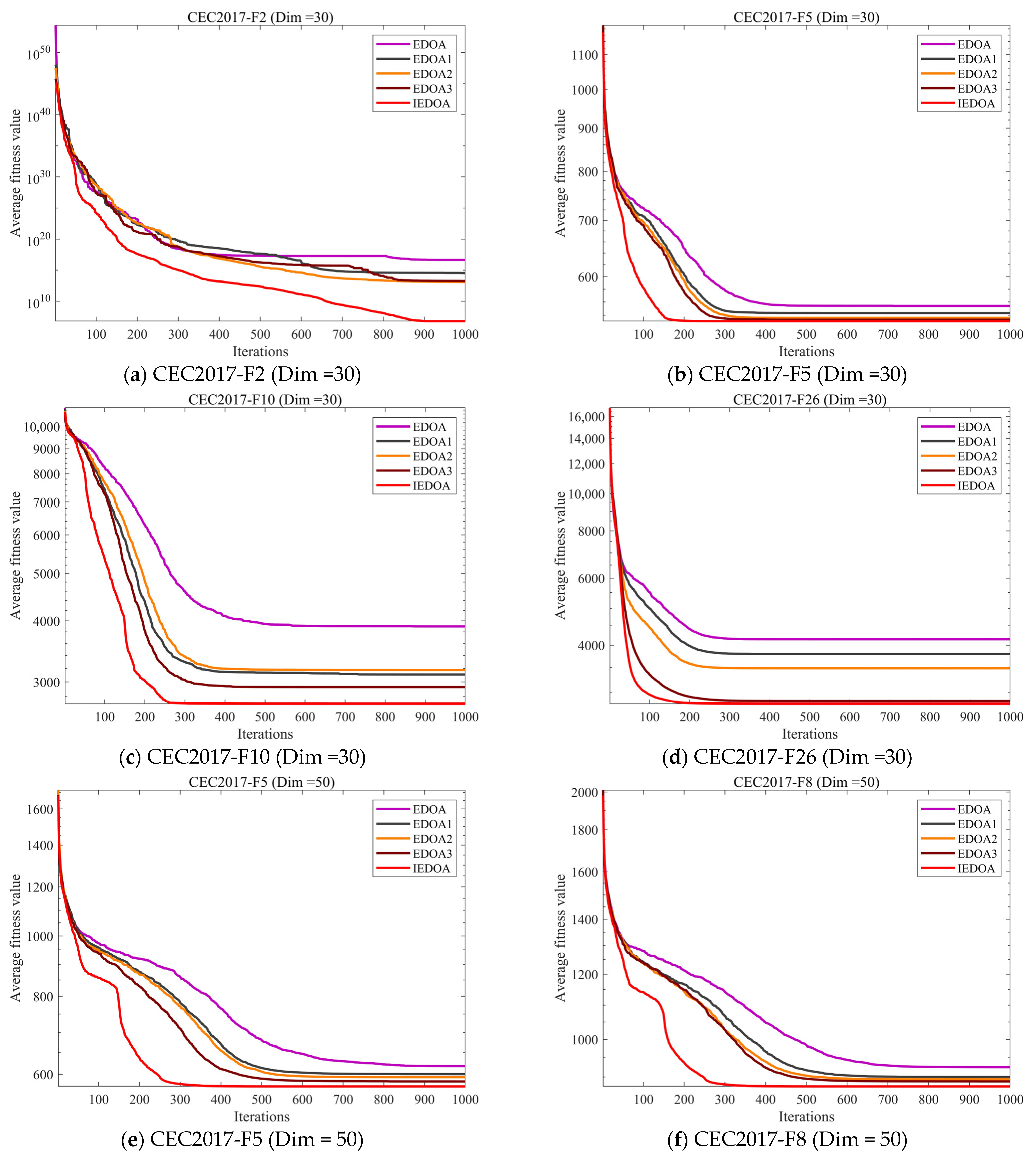
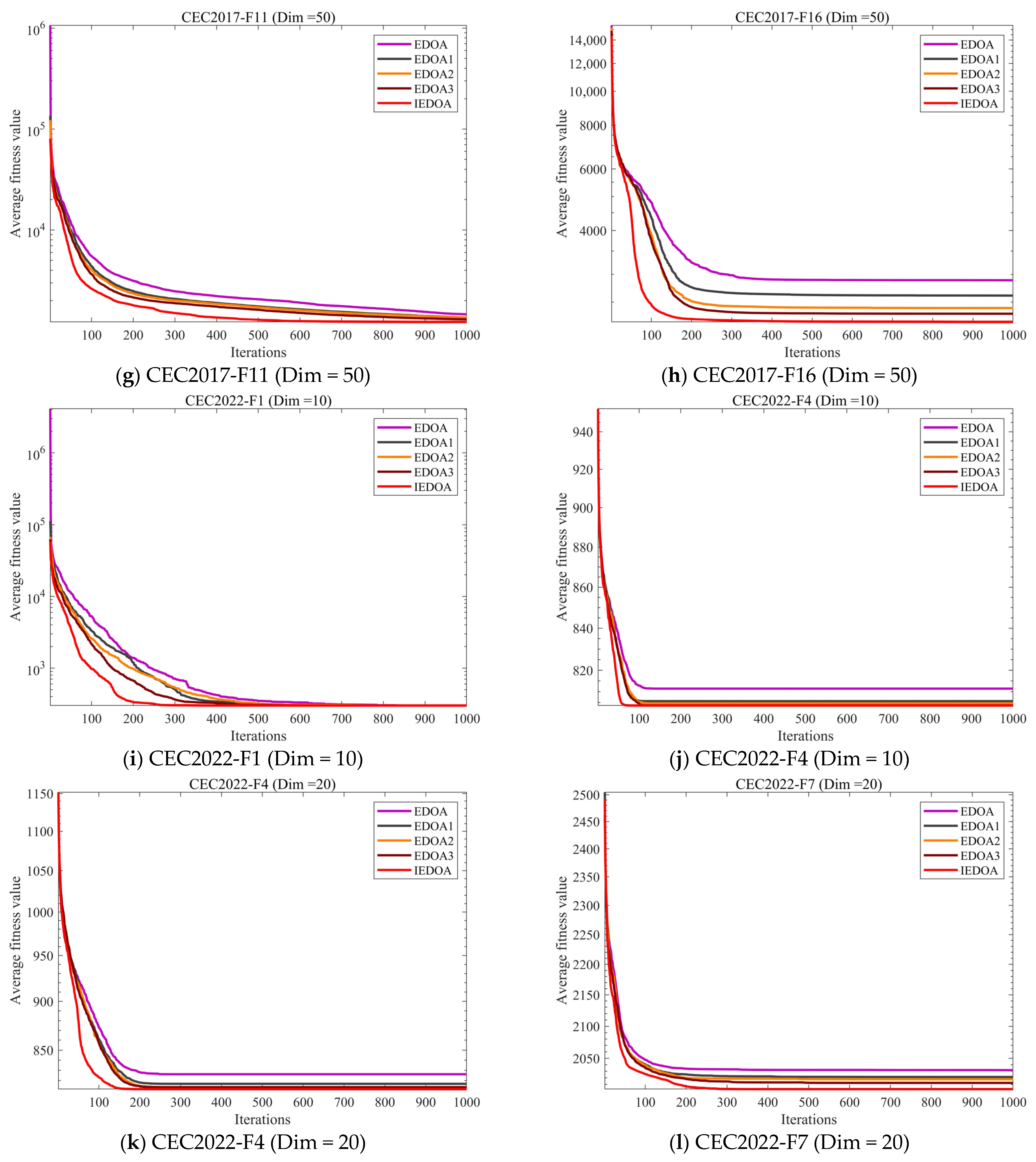
To further elucidate the effectiveness and novelty of the proposed improvement mechanisms, we conducted an ablation study by progressively incorporating three strategies—adaptive activity selection, multi-elite-guided structural evolution, and lifecycle-aware technique updating—into EDOA using the CEC2017 and CEC2022 test suites. Specifically, EDOA1 denotes the standard EDOA augmented with the adaptive activity selection strategy; EDOA2 denotes the standard EDOA augmented with the multi-elite-guided structural evolution strategy; and EDOA3 denotes the standard EDOA augmented with the lifecycle-aware strategy. The specific experimental results are illustrated in the accompanying figure.

Figure 10 demonstrates that all three individual improvement strategies enhance the convergence performance of the original EDOA across various test functions to varying degrees, thereby validating the practical effectiveness of the three proposed mechanisms. Specifically, Adaptive Activity Selection aids in improving the targeted allocation of search resources; Multi-Elite-Guided Structural Evolution strengthens the inheritance of high-quality solutions while maintaining population diversity; and Lifecycle-Aware Updating reinforces the dynamic coordination between global exploration during the early stages of the algorithm and local exploitation during the later stages. Furthermore, the complete IEDOA exhibits a faster convergence rate and achieves lower final objective function values across the majority of test curves, outperforming EDOA1, EDOA2, and EDOA3—each of which incorporates only a single improvement module. This indicates the presence of significant synergistic gains among the three strategies: while individual mechanisms can locally boost algorithm performance, only through their organic integration can the balance between exploration and exploitation be more fully realized, thereby significantly enhancing the algorithm’s convergence accuracy, stability, and capability for solving complex problems.

4.7. Parameter Sensitivity Analysis

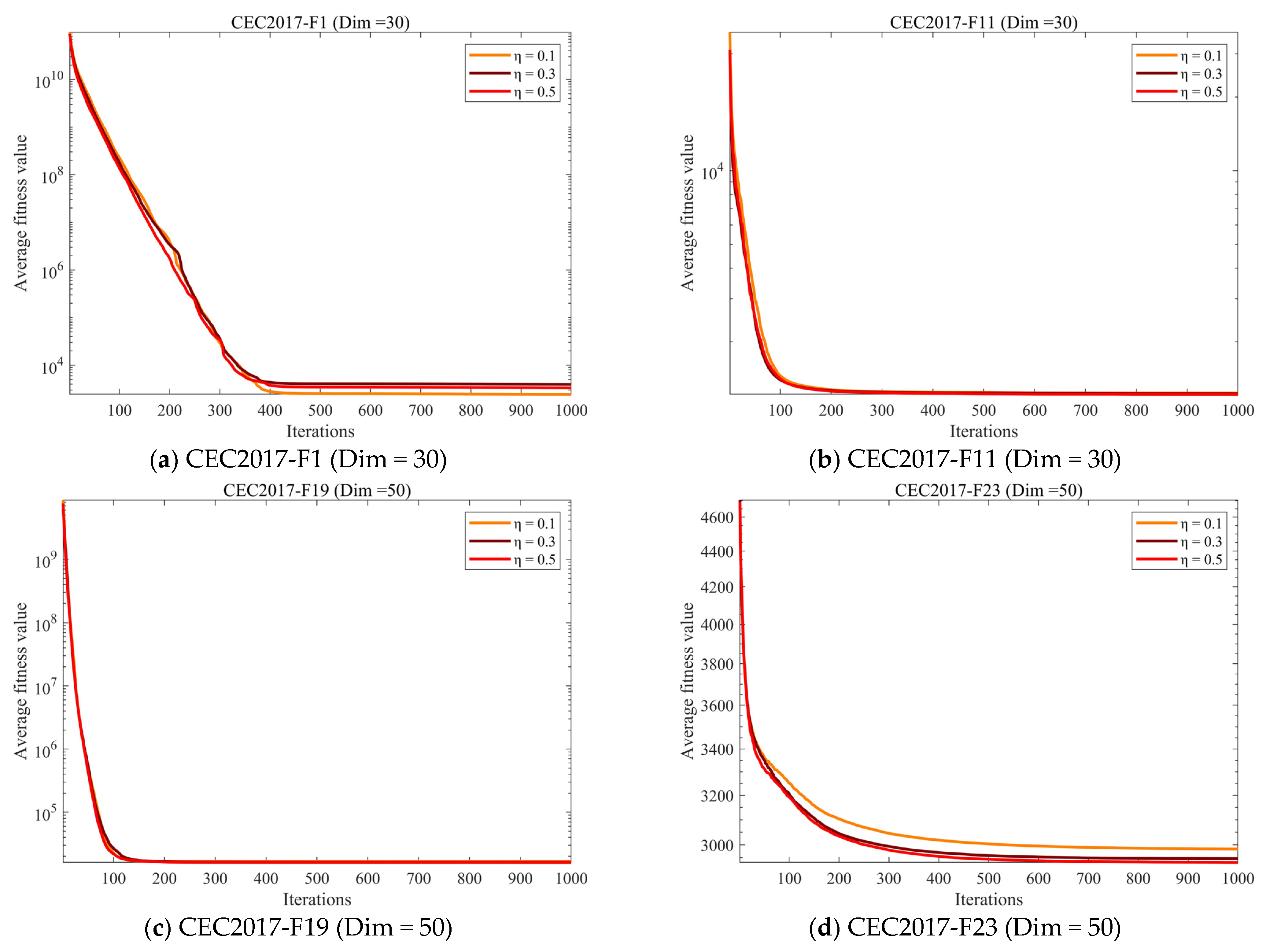
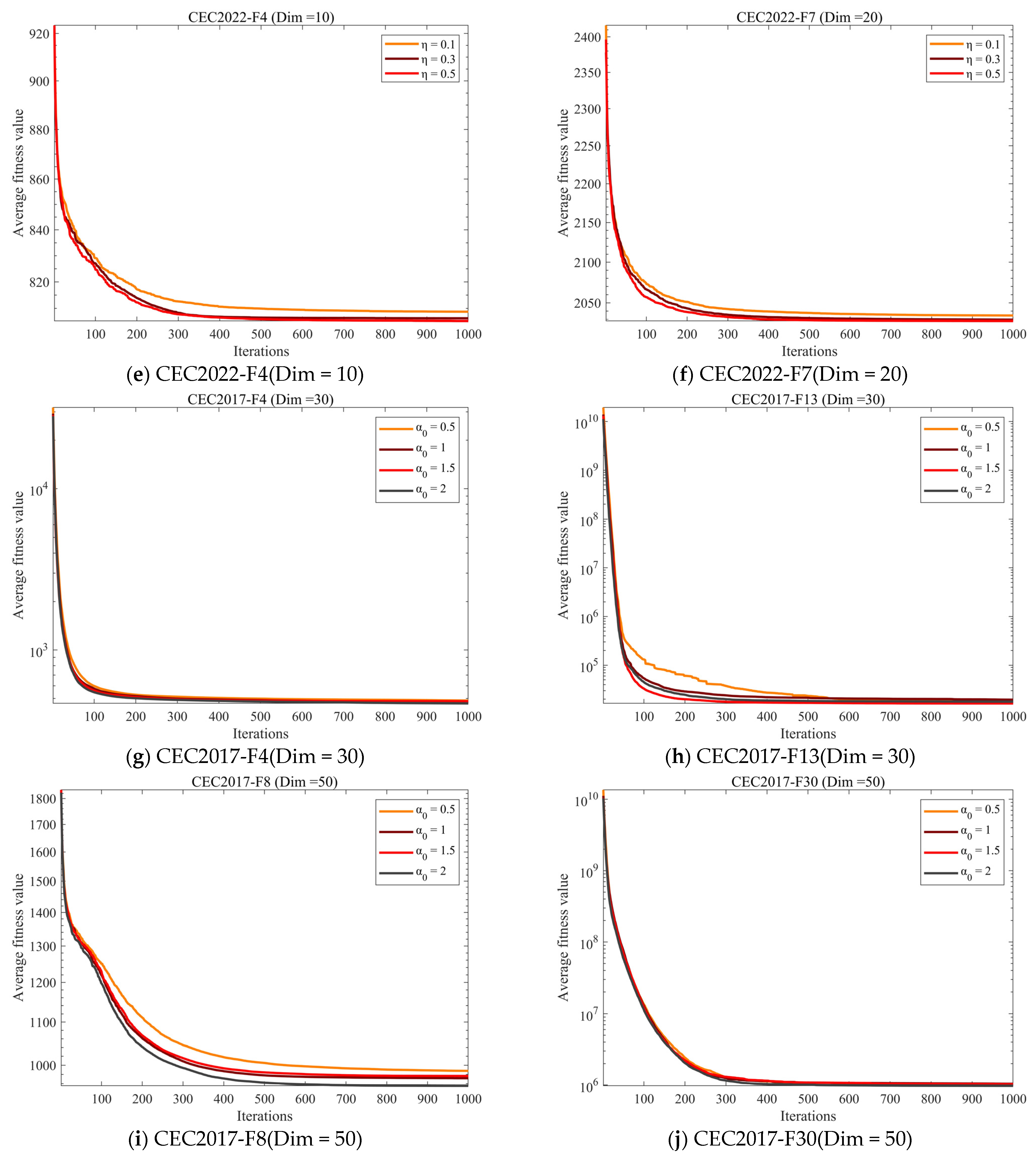
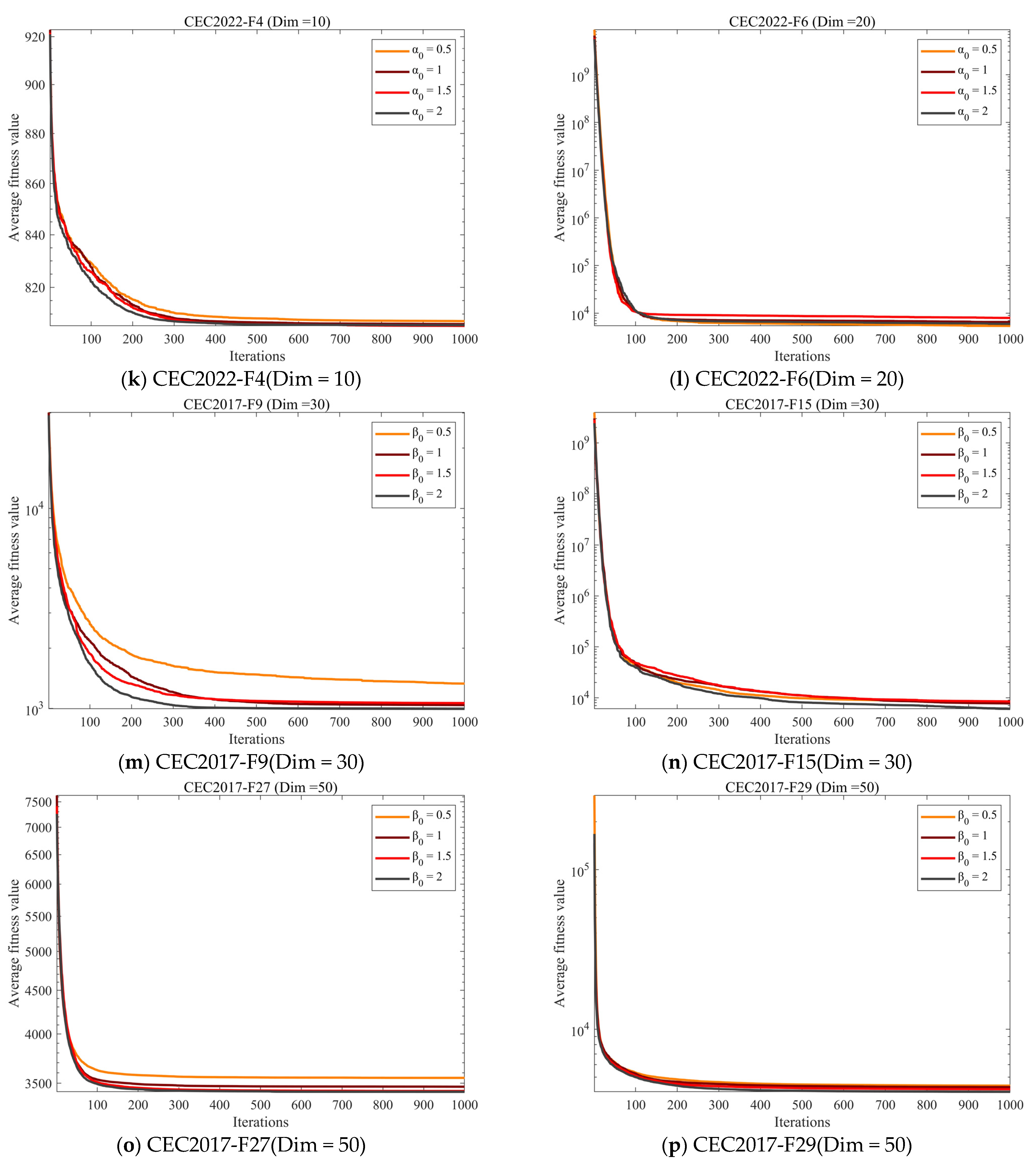
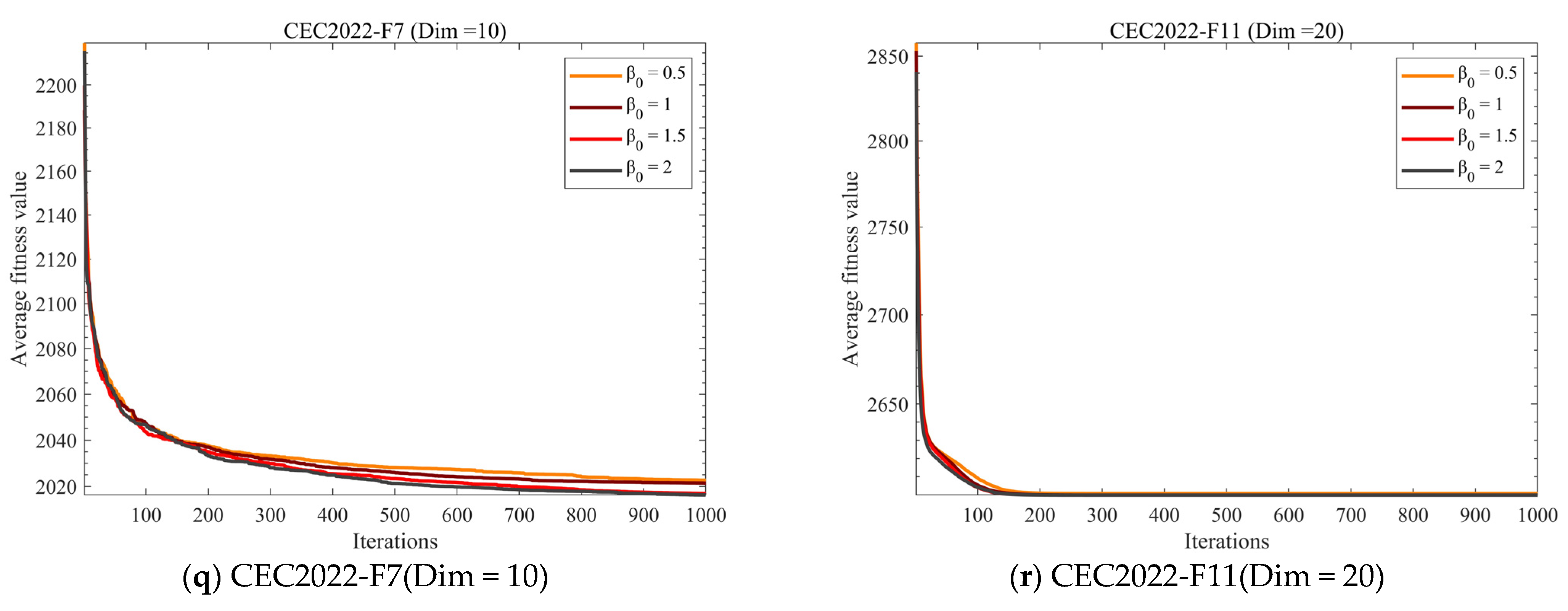
To systematically assess the impact of key algorithm parameters on overall performance—and to validate the rationality and robustness of the selected parameter configuration—this subsection conducts a parameter sensitivity analysis. By incrementally adjusting core parameters across various value ranges while holding other variables constant, the study compares the algorithm’s convergence accuracy and speed on a set of benchmark test functions, thereby elucidating the mechanisms through which individual parameters influence the search process. The experimental results are presented in the accompanying figure.

The parameter sensitivity analysis presented in Figure 11 indicates that IEDOA generally demonstrates robust performance against variations in key parameters: across various test functions and dimensions, the overall trends of the convergence curves for different parameter sets remain consistent, suggesting that the algorithm maintains stable optimization behavior within a reasonable parameter range. At the same time, different parameter values do exert observable effects on both convergence speed and final accuracy; specifically, parameter configurations of moderate intensity typically yield superior results—facilitating a rapid decline in the objective function value during the initial stages while achieving lower and more stable convergence outcomes in the later stages. Conversely, excessively small parameter values tend to diminish the search impetus, resulting in insufficient convergence progress, whereas excessively large values are prone to inducing search fluctuations or stagnation during the latter stages. Synthesizing the results from the various test functions depicted in the figure, it becomes evident that IEDOA’s performance advantages do not hinge upon a single, “acute” parameter point; rather, the algorithm sustains strong performance across a certain range of parameter values. This observation validates the rationality of the adopted settings for the learning rate and lifecycle scheduling parameters, and further substantiates the effectiveness and robustness of the algorithm’s mechanism for balancing exploration and exploitation.

5. IEDOA for Microgrid Dispatch Management

5.1. Microgrid System Configuration

To further verify the practical applicability of the proposed IEDOA, a grid-connected microgrid economic dispatch problem is considered. The microgrid consists of multiple distributed energy resources, including photovoltaic (PV) panels, wind turbines (WT), fuel cells (FC), microturbines (MT), gas generators (GS), battery storage (BT), and power exchange with the main grid. The overall objective of the dispatch problem is to minimize the total operating cost of the microgrid while satisfying power balance and operational constraints.

The scheduling horizon is set to 24 h, and the dispatch interval is 1 h, resulting in 24 decision periods. The renewable energy sources (PV and WT) are treated as non-dispatchable units, and their power outputs are determined according to forecasted generation profiles. In contrast, FC, MT, and GS are controllable generators whose outputs can be adjusted within specified limits. The battery storage system can operate in either charging or discharging mode to balance supply and demand and reduce operating costs. Meanwhile, the microgrid can purchase electricity from or sell electricity to the main grid when necessary.

The power flow relationship of the microgrid can be conceptually expressed as

$$P_{PV}\left(t\right)+P_{WT}\left(t\right)+P_{FC}\left(t\right)+P_{MT}\left(t\right)+P_{GS}\left(t\right)+P_{BT}\left(t\right)+P_{GRID}\left(t\right)=P_{Load}\left(t\right)$$

(16)

where $P_{Load}\left(t\right)$ denotes the load demand at time period $t$. The decision variables of the optimization problem include the output power of controllable units and the grid exchange power over the scheduling horizon:

$$\left\{P_{FC}\right(t),P_{MT}(t),P_{GS}(t),P_{BT}(t),P_{GRID}(t\left)\right\},t=1,\dots ,24$$

(17)

The microgrid considered in this study consists of photovoltaic (PV) generation, wind turbines (WT), fuel cells (FC), microturbines (MT), gas generators (GS), battery storage (BT), and power exchange with the main grid. All components are connected to a common AC bus that supplies the load demand. Renewable sources provide uncontrollable generation based on forecasted profiles, while FC, MT, and GS are dispatchable generators. The battery storage system can charge or discharge to balance supply and demand. The microgrid can also purchase or sell electricity through grid interaction.

5.2. Mathematical Formulation of the Microgrid Economic Dispatch Problem

The economic dispatch problem of the microgrid aims to determine the optimal power outputs of controllable distributed generators, battery storage, and grid interaction over the scheduling horizon so that the total operating cost of the microgrid is minimized while satisfying all operational constraints. The optimization problem consists of 24 consecutive time periods. At each time period, the microgrid must satisfy the electricity demand while minimizing operating cost.

The decision variables of the optimization problem include the power outputs of controllable generation units, the charging/discharging power of the battery storage system, and the power exchanged with the main grid. Renewable sources such as photovoltaic (PV) panels and wind turbines (WT) are treated as non-dispatchable units, and their generation is determined by forecasted profiles.

Let $P_{FC}\left(t\right),P_{MT}\left(t\right),P_{GS}\left(t\right),P_{BT}\left(t\right),P_{GRID}\left(t\right)$ denote the output power of fuel cells, microturbines, gas generators, battery storage, and grid exchange at time period $t$, respectively. The objective of the microgrid dispatch model is to minimize the total operating cost over the scheduling horizon. The objective function can be expressed as

$$F=C_{fuel}+C_{operation}+C_{pollution}+C_{grid}+C_{penalty}$$

(18)

where $C_{fuel}$ represents fuel consumption cost, $C_{operation}$ represents operation and maintenance cost, $C_{pollution}$ denotes pollutant treatment cost, $C_{grid}$ denotes electricity trading cost with the main grid, $C_{penalty}$ represents penalty cost for power imbalance.

(1)

Fuel consumption cost: The fuel cost mainly originates from conventional generation units such as fuel cells, microturbines, and gas generators. The fuel consumption cost over the scheduling horizon is calculated as

$$C_{fuel}=\sum _{t=1}^{24} c\cdot \left({\displaystyle \frac{P_{FC}\left(t\right)}{{\eta }_{FC}}}+{\displaystyle \frac{P_{MT}\left(t\right)}{{\eta }_{MT}}}+{\displaystyle \frac{P_{GS}\left(t\right)}{{\eta }_{GS}}}\right)$$

(19)

where $c$ is the natural gas price and ${\eta }_{FC},{\eta }_{MT},{\eta }_{GS}$ represent the conversion efficiency of the corresponding generators. This term reflects the direct fuel consumption cost associated with power generation.

(2)

Operation and maintenance cost: The operation and maintenance (O&M) cost accounts for the operational expenses required to maintain the distributed energy resources. The O&M cost is calculated as

$$C_{operation}=\sum _{t=1}^{24} \left(K_{FC}{P}_{FC}\left(t\right)+K_{MT}{P}_{MT}\left(t\right)+K_{GS}{P}_{GS}\left(t\right)+K_{PV}{P}_{PV}\left(t\right)+K_{WT}{P}_{WT}\left(t\right)\right)$$

(20)

where $K_i$ represents the O&M cost coefficient of the corresponding generation unit. Although PV and WT are non-dispatchable units, their operation and maintenance costs are still included in the total operating cost.

(3)

Pollution treatment cost: Conventional generators produce pollutant emissions during operation. The pollution treatment cost is introduced to account for the environmental impact of power generation. The pollution treatment cost can be expressed as

$$C_{pollution}=\sum _{t=1}^{24} \sum _i P_i(t)\cdot E_i\cdot C_i$$

(21)

where $E_i$ represents the emission coefficient of generator $i$, $C_i$ represents the treatment cost coefficient for the corresponding pollutant. This term encourages the dispatch model to reduce pollutant emissions by limiting the use of high-emission generation units.

(4)

Electricity trading cost: The microgrid can purchase electricity from the main grid when local generation is insufficient or sell excess electricity when generation exceeds demand. The electricity trading cost is defined as

$$C_{grid}=\sum _{t=1}^{24} P_{GRID}(t)\lambda (t)$$

(22)

where $\lambda \left(t\right)$ represents the time-of-use electricity price, $P_{GRID}\left(t\right)$ represents the power exchanged with the main grid. A positive value of $P_{GRID}\left(t\right)$ indicates electricity purchase from the main grid, while a negative value indicates electricity sold to the grid.

(5)

Power balance penalty: In order to guarantee the balance between electricity supply and demand, a penalty function is introduced to penalize deviations between total generation and load demand.

$$C_{penalty}=\sum _{t=1}^{24} K_{pen}\left|P_{PV}\left(t\right)+P_{WT}\left(t\right)+P_{FC}\left(t\right)+P_{MT}\left(t\right)+P_{GS}\left(t\right)+P_{BT}\left(t\right)+P_{GRID}\left(t\right)-P_{Loud}\left(t\right)\right|$$

(23)

where $K_{pen}$ denotes the penalty coefficient. This penalty term ensures that the total power generation, storage operation, and grid exchange collectively satisfy the load demand of the microgrid.

5.3. Operational Constraints of the Microgrid System

To ensure safe and reliable operation of the microgrid, several operational constraints must be satisfied.

Renewable generation constraint: The outputs of PV and WT are determined by forecasted generation profiles and cannot be directly controlled during dispatch:

$$P_{PV}\left(t\right)=P_{PV,pred}\left(t\right),P_{WT}\left(t\right)=P_{WT,pred}\left(t\right)$$

(24)

Dispatchable generator constraints: The output power of controllable generators must remain within their allowable operating ranges:

$$\begin{gathered} P_{FC,min}\le P_{FC}\left(t\right)\le P_{FC,max} \\ {P}_{MT,min}\le P_{MT}\left(t\right)\le P_{MT,max} \\ {P}_{GS,min}\le P_{GS}\left(t\right)\le P_{GS,max} \end{gathered}$$

(25)

Battery storage constraints: The charging and discharging power of the battery system is limited as

$$P_{BT,min}\le P_{BT}\left(t\right)\le P_{BT,max},$$

(26)

The state of charge (SOC) of the battery is constrained as

$$SO{C}_{min}\le SOC\left(t\right)\le SO{C}_{max}$$

(27)

The SOC dynamics can be expressed as

$$SOC(t+1)=SOC(t)-{\displaystyle \frac{P_{BT}\left(t\right)}{C_{BT}}}$$

(28)

where $C_{BT}$ is the battery capacity. The initial SOC is given as $SOC\left(1\right)=0.4$.

Grid interaction constraint: The power exchanged between the microgrid and the main grid is constrained as

$$-200\le P_{GRID}\left(t\right)\le 200,$$

(29)

where a positive value indicates power purchased from the main grid and a negative value indicates power sold to the grid.

5.4. Parameter Settings

Table 8. Parameter settings for each distributed generation unit.

Power Type	Minimum Power	Maximum Power	Operating Costs	Fuel Costs
PV	0	35	0.0096	0
WT	0	45	0.45	0
FC	0	40	0.02933	0.2435
MT	0	40	0.0419	0.4090
GS	0	40	0.1258	0.6031
BT	−40	40	0.055	0
Grid interaction	−200	200	--	--

summarizes the technical parameters of the distributed generation units and battery storage system used in the microgrid model. These parameters include the minimum and maximum output power, operation costs, and fuel cost coefficients [36,37]. The battery storage system has a capacity of $C_{BT}=40 \mathrm{k}\mathrm{W}$, with SOC limits of $SO{C}_{min}=0.2$ and $SO{C}_{max}=0.8$. The initial SOC is set to 0.4. The natural gas price is set to $2.02\mathrm{\$}/\mathrm{k}\mathrm{g}$, and the penalty coefficient for power imbalance is $20 \mathrm{\$}/\mathrm{k}\mathrm{g}$. Typical daily profiles of load demand, photovoltaic generation, wind power generation, and electricity price are adopted to simulate realistic operating conditions. The dispatch problem is solved over a 24 h scheduling horizon.

5.5. Analysis of Experimental Results

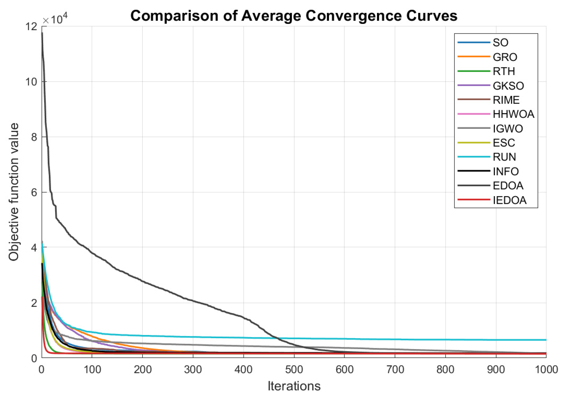
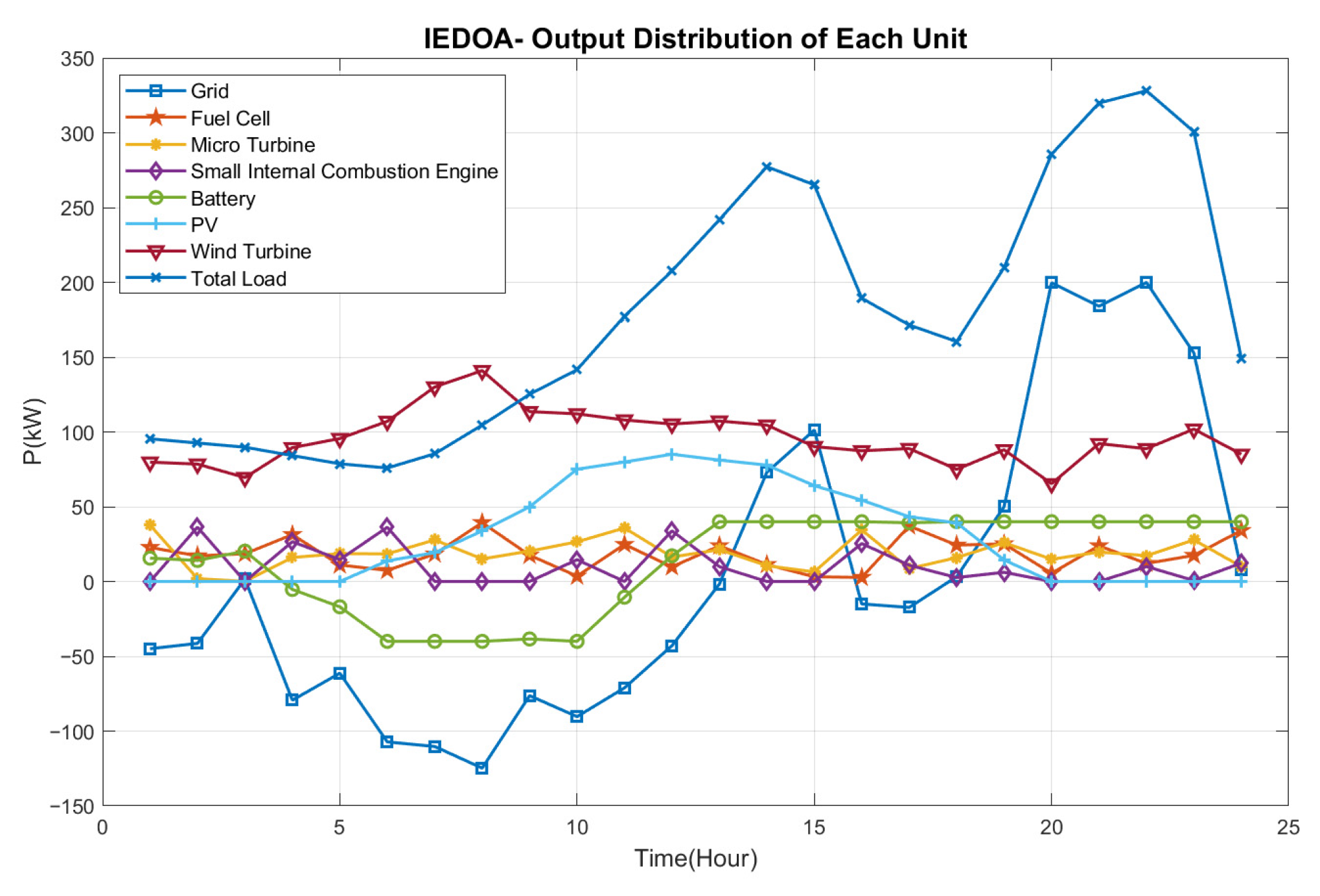
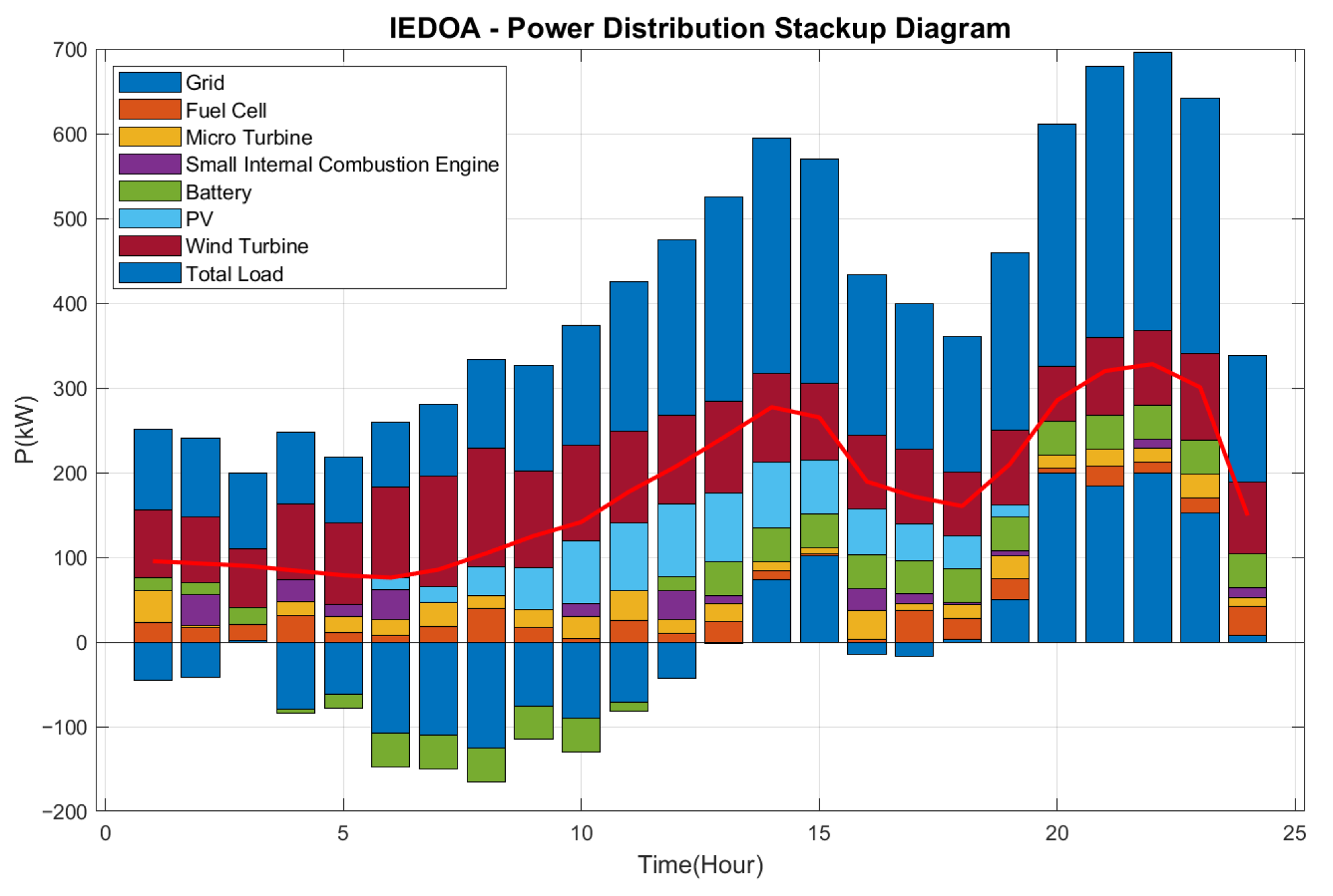
This study considers a grid-connected microgrid system and employs MATLAB as the simulation environment, with GRID representing the main power grid. Regarding algorithm settings, the population size is defined as 50, and the iteration number is set to 1000, whereas the remaining parameters are configured according to the previous description. The maximum allowable power exchange between the microgrid and the utility grid is constrained to 200 kW. The case study is based on a typical daily operating condition from a region in Guangdong Province. To improve comparison reliability and reduce the impact of randomness, each algorithm is executed independently 30 times, followed by statistical analysis of the results. The numerical results are reported in

Table 9. Experimental results by different algorithms.

Algorithms	Max	Min	Mean	Std
SO	2163.61	1556.93	1752.70	138.43
GRO	4148.36	1454.48	1662.91	473.28
RTH	1902.88	1274.56	1554.62	162.18
GKSO	2418.34	1417.95	1872.36	251.71
RIME	2111.39	1470.01	1765.26	137.75
HHWOA	1843.74	1431.53	1670.09	103.62
IGWO	1635.76	1490.97	1568.83	41.31
ESC	1815.34	1531.12	1670.95	72.70
RUN	8372.40	5762.66	6761.83	685.76
INFO	1977.33	1389.42	1612.34	139.86
EDOA	1781.77	1569.87	1676.35	57.76
IEDOA	1606.69	1353.48	1500.54	65.69

, where Max, Min, mean, and std correspond to the maximum, minimum, average, and standard deviation obtained from the 30 runs. Figure 12 depicts the convergence behavior of the objective function for each algorithm, Figure 13 illustrates the output distribution of the units, and Figure 14 displays the stacked bar representation of power allocation.

Table 9 (Experimental Results of Different Algorithms on Microgrid Scheduling Optimization Problems) shows that IEDOA achieved the best overall performance in terms of economy and stability in this engineering scenario: its mean value of 1500.54 over 30 independent runs was the lowest among all algorithms, indicating that IEDOA can obtain the minimum objective function value (i.e., lower operating costs); at the same time, its minimum value of 1353.48 was significantly lower than most of the comparison algorithms, indicating its stronger optimization ability and better optimal solution level. In contrast, the traditional EDOA had a mean value of 1676.35, significantly higher than IEDOA, indicating that the improved strategy brought substantial benefits in practical scheduling problems. Furthermore, from the perspective of stability, IEDOA’s standard deviation of 65.69 was relatively small, indicating lower result fluctuations and stronger robustness; although IGWO had a smaller standard deviation of 41.31, its mean value of 1568.83 was still higher than IEDOA, demonstrating that IEDOA achieved a better balance between “solution quality” and “stability”. It is worth noting that RUN had a mean value of 6761.83 and a standard deviation of 685.76, far higher than other algorithms, indicating that it easily falls into suboptimal solutions and is unstable in this strongly constrained, multi-variable coupled microgrid scheduling problem. Overall, the four indicators of Max/Min/Mean/Std in Table 9 jointly verify that IEDOA can not only obtain lower operating cost objective values in microgrid scheduling optimization tasks but also possesses more reliable convergence stability and engineering applicability.

As shown in Figure 12, there are significant differences in the convergence process of the objective functions of various algorithms in the microgrid scheduling optimization problem. Overall, IEDOA exhibits a faster decrease in the objective function value and a more stable convergence trend during the iteration process. It can obtain a lower objective function value within fewer iterations and maintain continuous improvement, indicating its stronger optimization efficiency and stability in this engineering optimization scenario. In contrast, the convergence curves of some comparison algorithms decrease more slowly or show stagnation and fluctuations in the later stages of iteration, indicating that they are more likely to fall into local optima under complex constraints and multi-variable coupling conditions. In summary, the results in Figure 12 verify that IEDOA can more effectively balance global search and local exploitation in practical scheduling optimization tasks, thus obtaining a better economic operation scheme.

Figure 13 (Output distribution map of each unit) shows that the output distribution of each power generation/energy supply unit during the scheduling period exhibits a distinct division of labor and complementary characteristics: the output of different units changes differently over time, indicating that the optimized scheduling can rationally coordinate various units according to load demand and operating constraints. Overall, the output distribution reflects that the scheduling strategy, while satisfying the system’s supply-demand balance, maximizes the advantages of each unit—for example, units with faster response speeds or stronger regulation capabilities handle fluctuation compensation, while units with lower operating costs or suitable for stable operation handle the base load, thereby reducing overall operating costs and improving system operating stability. This result indicates that the scheduling scheme obtained by IEDOA has good engineering feasibility and economic efficiency, and can achieve the goal of multi-unit collaborative optimization.

As shown in Figure 14 (Power Distribution Stackup Diagram), the power composition of the system throughout the scheduling cycle exhibits a clear superposition relationship, with various power sources, energy storage, and interactive power sources collectively contributing to meet the load demand. It can be observed that the proportion of energy supplied by different energy units varies dynamically at different times: during periods of high or fluctuating load, units with stronger regulatory capabilities (such as energy storage, controllable units, or power interaction with the main grid) contribute more significantly, used for peak shaving, valley filling, and balancing supply and demand; while during periods of relatively stable load, the basic energy supply units maintain a more stable output, thereby improving system operating efficiency. Overall, this superimposed distribution result demonstrates that the proposed method can achieve multi-energy coordination and complementarity, making power distribution more reasonable, smoother, and compliant with operating constraints, further verifying the feasibility and economic efficiency of the scheduling scheme.

Although the results in Figure 12, Figure 13 and Figure 14 and Table 9 demonstrate that IEDOA achieves superior performance in microgrid scheduling, a deeper analysis is required to explain the source of these advantages from the perspective of algorithm–problem matching.

Microgrid economic dispatch is characterized by strong nonlinearity, multi-source coupling, time-varying constraints, and a highly multimodal search landscape, which impose strict requirements on both global exploration and local exploitation capabilities. In this context, the superiority of IEDOA can be attributed to the coordinated effects of its three core mechanisms:

(1)

Performance-adaptive activity selection: In microgrid scheduling, different search behaviors may exhibit varying effectiveness at different stages due to fluctuating load demands and renewable generation uncertainty. The adaptive activity selection mechanism dynamically allocates computational resources based on historical fitness improvement, enabling the algorithm to focus on more productive search patterns. This enhances convergence efficiency and avoids ineffective search steps that are common in fixed or random switching strategies.

(2)

The microgrid dispatch problem often involves multiple competing local optima caused by complex constraints and nonlinear cost functions. The multi-elite guidance mechanism preserves multiple high-quality candidate solutions and integrates their information into the population update process. Compared with single-elite guidance, this strategy effectively maintains population diversity and reduces the risk of premature convergence, thereby improving the algorithm’s ability to explore diverse feasible dispatch schemes.

(3)

Technology lifecycle-aware scheduling mechanism: Microgrid scheduling requires both broad exploration in early stages (to identify feasible regions under constraints) and refined exploitation in later stages (to optimize cost and stability). The lifecycle-aware mechanism introduces a stage-dependent adjustment of exploration and exploitation intensities, which better matches the dynamic requirements of the problem. This allows IEDOA to rapidly locate promising regions and subsequently refine solutions with higher precision.

Overall, the improved performance of IEDOA is not only reflected in numerical results but also arises from its better alignment with the intrinsic characteristics of microgrid scheduling problems, where adaptivity, diversity preservation, and dynamic search balance are critical for achieving high-quality solutions.

It should also be noted that the current microgrid model assumes deterministic inputs for renewable generation and load demand. In practical scenarios, uncertainties such as forecasting errors and market fluctuations may affect the scheduling results, which will be considered in future studies.

6. Conclusions and Future Work

This paper investigates the scheduling and management problem of microgrids, which is a nonlinear, multi-constrained, and strongly coupled optimization task. To address the limitations of the original Enterprise Development Optimization Algorithm (EDOA), including premature convergence and insufficient stability in complex search spaces, an improved version (IEDOA) is proposed. The algorithm incorporates a performance-based adaptive activity selection mechanism, a multi-elite guided evolution strategy, and a lifecycle-aware scheduling mechanism, which collectively enhance the balance between global exploration and local exploitation, as well as improve convergence stability.

Extensive experiments on CEC2017 and CEC2022 benchmark functions demonstrate that IEDOA achieves superior optimization accuracy, convergence speed, and robustness compared with several state-of-the-art algorithms. Statistical analyses using the Wilcoxon rank-sum test and Friedman ranking further confirm the significant and consistent performance advantages of the proposed method across different problem types and dimensional settings.

In addition, the application to a microgrid economic dispatch model verifies the practical effectiveness of IEDOA. The results show that the proposed algorithm can achieve lower operating costs with stable performance while satisfying system constraints, indicating its strong engineering applicability.

Despite these advantages, several limitations remain. The introduction of multiple adaptive and evolutionary mechanisms increases parameter sensitivity and computational complexity, which may affect performance in real-time or large-scale scenarios. Moreover, the current microgrid model assumes deterministic renewable generation and load demand, which does not fully capture real-world uncertainties. The generalization ability of the algorithm to other complex application domains also requires further validation.

Future work will focus on improving computational efficiency and reducing parameter dependence, as well as extending the proposed approach to stochastic and dynamic optimization environments. Incorporating uncertainty modeling, multi-objective optimization, and large-scale energy system applications will further enhance the practicality and robustness of the algorithm.

References

1. Mbungu, N.T.; Ismail, A.A.; AlShabi, M.; Bansal, R.C.; Elnady, A.; Hamid, A.K. Control and Estimation Techniques Applied to Smart Microgrids: A Review. Renew. Sustain. Energy Rev. 2023, 179, 113251. [Google Scholar] [CrossRef]
2. Guo, S.; Song, Y.; Wu, Y.; Hu, J.; Lu, J.; Wang, C.; Jia, Z.; Hua, L. Microscopic Mechanism of Enhanced Strength-Plasticity Synergy in Pre-Damaged TC11 Titanium Alloys via Novel Electroshock Treatment. J. Alloys Compd. 2026, 1052, 186139. [Google Scholar] [CrossRef]
3. Wu, X.; Wang, H.; Zhang, Y.; Zou, B.; Hong, H. A Tutorial-Generating Method for Autonomous Online Learning. IEEE Trans. Learn. Technol. 2024, 17, 1532–1541. [Google Scholar] [CrossRef]
4. Ahmad, S.; Shafiullah, M.; Ahmed, C.B.; Alowaifeer, M. A Review of Microgrid Energy Management and Control Strategies. IEEE Access 2023, 11, 21729–21757. [Google Scholar] [CrossRef]
5. Wu, X.; Dong, J.; Bao, W.; Zou, B.; Wang, L.; Wang, H. Augmented Intelligence of Things for Emergency Vehicle Secure Trajectory Prediction and Task Offloading. IEEE Internet Things J. 2024, 11, 36030–36043. [Google Scholar] [CrossRef]
6. Mohammed, A.; Ghaithan, A.M.; Al-Hanbali, A.; Attia, A.M. A Multi-Objective Optimization Model Based on Mixed Integer Linear Programming for Sizing a Hybrid PV-Hydrogen Storage System. Int. J. Hydrogen Energy 2023, 48, 9748–9761. [Google Scholar] [CrossRef]
7. Fan, D.; Zhu, X.; Xiang, Z.; Lu, Y.; Quan, L. Dimension-Reduction Many-Objective Optimization Design of Multimode Double-Stator Permanent Magnet Motor. IEEE Trans. Transp. Electrif. 2024, 11, 1984–1994. [Google Scholar] [CrossRef]
8. Lü, X.; He, S.; Xu, Y.; Zhai, X.; Qian, S.; Wu, T.; Wangpei, Y. Overview of Improved Dynamic Programming Algorithm for Optimizing Energy Distribution of Hybrid Electric Vehicles. Electr. Power Syst. Res. 2024, 232, 110372. [Google Scholar] [CrossRef]
9. Zhang, J.; Qi, H.; Wu, J.J.; Mao, X.; Zhang, H.; Amin, N.; Xu, F.; Dong, C.; Wang, C.; Wang, P. Disposable Peptidoglycan-Specific Biosensor for Noninvasive Real-Time Detection of Broad-Spectrum Gram-Positive Bacteria in Exhaled Breath Condensates. Anal. Chem. 2024, 96, 9817–9825. [Google Scholar] [CrossRef]
10. Liu, D.; Shen, Q.; Liu, J. The Health-Wealth Gradient in Labor Markets: Integrating Health, Insurance, and Social Metrics to Predict Employment Density. Computation 2026, 14, 22. [Google Scholar] [CrossRef]
11. Yan, J.; Cheng, Y.; Zhang, F.; Li, M.; Zhou, N.; Jin, B.; Wang, H.; Yang, H.; Zhang, W. Research on Multimodal Techniques for Arc Detection in Railway Systems with Limited Data. Struct. Health Monit. 2025, 14759217251336797. [Google Scholar] [CrossRef]
12. Wang, H.; Song, Y.; Yang, H.; Liu, Z. Generalized Koopman Neural Operator for Data-Driven Modelling of Electric Railway Pantograph-Catenary Systems. IEEE Trans. Transp. Electrif. 2025, 11, 14100–14112. [Google Scholar]
13. Yu, Z.; Si, Z.; Li, X.; Wang, D.; Song, H. A Novel Hybrid Particle Swarm Optimization Algorithm for Path Planning of UAVs. IEEE Internet Things J. 2022, 9, 22547–22558. [Google Scholar] [CrossRef]
14. Kullampalayam Murugaiyan, N.; Chandrasekaran, K.; Manoharan, P.; Derebew, B. Leveraging Opposition-Based Learning for Solar Photovoltaic Model Parameter Estimation with Exponential Distribution Optimization Algorithm. Sci. Rep. 2024, 14, 528. [Google Scholar] [CrossRef] [PubMed]
15. Uzun, Y.; Bilgin, M. Medical Image Enhancement Using War Strategy Optimization Algorithm. Biomed. Signal Process. Control 2025, 106, 107740. [Google Scholar] [CrossRef]
16. Feng, X.; Cui, L.; Ren, D.; Pan, A.; Hong, J. A New Adaptive Robust Multi-Objective Optimization Algorithm for Dispatching of Microgrids Design. Eng. Appl. Artif. Intell. 2025, 159, 111715. [Google Scholar] [CrossRef]
17. Tiwari, V.; Dubey, H.M.; Pandit, M.; Salkuti, S.R. Economic Dispatch in Microgrid with Battery Storage System Using Wild Geese Algorithm. Green Energy Intell. Transp. 2025, 4, 100263. [Google Scholar] [CrossRef]
18. Truong, D.-N.; Chou, J.-S. Metaheuristic Algorithm Inspired by Enterprise Development for Global Optimization and Structural Engineering Problems with Frequency Constraints. Eng. Struct. 2024, 318, 118679. [Google Scholar] [CrossRef]
19. Zhao, D.; Feng, L.; Wang, Y.; Cai, X.; Liu, X. An Improved Enterprise Development Optimizer Based on Labor Migration for Numerical Optimization. Sci. Rep. 2025, 15, 26227. [Google Scholar] [CrossRef] [PubMed]
20. Cai, X.; Wang, W.; Wang, Y. Multi-Strategy Enterprise Development Optimizer for Numerical Optimization and Constrained Problems. Sci. Rep. 2025, 15, 10538. [Google Scholar] [CrossRef]
21. Li, Z.; Liao, Y.; Zhou, H. Improved Enterprise Development Optimization with Historical Trend Updating for High-Precision Photovoltaic Model Parameter Estimation. Mathematics 2026, 14, 121. [Google Scholar] [CrossRef]
22. Wu, G.; Mallipeddi, R.; Suganthan, P.N. Problem Definitions and Evaluation Criteria for the CEC 2017 Competition on Constrained Real-Parameter Optimization; Technical Report; National University of Defense Technology: Changsha, China; Kyungpook National University: Daegu, Republic of Korea; Nanyang Technological University: Singapore, 2017; Volume 9, p. 2017. [Google Scholar]
23. Ahrari, A.; Elsayed, S.; Sarker, R.; Essam, D.; Coello, C.A.C. Problem Definition and Evaluation Criteria for the CEC’2022 Competition on Dynamic Multimodal Optimization; UNSW: Sydney, Australia, 2022; pp. 18–23. [Google Scholar]
24. Hashim, F.; Hussien, A. Snake Optimizer: A Novel Meta-Heuristic Optimization Algorithm. Knowl.-Based Syst. 2022, 242, 108320. [Google Scholar] [CrossRef]
25. Zolfi, K. Gold Rush Optimizer: A New Population-Based Metaheuristic Algorithm. Oper. Res. Decis. 2023, 33, 113–150. [Google Scholar] [CrossRef]
26. Ferahtia, S.; Houari, A.; Rezk, H.; Djerioui, A.; Machmoum, M.; Motahhir, S.; Ait-Ahmed, M. Red-Tailed Hawk Algorithm for Numerical Optimization and Real-World Problems. Sci. Rep. 2023, 13, 12950. [Google Scholar] [CrossRef]
27. Hu, G.; Guo, Y.; Wei, G.; Abualigah, L. Genghis Khan Shark Optimizer: A Novel Nature-Inspired Algorithm for Engineering Optimization. Adv. Eng. Inform. 2023, 58, 102210. [Google Scholar] [CrossRef]
28. Su, H.; Zhao, D.; Heidari, A.A.; Liu, L.; Zhang, X.; Mafarja, M.; Chen, H. RIME: A Physics-Based Optimization. Neurocomputing 2023, 532, 183–214. [Google Scholar] [CrossRef]
29. Su, Y.; Dai, Y.; Liu, Y. A Hybrid Hyper-Heuristic Whale Optimization Algorithm for Reusable Launch Vehicle Reentry Trajectory Optimization. Aerosp. Sci. Technol. 2021, 119, 107200. [Google Scholar] [CrossRef]
30. Nadimi-Shahraki, M.H.; Taghian, S.; Mirjalili, S. An Improved Grey Wolf Optimizer for Solving Engineering Problems. Expert Syst. Appl. 2021, 166, 113917. [Google Scholar] [CrossRef]
31. Ouyang, K.; Fu, S.; Chen, Y.; Cai, Q.; Heidari, A.A.; Chen, H. Escape: An Optimization Method Based on Crowd Evacuation Behaviors. Artif. Intell. Rev. 2024, 58, 19. [Google Scholar] [CrossRef]
32. Ahmadianfar, I.; Heidari, A.A.; Gandomi, A.H.; Chu, X.; Chen, H. RUN beyond the Metaphor: An Efficient Optimization Algorithm Based on Runge Kutta Method. Expert Syst. Appl. 2021, 181, 115079. [Google Scholar] [CrossRef]
33. Ahmadianfar, I.; Heidari, A.A.; Noshadian, S.; Chen, H.; Gandomi, A.H. INFO: An Efficient Optimization Algorithm Based on Weighted Mean of Vectors. Expert Syst. Appl. 2022, 195, 116516. [Google Scholar] [CrossRef]
34. Natarajan, S.; Lipsitz, S.R.; Fitzmaurice, G.M.; Sinha, D.; Ibrahim, J.G.; Haas, J.; Gellad, W. An Extension of the Wilcoxon Rank Sum Test for Complex Sample Survey Data. J. R. Stat. Soc. Ser. C Appl. Stat. 2012, 61, 653–664. [Google Scholar] [CrossRef]
35. Zimmerman, D.W.; Zumbo, B.D. Relative Power of the Wilcoxon Test, the Friedman Test, and Repeated-Measures ANOVA on Ranks. J. Exp. Educ. 1993, 62, 75–86. [Google Scholar] [CrossRef]
36. Cao, L.; Wei, Q. SZOA: An Improved Synergistic Zebra Optimization Algorithm for Microgrid Scheduling and Management. Biomimetics 2025, 10, 664. [Google Scholar] [CrossRef] [PubMed]
37. Cheng, S.; Su, G.C.; Zhao, L.L.; Huang, T.L. Dynamic Dispatch Optimization of Microgrid Based on a QS-PSO Algorithm. J. Renew. Sustain. Energy 2017, 9, 045505. [Google Scholar] [CrossRef]
Figure 1. The flowchart of EDOA.
Symmetry 18 00601 g001
Figure 2. Schematic diagram of performance-based adaptive activity selection mechanism.
Symmetry 18 00601 g002
Figure 3. Schematic diagram of multi-elite guided structural evolution strategy.
Symmetry 18 00601 g003
Figure 4. Exploring Technology Lifecycle Awareness—Utilizing Scheduling Mechanisms.
Symmetry 18 00601 g004
Figure 5. The flowchart of IEDOA.
Symmetry 18 00601 g005
Figure 6. Convergence Performance of Different Algorithms on the CEC2017 Test Set.
Symmetry 18 00601 g006aSymmetry 18 00601 g006b
Figure 7. Boxplot analysis of algorithm performance on the CEC2017 test set.
Symmetry 18 00601 g007aSymmetry 18 00601 g007b
Figure 8. Convergence Performance of Different Algorithms on the CEC2022 Test Set.
Symmetry 18 00601 g008aSymmetry 18 00601 g008b
Figure 9. Boxplot analysis of algorithm performance on the CEC2022 test set.
Symmetry 18 00601 g009
Figure 10. Results of Ablation Experiments.
Symmetry 18 00601 g010aSymmetry 18 00601 g010b
Figure 11. Results of Parameter Sensitivity Analysis.
Symmetry 18 00601 g011aSymmetry 18 00601 g011bSymmetry 18 00601 g011cSymmetry 18 00601 g011d
Figure 12. Convergence curves of the objective function values for each algorithm.
Symmetry 18 00601 g012
Figure 13. Output distribution map of each unit.
Symmetry 18 00601 g013
Figure 14. Power Distribution Stackup Diagram.
Symmetry 18 00601 g014