An Improved Multi-Objective Moth Flame Optimization Algorithm Based on r-Domination and Its Application in Parameter Optimization of Multi-Spacecraft Attitude Control

Abstract

To solve the multi-objective optimization problem (MOP) for parameter optimization of a multiple spacecraft attitude controller, an improved multi-objective moth–flame optimization algorithm based on r-domination (rIMOMFO) is proposed. In rIMOMFO, Cauchy mutation is utilized to produce flames that can improve the global search ability. Based on the difference of fitness variance between the two generations of moths, a hybrid mutation strategy is used to perturb moths, which can improve the population diversity of moths. Meanwhile, an adaptive parameter is applied to the moth position update mechanism, which can further balance the exploitation and exploration. In addition, r-domination is used to lead the search toward the preference of the decision maker. The effectiveness of the rIMOMFO is verified using test problems (CF, UF and WFG). Finally, rIMOMFO is used to optimize the parameters of a distributed cooperative controller for multiple spacecraft attitudes. The experimental topological structure is symmetrical. The results show that the optimized controller can accelerate the convergence speed and improve the control accuracy.

1. Introduction

Cooperative control techno [logy of multiple spacecraft has a wide and important application in the development of national defense and science technology [1,2,3,4]. Distributed synthetic aperture radar, three-dimensional imaging and other earth observation tasks involving multiple spacecraft require each spacecraft to point to a specific position on the earth. The above situation must ensure that each spacecraft can track the preset attitude trajectory [5]. Especially for multiple spacecraft tasks, rapidly tracking accuracy and stability is a very challenging problem.

The distributed cooperative control system for multiple spacecraft attitudes is a multi-variable, strong coupling and nonlinear composite system. For the last several years, many researchers have studied the attitude distributed cooperative control systems of multiple spacecraft. In [6], an adaptive control method is designed to realize the coordinated attitude tracking control of a group of spacecraft without speed. In [7], according to the problem of finite time and velocity free attitude coordinated control in undirected communication graph, a continuous distributed finite time spacecraft attitude coordinated control law without angular velocity measurement is designed, which ensures a group of spacecraft can track a common time-varying reference attitude in a limited time. In [8], to settle the problem of relative position coordination control of a spacecraft formation flight under an undirected communication diagram, a new event-based coordinated control scheme is proposed that reduces the communication load. In addition, researchers have also studied the problem of multi-spacecraft preset time event-triggered attitude consensus control with time-varying state constraints, collaborative control problems, distributed finite-time attitude coordination control of spacecraft formation under multiple constraints on angular velocity and control torque, and spacecraft cluster cooperative obstacle avoidance control [9,10,11,12]. However, different controller parameters produce different control results for the cooperative control of multiple spacecraft. It is an MOP of how to find the appropriate controller parameters and optimize the performance of such multiple spacecraft when there are multiple constraints in the real system.

In recent years, scholars have conducted extensive research on traditional mathematical optimization methods and intelligent optimization methods for complex optimization problems [13,14,15]. Related research has been conducted on intelligent optimization methods. The multi-objective evolutionary algorithms (MOEAs) for complex optimization problems have been deeply studied [15,16,17]. With the development of MOEAs, many excellent algorithms were developed, such as non-dominated sorting genetic algorithm II (NSGA-II) [18], the multi-objective evolutionary algorithm based on decomposition (MOEA/D) [19], strength pareto evolutionary algorithm 2 (SPEA2) [20] and non-dominated sorting genetic algorithm III (NSGA-III) [21]. The MOEAs are composed of an evolutionary algorithm and a multi-objective mechanism. Among them, the multi-objective mechanism includes non dominated sorting methods, decomposition-based mechanisms and so on. For large-scale multi-objective problems with large decision variables, ref. [22] proposes an evolutionary strategy based on a two-stage accelerated search optimizer. Specifically, in the first stage, a convergence optimizer was designed, and in the second stage, a reverse learning differential optimization algorithm was used as the diversity optimizer. For the Constrained Multi-Objective Optimization Problem with Deception Constraints (DCMOP), ref. [23] proposes a novel evolutionary multitasking algorithm using a collaborative multi-step mutation strategy. This algorithm transforms DCMOP into a multitask optimization problem, where the main task is the original DCMOP and the auxiliary task aims to provide effective support for the main task. Specifically, the designed collaborative multi-step mutation strategy includes two contributions to addressing deception constraints. For problems with multiple objectives, strong constraints, large-scale, and mixed variables, ref. [24] proposes a multitask and multi-objective optimization framework that combines evolutionary algorithms and mathematical programming. In this framework, the main task uses an evolutionary algorithm with global search capability to solve multi-objective optimization problems. Auxiliary tasks utilize mathematical programming methods with robust linear constraint handling capabilities to solve multiple weighted single objective optimization problems. In addition, swarm-intelligence-based search algorithms for multi-objective optimization have also been developed and applied to a variety of multi-objective optimization problems [25,26,27].

Since the 1950s, inspired by the laws of biological evolution and optimization phenomena in nature, many intelligent optimization algorithms have been proposed, such as particle swarm optimization (PSO) [28] and genetic algorithm (GA) [29]. The differential evolution (DE) [30] algorithm appeared earlier, but there are many variants that can be utilized to solve different problems. In the past two decades, meta-heuristic algorithms have attracted widespread attention, such as Coyote Optimization Algorithm (COA) [31], Sand Cat Swarm Optimization (SCSO) [32], firefly algorithm (FA) [33], Equilibrium optimizer (EO) [34], Heap-based Optimizer algorithm (HBOA) [35], Cuckoo Search (CS) [36], Sine Cosine Algorithm (SCA) [37], Bacterial Foraging Optimization algorithm (BFO) [38], Barnacles Mating Optimizer (BMO) [39] and moth–flame optimization (MFO) [40].

These intelligent optimization algorithms are used to solve multi-objective optimization problems, such as PSO [41], Whale Optimization Algorithm [42], Grey Wolf Optimization (GWO) [43], CS [44] and Fish Algorithm (FA) [45]. It is worth noting that the MFO is effective in solving some optimization problems [46], but it can become stuck in bad local optima because it focuses on exploitation rather than exploration [47].

To solve the above problems, an improved moth–flame optimization (IMFO) algorithm is proposed. In IMFO, new moth position updating and flame generation mechanisms are designed. Cauchy mutation is utilized to produce flames that lead the moths to their updated positions; a hybrid mutation operator is used to perturb the positions of the moths. Among them, variations in the number of flames and moths can be dynamically adjusted by calculating the difference of fitness variance between the two generations of moths. In addition, an adaptive parameter is applied to the moth position update mechanism to further balance the exploitation and exploration. We combine IMFO with r-dominated sorting to produce rIMOMFO. Moreover, rIMOMFO is utilized to solve the MOP of parameter optimization for a multiple spacecraft attitude controller. To sum up, the main contributions of this paper are as follows:

(1)

Cauchy mutation is utilized to produce flames that lead the moths to their updated positions; a hybrid mutation operator is used to perturb the positions of the moths. Among them, variations in the number of flames and moths can be dynamically adjusted by calculating the difference of fitness variance between the two generations of moths. In addition, an adaptive parameter is applied to the moth position update mechanism to further balance exploitation and exploration.

(2)

The IMFO and r-dominated sorting are combined to produce a multi-objective evolutionary algorithm called rIMOMFO. rIMOMFO is evaluated by benchmark test problems (CF, UF and WFG). The results show that the rIMOMFO algorithm is feasible and effective.

(3)

The rIMOMFO algorithm is used to optimize the parameters of a distributed cooperative controller for multiple spacecraft attitudes. The results show that the optimized controller can improve the control accuracy and accelerate the convergence speed.

The rest of the paper is organized as follows: In Section 2, a multi-objective optimization model of multiple spacecraft attitude distributed cooperative control is established. In Section 3, the rIMOMFO is discussed in detail. In Section 4, the benchmark problems are utilized to test the performance of the rIMOMFO algorithm and how it compares with other algorithms. The rIMOMFO is used to optimize the control parameters of the attitude cooperative controller for multiple spacecraft in Section 5. In Section 6, the conclusions and future works of this study are given.

2. Problem Formulation

2.1. System Description

In this paper, the Modified Rodrigues Parameters (MRPs) [48] are utilized to describe the rigid body attitude motion of each spacecraft. The dynamic equations of the $i(i=1,2,\cdots ,m)$ spacecraft are as follows:

$$\begin{array}{c}\hfill \left\{\begin{array}{c}{\dot{\mathit{\sigma }}}_i=G_i\left({\mathit{\sigma }}_i\right){\mathit{\omega }}_i\hfill \\ {\mathit{J}}_i{\dot{\mathit{\omega }}}_i=-{\mathit{\omega }}_i^{\times }{\mathit{J}}_i{\mathit{\omega }}_i+{\mathit{u}}_i+{\mathit{\epsilon }}_i\hfill \end{array}\right.\end{array}$$

(1)

where ${\mathit{\sigma }}_i={\left[{\sigma }_{i1},{\sigma }_{i2},{\sigma }_{i3}\right]}^T$ represents the ith spacecraft attitude, ${\mathit{\omega }}_i={\left[{\omega }_{i1},{\omega }_{i2},{\omega }_{i3}\right]}^T$ is the angular velocity of the ith spacecraft body coordinate system relative to the inertial coordinate system and ${\mathit{\omega }}_i^{\times }$ denotes a skew-symmetric matrix of ${\mathit{\omega }}_i$, which is given in Equation (2). ${\mathit{u}}_i={\mathit{u}}_{ci}+{\mathit{u}}_{fi}$ is the actual input torque, ${\mathit{u}}_{ci}$ is the expected input torque of the spacecraft (to be designed) and ${\mathit{u}}_{fi}$ is the actuator fault, where the fault is expressed as deviation fault and efficiency fault. ${\mathit{u}}_{fi}={\mathit{f}}_{ai}+\left({\Xi }_i-\mathit{I}\right){\mathit{u}}_{ci}$, ${\mathit{f}}_{ai}$ is the actuator deviation fault and ${\mathit{f}}_{ai}$ is bounded; ${\Xi }_i=diag\left\{{\Xi }_{i1},{\Xi }_{i2},\right.\left.{\Xi }_{i3}\right\}$ is the efficiency factor of the actuator and $0<{\Xi }_{ij}\le 1$, $j=1,2,3$. When ${\Xi }_{ij}=1$, the actuator of the ith spacecraft is in a healthy state; when ${\Xi }_{ij}=0$, the actuator of the ith spacecraft fails completely; when $0<{\Xi }_{ij}\le 1$, there is partial failure of the actuator of the ith spacecraft. ${\mathit{\epsilon }}_i\in R^3$ is the external interference torque, $G_i={\displaystyle \frac{1}{2}}\left[{\displaystyle \frac{1-{\mathit{\sigma }}_i^T{\mathit{\sigma }}_i}{2}}{\mathit{I}}_3+{\mathit{\sigma }}_i^{\times }+{\mathit{\sigma }}_i^T{\mathit{\sigma }}_i\right]$, ${\mathit{I}}_3$ is the unit matrix of order 3, ${\mathit{\sigma }}_i^{\times }$ is the skew-symmetric matrix of ${\mathit{\sigma }}_i$ and ${\mathit{J}}_i\in R^{3\times 3}$ is the moment of inertia.

$$\begin{array}{c}\hfill {\mathit{\omega }}^{\times }=\left[\begin{array}{ccc}0& -{\omega }_3& {\omega }_2\\ {\omega }_3& 0& -{\omega }_1\\ -{\omega }_2& {\omega }_1& 0\end{array}\right]\end{array}$$

(2)

According to reference [48], the Euler–Lagrange equation of multiple spacecraft kinematics is obtained as follows:

$$\begin{array}{c}\hfill {\mathit{M}}_i\left(q_i\right){\ddot{q}}_i+{\mathit{C}}_i({\mathit{q}}_i,{\dot{\mathit{q}}}_i)={\mathit{u}}_i+{\mathit{\epsilon }}_i\end{array}$$

(3)

where ${\mathit{M}}_i\left({\mathit{q}}_i\right)={\mathit{G}}_i^{-T}\left({\mathit{q}}_i\right){\mathit{J}}_i{\mathit{G}}_i^{-1}\left({\mathit{q}}_i\right)$, ${\mathit{C}}_i({\mathit{q}}_i,{\dot{\mathit{q}}}_i)=-{\mathit{G}}_i^{-T}\left({\mathit{q}}_i\right){\left({\mathit{J}}_i{\mathit{G}}_i^{-1}\left({\mathit{q}}_i\right){\dot{\mathit{q}}}_i\right)}^{\times }{\mathit{G}}_i^{-1}\left({\mathit{q}}_i\right)-{\mathit{G}}_i^{-T}\left({\mathit{q}}_i\right){\mathit{J}}_i{\mathit{G}}_i^{-1}\left({\mathit{q}}_i\right){\dot{\mathit{G}}}_i\left({\mathit{q}}_i\right)\times {\mathit{G}}_i^{-1}\left({\mathit{q}}_i\right)$.

2.2. Distributed Coordinative Controller Based on Super Twisting and an Integral Sliding Surface

To cause the attitude of multiple spacecraft to track the preset trajectory quickly with external disturbance and actuator failure, a distributed cooperative controller based on super twisting and an integral sliding mode surface is designed.

Defining $x_{i,1}=q_i,x_{i,2}={\dot{q}}_i$, the kinematics Equation (3) of the ith spacecraft is transformed into

$$\begin{array}{c}\hfill \left\{\begin{array}{c}{\dot{x}}_{i,1}=x_{i,2}\hfill \\ {\dot{x}}_{i,2}=f_i(x_{i,1},x_{i,2})+g_i\left(x_{i,1}\right)u_{ci}+d_i\hfill \\ y_i=x_{i,1}\hfill \end{array}\right.\end{array}$$

(4)

where $f_i(x_{i,1},x_{i,2})=-M_i^{-1}\left(x_{i,1}\right)C_i(x_{i,1},x_{i,2})x_{i,2}$; $g_i\left(x_{i,1}\right)=M_i^{-1}\left(x_{i,1}\right)$; $d_i=M_i^{-1}\left(x_{i,1}\right)({\epsilon }_i+u_{fi})$.

The consensus errors are given

$$\begin{array}{c}\hfill \left\{\begin{array}{c}{\mathit{\chi }}_{i,1}={\sum }_{j=1}^n{a}_{ij}\left({\mathit{x}}_{i,1}-{\mathit{x}}_{j,1}\right)+b_i\left({\mathit{x}}_{i,1}-{\mathit{q}}_0\right)\hfill \\ {\mathit{\chi }}_{i,2}={\sum }_{j=1}^n{a}_{ij}\left({\mathit{x}}_{i,2}-{\mathit{x}}_{j,2}\right)+b_i{\mathit{x}}_{i,2}\hfill \end{array}\right.\end{array}$$

(5)

Define the sliding-mode surface

$$\begin{array}{c}\hfill {\mathit{S}}_i={\mathit{x}}_{i,2}+{\int }_0^t\left(c_{i,1}si{g}^{{\beta }_1}\left({\mathit{\chi }}_{i,1}\left(\tau \right)\right)+c_{i,2}si{g}^{{\beta }_2}\left({\mathit{\chi }}_{i,2}\left(\tau \right)\right)\right)d\tau \end{array}$$

(6)

where ${\mathbf{S}}_i={\left[S_{i,1},S_{i,2},S_{i,3}\right]}^T$, ${\beta }_1={\displaystyle \frac{{\beta }_2}{2-{\beta }_2}}$, ${\beta }_2\in \left(0,1\right)$, $c_{i,1}>0$, $c_{i,2}>0$, and satisfy that polynomial ${\lambda }^2+c_{i,2}\lambda +c_{i,1}$ is Hurwitz, $i=1,2,\cdots ,m$.

Based on reference [49], the distributed consensus controller is designed as

$$\begin{array}{c}\hfill {\mathit{u}}_{ci}=-{\left(g_i\left({\mathit{x}}_{i,1}\right)\right)}^{-1}\left[{\mathit{u}}_i^{nom}+{\mathit{u}}_i^{sw}\right]\end{array}$$

(7)

$$\begin{array}{c}\hfill {\mathit{u}}_i^{nom}={\mathit{f}}_i({\mathit{x}}_{i,1},{\mathit{x}}_{i,2})+{\widehat{d}}_i+c_{i,1}si{g}^{{\beta }_1}\left({\mathit{\chi }}_{i,1}\right)+c_{i,2}si{g}^{{\beta }_2}\left({\mathit{\chi }}_{i,2}\right)\end{array}$$

(8)

$$\begin{array}{c}\hfill {\mathit{u}}_i^{sw}={\delta }_{i,1}{\varphi }_i\left({\mathit{S}}_i\right)-{\int }_0^t{\dot{z}}_i\left({\mathit{S}}_i\right)d\tau \end{array}$$

(9)

where ${\mathit{\varphi }}_i\left({\mathit{S}}_i\right)={\mu }_{i,1}si{g}^{{\displaystyle \frac{1}{2}}}\left({\mathit{S}}_i\right)+{\mu }_{i,2}{\mathit{S}}_i$, ${\dot{z}}_i\left({\mathit{S}}_i\right)=-{\delta }_{i,2}\left({\displaystyle \frac{{\mu }_{i,1}^2}{2}}si{g}^0\left({\mathit{S}}_i\right)+{\mu }_{i,2}^2{\mathit{S}}_i+{\displaystyle \frac{3}{2}}{\mu }_{i,1}{\mu }_{i,2}si{g}^{{\displaystyle \frac{1}{2}}}\left({\mathit{S}}_i\right)\right)=-{\delta }_{i,2}{\mathsf{\Gamma }}_i{\varphi }_i\left({\mathit{S}}_i\right)$, with ${\mathsf{\Gamma }}_i={\displaystyle \frac{{\mu }_{i,1}}{2}}diag\left\{{\left|S_{i,1}\right|}^{-{\displaystyle \frac{1}{2}}},{\left|S_{i,2}\right|}^{-{\displaystyle \frac{1}{2}}},{\left|S_{i,3}\right|}^{-{\displaystyle \frac{1}{2}}}\right\}+{\mu }_{i,2}{\mathit{I}}_3$, ${\delta }_{i,1}>0$, ${\delta }_{i,2}>0$, ${\mu }_{i,1}>0$ and ${\mu }_{i,2}>0$ are constants. ${\widehat{d}}_i$ is the estimation of lumped system interference $d_i$. For the ith spacecraft, the disturbance observer is designed as

$$\begin{array}{c}\hfill \left\{\begin{array}{c}{\dot{\widehat{x}}}_{i,2}=f_i(x_{i,1},x_{i,2})+g_i\left(x_{i,1}\right)u_{ci}+r_{i}si{g}^{{\gamma }_i}\left(e_i\right)+{\widehat{d}}_i\hfill \\ {\dot{\widehat{d}}}_i={\eta }_{i}sign\left({\mathbf{\sigma }}_{di}\right)+{\widehat{\alpha }}_{i}sign\left({\mathbf{\sigma }}_{di}\right)\hfill \end{array}\right.\end{array}$$

(10)

where ${\eta }_i>0$, ${\gamma }_i\in \left(0,1\right)$, ${\widehat{\alpha }}_i$ is the estimate of ${\alpha }_i$, ${\mathbf{\sigma }}_{di}={\dot{e}}_i+r_{i}si{g}^{{\gamma }_i}\left(e_i\right)$ and $e_i=x_{i,2}-{\widehat{x}}_{i,2}$.

2.3. The MOP Formulation for the Attitude Control of Multiple Spacecraft

To make the designed controller improve the control accuracy and accelerate the convergence speed of the system, in this paper, $f_a$$(a=1,2,3)$ and $f_b$$(b=4,5,6)$ are selected as the two kinds of objective functions, and the detailed description is as follows:

(1) $f_a$ is the adjust time for the three axes of the follower spacecraft to reach the specified accuracy. And it is used to embody the rapidity of the multiple spacecraft cooperative control system.

$$\begin{array}{c}\hfill f_a\left(\mathit{x}\right)=\left\{\begin{array}{cc}{t}_s,\hfill & Ifthefollowercanreachacertainaccuracyinthesettime\hfill \\ t_c,\hfill & otherwise\hfill \end{array}\right.\end{array}$$

(11)

where $t_s$ is adjustment time and $t_c$ is penalty time.

(2) $f_b$ is the root mean square error of the attitude of followers after stabilization. And it is used to embody the stability of the multiple spacecraft cooperative control system.

$$\begin{array}{c}\hfill f_b\left(\mathit{x}\right)=\sqrt{{\displaystyle \frac{1}{N_s}}\sum _{n=1}^{N_s}max\left\{{(q_{i,1}\left(b\right)-q_0\left(b\right))}^2\right\}}\end{array}$$

(12)

where $N_s$ is the sample times after spacecraft stabilization, $i(i=1,2,\cdots ,m)$.

The MOP is to search the minimum value of $f_a$ and $f_b$. And the mathematical expression of the optimization problem in this paper is as follows:

$$\begin{array}{c}\hfill \underset{x\in {\mathsf{\Omega }}^m}{min}\mathit{F}\left(\mathit{x}\right)=\{f_1\left(\mathit{x}\right),f_2\left(\mathit{x}\right),f_3\left(\mathit{x}\right),f_4\left(\mathit{x}\right),f_5\left(\mathit{x}\right),f_6\left(\mathit{x}\right)\}\end{array}$$

(13)

$$\begin{array}{c}\hfill subjectto\\ & 0<{\delta }_{i1}\le 2,0<{\delta }_{i2}\le 2\hfill \\ & 0<{\mu }_{i1}\le 2,0<{\mu }_{i2}\le 2,i=1,2,3,4\hfill \\ & {\beta }_1={\displaystyle \frac{{\beta }_2}{2-{\beta }_2}},{\beta }_2\in \left(0,1\right)\hfill \\ \end{array}$$

(14)

where $\mathit{x}=\left[{\delta }_{11},{\delta }_{21},{\delta }_{31},{\delta }_{41},{\delta }_{12},{\delta }_{22},{\delta }_{32},{\delta }_{42},{\mu }_{11},{\mu }_{21},{\mu }_{31},{\mu }_{41},{\mu }_{12},{\mu }_{22},{\mu }_{32},{\mu }_{42},{\beta }_2\right]$ and ${\mathsf{\Omega }}^m$ is the feasible region, including all controller parameters to be found.

3. Improved Multi-Objective Moth–Flame Algorithm Based on r-Domination (rIMOMFO)

3.1. Moth–Flame Optimization Algorithm and r-Dominance Relationship

3.1.1. Moth–Flame Optimization Algorithm

The MFO algorithm is a population-based swarm intelligence algorithm. Moreover, it is inspired by the horizontal positioning mechanism of the moths in flight [40]. There are two populations in MFO: moths (M) and flames (F). They and their corresponding fitness values are shown below.

$$\mathit{M}=\left[\begin{array}{c}{\mathit{M}}_1\\ {\mathit{M}}_2\\ ⋮\\ {\mathit{M}}_n\end{array}\right]=\left[\begin{array}{ccccc}{m}_{11}& m_{12}& \dots & \dots & m_{1d}\\ m_{21}& m_{22}& \dots & \dots & m_{2d}\\ ⋮& ⋮& ⋮& ⋮& ⋮\\ m_{n1}& m_{n2}& \dots & \dots & m_{nd}\end{array}\right]$$

(15)

$$\mathit{OM}=\left[\begin{array}{c}O{M}_1\\ O{M}_2\\ ⋮\\ O{M}_n\end{array}\right]$$

(16)

$$\mathit{F}=\left[\begin{array}{c}{\mathit{F}}_1\\ {\mathit{F}}_2\\ ⋮\\ {\mathit{F}}_n\end{array}\right]=\left[\begin{array}{ccccc}{f}_{11}& f_{12}& \dots & \dots & f_{1d}\\ f_{21}& f_{22}& \dots & \dots & f_{2d}\\ ⋮& ⋮& ⋮& ⋮& ⋮\\ f_{n1}& f_{n2}& \dots & \dots & f_{nd}\end{array}\right]$$

(17)

$$\mathit{OF}=\left[\begin{array}{c}O{F}_1\\ O{F}_2\\ ⋮\\ O{F}_n\end{array}\right]$$

(18)

where n the population number of moths/flames and d is the number of dimensions. ${OM}_i$ and ${OF}_i$ represent the fitness function value of the corresponding moth ${\mathit{M}}_i=\left[m_{i1},m_{i2},\cdots ,m_{id}\right]$ and ${\mathit{F}}_i=\left[f_{i1},f_{i2},\cdots ,f_{id}\right],i\in \{1,2,\cdots ,n\}$, respectively.

The population of moths is initialized as follows [50]:

$$\begin{array}{c}\hfill m_{ij}={lb}_i+w_j\left({ub}_i-l{b}_i\right)\end{array}$$

(19)

where $j=1,2,\cdots ,d$; $w_j$ is a random number in [0,1]; and ${ub}_i$ and ${lb}_i$ indicate the upper and lower bounds of the i-th variables ($\mathit{ub}=\left[u{b}_1,u{b}_2,\dots ,u{b}_n\right]$, $\mathit{lb}=\left[l{b}_1,l{b}_2,\dots ,l{b}_n\right]$).

The position updating formulas of moths are as follows:

$$\begin{array}{c}\hfill {\mathit{M}}_i(l+1)=\left\{\begin{array}{cc}{\mathit{D}}_i\left(l\right)·e^{bt}·cos2\pi t+{\mathit{F}}_i\left(l\right),\hfill & i\le f_{no}\hfill \\ {\mathit{D}}_i\left(l\right)·e^{bt}·cos2\pi t+{\mathit{F}}_{f_{no}}\left(l\right),\hfill & i>f_{no}\hfill \end{array}\right.\end{array}$$

(20)

where $b=1$; t is a random number in [r,1]; $r=-1+l(-1/L)$; l and L represent the current number and the maximum number of iterations, respectively; $f_{no}$ denotes the number of adaptive flames and is calculated by Equation (19); and ${\mathit{D}}_i$ indicates the distance between the ith flame and its corresponding moth. The formula for ${\mathit{D}}_i$ is as follows:

$$\begin{array}{c}\hfill {\mathit{D}}_i\left(l\right)=\left\{\begin{array}{cc}|{\mathit{F}}_i\left(l\right)-{\mathit{M}}_i\left(l\right)|,\hfill & i\le f_{no}\hfill \\ |{\mathit{F}}_{f_{no}}\left(l\right)-{\mathit{M}}_i\left(l\right)|,\hfill & i>f_{no}\hfill \end{array}\right.\end{array}$$

(21)

Meanwhile, to balance exploration and exploitation, MFO uses the adaptive flame number method to determine the number of flames in each iteration. The mathematical expression is as follows:

$$\begin{array}{c}\hfill f_{no}=round(n-{\displaystyle \frac{l(n-1)}{L}})\end{array}$$

(22)

3.1.2. r-Dominance Relation

The r-dominance (reference-solution-based dominance) is the fusion of the Pareto dominance principle and the reference point method (RPM). Its advantage is that it keeps the sequence induced via Pareto advantage and prefers to choose solutions closer to the reference points. The definition of r-dominance relation is given as

Definition 1 

([51]). The r-Dominance Relation Assuming a population of individuals P, a reference vector g and a weight vector w, a solution x is said to r-dominate a solution y($x{\prec }_{r}y$) if one of the following statements holds true: (1) x dominates y in the Pareto sense; (2) x and y are Pareto-equivalent and $D(x,y,g)<-\delta$, where $\delta \in [0,1]$ and

$$\begin{array}{c}\hfill D(x,y,g)={\displaystyle \frac{Dist(x,g)-Dist(y,g)}{Dis{t}_{max}-Dis{t}_{min}}}\end{array}$$

(23)

$$\begin{array}{c}\hfill Dis{t}_{max}=Ma{x}_{z\in P}Dist(z,g)\end{array}$$

(24)

$$\begin{array}{c}\hfill Dis{t}_{min}=Mi{n}_{z\in P}Dist(z,g)\end{array}$$

(25)

δ is termed the non-r-dominance threshold.

The r-dominance is mainly used to find the partial order between Pareto-equivalent solutions. And it can partially distinguish non-dominant solutions based on a given expected level vector. Therefore, it not only makes r-dominance more stressful than Pareto dominance, but also incorporates the preference of decision makers in the selection process.

3.2. IMFO Based on a Dynamic Adjustment Mechanism and Hybrid Mutation Strategy

To improve the search performance of the MFO, Cauchy mutation is utilized to produce flames that can lead moths to their updated positions; a hybrid mutation operator is used to perturb the positions of moths. Among them, the variations in the number of flames and moths can be dynamically adjusted by calculating the difference of fitness variance between the two generations of moths. In addition, an adaptive parameter is applied to the moth position update mechanism to further balance the exploitation and exploration. The detailed IMFO description is as follows:

(1)

Dynamic adjustment mechanism

According to the difference in fitness variance between the two generations of the moths, the number of disturbed flames and moths is adjusted dynamically. Studying the overall change of fitness value for a moth population can track the state of the population. The fitness variance of a moth is expressed as follows:

$$\begin{array}{c}\hfill {\sigma }^2={\sum }_{i=1}^n\left({\displaystyle \frac{O{M}_i-\overline{OM}}{f}}\right)\end{array}$$

(26)

$$\begin{array}{c}\hfill f=max\left\{1,max\left(\left|O{M}_i-\overline{OM}\right|\right)\right\}\end{array}$$

(27)

$$\begin{array}{c}\hfill K=\left\{\begin{array}{cc}0,\hfill & l=1\hfill \\ min\left\{n-1,floor\left({ln}^3\left|{\sigma }_l^2-{\sigma }_{l-1}^2\right|\right)\right\},\hfill & l\ge 2\hfill \end{array}\right.\end{array}$$

(28)

where $\overline{OM}$ is the current average fitness of the moths’ population, f is a standardized calibration factor, K is the number of disturbed flames, ${\sigma }_l^2$ is the variance of the fitness values of the lth generation moth population and $floor$ means taking the greatest integer less than or equal to a given real number.

In this paper, according to the fitness variance of moth population in two iterations, the number of flames and moths to be disturbed is dynamically adjusted. In the early stage of the search, more flame is mutated to improve the search ability. And the more moths gathered, the more are mutated. This mechanism can improve the ability to jump out of the local optimum.

(2)

Improvement of flame generation

Based on the MFO algorithm, K flames are selected for Cauchy mutation and used to lead the moths to their updated positions. This method is beneficial to jump out of the local optimum. Cauchy mutation is used in many meta-heuristic algorithms, such as DE [52] and KH [53]. In this paper, Cauchy mutation is used to avoid premature convergence and improve the global search ability of MFO. The Cauchy distribution function can be described as follows:

$$\begin{array}{c}\hfill y\left(x\right)={\displaystyle \frac{1}{\pi }}{\displaystyle \frac{k_0}{{(x-x_0)}^2+{k_0}^2}}\end{array}$$

(29)

where $k_0$ is the scale parameter, $x_0$ is the position of the peak and the value here is 0. The density function of Cauchy distribution is shown as follows:

$$\begin{array}{c}\hfill Y\left(x\right)={\displaystyle \frac{1}{\pi }}arctan\left({\displaystyle \frac{x}{k_0}}\right)+{\displaystyle \frac{1}{2}}\end{array}$$

(30)

In the iteration process, the best flame of each iteration is selected as the base flame, and then the variant flames are generated via a Cauchy operator. And the mathematical expression of variant flame (P) is as follows:

$$\begin{array}{c}\hfill {\mathit{P}}_j={\mathit{F}}_{bestj}+{\overline{F}}_j·C(a,b^2)\end{array}$$

(31)

where ${\mathit{P}}_j$ is the j-th variable of $\mathit{P}$; the number of variation flames is K under this strategy; ${\mathit{F}}_{bestj}$ indicates the jth dimension of the best flame; and a is set to 0. To balance exploration and exploitation, the value form of b is $b=0.6-0.4(l/L)$. ${\overline{F}}_j$ is given as follows:

$$\begin{array}{c}\hfill {\overline{F}}_j=\begin{array}{c}\left(\sum _{i=1}^n{f}_{ij}\right)/n\end{array}\end{array}$$

(32)

(3)

Improved moth position updating

An adaptive parameter, which is generated by the cosine function, is introduced into the original MFO position update mechanism to further balance the exploitation and exploration. And the improved position update mechanism of moths is as follows:

$$\begin{array}{c}\hfill {\mathit{M}}_i(l+1)=\left\{\begin{array}{cc}(1-c)·{\mathit{D}}_i·e^{bt}·cos2\pi t+c·{\mathit{F}}_i\left(l\right),\hfill & i\le f_{no}\hfill \\ {\mathit{D}}_i·e^{bt}·cos2\pi t+{\mathit{F}}_{f_{no}}\left(l\right),\hfill & i>f_{no}\hfill \end{array}\right.\end{array}$$

(33)

$$\begin{array}{c}\hfill c=c_{min}+(c_{max}-c_{min})·cos(2\pi l/L);\end{array}$$

(34)

where $c_{max}$ and $c_{min}$ are the maximum and minimum values of the cosine coefficient, respectively.

In IMFO, the moths are mutated by a mixed mutation strategy that is a combination of Gauss mutation and Lévy mutation. And the number of moths to mutate is determined through the dynamic adjustment mechanism. This mutate operator expression is as follows:

$$\begin{array}{c}\hfill {\mathit{M}}_i(l+1)={\mathit{M}}_i(l+1)+\overline{F}·(C(a,b^2,d)+L\left(\beta \right))\end{array}$$

(35)

$$\begin{array}{c}\hfill \overline{F}=\begin{array}{c}\left(\sum _{i=1}^n{f}_i\right)/n\end{array}\end{array}$$

(36)

where $L\left(\beta \right)$ is the Lévy random number and can be described as [54]

$$\begin{array}{c}\hfill L\left(\beta \right)\sim {\displaystyle \frac{\phi \times \mu }{{\left|\nu \right|}^{1/\beta }}}\end{array}$$

(37)

where $\mu$ and $\nu$ are the standard normal distributions, $\beta =3/2$.

$$\begin{array}{c}\hfill \phi ={\left[{\displaystyle \frac{\mathsf{\Gamma }\left(1+\beta \right)\times sin\left(\pi \times \beta /2\right)}{\mathsf{\Gamma }\left(\left(\frac{1+\beta }{2}\right)\times \beta \times 2^{\frac{\beta -1}{2}}\right)}}\right]}^{1/\beta }\end{array}$$

(38)

where $\phi$ is known as a standard Gamma function.

The framework of the IMFO is given in Algorithm 1, and the steps of IMFO are given as follows:

Step 1 Initialization

Initialize the variables (dimensions): number (d) of moths per flame, population numbers (n) of moths/flames, maximum number of function evaluations ($max\_FEs$) and the current number of function evaluations ($FEs$), l, L.

Step 2 Randomly initialize moth populations M using Equation (19).

Step 3 Continue the iterative process or stop.

Run Step 4 to Step 9 until the $FEs$ has reached the $max\_FEs$.

Step 4 Calculate the number of flames guiding moths according to Equation (22).

Step 5 Evaluate the fitness function values of moths for the current iteration.

Step 6 Update flames

The flame population is generated by sorting the moths of two adjacent generations. And K flames are selected for Cauchy mutation and used to guide the moths to update their position.

Step 7 Judge whether the fitness function value of the optimal flame reaches the set value. If it does, output the optimal solution $F_{best}$ and terminate the program; otherwise, continue to the next step.

Step 8 Update moths

According to the improved position updating mechanism, ${\mathit{M}}_i$ is updated using Equation (33).

Step 9 Gauss mutation and Lévy mutation

The moths are mutated by a combination of Gauss mutation and Lévy mutation according to Equation (35), and the number of moths to mutate is determined through the dynamic adjustment mechanism.

Step 10 Return the best solution $F_{best}$.

Algorithm 1: Pseudocode of IMFO

1: Initialize $max\_FEs$, $n,d$, $FEs=0$, $l=1$, $L=ceil(max\_FEs/n)$; 2: Randomly initialize $\mathit{M}$ using Equation (19); 3: while $FEs\le max\_FEs$ 4:       Calculate $f_{no}$ using Equation (22); 5:       Evaluate the fitness value of moths: $\mathit{OM}=FitnessFunction\left(\mathit{M}\right)$; $FEs=FEs+n$; 6:       If $l==1$ 7:             $\mathit{F}=sort\left(\mathit{M}\right);\mathit{OF}=sort\left(\mathit{OM}\right)$;             Select the optimum solution ${\mathit{F}}_{best}$; 8:       else 9:             $\mathit{F}=sort\left(\mathit{M}\right(l-1),\mathit{M}(l\left)\right)$;             $\mathit{OF}=sort\left(\mathit{OM}\right(l-1),\mathit{OM}(l\left)\right)$;             Select the optimum solution ${\mathit{F}}_{best}$; 10:       end 11:       Calculate the number of disturbed flames K using Equation (28) 12:       If $K\ge n$ 13:       $K=n-1$; 14:       end 15:       Update the flames using (31); 16:       for $i=1:n$ 17:             for $j=1:d$ 18:                   Calculate r and t; Calculate ${\mathit{D}}_i$ using Equation (21); 19:                   Update the variables in ${\mathit{M}}_i$ using Equation (33); 20:             end 21:       end 22:       for $i=n-K+i:n$ 23:       Update the moths? Position by Cauchy mutation and Lévy mutation using (35); 24:       end 25:       $l=l+1$; 26: end while 27: return the best solution $F_{best}$.

3.3. Framework of rIMOMFO

The rIMOMFO is an MOEA based on IMFO and r-dominance. The IMFO algorithm overcomes the local optimum and accelerates the convergence speed. The main improvements are as follows: (1) Cauchy mutation is utilized to produce flames that can lead moths to their updated positions. (2) The moths are mutated by a combination of Gauss mutation and Lévy mutation. (3) An adaptive parameter is applied to the moth position update mechanism. (4) The variation of flame and moth numbers is determined by the variance of the fitness values of two generations of moths. In addition, the r-domination has the ability of preference-guided search based on the decision maker and is oriented to the Pareto optimal frontier in a reasonable number of evaluations. The procedure and flowchart for rIMOMFO are shown in Algorithm 2 and Figure 1, and the steps of rIMOMFO are given as follows:

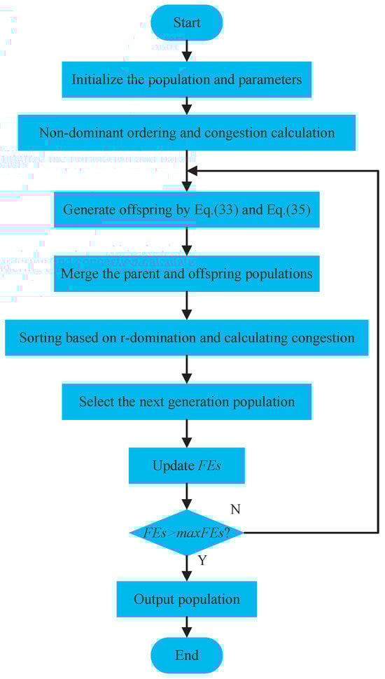
Figure 1. The flowchart of rIMOMFO.

Step 1 Initialization

Initialize the d, n, $max\_FEs$, $FEs$, l, L and $\delta$.

Step 2 Randomly initialize parent population M using Equation (19), and each objective function of every moth is evaluated.

Step 3 Use a non-r-dominated sort method to sort the M and calculate crowding distance [18] for each front.

Step 4 Continue the iterative process or stop.

Run Step 5 to Step 6 until the $FEs$ has reached the $max\_FEs$.

Step 5 The offspring population $M_O$ is generated by the position update mechanism (Equations (33) and (35)) of the IMFO algorithm that is proposed in the previous section.

Step 6 Merge the parent population M and offspring population $M_O$ to create U($U=M\cup M_O$); sort the U and calculate the crowding distance for each front. Then, replace M for the first n members of U.

Step 7 Return the best solutions.

Algorithm 2: rIMOMFO

1: Initialize $max\_FEs$, $n,d$, $FEs=0$, $l=1$, $L=ceil(max\_FEs/(n+7\left)\right)$, $\delta$; 2: Randomly initialize parent population $\mathit{M}$ using Equation (19); 3: Sort the M based on the non-r-dominated sort method, $FEs=FEs+n$; 4: Compute crowding distance [18] for each front; 5: while $FEs\le max\_FEs$ 6:    Generate the offspring population $M_O$ by the position update mechanism (Equations (33) and (35)) of IMFO; 7:    Merge parent population M and offspring population $M_O$ to create U($U=M\cup M_O$); 8:    Sort the U based on the non-r-dominated sort method; 9:    Compute crowding distance for each front; 10:    Replace M for first n members of U; 11:    $l=l+1$; $FEs=FEs+n$; 12: end while 13: return the best solutions

3.4. Computational Complexity of rIMOMFO

The computational complexity of rIMOMFO in one iteration mainly consists of the following two aspects: position update of moths and flames, and non-r-dominated sorting and crowding distance. The complexity order of moth flame position updating is $O\left(n^2\right)$. The computational complexity of non-r-dominated sorting is $O\left(M^{\prime }{n}^2\right)$ ($M^{\prime }$ is the number of objectives); the complexity of crowding distance is $O\left(M^{\prime }logn\right)$. Therefore, the complexity order of rIMOMFO is $O\left(M^{\prime }{n}^2\right)$.

4. Performance Test and Analysis

To verify the effectiveness of rIMOMFO, this section carries out simulation analysis through benchmark test problems. Firstly, benchmark test problems and performance metrics are introduced. Secondly, the test results are given and analyzed.

4.1. Benchmark Test Problems

In this paper, the WFG [55] test problems and 20 test problems [56] in CEC 2009 are used to test the performance of rIMOMFO. WFG is a complex optimization problem, including convexity or concavity and other forms; UF is used for multi-objective unconstrained problems; CF is used for multi-objective constraint problems. In this study, the number of objectives ($M^{\prime }$) is set to 2, 3 (UF,CF) and 4, 7 (WFG), which tests the performance of the algorithm on MOPs and MaOPs, respectively.

4.2. Performance Metrics

In this paper, inverted generational distance (IGD) and hypervolume (HV) are utilized to evaluate UF and CF; generational distance (GD) and spacing (S) are used to evaluate WFG. Their detailed description is as follows:

(1)

Generational distance (GD)

GD is utilized to embody the convergence of a solution set generated by MOAs [57]. A smaller GD value indicates that the convergence of an algorithm is better. If the value of GD is equal to 0, it indicates that all the solutions generated by the algorithm are on the Pareto front. GD is given as

$$\begin{array}{c}\hfill GD\left(A,V\right)={\displaystyle \frac{1}{\left|A\right|}}\sqrt{{\sum }_{M_j\in A}{min}_{M_i\in V}\ast d^{\prime }{\left(M_i,M_j\right)}^2}\end{array}$$

(39)

where $V=\left\{v_1,v_2,\cdots v_n\right\}$ is a set of n targeted points. A is the points of the solution set gained by a specific algorithm. $d^{\prime }\left(M_i,M_j\right)$ indicates the Euclidean distance between $M_i$ and $M_j$.

(2)

Inverted generational distance (IGD)

IGD can simultaneously calculate the convergence and distribution of solutions [58]. The smaller the IGD value, the better the set A. GD is defined as

$$\begin{array}{c}\hfill IGD\left(A,V\right)={\displaystyle \frac{1}{\left|V\right|}}\sum _{i=1}^{\left|V\right|}\underset{M_j\in A}{min}{d}^{\prime }\left(v_i,M_j\right)\end{array}$$

(40)

(3)

Hypervolume (HV)

HV can evaluate the convergence and distribution of the solution set at the same time [59]. A larger HV value indicates that the convergence and distribution of the algorithm is better. HV is given as

$$\begin{array}{c}\hfill HV\left(A,r\right)=volume\left(\underset{f\in A}{\cup }\left[f_1,r_1\right]\times \cdots \left[f_m,r_m\right]\right)\end{array}$$

(41)

where $r={\left(r_1,r_2,\cdots ,r_m\right)}^T$ is a reference point. HV of the A with regard to r is the volume of the region dominated by A and bounded by r [60].

(4)

Spacing (S)

The Spacing metric evaluates the uniformity of the distribution of non-dominated solutions [61]. A smaller S value indicates that the distribution of an algorithm is better. Spacing can be formulated as follows:

$$\begin{array}{c}\hfill S=\sqrt{{\displaystyle \frac{1}{n-1}}\sum _{i=1}^n{\left(\overline{d^{\prime }}-d_i^{\prime }\right)}^2}\end{array}$$

(42)

$$\begin{array}{c}\hfill d_i^{\prime }=\underset{k\ne i}{k\in O}min\sum _{m=1}^{M^{\prime }}\left|O{M}_m^i-O{M}_m^k\right|\end{array}$$

(43)

where $\overline{d^{\prime }}$ is the average of the distances $d_i^{\prime }$ ($i=1,\cdots ,n$). Spacing is the standard deviation of the distance between two continuous solutions of a set O.

4.3. Test Design

To better analyze the performance of rIMOMFO, two groups of comparative tests are utilized. Firstly, based on CF and UF, the proposed rIMOMFO algorithm is compared with other algorithms (NSGAII [18], MAEA [62], MOEAD [19], MOEADDAE [63], CMOPSO [64], dMOPSO [65], MOPSO [66], NSLS [67], NSGAIISDR [68] and NSMFO [69]). Secondly, the rIMOMFO algorithm is tested based on WFG and compared with other algorithms (NSGAII, NSGAIII, MAEA, MOEADDAE, dMOPSO and MOPSO). We reference their original paper for the parameter setting of these comparison algorithms in Table 1. Among them, the selection principle of $\delta =0.1$ refers to the reference literature [51]. $c_{max}=0.9,c_{min}=0.5$. For the test problems of objective function to 2,3,4,7, the population size (n) is set to 100, 100, 286 and 294, respectively. The $maxFEs$ for all test problems is $n\ast 1000$. For WFG test problems, on the basis of [70], the number of position-related variables is $k=18$ and the number of distance-related variables is $l=14$. Additionally, the number of decision variables is set as $d=k+l=32$. In the two groups of comparative tests, each algorithm is run independently 30 times for each problem.

Table 1. Parameter settings.

Algorithm	Parameters
rIMOMFO	$\delta =0.1,t\in [-1,1],b=1,\beta =3/2,c_{max}=0.9,c_{min}=0.5$
NSGAII	$p_c=0.5,p_m=1/D,{\eta }_c={\eta }_m=20$
NSGAIII	$p_c=0.9,p_m=1/D,{\eta }_c={\eta }_m=20$
MAEA	$p_c=1,p_m=1/D,{\eta }_c=30,{\eta }_m=20$
MOEAD	$T=20,p_c=0.5,p_m=1/D,{\eta }_c={\eta }_m=20$
MOEADDAE	$T=20,p_c=0.5,p_m=1/D,{\eta }_c={\eta }_m=20$
CMOPSO	$\gamma =10$
dMOPSO	$T=20,ag{e}_{max}=2$
MOPSO	$T=20,div=10$
NSLS	$T=250,\mu =0.5,\delta =0.1$
NSGAIISDR	$p_c=0.5,p_m=1/D,{\eta }_c={\eta }_m=20$
NSMFO	$t\in [-1,1],b=1,{\eta }_c={\eta }_m=20$

In this paper, five performance evaluation methods are used: Mean, STD, Wilcoxon rank-sum test, multiple-problem Wilcoxon signed-rank test and Friedman rank test. Mean is the average fitness function value of 30 independent runs; STD is the standard deviation of the fitness function value of independent runs; the Wilson rank-sum test is utilized to characterize whether the rIMOMFO is significantly better than other comparative algorithms. In this paper, the significance level of 0.05 is used. “−” means that the rIMOMFO algorithm is better than other algorithms, “+” means that the comparison method is better than rIMOMFO, “=” means that the rIMOMFO and the comparison method are at the same level. In addition, the multiple-problem Wilcoxon signed-rank test is also given for the two groups of simulations. “R+” indicates a positive rank and “R−” indicates a negative rank. “+” and “−” indicate the better than and worse than other algorithms, respectively. At the same time, they indicate that rIMOMFO is different from other algorithms. “=” indicates that the rIMOMFO algorithm is at the same level as the other algorithms and that there is no significant difference. For the Friedman rank test, “Ave” represents the average ranking of the algorithm and “Rank” represents the final ranking of the algorithm. In addition, the bold data in the table represents the results of the optimal algorithm on the corresponding test problem.

4.4. Test Results and Analysis

In this subsection, the WFG and CEC2009 problems are utilized to test the rIMOMFO algorithm, which is compared with the other algorithms. Table 2 and Table 3 show the average and standard deviation for the IGD and HV of 12 algorithms in the CEC2009 test problem, respectively. Table 4, Table 5, Table 6 and Table 7 show the results of the multiple-problem Wilcoxon signed-rank test and Friedman rank test for the IGD and HV of 12 algorithms. The results of nine algorithms on the WFG test are shown in Table 8, Table 9, Table 10, Table 11, Table 12, Table 13, Table 14, Table 15, Table 16, Table 17, Table 18 and Table 19. The tables contain the average, standard deviation, multiple-problem Wilcoxon signed-rank test and Friedman rank test of GD and S of 4 objectives and 7 objectives.

Table 2. Comparison results on IGD value with Mean and STD for CEC 2009.

Problem	${\mathit{M}}^{\prime }$	d	rIMOMFO	NSMFO	NSIMFO	dMOPSO
CF1	2	10	$2.8698\times {10}^{-2}(9.53\times {10}^{-3})$	$6.1278\times {10}^{-2}(7.38\times {10}^{-3})$ −	$5.9692\times {10}^{-2}(8.42\times {10}^{-3})$ −	$3.6101\times {10}^{-1}(1.58\times {10}^{-1})$ −
CF2	2	10	$3.3667\times {10}^{-2}(3.29\times {10}^{-2})$	$7.6282\times {10}^{-2}(1.97\times {10}^{-2})$ −	$7.8324\times {10}^{-2}(1.95\times {10}^{-2})$ −	$9.9901\times {10}^{-2}(1.67\times {10}^{-2})$ −
CF3	2	10	$3.1380\times {10}^{-1}(1.88\times {10}^{-1})$	$3.8902\times {10}^{-1}(9.48\times {10}^{-2})$ =	$4.8233\times {10}^{-1}(1.44\times {10}^{-1})$ −	$8.2756\times {10}^{-1}(9.83\times {10}^{-2})$ −
CF4	2	10	$9.9140\times {10}^{-2}(7.73\times {10}^{-3})$	$\mathbf{9.8520}\times {\mathbf{10}}^{-\mathbf{2}}(\mathbf{7.05}\times {\mathbf{10}}^{-\mathbf{3}})$ =	$1.0051\times {10}^{-1}(9.26\times {10}^{-3})$ =	$2.1646\times {10}^{-1}(4.80\times {10}^{-2})$ −
CF5	2	10	$\mathbf{2.8176}\times {\mathbf{10}}^{-\mathbf{1}}(\mathbf{1.72}\times {\mathbf{10}}^{-\mathbf{1}})$	$6.1082\times {10}^{-1}(6.17\times {10}^{-2})$ −	$6.1481\times {10}^{-1}(4.01\times {10}^{-2})$ −	$6.3177\times {10}^{-1}(1.96\times {10}^{-2})$ −
CF6	2	10	$1.7238\times {10}^{-1}(5.82\times {10}^{-2})$	$1.7774\times {10}^{-1}(3.72\times {10}^{-2})$ =	$1.7150\times {10}^{-1}(3.48\times {10}^{-2})$ =	$1.5528\times {10}^{-1}(4.69\times {10}^{-2})$ =
CF7	2	10	$3.2626\times {10}^{-1}(1.76\times {10}^{-1})$	$3.5408\times {10}^{-1}(1.18\times {10}^{-1})$ =	$3.5139\times {10}^{-1}(1.68\times {10}^{-1})$ =	$1.1040\times {10}^0(2.51\times {10}^{-1})$ −
CF8	3	10	$4.2179\times {10}^{-1}(4.69\times {10}^{-2})$	$5.7041\times {10}^{-1}(1.96\times {10}^{-1})$ −	$5.4272\times {10}^{-1}(1.80\times {10}^{-1})$ −	$3.5161\times {10}^{-1}(4.68\times {10}^{-2})$ +
CF9	3	10	$1.4895\times {10}^{-1}(7.20\times {10}^{-3})$	$2.2420\times {10}^{-1}(3.64\times {10}^{-2})$ −	$2.1492\times {10}^{-1}(3.69\times {10}^{-2})$ −	$1.6574\times {10}^{-1}(1.98\times {10}^{-2})$ −
UF1	2	30	$6.1266\times {10}^{-2}(5.15\times {10}^{-2})$	$1.0692\times {10}^{-1}(1.30\times {10}^{-2})$ −	$1.0315\times {10}^{-1}(1.22\times {10}^{-2})$ =	$3.7787\times {10}^{-1}(8.93\times {10}^{-2})$ −
UF2	2	30	$7.3282\times {10}^{-2}(8.48\times {10}^{-2})$	$7.9242\times {10}^{-2}(8.32\times {10}^{-3})$ −	$8.1809\times {10}^{-2}(8.40\times {10}^{-3})$ −	$9.5804\times {10}^{-2}(1.20\times {10}^{-2})$ −
UF3	2	30	$2.0562\times {10}^{-1}(1.07\times {10}^{-1})$	$2.9676\times {10}^{-1}(1.02\times {10}^{-2})$ −	$2.9996\times {10}^{-1}(9.98\times {10}^{-3})$ −	$3.2026\times {10}^{-1}(8.23\times {10}^{-3})$ −
UF4	2	30	$2.1161\times {10}^{-1}(1.33\times {10}^{-1})$	$8.5698\times {10}^{-2}(2.04\times {10}^{-3})$ =	$8.6195\times {10}^{-2}(2.93\times {10}^{-3})$ =	$1.1669\times {10}^{-1}(4.71\times {10}^{-3})$ =
UF5	2	30	$4.2575\times {10}^{-1}(3.48\times {10}^{-1})$	$7.3601\times {10}^{-1}(7.74\times {10}^{-2})$ −	$7.1110\times {10}^{-1}(1.19\times {10}^{-1})$ −	$2.2858\times {10}^0(3.30\times {10}^{-1})$ −
UF6	2	30	$2.4240\times {10}^{-1}(2.16\times {10}^{-1})$	$4.6809\times {10}^{-1}(1.78\times {10}^{-2})$ −	$4.7172\times {10}^{-1}(1.85\times {10}^{-2})$ −	$1.3868\times {10}^0(4.07\times {10}^{-1})$ −
UF7	2	30	$\mathbf{6.7171}\times {\mathbf{10}}^{-\mathbf{2}}(\mathbf{3.42}\times {\mathbf{10}}^{-\mathbf{2}})$	$8.8191\times {10}^{-2}(5.11\times {10}^{-2})$ =	$8.0029\times {10}^{-2}(7.54\times {10}^{-3})$ =	$2.7840\times {10}^{-1}(7.00\times {10}^{-2})$ −
UF8	3	30	$2.4608\times {10}^{-1}(5.76\times {10}^{-2})$	$2.7633\times {10}^{-1}(8.43\times {10}^{-3})$ −	$2.7919\times {10}^{-1}(1.55\times {10}^{-2})$ −	$3.1537\times {10}^{-1}(2.51\times {10}^{-2})$ −
UF9	3	30	$2.9059\times {10}^{-1}(1.50\times {10}^{-1})$	$\mathbf{2.2564}\times {\mathbf{10}}^{-\mathbf{1}}(\mathbf{1.05}\times {\mathbf{10}}^{-\mathbf{1}})$ =	$2.7597\times {10}^{-1}(1.43\times {10}^{-1})$ =	$6.1699\times {10}^{-1}(4.43\times {10}^{-2})$ −
UF10	3	30	$\mathbf{3.3077}\times {\mathbf{10}}^{-\mathbf{1}}(\mathbf{2.69}\times {\mathbf{10}}^{-\mathbf{2}})$	$3.7228\times {10}^{-1}(5.12\times {10}^{-2})$ −	$3.8012\times {10}^{-1}(6.25\times {10}^{-2})$ −	$9.4592\times {10}^{-1}(7.90\times {10}^{-16})$ −
+/−/=				0/12/7	0/12/7	1/16/2
Problem	${\mathit{M}}^{\prime }$	$\mathit{d}$	NSGAII	MAEA	MOEADDAE	MOPSO
CF1	2	10	$1.9910\times {10}^{-2}(2.53\times {10}^{-3}$) +	$2.0394\times {10}^{-2}(2.00\times {10}^{-3})$ +	$\mathbf{3.3848}\times {\mathbf{10}}^{-\mathbf{3}}(\mathbf{8.78}\times {\mathbf{10}}^{-\mathbf{4}})$ +	$3.8199\times {10}^{-1}(1.47\times {10}^{-1})$ −
CF2	2	10	$4.8788\times {10}^{-2}(1.42\times {10}^{-2})$ −	$5.5329\times {10}^{-2}(2.12\times {10}^{-2})$ −	$7.3556\times {10}^{-2}(4.14\times {10}^{-2})$ −	$1.1013\times {10}^{-1}(4.51\times {10}^{-2})$ −
CF3	2	10	$2.4542\times {10}^{-1}(1.00\times {10}^{-1})$ =	$\mathbf{2.2382}\times {\mathbf{10}}^{-\mathbf{1}}(\mathbf{9.49}\times {\mathbf{10}}^{-\mathbf{2}})$ =	$3.5210\times {10}^{-1}(1.39\times {10}^{-1})$ =	$1.0003\times {10}^0(3.07\times {10}^{-1})$ −
CF4	2	10	$1.1028\times {10}^{-1}(4.61\times {10}^{-2})$ =	$1.0084\times {10}^{-1}(2.79\times {10}^{-2})$ =	$1.9411\times {10}^{-1}(9.40\times {10}^{-2})$ −	$3.6254\times {10}^{-1}(1.56\times {10}^{-1})$ −
CF5	2	10	$3.1665\times {10}^{-1}(1.18\times {10}^{-1})$ =	$2.9797\times {10}^{-1}(1.30\times {10}^{-1})$ =	$3.9289\times {10}^{-1}(1.13\times {10}^{-1})$ −	$1.9165\times {10}^0(1.79\times {10}^0)$ −
CF6	2	10	$1.0287\times {10}^{-1}(3.50\times {10}^{-2})$ +	$\mathbf{8.2431}\times {\mathbf{10}}^{-\mathbf{2}}(\mathbf{3.44}\times {\mathbf{10}}^{-\mathbf{2}})$ +	$8.8390\times {10}^{-2}(5.99\times {10}^{-2})$ +	$1.9473\times {10}^{-1}(7.22\times {10}^{-2})$ =
CF7	2	10	$3.2023\times {10}^{-1}(1.43\times {10}^{-1})$ =	$\mathbf{2.8879}\times {\mathbf{10}}^{-\mathbf{1}}(\mathbf{1.30}\times {\mathbf{10}}^{-\mathbf{1}})$ =	$3.9622\times {10}^{-1}(1.06\times {10}^{-1})$ −	$2.0306\times {10}^0(8.26\times {10}^{-1})$ −
CF8	3	10	$3.8961\times {10}^{-1}(1.18\times {10}^{-1})$ =	$4.0360\times {10}^{-1}(9.13\times {10}^{-2})$ =	$\mathbf{1.9735}\times {\mathbf{10}}^{-\mathbf{1}}(\mathbf{8.38}\times {\mathbf{10}}^{-\mathbf{2}})$ +	$1.5198\times {10}^0(1.84\times {10}^0)$ −
CF9	3	10	$1.6878\times {10}^{-1}(4.14\times {10}^{-2})$ =	$1.3251\times {10}^{-1}(7.75\times {10}^{-2})$ +	$\mathbf{9.4702}\times {\mathbf{10}}^{-\mathbf{2}}(\mathbf{1.24}\times {\mathbf{10}}^{-\mathbf{2}})$ +	$4.8545\times {10}^{-1}(3.57\times {10}^{-1})$ −
UF1	2	30	$1.0514\times {10}^{-1}(3.10\times {10}^{-2})$ =	$1.1171\times {10}^{-1}(3.73\times {10}^{-2})$ −	$1.6842\times {10}^{-1}(9.56\times {10}^{-2})$ −	$5.4448\times {10}^{-1}(1.10\times {10}^{-1})$ −
UF2	2	30	$4.0611\times {10}^{-2}(1.04\times {10}^{-2})$ +	$3.8421\times {10}^{-2}(8.91\times {10}^{-3})$ +	$3.9384\times {10}^{-2}(2.20\times {10}^{-2})$ +	$1.1268\times {10}^{-1}(1.41\times {10}^{-2})$ −
UF3	2	30	$2.2720\times {10}^{-1}(6.51\times {10}^{-2})$ =	$1.9505\times {10}^{-1}(4.26\times {10}^{-2})$ =	$3.2385\times {10}^{-1}(3.42\times {10}^{-2})$ −	$5.4181\times {10}^{-1}(1.98\times {10}^{-2})$ −
UF4	2	30	$4.6471\times {10}^{-2}(1.38\times {10}^{-3})$ +	$4.6193\times {10}^{-2}(2.06\times {10}^{-3})$ +	$5.6695\times {10}^{-2}(5.07\times {10}^{-3})$ +	$1.0149\times {10}^{-1}(1.41\times {10}^{-2})$ =
UF5	2	30	$2.7288\times {10}^{-1}(5.50\times {10}^{-2})$ =	$\mathbf{2.5912}\times {\mathbf{10}}^{-\mathbf{1}}(\mathbf{5.72}\times {\mathbf{10}}^{-\mathbf{2}})$ =	$4.9403\times {10}^{-1}(1.37\times {10}^{-1})$ =	$3.3085\times {10}^0(3.67\times {10}^{-1})$ −
UF6	2	30	$1.8901\times {10}^{-1}(1.06\times {10}^{-1})$ =	$\mathbf{1.7331}\times {\mathbf{10}}^{-\mathbf{1}}(\mathbf{1.07}\times {\mathbf{10}}^{-\mathbf{1}})$ =	$4.6931\times {10}^{-1}(1.97\times {10}^{-1})$ −	$2.5388\times {10}^0(5.97\times {10}^{-1})$ −
UF7	2	30	$1.1900\times {10}^{-1}(1.47\times {10}^{-1})$ =	$1.8747\times {10}^{-1}(1.65\times {10}^{-1})$ =	$4.5141\times {10}^{-1}(2.01\times {10}^{-1})$ −	$6.6410\times {10}^{-1}(1.05\times {10}^{-1})$ −
UF8	3	30	$2.8292\times {10}^{-1}(6.53\times {10}^{-2})$ −	$5.0192\times {10}^{-1}(9.47\times {10}^{-2})$ −	$\mathbf{2.1950}\times {\mathbf{10}}^{-\mathbf{1}}(\mathbf{6.94}\times {\mathbf{10}}^{-\mathbf{2}})$ =	$4.9564\times {10}^{-1}(8.58\times {10}^{-2})$ −
UF9	3	30	$3.4785\times {10}^{-1}(1.02\times {10}^{-1})$ −	$2.6943\times {10}^{-1}(9.97\times {10}^{-2})$ =	$2.5520\times {10}^{-1}(3.99\times {10}^{-2})$ =	$6.2105\times {10}^{-1}(5.43\times {10}^{-2})$ −
UF10	3	30	$4.8468\times {10}^{-1}(8.65\times {10}^{-2})$ −	$4.0996\times {10}^{-1}(8.59\times {10}^{-2})$ −	$4.9002\times {10}^{-1}(9.61\times {10}^{-2})$ −	$2.7099\times {10}^0(3.48\times {10}^{-1})$ −
+/−/=			4/4/11	5/4/10	6/9/4	0/17/2
Problem	${\mathit{M}}^{\prime }$	$\mathit{d}$	MOEAD	CMOPSO	NSLS	NSGAIISDR
CF1	2	10	$6.4319\times {10}^{-1}(0.00\times {10}^0)$ =	$5.8611\times {10}^{-1}(1.72\times {10}^{-1})$ −	$4.7998\times {10}^{-1}(2.16\times {10}^{-1})$ −	$5.4008\times {10}^{-1}(2.87\times {10}^{-1})$ −
CF2	2	10	$2.6824\times {10}^{-1}(1.40\times {10}^{-1})$ −	$\mathbf{1.7403}\times {\mathbf{10}}^{-\mathbf{2}}(\mathbf{3.41}\times {\mathbf{10}}^{-\mathbf{3}})$ =	$1.8924\times {10}^{-1}(4.06\times {10}^{-2})$ −	$4.7097\times {10}^{-2}(1.86\times {10}^{-2})$ −
CF3	2	10	$4.9125\times {10}^{-1}(2.43\times {10}^{-1})$ −	$2.7919\times {10}^{-1}(1.23\times {10}^{-1})$ =	$4.7160\times {10}^0(6.28\times {10}^{-1})$ −	$2.8226\times {10}^{-1}(1.96\times {10}^{-1})$ =
CF4	2	10	$3.5480\times {10}^{-1}(1.29\times {10}^{-1})$ −	$1.9732\times {10}^{-1}(6.45\times {10}^{-2})$ −	$1.8523\times {10}^0(4.17\times {10}^{-1})$ −	$1.9307\times {10}^{-1}(6.68\times {10}^{-2})$ −
CF5	2	10	$4.1160\times {10}^{-1}(1.13\times {10}^{-1})$ −	$3.3186\times {10}^{-1}(1.18\times {10}^{-1})$ −	$8.5467\times {10}^0(1.65\times {10}^0)$ −	$3.0449\times {10}^{-1}(1.29\times {10}^{-1})$ =
CF6	2	10	$2.6255\times {10}^{-1}(6.56\times {10}^{-2})$ −	$1.4362\times {10}^{-1}(5.26\times {10}^{-3})$ =	$3.1328\times {10}^0(1.32\times {10}^0)$ −	$1.2387\times {10}^{-1}(3.45\times {10}^{-2})$ +
CF7	2	10	$4.8383\times {10}^{-1}(1.60\times {10}^{-1})$ −	$3.4670\times {10}^{-1}(9.63\times {10}^{-2})$ =	$8.0252\times {10}^0(1.53\times {10}^0)$ −	$4.1029\times {10}^{-1}(2.75\times {10}^{-1})$ =
CF8	3	10	$3.3785\times {10}^{-1}(1.27\times {10}^{-1})$ +	$2.4942\times {10}^0(9.52\times {10}^{-1})$ −	$5.0857\times {10}^0(2.70\times {10}^0)$ −	$4.1784\times {10}^{-1}(1.40\times {10}^{-1})$ =
CF9	3	10	$2.1135\times {10}^{-1}(2.14\times {10}^{-1})$ =	$5.0082\times {10}^{-1}(1.08\times {10}^{-1})$ −	$7.6614\times {10}^{-1}(1.84\times {10}^{-1})$ −	$1.3755\times {10}^{-1}(5.34\times {10}^{-2})$ +
UF1	2	30	$2.4073\times {10}^{-1}(9.66\times {10}^{-2})$ −	$\mathbf{5.2884}\times {\mathbf{10}}^{-\mathbf{2}}(\mathbf{5.54}\times {\mathbf{10}}^{-\mathbf{3}})$ =	$2.5702\times {10}^{-1}(2.06\times {10}^{-2})$ −	$8.8998\times {10}^{-2}(2.35\times {10}^{-2})$ =
UF2	2	30	$1.6403\times {10}^{-1}(6.15\times {10}^{-2})$ −	$\mathbf{3.0594}\times {\mathbf{10}}^{-\mathbf{2}}(\mathbf{5.43}\times {\mathbf{10}}^{-\mathbf{3}})$ +	$5.5035\times {10}^{-1}(3.38\times {10}^{-2})$ −	$4.4775\times {10}^{-2}(1.40\times {10}^{-2})$ +
UF3	2	30	$3.1533\times {10}^{-1}(2.66\times {10}^{-2})$ −	$\mathbf{1.3684}\times {\mathbf{10}}^{-\mathbf{1}}(\mathbf{4.62}\times {\mathbf{10}}^{-\mathbf{2}})$ =	$3.8707\times {10}^{-1}(4.95\times {10}^{-3})$ −	$2.6673\times {10}^{-1}(5.14\times {10}^{-2})$ =
UF4	2	30	$7.1144\times {10}^{-2}(3.41\times {10}^{-3})$ +	$7.9110\times {10}^{-2}(5.09\times {10}^{-3})$ +	$6.7971\times {10}^{-2}(7.26\times {10}^{-3})$ +	$\mathbf{4.5800}\times {\mathbf{10}}^{-\mathbf{2}}(\mathbf{1.45}\times {\mathbf{10}}^{-\mathbf{3}})$ +
UF5	2	30	$5.3003\times {10}^{-1}(9.88\times {10}^{-2})$ =	$3.6989\times {10}^{-1}(1.14\times {10}^{-1})$ =	$1.9872\times {10}^0(1.21\times {10}^{-1})$ −	$3.0662\times {10}^{-1}(6.86\times {10}^{-2})$ =
UF6	2	30	$4.6892\times {10}^{-1}(1.87\times {10}^{-1})$ −	$2.7849\times {10}^{-1}(1.28\times {10}^{-1})$ =	$1.0974\times {10}^0(5.70\times {10}^{-2})$ −	$1.7719\times {10}^{-1}(1.11\times {10}^{-1})$ =
UF7	2	30	$3.8780\times {10}^{-1}(1.41\times {10}^{-1})$ −	$9.7732\times {10}^{-2}(1.39\times {10}^{-1})$ −	$2.8459\times {10}^{-1}(2.61\times {10}^{-2})$ −	$9.4466\times {10}^{-2}(1.22\times {10}^{-1})$ =
UF8	3	30	$4.0151\times {10}^{-1}(2.63\times {10}^{-1})$ −	$6.8205\times {10}^{-1}(7.99\times {10}^{-2})$ −	$8.0167\times {10}^{-1}(1.08\times {10}^{-1})$ −	$2.2756\times {10}^{-1}(5.91\times {10}^{-2})$ =
UF9	3	30	$3.2670\times {10}^{-1}(3.54\times {10}^{-2})$ =	$9.3291\times {10}^{-1}(1.72\times {10}^{-1})$ −	$1.0171\times {10}^0(1.05\times {10}^{-1})$ −	$3.1514\times {10}^{-1}(7.74\times {10}^{-2})$ =
UF10	3	30	$7.0812\times {10}^{-1}(1.74\times {10}^{-1})$ −	$3.3951\times {10}^0(6.06\times {10}^{-1})$ −	$6.0155\times {10}^0(5.06\times {10}^{-1})$ −	$5.8738\times {10}^{-1}(1.97\times {10}^{-1})$ −
+/−/=			2/13/4	2/9/8	1/18/0	4/4/11

Table 3. Comparison results on HV value with Mean and STD for CEC 2009.

Problem	${\mathit{M}}^{\prime }$	d	rIMOMFO	NSMFO	NSIMFO	dMOPSO
CF1	2	10	$5.3066\times {10}^{-1}(1.13\times {10}^{-2})$	$4.8915\times {10}^{-1}(9.80\times {10}^{-3})$ −	$4.9123\times {10}^{-1}(1.16\times {10}^{-2})$ −	$2.7409\times {10}^{-1}(7.85\times {10}^{-2})$ −
CF2	2	10	$6.3022\times {10}^{-1}(4.83\times {10}^{-2})$	$5.6938\times {10}^{-1}(2.66\times {10}^{-2})$ −	$5.6824\times {10}^{-1}(2.38\times {10}^{-2})$ −	$5.3024\times {10}^{-1}(2.36\times {10}^{-2})$ −
CF3	2	10	$1.2781\times {10}^{-1}(9.56\times {10}^{-2})$	$4.7644\times {10}^{-2}(4.40\times {10}^{-2})$ −	$2.5596\times {10}^{-2}(2.98\times {10}^{-2})$ −	$9.0197\times {10}^{-5}(4.34\times {10}^{-4})$ −
CF4	2	10	$4.0546\times {10}^{-1}(1.06\times {10}^{-2})$	$4.0606\times {10}^{-1}(1.06\times {10}^{-2})$ =	$4.0185\times {10}^{-1}(1.12\times {10}^{-2})$ =	$2.5847\times {10}^{-1}(5.05\times {10}^{-2})$ −
CF5	2	10	$\mathbf{3.1283}\times {\mathbf{10}}^{-\mathbf{1}}(\mathbf{1.10}\times {\mathbf{10}}^{-\mathbf{1}})$	$1.0979\times {10}^{-1}(1.08\times {10}^{-2})$ −	$1.1127\times {10}^{-1}(4.87\times {10}^{-3})$ −	$1.1156\times {10}^{-1}(5.59\times {10}^{-3})$ −
CF6	2	10	$5.5291\times {10}^{-1}(2.77\times {10}^{-2})$	$5.4392\times {10}^{-1}(2.46\times {10}^{-2})$ =	$5.4518\times {10}^{-1}(2.11\times {10}^{-2})$ =	$5.6126\times {10}^{-1}(3.46\times {10}^{-2})$ =
CF7	2	10	$3.8768\times {10}^{-1}(1.19\times {10}^{-1})$	$3.6283\times {10}^{-1}(7.07\times {10}^{-2})$ −	$3.6243\times {10}^{-1}(1.15\times {10}^{-1})$ =	$2.5536\times {10}^{-3}(9.60\times {10}^{-3})$ −
CF8	3	10	$1.0878\times {10}^{-1}(1.80\times {10}^{-2})$	$9.0139\times {10}^{-2}(6.99\times {10}^{-2})$ −	$1.1194\times {10}^{-1}(9.65\times {10}^{-2})$ =	$1.5959\times {10}^{-1}(3.23\times {10}^{-2})$ +
CF9	3	10	$3.0589\times {10}^{-1}(1.06\times {10}^{-2})$	$2.4246\times {10}^{-1}(3.58\times {10}^{-2})$ −	$2.5133\times {10}^{-1}(3.54\times {10}^{-2})$ −	$2.8573\times {10}^{-1}(2.98\times {10}^{-2})$ −
UF1	2	30	$6.3904\times {10}^{-1}(7.33\times {10}^{-2})$	$5.6653\times {10}^{-1}(1.85\times {10}^{-2})$ −	$5.7231\times {10}^{-1}(1.55\times {10}^{-2})$ −	$2.5054\times {10}^{-1}(8.00\times {10}^{-2})$ −
UF2	2	30	$6.4717\times {10}^{-1}(8.26\times {10}^{-2})$	$6.3338\times {10}^{-1}(7.89\times {10}^{-3})$ −	$6.3165\times {10}^{-1}(7.61\times {10}^{-3})$ −	$6.1756\times {10}^{-1}(1.01\times {10}^{-2})$ −
UF3	2	30	$4.5272\times {10}^{-1}(1.31\times {10}^{-1})$	$3.4473\times {10}^{-1}(1.26\times {10}^{-2})$ −	$3.3962\times {10}^{-1}(1.34\times {10}^{-2})$ −	$3.1681\times {10}^{-1}(1.11\times {10}^{-2})$ −
UF4	2	30	$2.6752\times {10}^{-1}(7.18\times {10}^{-2})$	$3.2834\times {10}^{-1}(3.58\times {10}^{-3})$ =	$3.2759\times {10}^{-1}(4.84\times {10}^{-3})$ =	$2.8713\times {10}^{-1}(6.26\times {10}^{-3})$ =
UF5	2	30	$2.2254\times {10}^{-1}(2.27\times {10}^{-1})$	$2.0298\times {10}^{-3}(8.79\times {10}^{-3})$ −	$6.0007\times {10}^{-3}(1.57\times {10}^{-2})$ −	$0.0000\times {10}^0(0.00\times {10}^0)$ −
UF6	2	30	$2.7375\times {10}^{-1}(2.16\times {10}^{-1})$	$4.7045\times {10}^{-2}(6.21\times {10}^{-3})$ −	$4.7490\times {10}^{-2}(5.57\times {10}^{-3})$ −	$0.0000\times {10}^0(0.00\times {10}^0)$ −
UF7	2	30	$\mathbf{4.9503}\times {\mathbf{10}}^{-\mathbf{1}}(\mathbf{4.95}\times {\mathbf{10}}^{-\mathbf{2}})$	$4.6261\times {10}^{-1}(3.56\times {10}^{-2})$ =	$4.6738\times {10}^{-1}(1.02\times {10}^{-2})$ =	$2.3795\times {10}^{-1}(5.98\times {10}^{-2})$ −
UF8	3	30	$\mathbf{3.8152}\times {\mathbf{10}}^{-\mathbf{1}}(\mathbf{6.25}\times {\mathbf{10}}^{-\mathbf{2}})$	$2.9983\times {10}^{-1}(1.01\times {10}^{-2})$ −	$2.9703\times {10}^{-1}(2.36\times {10}^{-2})$ −	$3.0032\times {10}^{-1}(1.51\times {10}^{-2})$ −
UF9	3	30	$4.7033\times {10}^{-1}(1.33\times {10}^{-1})$	$5.3767\times {10}^{-1}(9.42\times {10}^{-2})$ =	$4.9007\times {10}^{-1}(1.27\times {10}^{-1})$ =	$2.0988\times {10}^{-1}(1.89\times {10}^{-2})$ −
UF10	3	30	$\mathbf{2.3217}\times {\mathbf{10}}^{-\mathbf{1}}(\mathbf{2.87}\times {\mathbf{10}}^{-\mathbf{2}})$	$1.9827\times {10}^{-1}(4.63\times {10}^{-2})$ −	$1.9625\times {10}^{-1}(5.04\times {10}^{-2})$ −	$9.0909\times {10}^{-2}(7.06\times {10}^{-17})$ −
+/−/=				0/14/5	0/12/7	1/16/2
Problem	${\mathit{M}}^{\prime }$	$\mathit{d}$	NSGAII	MAEA	MOEADDAE	MOPSO
CF1	2	10	$5.4110\times {10}^{-1}(3.18\times {10}^{-3})$ +	$5.4041\times {10}^{-1}(2.56\times {10}^{-3})$ +	$5.6147\times {10}^{-1}(1.22\times {10}^{-3})$ +	$2.7974\times {10}^{-1}(8.19\times {10}^{-2})$ −
CF2	2	10	$6.0166\times {10}^{-1}(3.04\times {10}^{-2})$ −	$5.9966\times {10}^{-1}(3.49\times {10}^{-2})$ −	$5.8703\times {10}^{-1}(4.33\times {10}^{-2})$ −	$5.1576\times {10}^{-1}(5.18\times {10}^{-2})$ −
CF3	2	10	$1.8536\times {10}^{-1}(4.75\times {10}^{-2})$ +	$1.9644\times {10}^{-1}(4.63\times {10}^{-2})$ +	$1.3338\times {10}^{-1}(3.68\times {10}^{-2})$ =	$5.6964\times {10}^{-3}(1.55\times {10}^{-2})$ −
CF4	2	10	$4.0759\times {10}^{-1}(4.05\times {10}^{-2})$ +	$4.1659\times {10}^{-1}(2.59\times {10}^{-2})$ +	$3.3890\times {10}^{-1}(6.48\times {10}^{-2})$ −	$1.7677\times {10}^{-1}(8.77\times {10}^{-2})$ −
CF5	2	10	$2.7255\times {10}^{-1}(6.21\times {10}^{-2})$ −	$2.8645\times {10}^{-1}(7.19\times {10}^{-2})$ =	$2.1576\times {10}^{-1}(6.35\times {10}^{-2})$ −	$9.4912\times {10}^{-3}(3.32\times {10}^{-2})$ −
CF6	2	10	$6.3293\times {10}^{-1}(1.79\times {10}^{-2})$ +	$6.2457\times {10}^{-1}(2.56\times {10}^{-2})$ +	$6.2118\times {10}^{-1}(7.45\times {10}^{-2})$ +	$4.9723\times {10}^{-1}(6.81\times {10}^{-2})$ −
CF7	2	10	$4.3154\times {10}^{-1}(9.98\times {10}^{-2})$ =	$4.4945\times {10}^{-1}(9.10\times {10}^{-2})$ +	$3.2226\times {10}^{-1}(1.01\times {10}^{-1})$ −	$9.3042\times {10}^{-4}(4.16\times {10}^{-3})$ −
CF8	3	10	$1.8245\times {10}^{-1}(5.10\times {10}^{-2})$ +	$2.0961\times {10}^{-1}(4.10\times {10}^{-2})$ +	$3.7608\times {10}^{-1}(7.33\times {10}^{-2})$ +	$1.0722\times {10}^{-2}(2.76\times {10}^{-2})$ −
CF9	3	10	$3.1707\times {10}^{-1}(5.43\times {10}^{-2})$ +	$3.8859\times {10}^{-1}(5.95\times {10}^{-2})$ +	$4.4702\times {10}^{-1}(2.29\times {10}^{-2})$ +	$1.1062\times {10}^{-1}(9.02\times {10}^{-2})$ −
UF1	2	30	$6.0021\times {10}^{-1}(2.16\times {10}^{-2})$ =	$5.9225\times {10}^{-1}(3.23\times {10}^{-2})$ =	$5.1934\times {10}^{-1}(9.86\times {10}^{-2})$ −	$1.5291\times {10}^{-1}(6.68\times {10}^{-2})$ −
UF2	2	30	$6.7852\times {10}^{-1}(7.31\times {10}^{-3})$ +	$6.7720\times {10}^{-1}(7.62\times {10}^{-3})$ +	$6.8130\times {10}^{-1}(1.20\times {10}^{-2})$ +	$5.9038\times {10}^{-1}(1.39\times {10}^{-2})$ −
UF3	2	30	$4.5576\times {10}^{-1}(5.94\times {10}^{-2})$ =	$4.8397\times {10}^{-1}(3.87\times {10}^{-2})$ =	$3.1779\times {10}^{-1}(4.18\times {10}^{-2})$ −	$1.3405\times {10}^{-1}(1.15\times {10}^{-2})$ −
UF4	2	30	$3.8289\times {10}^{-1}(1.44\times {10}^{-3})$ +	$3.8372\times {10}^{-1}(1.94\times {10}^{-3})$ +	$3.6904\times {10}^{-1}(6.76\times {10}^{-3})$ +	$3.0407\times {10}^{-1}(1.73\times {10}^{-2})$ =
UF5	2	30	$2.1993\times {10}^{-1}(6.14\times {10}^{-2})$ =	$2.5182\times {10}^{-1}(6.12\times {10}^{-2})$ =	$1.6327\times {10}^{-1}(8.96\times {10}^{-2})$ =	$0.0000\times {10}^0(0.00\times {10}^0)$ −
UF6	2	30	$3.0496\times {10}^{-1}(7.28\times {10}^{-2})$ =	$3.3810\times {10}^{-1}(5.72\times {10}^{-2})$ =	$1.5263\times {10}^{-1}(1.00\times {10}^{-1})$ =	$0.0000\times {10}^0(0.00\times {10}^0)$ −
UF7	2	30	$4.7155\times {10}^{-1}(1.02\times {10}^{-1})$ =	$4.2480\times {10}^{-1}(1.17\times {10}^{-1})$ −	$2.4497\times {10}^{-1}(1.31\times {10}^{-1})$ −	$3.3925\times {10}^{-2}(3.36\times {10}^{-2})$ −
UF8	3	30	$2.6374\times {10}^{-1}(5.23\times {10}^{-2})$ −	$3.3744\times {10}^{-1}(1.70\times {10}^{-2})$ =	$3.7411\times {10}^{-1}(4.97\times {10}^{-2})$ =	$1.1239\times {10}^{-1}(4.83\times {10}^{-2})$ −
UF9	3	30	$3.9909\times {10}^{-1}(9.90\times {10}^{-2})$ −	$5.1296\times {10}^{-1}(7.70\times {10}^{-2})$ =	$5.5610\times {10}^{-1}(4.64\times {10}^{-2})$ +	$1.5430\times {10}^{-1}(4.33\times {10}^{-2})$ −
UF10	3	30	$9.0935\times {10}^{-2}(4.21\times {10}^{-2})$ −	$2.0047\times {10}^{-1}(9.17\times {10}^{-2})$ −	$1.2633\times {10}^{-1}(7.65\times {10}^{-2})$ −	$0.0000\times {10}^0(0.00\times {10}^0)$ −
+/−/=			8/5/6	9/3/7	7/8/4	0/18/1
Problem	${\mathit{M}}^{\prime }$	$\mathit{d}$	MOEAD	CMOPSO	NSLS	NSGAIISDR
CF1	2	10	$1.2958\times {10}^{-1}(0.00\times {10}^0)$ =	$1.5349\times {10}^{-1}(8.69\times {10}^{-2})$ −	$1.9053\times {10}^{-1}(9.77\times {10}^{-2})$ −	$1.6299\times {10}^{-1}(1.30\times {10}^{-1})$ −
CF2	2	10	$4.5141\times {10}^{-1}(7.15\times {10}^{-2})$ −	$6.5466\times {10}^{-1}(5.03\times {10}^{-3})$ =	$3.7138\times {10}^{-1}(6.76\times {10}^{-2})$ −	$6.1949\times {10}^{-1}(1.85\times {10}^{-2})$ −
CF3	2	10	$1.0325\times {10}^{-1}(6.09\times {10}^{-2})$ =	$1.4509\times {10}^{-1}(4.37\times {10}^{-2})$ =	$0.0000\times {10}^0(0.00\times {10}^0$ −	$1.5670\times {10}^{-1}(6.72\times {10}^{-2})$ =
CF4	2	10	$2.4000\times {10}^{-1}(8.52\times {10}^{-2})$ −	$3.7293\times {10}^{-1}(4.12\times {10}^{-2})$ −	$6.1138\times {10}^{-4}(3.35\times {10}^{-3})$ −	$3.4538\times {10}^{-1}(4.20\times {10}^{-2})$ −
CF5	2	10	$2.4500\times {10}^{-1}(6.54\times {10}^{-2})$ −	$2.5565\times {10}^{-1}(7.17\times {10}^{-2})$ −	$0.0000\times {10}^0(0.00\times {10}^0)$ −	$2.7266\times {10}^{-1}(6.00\times {10}^{-2})$ −
CF6	2	10	$4.8830\times {10}^{-1}(1.04\times {10}^{-1})$ −	$6.2243\times {10}^{-1}(4.88\times {10}^{-3})$ +	$0.0000\times {10}^0(0.00\times {10}^0)$ −	$6.1437\times {10}^{-1}(1.75\times {10}^{-2})$ +
CF7	2	10	$3.2586\times {10}^{-1}(1.11\times {10}^{-1})$ =	$3.8015\times {10}^{-1}(8.02\times {10}^{-2})$ =	$0.0000\times {10}^0(0.00\times {10}^0)$ −	$3.5335\times {10}^{-1}(1.78\times {10}^{-1})$ =
CF8	3	10	$1.8771\times {10}^{-1}(5.61\times {10}^{-2})$ +	$1.6623\times {10}^{-3}(9.10\times {10}^{-3})$ −	$0.0000\times {10}^0(0.00\times {10}^0)$ −	$1.3176\times {10}^{-1}(5.15\times {10}^{-2})$ =
CF9	3	10	$3.1187\times {10}^{-1}(8.41\times {10}^{-2})$ +	$6.1454\times {10}^{-2}(4.50\times {10}^{-2})$ −	$3.8139\times {10}^{-2}(3.07\times {10}^{-2})$ −	$3.6501\times {10}^{-1}(5.40\times {10}^{-2})$ +
UF1	2	30	$4.8252\times {10}^{-1}(6.33\times {10}^{-2})$ −	$6.4299\times {10}^{-1}(7.79\times {10}^{-3})$ =	$3.5267\times {10}^{-1}(2.66\times {10}^{-2})$ −	$5.9701\times {10}^{-1}(3.26\times {10}^{-2})$ =
UF2	2	30	$6.1762\times {10}^{-1}(3.05\times {10}^{-2})$ −	$6.8643\times {10}^{-1}(5.08\times {10}^{-3})$ +	$9.2689\times {10}^{-2}(2.04\times {10}^{-2})$ −	$6.7308\times {10}^{-1}(6.39\times {10}^{-3})$ +
UF3	2	30	$3.7027\times {10}^{-1}(3.61\times {10}^{-2})$ =	$5.2554\times {10}^{-1}(5.15\times {10}^{-2})$ =	$1.8844\times {10}^{-1}(6.85\times {10}^{-3})$ −	$4.3682\times {10}^{-1}(3.38\times {10}^{-2})$ =
UF4	2	30	$3.3980\times {10}^{-1}(4.76\times {10}^{-3})$ +	$3.3593\times {10}^{-1}(6.68\times {10}^{-3})$ +	$3.5402\times {10}^{-1}(6.39\times {10}^{-3})$ +	$3.8416\times {10}^{-1}(2.26\times {10}^{-3})$ +
UF5	2	30	$1.4183\times {10}^{-1}(7.11\times {10}^{-2})$ =	$2.1658\times {10}^{-1}(7.03\times {10}^{-1})$ =	$0.0000\times {10}^0(0.00\times {10}^0)$ −	$2.1493\times {10}^{-1}(6.21\times {10}^{-2})$ =
UF6	2	30	$2.0221\times {10}^{-1}(8.97\times {10}^{-2})$ =	$2.7339\times {10}^{-1}(7.40\times {10}^{-2})$ =	$0.0000\times {10}^0(0.00\times {10}^0)$ −	$2.9887\times {10}^{-1}(6.15\times {10}^{-2})$ =
UF7	2	30	$2.8245\times {10}^{-1}(9.00\times {10}^{-2})$ −	$4.9245\times {10}^{-1}(1.04\times {10}^{-1})$ −	$1.5377\times {10}^{-1}(4.14\times {10}^{-2})$ −	$4.8750\times {10}^{-1}(8.50\times {10}^{-2})$ =
UF8	3	30	$2.7445\times {10}^{-1}(9.70\times {10}^{-2})$ −	$7.6275\times {10}^{-3}(1.36\times {10}^{-2})$ −	$2.0285\times {10}^{-5}(1.11\times {10}^{-4})$ −	$3.3671\times {10}^{-1}(3.69\times {10}^{-2})$ −
UF9	3	30	$4.4704\times {10}^{-1}(3.09\times {10}^{-2})$ =	$1.4863\times {10}^{-2}(2.33\times {10}^{-2})$ −	$0.0000\times {10}^0(0.00\times {10}^0)$ −	$4.4128\times {10}^{-1}(7.55\times {10}^{-2})$ =
UF10	3	30	$1.1527\times {10}^{-1}(5.93\times {10}^{-2})$ −	$0.0000\times {10}^0(0.00\times {10}^0)$ −	$0.0000\times {10}^0(0.00\times {10}^0$ −	$1.3318\times {10}^{-1}(6.80\times {10}^{-2})$ −
+/−/=			3/9/7	3/9/7	1/18/0	4/6/9

Table 4. Results(IGD) of multiple-problem Wilcoxon signed-rank test.

rIMOMFO VS	R+	R−	p-Value	a = 0.05	rIMOMFO VS	R+	R−	p-Value	a = 0.05
NSIMFO	169	21	0.002902	+	MAEA	72	118	0.354669	=
NSMFO	163	27	0.00621	+	CMOPSO	135	55	0.107466	=
dMOPSO	175	15	0.001285	+	NSGAII	92	98	0.903908	=
MOEADDAE	131	59	0.147416	=	MOPSO	186	4	0.00025	+
MOEAD	178	12	0.000837	+	NSGAIISDR	107	83	0.629162	=
NSLS	189	1	0.000155	+

Table 5. Friedman rank test results(IGD) of the 12 algorithms.

	Rank	Ave		Rank	Ave
rIMOMFO	3	4.11	NSLS	12	10.89
NSIMFO	8	6.32	MAEA	1	3.32
NSMFO	6	6.00	CMOPSO	7	6.11
dMOPSO	10	8.63	NSGAII	2	4.11
MOEADDAE	5	5.05	MOPSO	11	10.58
MOEAD	9	8.42	NSGAIISDR	4	4.47

Table 6. Results(HV) of multiple-problem Wilcoxon signed-rank test.

rIMOMFO VS	R+	R−	p-Value	a = 0.05	rIMOMFO VS	R+	R−	p-Value	a = 0.05
NSIMFO	173	17	0.001696	+	MAEA	53	137	0.090995	=
NSMFO	168	22	0.003307	+	CMOPSO	129	61	0.171239	=
dMOPSO	182	8	0.000463	+	NSGAII	87	103	0.7475	=
MOEADDAE	115	75	0.42091	=	MOPSO	189	1	0.000155	+
MOEAD	170	20	0.002543	+	NSGAIISDR	116	74	0.398063	=
NSLS	189	1	0.000155	+

Table 7. Friedman rank test results(HV) of the 12 algorithms.

	Rank	Ave		Rank	Ave
rIMOMFO	3	4.16	NSLS	12	11.26
NSIMFO	8	6.95	MAEA	1	2.58
NSMFO	7	6.84	CMOPSO	6	5.79
dMOPSO	10	8.95	NSGAII	2	3.74
MOEADDAE	5	5.05	MOPSO	11	10.37
MOEAD	9	7.63	NSGAIISDR	4	4.68

Table 8. Results on GD value with Mean and STD for WFG with 4 objectives.

Problem	${\mathit{M}}^{\prime }$	d	rIMOMFO	NSMFO	NSIMFO
WFG1	4	32	$1.0045\times {10}^{-1}(3.73\times {10}^{-3})$	$9.7284\times {10}^{-2}(6.57\times {10}^{-4})$ +	$9.7192\times {10}^{-2}(4.11\times {10}^{-4})$ +
WFG2	4	32	$2.0881\times {10}^{-2}(2.09\times {10}^{-3})$	$2.2073\times {10}^{-2}(1.34\times {10}^{-3})$ =	$2.1734\times {10}^{-2}(2.14\times {10}^{-3})$ =
WFG3	4	32	$\mathbf{1.3082}\times {\mathbf{10}}^{-\mathbf{2}}(\mathbf{1.74}\times {\mathbf{10}}^{-\mathbf{3}})$	$7.7891\times {10}^{-2}(3.62\times {10}^{-3})$ −	$7.6892\times {10}^{-2}(4.38\times {10}^{-3})$ −
WFG4	4	32	$1.2527\times {10}^{-2}(8.54\times {10}^{-4})$	$3.2630\times {10}^{-2}(2.68\times {10}^{-3})$ −	$3.3885\times {10}^{-2}(3.24\times {10}^{-3})$ −
WFG5	4	32	$1.7769\times {10}^{-2}(4.93\times {10}^{-3})$	$4.5681\times {10}^{-2}(2.84\times {10}^{-3})$ −	$4.5664\times {10}^{-2}(2.54\times {10}^{-3})$ −
WFG6	4	32	$1.6021\times {10}^{-2}(7.94\times {10}^{-4})$	$2.8445\times {10}^{-2}(3.78\times {10}^{-3})$ −	$2.6177\times {10}^{-2}(2.21\times {10}^{-3})$ −
WFG7	4	32	$1.1856\times {10}^{-2}(1.97\times {10}^{-3})$	$4.3988\times {10}^{-2}(4.47\times {10}^{-3})$ −	$4.5818\times {10}^{-2}(5.47\times {10}^{-3})$ −
WFG8	4	32	$\mathbf{2.2620}\times {\mathbf{10}}^{-\mathbf{2}}(\mathbf{3.26}\times {\mathbf{10}}^{-\mathbf{3}})$	$6.1243\times {10}^{-2}(1.96\times {10}^{-3})$ −	$6.0626\times {10}^{-2}(2.29\times {10}^{-3})$ −
WFG9	4	32	$1.2046\times {10}^{-2}(8.35\times {10}^{-4})$	$2.5122\times {10}^{-2}(1.40\times {10}^{-3})$ −	$2.4770\times {10}^{-2}(1.75\times {10}^{-3})$ −
+/−/=			4/4/1	1/7/1	1/7/1
Problem	${\mathit{M}}^{\prime }$	$\mathit{d}$	NSGAII	NSGAIII	MAEA
WFG1	4	32	$7.9191\times {10}^{-3}(7.27\times {10}^{-4})$ +	$2.2631\times {10}^{-2}(5.00\times {10}^{-3})$ +	$2.1797\times {10}^{-2}(5.67\times {10}^{-3})$ +
WFG2	4	32	$4.0024\times {10}^{-2}(4.30\times {10}^{-3})$ −	$8.1623\times {10}^{-3}(1.21\times {10}^{-3})$ +	$8.1614\times {10}^{-3}(1.42\times {10}^{-3})$ +
WFG3	4	32	$1.1431\times {10}^{-1}(2.06\times {10}^{-3})$ −	$1.1438\times {10}^{-1}(6.45\times {10}^{-3})$ −	$1.1353\times {10}^{-1}(1.03\times {10}^{-2})$ −
WFG4	4	32	$1.1611\times {10}^{-2}(6.62\times {10}^{-4})$ +	$8.9768\times {10}^{-3}(3.50\times {10}^{-4})$ +	$8.6626\times {10}^{-3}(1.10\times {10}^{-3})$ +
WFG5	4	32	$1.2070\times {10}^{-2}(6.82\times {10}^{-4})$ +	$1.0104\times {10}^{-2}(1.24\times {10}^{-4})$ +	$1.0156\times {10}^{-2}(1.34\times {10}^{-4})$ +
WFG6	4	32	$1.5919\times {10}^{-2}(1.03\times {10}^{-3})$ =	$1.1682\times {10}^{-2}(7.49\times {10}^{-4})$ +	$1.1785\times {10}^{-2}(6.38\times {10}^{-4})$ +
WFG7	4	32	$9.7505\times {10}^{-3}(3.63\times {10}^{-4})$ +	$7.6139\times {10}^{-3}(2.04\times {10}^{-4})$ +	$7.6124\times {10}^{-3}(1.07\times {10}^{-4})$ +
WFG8	4	32	$5.5758\times {10}^{-2}(1.23\times {10}^{-3})$ −	$3.4975\times {10}^{-2}(6.17\times {10}^{-3})$ −	$3.7177\times {10}^{-2}(7.88\times {10}^{-3})$ −
WFG9	4	32	$1.8052\times {10}^{-2}(5.87\times {10}^{-4})$ −	$1.5477\times {10}^{-2}(2.03\times {10}^{-4})$ −	$1.5425\times {10}^{-2}(4.09\times {10}^{-4})$ −
+/−/=			4/4/1	6/3/0	6/3/0
Problem	${\mathit{M}}^{\prime }$	$\mathit{d}$	MOEADDAE	MOPSO	dMOPSO
WFG1	4	32	$4.3187\times {10}^{-3}(2.03\times {10}^{-4})$ +	$9.6290\times {10}^{-2}(1.42\times {10}^{-3})$ +	$9.3500\times {10}^{-2}(5.71\times {10}^{-4})$ +
WFG2	4	32	$1.6712\times {10}^{-2}(3.09\times {10}^{-3})$ +	$2.1021\times {10}^{-2}(3.18\times {10}^{-3})$ =	$1.7342\times {10}^{-2}(3.25\times {10}^{-3})$ +
WFG3	4	32	$1.1412\times {10}^{-1}(2.88\times {10}^{-3})$ −	$8.7089\times {10}^{-2}(1.03\times {10}^{-2})$ −	$1.0541\times {10}^{-1}(2.42\times {10}^{-3})$ −
WFG4	4	32	$7.6294\times {10}^{-3}(1.66\times {10}^{-4})$ +	$5.1800\times {10}^{-2}(5.40\times {10}^{-3})$ −	$2.6371\times {10}^{-2}(2.06\times {10}^{-3})$ −
WFG5	4	32	$9.2153\times {10}^{-3}(8.21\times {10}^{-5})$ +	$4.7139\times {10}^{-2}(8.24\times {10}^{-3})$ −	$5.2580\times {10}^{-2}(2.79\times {10}^{-3})$ −
WFG6	4	32	$1.0469\times {10}^{-2}(9.90\times {10}^{-4})$ +	$4.0857\times {10}^{-2}(6.45\times {10}^{-3})$ −	$2.1588\times {10}^{-2}(1.87\times {10}^{-3})$ −
WFG7	4	32	$7.7015\times {10}^{-3}(2.09\times {10}^{-4})$ +	$3.8613\times {10}^{-2}(4.31\times {10}^{-3})$ −	$3.7870\times {10}^{-2}(3.75\times {10}^{-3})$ −
WFG8	4	32	$3.0948\times {10}^{-2}(6.01\times {10}^{-3})$ −	$7.1522\times {10}^{-2}(8.64\times {10}^{-3})$ −	$7.1087\times {10}^{-2}(9.64\times {10}^{-3})$ −
WFG9	4	32	$9.7379\times {10}^{-3}(1.76\times {10}^{-3})$ +	$2.4837\times {10}^{-2}(8.27\times {10}^{-3})$ −	$1.9714\times {10}^{-2}(2.03\times {10}^{-3})$ −
+/−/=			7/2/0	1/7/1	2/7/0

Table 9. Results(GD) of multiple-problem Wilcoxon signed-rank test.

rIMOMFO VS	R+	R−	p-Value	a = 0.05	rIMOMFO VS	R+	R−	p-Value	a = 0.05
NSIMFO	43	2	0.015156	+	MAEA	17	28	0.51467	=
NSMFO	43	2	0.015156	+	NSGAIII	16	29	0.441268	=
dMOPSO	41	4	0.028402	+	NSGAII	27	18	0.593955	=
MOEADDAE	15	30	0.374259	=	MOPSO	43	2	0.015156	+

Table 10. Friedman rank test results(GD) of the 9 algorithms.

	Rank	Ave		Rank	Ave
rIMOMFO	4	4.22	MAEA	2	2.89
NSIMFO	7	6.56	NSGAIII	3	3.44
NSMFO	8	7.22	NSGAII	5	5.00
dMOPSO	6	6.11	MOPSO	9	7.33
MOEADDAE	1	2.22

Table 11. Results on S value with Mean and STD for WFG with 4 objectives.

Problem	${\mathit{M}}^{\prime }$	d	rIMOMFO	NSMFO	NSIMFO
WFG1	4	32	$\mathbf{7.6194}\times {\mathbf{10}}^{-\mathbf{2}}(\mathbf{1.86}\times {\mathbf{10}}^{-\mathbf{2}})$	$1.8714\times {10}^{-1}(1.01\times {10}^{-2})$ −	$1.8733\times {10}^{-1}(1.08\times {10}^{-2})$ −
WFG2	4	32	$\mathbf{4.3378}\times {\mathbf{10}}^{-\mathbf{2}}(\mathbf{5.33}\times {\mathbf{10}}^{-\mathbf{3}})$	$1.2370\times {10}^{-1}(1.19\times {10}^{-2})$ −	$1.2235\times {10}^{-1}(8.32\times {10}^{-3})$ −
WFG3	4	32	$\mathbf{3.6044}\times {\mathbf{10}}^{-\mathbf{2}}(\mathbf{1.93}\times {\mathbf{10}}^{-\mathbf{2}})$	$1.9165\times {10}^{-1}(1.09\times {10}^{-2})$ −	$1.9269\times {10}^{-1}(1.01\times {10}^{-2})$ −
WFG4	4	32	$\mathbf{9.5089}\times {\mathbf{10}}^{-\mathbf{2}}(\mathbf{1.01}\times {\mathbf{10}}^{-\mathbf{2}})$	$3.1870\times {10}^{-1}(1.96\times {10}^{-2})$ −	$3.2812\times {10}^{-1}(1.48\times {10}^{-2})$ −
WFG5	4	32	$\mathbf{1.0180}\times {\mathbf{10}}^{-\mathbf{1}}(\mathbf{1.18}\times {\mathbf{10}}^{-\mathbf{2}})$	$2.9353\times {10}^{-1}(1.41\times {10}^{-2})$ −	$2.9164\times {10}^{-1}(1.74\times {10}^{-2})$ −
WFG6	4	32	$\mathbf{1.4668}\times {\mathbf{10}}^{-\mathbf{1}}(\mathbf{2.80}\times {\mathbf{10}}^{-\mathbf{2}})$	$3.2463\times {10}^{-1}(8.14\times {10}^{-3})$ −	$3.2058\times {10}^{-1}(1.54\times {10}^{-2})$ −
WFG7	4	32	$\mathbf{1.0510}\times {\mathbf{10}}^{-\mathbf{1}}(\mathbf{5.76}\times {\mathbf{10}}^{-\mathbf{2}})$	$3.2764\times {10}^{-1}(2.07\times {10}^{-2})$ −	$3.3030\times {10}^{-1}(1.68\times {10}^{-2})$ −
WFG8	4	32	$\mathbf{1.1382}\times {\mathbf{10}}^{-\mathbf{1}}(\mathbf{3.94}\times {\mathbf{10}}^{-\mathbf{2}})$	$2.9270\times {10}^{-1}(2.15\times {10}^{-2})$ −	$2.9421\times {10}^{-1}(2.03\times {10}^{-2})$ −
WFG9	4	32	$\mathbf{1.6369}\times {\mathbf{10}}^{-\mathbf{1}}(\mathbf{2.00}\times {\mathbf{10}}^{-\mathbf{2}})$	$2.9098\times {10}^{-1}(1.18\times {10}^{-2})$ −	$2.9660\times {10}^{-1}(1.63\times {10}^{-2})$ −
+/−/=				0/9/0	0/9/0
Problem	${\mathit{M}}^{\prime }$	$\mathit{d}$	NSGAII	NSGAIII	MAEA
WFG1	4	32	$1.9699\times {10}^{-1}(1.02\times {10}^{-2})$ −	$1.7989\times {10}^{-1}(1.61\times {10}^{-2})$ −	$1.7375\times {10}^{-1}(2.33\times {10}^{-2})$ −
WFG2	4	32	$2.0424\times {10}^{-1}(2.00\times {10}^{-2})$ −	$1.6191\times {10}^{-1}(1.56\times {10}^{-2})$ −	$1.6619\times {10}^{-1}(2.28\times {10}^{-2})$ −
WFG3	4	32	$2.3996\times {10}^{-1}(1.02\times {10}^{-2})$ −	$2.0896\times {10}^{-1}(1.38\times {10}^{-2})$ −	$2.0889\times {10}^{-1}(2.34\times {10}^{-2})$ −
WFG4	4	32	$3.2545\times {10}^{-1}(1.39\times {10}^{-2})$ −	$3.2219\times {10}^{-1}(8.44\times {10}^{-3})$ −	$3.1101\times {10}^{-1}(3.42\times {10}^{-2})$ −
WFG5	4	32	$3.2423\times {10}^{-1}(1.37\times {10}^{-2})$ −	$3.0373\times {10}^{-1}(9.93\times {10}^{-3})$ −	$3.0331\times {10}^{-1}(7.59\times {10}^{-3})$ −
WFG6	4	32	$3.2252\times {10}^{-1}(1.56\times {10}^{-2})$ −	$3.2651\times {10}^{-1}(1.39\times {10}^{-2})$ −	$3.1932\times {10}^{-1}(1.03\times {10}^{-2})$ −
WFG7	4	32	$3.3006\times {10}^{-1}(1.53\times {10}^{-2})$ −	$3.2220\times {10}^{-1}(5.68\times {10}^{-3})$ −	$3.2062\times {10}^{-1}(6.37\times {10}^{-3})$ −
WFG8	4	32	$3.3971\times {10}^{-1}(1.93\times {10}^{-2})$ −	$3.7674\times {10}^{-1}(3.84\times {10}^{-2})$ −	$3.7697\times {10}^{-1}(2.50\times {10}^{-2})$ −
WFG9	4	32	$2.9382\times {10}^{-1}(1.28\times {10}^{-2})$ −	$3.1515\times {10}^{-1}(1.50\times {10}^{-2})$ −	$3.0612\times {10}^{-1}(7.77\times {10}^{-3})$ −
+/−/=			0/9/0	0/9/0	0/9/0
Problem	${\mathit{M}}^{\prime }$	$\mathit{d}$	MOEADDAE	MOPSO	dMOPSO
WFG1	4	32	$9.2582\times {10}^{-2}(1.09\times {10}^{-2})$ −	$1.7391\times {10}^{-1}(1.96\times {10}^{-2})$ −	$1.3444\times {10}^{-1}(1.13\times {10}^{-2})$ −
WFG2	4	32	$1.5010\times {10}^{-1}(1.33\times {10}^{-2})$ −	$1.2475\times {10}^{-1}(3.69\times {10}^{-2})$ −	$1.4682\times {10}^{-1}(2.13\times {10}^{-2})$ −
WFG3	4	32	$1.1342\times {10}^{-1}(9.17\times {10}^{-3})$ −	$1.2274\times {10}^{-1}(1.84\times {10}^{-2})$ −	$2.1809\times {10}^{-1}(7.69\times {10}^{-3})$ −
WFG4	4	32	$2.1818\times {10}^{-1}(1.09\times {10}^{-2})$ −	$1.7802\times {10}^{-1}(2.64\times {10}^{-2})$ −	$4.9739\times {10}^{-1}(1.98\times {10}^{-2})$ −
WFG5	4	32	$2.1679\times {10}^{-1}(6.91\times {10}^{-3})$ −	$1.7532\times {10}^{-1}(2.48\times {10}^{-2})$ −	$4.8868\times {10}^{-1}(1.80\times {10}^{-2})$ −
WFG6	4	32	$2.0012\times {10}^{-1}(1.47\times {10}^{-2})$ −	$2.0522\times {10}^{-1}(3.26\times {10}^{-2})$ −	$5.1778\times {10}^{-1}(2.41\times {10}^{-2})$ −
WFG7	4	32	$2.1410\times {10}^{-1}(8.12\times {10}^{-3})$ −	$2.2726\times {10}^{-1}(4.03\times {10}^{-2})$ −	$4.9350\times {10}^{-1}(3.60\times {10}^{-2})$ −
WFG8	4	32	$2.1258\times {10}^{-1}(1.59\times {10}^{-2})$ −	$2.6279\times {10}^{-1}(1.87\times {10}^{-2})$ −	$7.0593\times {10}^{-1}(5.20\times {10}^{-2})$ −
WFG9	4	32	$1.8671\times {10}^{-1}(1.28\times {10}^{-2})$ −	$1.6613\times {10}^{-1}(2.90\times {10}^{-2})$ =	$5.4398\times {10}^{-1}(1.17\times {10}^{-2})$ −
+/−/=			0/9/0	0/8/1	0/9/0

Table 12. Results(S) of multiple-problem Wilcoxon signed-rank test.

rIMOMFO VS	R+	R−	p-Value	a = 0.05	rIMOMFO VS	R+	R−	p-Value	a = 0.05
NSIMFO	45	0	0.007686	+	MAEA	45	0	0.007686	+
NSMFO	45	0	0.007686	+	NSGAIII	45	0	0.007686	+
dMOPSO	45	0	0.007686	+	NSGAII	45	0	0.007686	+
MOEADDAE	45	0	0.007686	+	MOPSO	45	0	0.007686	+

Table 13. Friedman rank test results(S) of the 9 algorithms.

	Rank	Ave		Rank	Ave
rIMOMFO	1	1.00	MAEA	5	5.67
NSIMFO	6	5.67	NSGAIII	7	6.78
NSMFO	4	5.00	NSGAII	8	7.33
dMOPSO	9	7.78	MOPSO	3	3.00
MOEADDAE	2	2.78

Table 14. Results on GD value with Mean and STD for WFG with 7 objectives.

Problem	${\mathit{M}}^{\prime }$	d	rIMOMFO	NSMFO	NSIMFO
WFG1	7	32	$1.2578\times {10}^{-1}(1.50\times {10}^{-3})$	$1.3619\times {10}^{-1}(5.99\times {10}^{-4})$ −	$1.3621\times {10}^{-1}(4.58\times {10}^{-4})$ −
WFG2	7	32	$4.2745\times {10}^{-2}(1.69\times {10}^{-3})$	$5.8522\times {10}^{-2}(4.77\times {10}^{-3})$ −	$5.6744\times {10}^{-2}(5.39\times {10}^{-3})$ −
WFG3	7	32	$\mathbf{4.8731}\times {\mathbf{10}}^{-\mathbf{2}}(\mathbf{1.66}\times {\mathbf{10}}^{-\mathbf{3}})$	$2.0498\times {10}^{-1}(6.91\times {10}^{-3})$ −	$2.0911\times {10}^{-1}(9.85\times {10}^{-3})$ −
WFG4	7	32	$7.6228\times {10}^{-2}(1.95\times {10}^{-3})$	$1.1656\times {10}^{-1}(1.05\times {10}^{-3})$ −	$1.1656\times {10}^{-1}(1.05\times {10}^{-3})$ −
WFG5	7	32	$9.4960\times {10}^{-2}(6.56\times {10}^{-3})$	$1.1937\times {10}^{-1}(1.30\times {10}^{-3})$ −	$1.1900\times {10}^{-1}(1.39\times {10}^{-3})$ −
WFG6	7	32	$8.4997\times {10}^{-2}(3.90\times {10}^{-3})$	$1.1452\times {10}^{-1}(1.67\times {10}^{-3})$ −	$1.1373\times {10}^{-1}(2.45\times {10}^{-3})$ −
WFG7	7	32	$1.5085\times {10}^{-1}(7.49\times {10}^{-2})$	$1.2521\times {10}^{-1}(3.71\times {10}^{-3})$ =	$1.2378\times {10}^{-1}(3.75\times {10}^{-3})$ =
WFG8	7	32	$7.7985\times {10}^{-2}(6.40\times {10}^{-3})$	$1.3261\times {10}^{-1}(1.89\times {10}^{-3})$ −	$1.3256\times {10}^{-1}(1.34\times {10}^{-3})$ −
WFG9	7	32	$\mathbf{7.1724}\times {\mathbf{10}}^{-\mathbf{2}}(\mathbf{2.64}\times {\mathbf{10}}^{-\mathbf{3}})$	$1.2114\times {10}^{-1}(9.10\times {10}^{-4})$ −	$1.2194\times {10}^{-1}(1.16\times {10}^{-3})$ −
+/−/=				0/8/1	0/8/1
Problem	${\mathit{M}}^{\prime }$	$\mathit{d}$	NSGAII	NSGAIII	MAEA
WFG1	7	32	$3.2363\times {10}^{-2}(1.13\times {10}^{-3})$ +	$2.3080\times {10}^{-2}(3.93\times {10}^{-3})$ +	$2.5076\times {10}^{-2}(3.48\times {10}^{-3})$ +
WFG2	7	32	$1.1224\times {10}^{-1}(6.43\times {10}^{-3})$ −	$2.4157\times {10}^{-2}(6.14\times {10}^{-3})$ +	$2.6029\times {10}^{-2}(4.40\times {10}^{-3})$ +
WFG3	7	32	$2.9305\times {10}^{-1}(5.10\times {10}^{-3})$ −	$1.7635\times {10}^{-1}(9.94\times {10}^{-2})$ −	$1.6234\times {10}^{-1}(8.43\times {10}^{-2})$ −
WFG4	7	32	$1.0516\times {10}^{-1}(2.88\times {10}^{-3})$ −	$6.0744\times {10}^{-2}(1.16\times {10}^{-3})$ +	$5.8597\times {10}^{-2}(2.53\times {10}^{-3})$ +
WFG5	7	32	$1.0568\times {10}^{-1}(2.22\times {10}^{-3})$ −	$5.9792\times {10}^{-2}(1.60\times {10}^{-3})$ +	$6.0789\times {10}^{-2}(8.44\times {10}^{-4})$ +
WFG6	7	32	$1.0500\times {10}^{-1}(3.42\times {10}^{-3})$ −	$6.1967\times {10}^{-2}(5.96\times {10}^{-4})$ +	$6.2134\times {10}^{-2}(8.04\times {10}^{-4})$ +
WFG7	7	32	$1.0168\times {10}^{-1}(3.72\times {10}^{-3})$ =	$5.3740\times {10}^{-2}(2.52\times {10}^{-3})$ +	$5.6887\times {10}^{-2}(4.28\times {10}^{-3})$ +
WFG8	7	32	$1.2400\times {10}^{-1}(1.88\times {10}^{-3})$ −	$7.6764\times {10}^{-2}(7.44\times {10}^{-3})$ =	$8.1558\times {10}^{-2}(4.37\times {10}^{-3})$ =
WFG9	7	32	$1.2018\times {10}^{-1}(3.13\times {10}^{-3})$ −	$8.1048\times {10}^{-2}(3.76\times {10}^{-3})$ −	$8.3187\times {10}^{-2}(1.44\times {10}^{-3})$ −
+/−/=			1/7/1	6/2/1	6/2/1
Problem	${\mathit{M}}^{\prime }$	$\mathit{d}$	MOEADDAE	MOPSO	dMOPSO
WFG1	7	32	$1.8661\times {10}^{-2}(2.60\times {10}^{-3})$ +	$1.3392\times {10}^{-1}(1.39\times {10}^{-3})$ −	$1.2780\times {10}^{-1}(2.20\times {10}^{-3})$ −
WFG2	7	32	$3.1607\times {10}^{-2}(3.59\times {10}^{-3})$ +	$5.4369\times {10}^{-2}(1.37\times {10}^{-2})$ −	$2.0863\times {10}^{-2}(6.72\times {10}^{-3})$ +
WFG3	7	32	$2.4959\times {10}^{-1}(4.60\times {10}^{-3})$ −	$1.9219\times {10}^{-1}(3.34\times {10}^{-2})$ −	$2.5034\times {10}^{-1}(2.65\times {10}^{-3})$ −
WFG4	7	32	$6.3606\times {10}^{-2}(2.07\times {10}^{-3})$ +	$8.6604\times {10}^{-2}(2.11\times {10}^{-2})$ =	$9.2928\times {10}^{-2}(1.27\times {10}^{-2})$ −
WFG5	7	32	$6.3665\times {10}^{-2}(1.43\times {10}^{-3})$ +	$1.2554\times {10}^{-1}(5.65\times {10}^{-3})$ −	$1.2663\times {10}^{-1}(3.19\times {10}^{-3})$ −
WFG6	7	32	$6.8164\times {10}^{-2}(4.76\times {10}^{-3})$ +	$1.2120\times {10}^{-1}(1.13\times {10}^{-2})$ −	$8.1963\times {10}^{-2}(2.11\times {10}^{-2})$ =
WFG7	7	32	$6.5593\times {10}^{-2}(2.46\times {10}^{-3})$ +	$8.8933\times {10}^{-2}(1.63\times {10}^{-2})$ =	$2.0194\times {10}^{-1}(2.86\times {10}^{-2})$ =
WFG8	7	32	$1.0980\times {10}^{-1}(7.90\times {10}^{-3})$ −	$1.0693\times {10}^{-1}(1.15\times {10}^{-2})$ −	$1.7196\times {10}^{-1}(4.35\times {10}^{-2})$ −
WFG9	7	32	$8.2895\times {10}^{-2}(3.57\times {10}^{-3})$ −	$8.6247\times {10}^{-2}(8.76\times {10}^{-3})$ −	$1.0157\times {10}^{-1}(5.86\times {10}^{-3})$ −
+/−/=			6/3/0	0/7/2	1/6/2

Table 15. Results(GD) of multiple-problem Wilcoxon signed-rank test.

rIMOMFO VS	R+	R−	p-Value	a = 0.05	rIMOMFO VS	R+	R−	p-Value	a = 0.05
NSIMFO	41	4	0.028402	+	MAEA	12	33	0.213524	=
NSMFO	41	4	0.028402	+	NSGAIII	11	34	0.173071	=
dMOPSO	39	6	0.050612	=	NSGAII	31	14	0.313938	=
MOEADDAE	17	28	0.51467	=	MOPSO	37	8	0.085831	=

Table 16. Friedman rank test results(gd) of the 9 algorithms.

	Rank	Ave		Rank	Ave
rIMOMFO	4	3.89	MAEA	2	2.44
NSIMFO	8	7.33	NSGAIII	1	1.67
NSMFO	9	7.44	NSGAII	6	6.44
dMOPSO	7	6.44	MOPSO	5	5.78
MOEADDAE	3	3.56

Table 17. Results on S value with Mean and STD for WFG with 7 objectives.

Problem	${\mathit{M}}^{\prime }$	d	rIMOMFO	NSMFO	NSIMFO
WFG1	7	32	$\mathbf{2.5062}\times {\mathbf{10}}^{-\mathbf{1}}(\mathbf{4.15}\times {\mathbf{10}}^{-\mathbf{2}})$	$5.2863\times {10}^{-1}(2.46\times {10}^{-2})$ −	$5.2911\times {10}^{-1}(2.58\times {10}^{-2})$ −
WFG2	7	32	$\mathbf{6.8079}\times {\mathbf{10}}^{-\mathbf{2}}(\mathbf{8.04}\times {\mathbf{10}}^{-\mathbf{3}})$	$4.3550\times {10}^{-1}(1.90\times {10}^{-2})$ −	$4.5184\times {10}^{-1}(4.07\times {10}^{-2})$ −
WFG3	7	32	$\mathbf{1.1753}\times {\mathbf{10}}^{-\mathbf{1}}(\mathbf{2.22}\times {\mathbf{10}}^{-\mathbf{2}})$	$6.0935\times {10}^{-1}(2.20\times {10}^{-2})$ −	$6.1981\times {10}^{-1}(3.95\times {10}^{-2})$ −
WFG4	7	32	$2.7994\times {10}^{-1}(2.83\times {10}^{-2})$	$1.1865\times {10}^0(5.10\times {10}^{-2})$ −	$1.1865\times {10}^0(5.10\times {10}^{-2})$ −
WFG5	7	32	$\mathbf{3.8156}\times {\mathbf{10}}^{-\mathbf{1}}(\mathbf{6.10}\times {\mathbf{10}}^{-\mathbf{2}})$	$1.1308\times {10}^0(5.47\times {10}^{-2})$ −	$1.1603\times {10}^0(6.17\times {10}^{-2})$ −
WFG6	7	32	$5.6354\times {10}^{-1}(1.50\times {10}^{-1})$	$1.1864\times {10}^0(4.60\times {10}^{-2})$ −	$1.1940\times {10}^0(5.27\times {10}^{-2})$ −
WFG7	7	32	$5.1728\times {10}^{-1}(3.64\times {10}^{-1})$	$1.1503\times {10}^0(6.18\times {10}^{-2})$ −	$1.1439\times {10}^0(5.89\times {10}^{-2})$ −
WFG8	7	32	$9.2131\times {10}^{-1}(3.40\times {10}^{-1})$	$1.1414\times {10}^0(6.20\times {10}^{-2})$ −	$1.1279\times {10}^0(5.50\times {10}^{-2})$ −
WFG9	7	32	$9.4718\times {10}^{-1}(1.62\times {10}^{-1})$	$1.2353\times {10}^0(4.73\times {10}^{-2})$ −	$1.2431\times {10}^0(7.70\times {10}^{-2})$ −
+/−/=				0/9/0	0/9/0
Problem	${\mathit{M}}^{\prime }$	$\mathit{d}$	NSGAII	NSGAIII	MAEA
WFG1	7	32	$5.8495\times {10}^{-1}(2.61\times {10}^{-2})$ −	$5.6928\times {10}^{-1}(1.06\times {10}^{-1})$ −	$6.2071\times {10}^{-1}(1.32\times {10}^{-1})$ −
WFG2	7	32	$8.5097\times {10}^{-1}(2.94\times {10}^{-2})$ −	$5.2450\times {10}^{-1}(1.71\times {10}^{-1})$ −	$4.9411\times {10}^{-1}(1.47\times {10}^{-1})$ −
WFG3	7	32	$9.1848\times {10}^{-1}(4.74\times {10}^{-2})$ −	$6.0914\times {10}^{-1}(1.23\times {10}^{-1})$ −	$6.2036\times {10}^{-1}(1.46\times {10}^{-1})$ −
WFG4	7	32	$1.4044\times {10}^0(3.30\times {10}^{-2})$ −	$1.1872\times {10}^0(1.76\times {10}^{-2})$ −	$1.2648\times {10}^0(1.28\times {10}^{-1})$ −
WFG5	7	32	$1.4482\times {10}^0(4.42\times {10}^{-2})$ −	$9.8470\times {10}^{-1}(2.97\times {10}^{-2})$ −	$9.9299\times {10}^{-1}(1.63\times {10}^{-2})$ −
WFG6	7	32	$1.4467\times {10}^0(8.22\times {10}^{-2})$ −	$1.0099\times {10}^0(1.31\times {10}^{-2})$ −	$1.0010\times {10}^0(2.05\times {10}^{-2})$ −
WFG7	7	32	$1.4814\times {10}^0(4.38\times {10}^{-2})$ −	$1.2221\times {10}^0(9.76\times {10}^{-2})$ −	$1.1407\times {10}^0(1.00\times {10}^{-1})$ −
WFG8	7	32	$1.4507\times {10}^0(5.35\times {10}^{-2})$ −	$1.4201\times {10}^0(1.21\times {10}^{-1})$ −	$1.4514\times {10}^0(5.62\times {10}^{-2})$ −
WFG9	7	32	$1.3474\times {10}^0(7.76\times {10}^{-2})$ −	$1.2557\times {10}^0(9.28\times {10}^{-2})$ −	$1.2022\times {10}^0(7.95\times {10}^{-2})$ −
+/−/=			0/9/0	0/9/0	0/9/0
Problem	${\mathit{M}}^{\prime }$	$\mathit{d}$	MOEADDAE	MOPSO	dMOPSO
WFG1	7	32	$3.0931\times {10}^{-1}(8.46\times {10}^{-2})$ =	$5.6116\times {10}^{-1}(5.20\times {10}^{-2})$ −	$2.9765\times {10}^{-1}(1.33\times {10}^{-2})$ −
WFG2	7	32	$3.9510\times {10}^{-1}(8.92\times {10}^{-2})$ −	$1.3538\times {10}^{-1}(7.11\times {10}^{-2})$ −	$2.0257\times {10}^{-1}(3.96\times {10}^{-2})$ −
WFG3	7	32	$5.8096\times {10}^{-1}(4.65\times {10}^{-2})$ −	$1.6674\times {10}^{-1}(6.27\times {10}^{-2})$ −	$9.0846\times {10}^{-1}(4.87\times {10}^{-2})$ −
WFG4	7	32	$8.6219\times {10}^{-1}(5.99\times {10}^{-2})$ −	$8.9371\times {10}^{-2}(5.55\times {10}^{-2})$ +	$1.6015\times {10}^0(1.28\times {10}^{-1})$ −
WFG5	7	32	$9.3242\times {10}^{-1}(3.57\times {10}^{-2})$ −	$5.8306\times {10}^{-1}(9.11\times {10}^{-2})$ −	$1.8775\times {10}^0(5.63\times {10}^{-2})$ −
WFG6	7	32	$8.1869\times {10}^{-1}(6.53\times {10}^{-2})$ −	$3.1169\times {10}^{-1}(1.22\times {10}^{-1})$ +	$1.7599\times {10}^0(1.70\times {10}^{-1})$ −
WFG7	7	32	$8.2562\times {10}^{-1}(3.93\times {10}^{-2})$ −	$2.4024\times {10}^{-1}(8.13\times {10}^{-2})$ =	$1.8017\times {10}^0(3.40\times {10}^{-1})$ −
WFG8	7	32	$8.7501\times {10}^{-1}(7.86\times {10}^{-2})$ +	$3.0871\times {10}^{-1}(6.59\times {10}^{-2})$ +	$1.1285\times {10}^0(3.74\times {10}^{-1})$ =
WFG9	7	32	$7.8691\times {10}^{-1}(5.12\times {10}^{-2})$ +	$4.6196\times {10}^{-1}(1.05\times {10}^{-1})$ +	$1.6503\times {10}^0(1.90\times {10}^{-1})$ −
+/−/=			2/6/1	4/4/1	0/8/1

Table 18. Results(S) of multiple-problem Wilcoxon signed-rank test.

rIMOMFO VS	R+	R−	p-Value	a = 0.05	rIMOMFO VS	R+	R−	p-Value	a = 0.05
NSIMFO	45	0	0.007686	+	MAEA	45	0	0.007686	+
NSMFO	45	0	0.007686	+	NSGAIII	45	0	0.007686	+
dMOPSO	45	0	0.007686	+	NSGAII	45	0	0.007686	+
MOEADDAE	41	4	0.028402	+	MOPSO	14	31	0.313938	=

Table 19. Friedman rank test results(S) of the 9 algorithms.

	Rank	Ave		Rank	Ave
rIMOMFO	1	1.78	MAEA	7	6.22
NSIMFO	5	5.67	NSGAIII	6	6.11
NSMFO	4	5.22	NSGAII	9	8.22
dMOPSO	8	7.00	MOPSO	2	1.89
MOEADDAE	3	2.89

In Table 2, rIMOMFO is better than the other 11 algorithms in CF5, UF7 and UF10, and it has the same level as the other algorithms in the other test problems. NSMFO and NSIMFO are inferior to rIMOMFO in 12 test problems and have the same performance in 7 test problems. IMFO has the same or better performance than MFO in most test problems, which shows that the improvement of IMFO is very effective. It can be seen intuitively in Table 5 that the ranking of rIMOMFO is 3; the average ranking is 4.11. MAEA and NSGAII are the first and second, and the ranking of the other nine algorithms is behind rIMOMFO. At the same time, it can be seen in Table 4 that although MAEA and NSGAII are better than rIMOMFO, there is no significant difference between them and rIMOMFO. In Table 5, rIMOMFO is superior to the other 11 algorithms in CF5, UF7, UF8 and UF10. The overall performance of NSGAII and MOEAD in CEC 2009 is better than that of rIMOMFO, but they have similar convergence and distribution in most test problems. In Table 7, the ranking of rIMOMFO is 3, with an average ranking of 4.16. For the first- and second-ranked MAEA and NSGAII, it can be seen in Table 6 that there is no significant difference between them and rIMOMFO.

In Table 8, rIMOMFO is superior to the other 11 algorithms in WFG3 and WFG8. And it also shows good competitiveness in other test problems. It can be seen intuitively in Table 10 that the ranking of rIMOMFO is 4; the average ranking is 4.22. MOEADDAE, MAEA and NSGAII are the first, second and third, and the other five algorithms are ranked behind rIMOMFO. At the same time, Table 9 shows that although MOEADDAE, MAEA and NSGAIII are better than rIMOMFO, there is no significant difference between them and rIMOMFO. In addition, rIMOMFO shows good performance on all problems except WFG9 in Table 11. In Table 13, the ranking of rIMOMFO is 1, with an average ranking of 1.00. From Table 12, there is a significant difference between rIMOMFO and the other algorithms. For the WFG problems with 7 objectives, Table 14 and Table 17 show that the results of rIMOMFO are also competitive. It can be seen intuitively in Table 16 that the ranking of rIMOMFO is 4; the average ranking is 4.22. NSGAIII, MAEA and MOEADDAE are the first, second and third, and the ranking of the other five algorithms is behind rIMOMFO. At the same time, it can be seen in Table 15 that although NSGAIII, MAEA and MOEADDAE are better than rIMOMFO, there is no significant difference between them and rIMOMFO. In addition, in Table 19, the ranking of rIMOMFO is 1, with an average ranking of 1.78. From Table 18, there is a significant difference between rIMOMFO and the other algorithms.

Therefore, through the above tests, it can be concluded that the proposed rIMOMFO method is competitive with the other 12 methods in terms of search performance.

4.5. Ablation Experiments

To verify the effectiveness of each module of the algorithm proposed in this article, ablation experiments were conducted. Table 20 presents the experimental results, indicating the algorithm names corresponding to each improved mechanism. Among them, ✓ indicates the adoption of corresponding strategies, while × indicates the non adoption of corresponding strategies. From the table, it can be seen that rIMOMFO has better convergence and diversity than rIMOMFO-DHI, rIMOMFO-DH and rIMOMFO-I.

Table 20. Comparative results for ablation experiments.

Algorithm	Dynamic Adjustment Mechanism	Hybrid Mutation Strategy	Improved Moth Position Update	IGD +/−/≈	HV +/−/≈
rIMOMFO-DHI vs. rIMOMFO	×	×	×	0/27/1	0/26/2
rIMOMFO-DI vs. rIMOMFO	×	✓	×	1/22/5	1/21/6
rIMOMFO-I vs. rIMOMFO	✓	✓	×	5/18/5	5/17/6

5. Application of rIMOMFO for Parameter Optimization of a Multiple Spacecraft Attitude Controller

In this section, the rIMOMFO algorithm is utilized to solve the MOP of the parameter optimization of a multiple spacecraft attitude controller. Firstly, spacecraft parameters are given. Then, the effectiveness of the rIMOMFO algorithm is verified. Finally, the attitude coordinative control performance of the multiple spacecraft controller is obtained based on the optimized parameters.

5.1. Simulation Conditions

The interaction between different spacecraft is symmetrical, and the simulation topology presented in this paper is also symmetrical. In this paper, a multiple spacecraft model with one virtual leader and four followers is adopted. Figure 2 [71] shows the communication topology of the multiple spacecraft model.

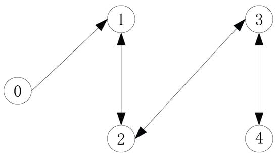
Figure 2. Communication topology of multiple spacecraft model.

The inertial matrices of the four followers are $J_1=diag\left\{17,12,9\right\}$, $J_2=diag\left\{14,13,10\right\}$, $J_3=diag\left\{20,10,12\right\}$ and $J_4=diag\left\{15,9,16\right\}$. The virtual leader’s posture is $q_0={\left[0.5,0,0\right]}^T$. The external interference of the system is ${\epsilon }_i=0.1\ast {\left[cos\left(0.2t\right),sin\left(0.3t\right),cos\left(0.4t\right)\right]}^T$ N·m. The efficiency factor of the actuator fault is ${\Xi }_i=diag\left\{0.2,0.4,1\right\}$. The deviation fault is ${\mathit{f}}_{ai}=\left[{\mathit{f}}_{ai1},\right.{\mathit{f}}_{ai2},{\left.{\mathit{f}}_{ai3}\right]}^T$, ${\mathit{f}}_{ai1}=0.05\ast \left(0.9+0.1\ast sin\left(t/10\right)+0.01\ast \varpi \right)$ N·m, ${\mathit{f}}_{ai2}=0.05\ast \left(0.9+0.1\ast cos\left(t/10\right)+0.015\ast \varpi \right)$ N·m, ${\mathit{f}}_{ai3}=0.05\ast \left(0.9+0.1\ast sin\left(t/10\right)+0.02\ast \varpi \right)$ N·m; $\varpi \in \left[-1,1\right]$ is random number. The parameters of the adaptive sliding mode interference observer are $r_i=0.05$, ${\gamma }_i=0.5$, ${\eta }_i=0.1$ and ${\mathsf{\ell }}_{i,1}=0.2$.

If parameter optimization is not used to determine the controller parameters of multiple spacecraft, the parameters need to be determined through the controller design process and experience. This method requires substantial knowledge of controller design and multiple spacecraft systems and takes a lot of time. In this paper, four algorithms (rIMOMFO, rNSMFO, NSIMFO and NSMFO) are utilized to solve the MOP of a multiple spacecraft system. rNSMFO, NSIMFO and NSMFO are the most similar algorithms to rIMOMFO, which can further illustrate the effectiveness of rIMOMFO in practical applications. The population size is 40 and the $maxFEs$ is 4000. The other parameters of these algorithms are given in the previous section.

5.2. Results and Analysis

The root mean square error between 10 s and 15 s is used to reflect the stability of attitude tracking; 10 s is a hypothetical threshold of the maximum adjust time to reach stability. Figure 3 shows that all the solutions generated by rIMOMFO are lower than the threshold. The other three methods are not be stable within 8 s. This means that it is difficult for them to solve the multiple spacecraft optimization problem in a given evaluation range. Therefore, the proposed rIMOMFO algorithm has the ability to solve the multiple spacecraft optimization problem.

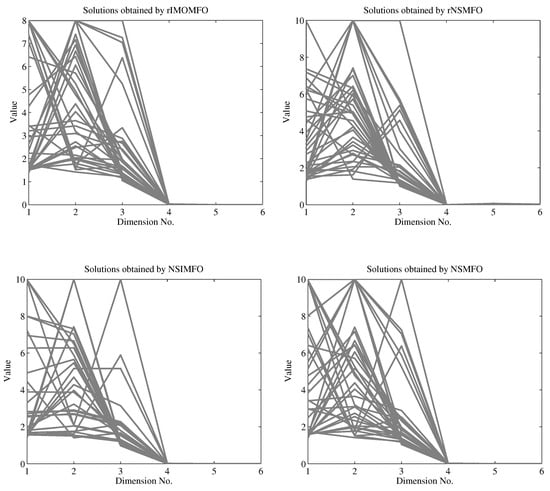
Figure 3. Solutions obtained by rIMOMFO, rNSMFO, NSIMFO and NSMFO.

This section gives the running results of these four algorithms, and the selected solutions are given in Table 21 and Table 22. According to these solutions, the performance of the attitude coordinative control of multiple spacecraft is shown in Figure 4, Figure 5, Figure 6 and Figure 7.

Table 21. Solutions from rIMOMFO, rNSMFO, NSIMFO and NSMFO.

Algorithms	${\mathit{\delta }}_{11}$	${\mathit{\delta }}_{21}$	${\mathit{\delta }}_{31}$	${\mathit{\delta }}_{41}$	${\mathit{\delta }}_{12}$	${\mathit{\delta }}_{22}$	${\mathit{\delta }}_{32}$	${\mathit{\delta }}_{42}$	${\mathit{\mu }}_{11}$
rNSMFO	0.947	0.296	0.006	0.044	0.090	0.317	0.182	0.009	0.482
NSMFO	0.037	0.588	0.383	0.884	1.115	1.119	0.136	0.105	0.297
NSIMFO	1.296	0.350	0.161	0.842	0.981	0.030	0.049	0.159	0.145
rIMOMFO	0.640	0.296	0.000	0.767	0.265	0.330	0.212	0.139	0.094
Algorithms	${\mathit{\mu }}_{\mathbf{21}}$	${\mathit{\mu }}_{\mathbf{31}}$	${\mathit{\mu }}_{\mathbf{41}}$	${\mathit{\mu }}_{\mathbf{12}}$	${\mathit{\mu }}_{\mathbf{22}}$	${\mathit{\mu }}_{\mathbf{32}}$	${\mathit{\mu }}_{\mathbf{42}}$	${\mathit{\beta }}_{\mathbf{2}}$
rNSMFO	0.575	0.028	1.182	0.052	0.653	0.224	0.246	0.428
NSMFO	0.166	0.344	0.190	0.552	0.296	0.034	0.493	0.191
NSIMFO	0.258	0.315	0.080	0.063	0.373	0.169	0.022	0.485
rIMOMFO	0.150	0.207	0.189	0.310	0.466	0.185	0.566	0.544

Table 22. Objectives value of the corresponding solution.

Algorithms	${\mathit{f}}_1$	${\mathit{f}}_2$	${\mathit{f}}_3$	${\mathit{f}}_4$	${\mathit{f}}_5$	${\mathit{f}}_6$
rNSMFO	2.2	4.22	1.31	$6.13\times {10}^5$	$1.74\times {10}^5$	$3.17\times {10}^5$
NSMFO	1.73	1.42	1.22	$4.71\times {10}^4$	$4.52\times {10}^4$	$5.22\times {10}^4$
NSIMFO	2.82	2.85	2.21	$1.16\times {10}^5$	$7.19\times {10}^5$	$1.85\times {10}^5$
rIMOMFO	3.2	3.42	2.67	$\mathbf{5.98}\times {\mathbf{10}}^{\mathbf{6}}$	$\mathbf{6.06}\times {\mathbf{10}}^{\mathbf{6}}$	$\mathbf{2.24}\times {\mathbf{10}}^{\mathbf{6}}$

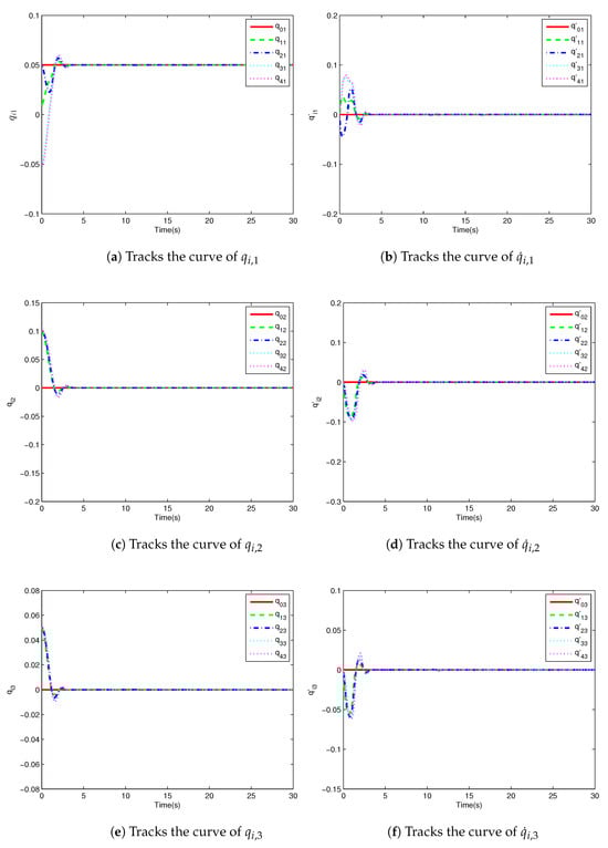
Figure 4. Multiple spacecraft attitudes and their derivative tracking curves with rIMOMFO.

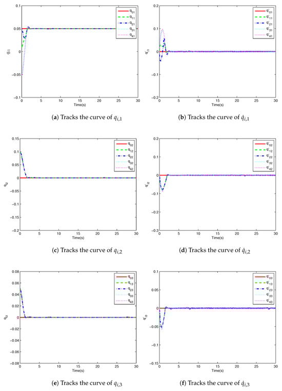
Figure 5. Multiple spacecraft attitudes and their derivative tracking curves with rNSMFO.

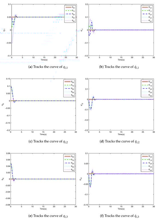
Figure 6. Multiple spacecraft attitudes and their derivative tracking curves with NSIMFO.

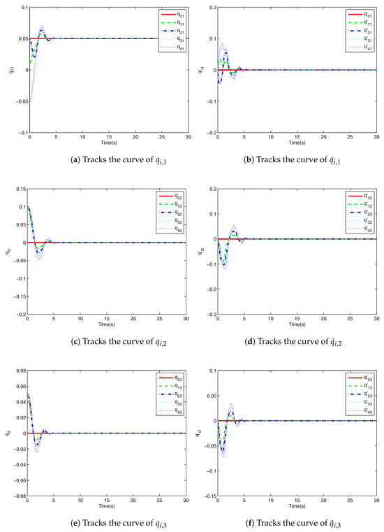
Figure 7. Multiple spacecraft attitudes and their derivative tracking curves with NSMFO.

Figure 3 shows the attitude tracking curve based on rIMOMFO. $q_{i,j}$ and ${\dot{q}}_{i,j}$ are the j-th attitude and its derivatives of the i-th spacecraft. Figure 4 shows three states of the four spacecraft attitudes and their derivatives. Accordingly, the attitude tracking curves based on rNSMFO, NSIMFO and NSMFO are shown in Figure 5, Figure 6 and Figure 7, respectively. It can be seen from the figures that the attitudes of multiple spacecraft can converge to a stable state. In addition, Table 22 shows that the tracking accuracy of the rIMOMFO-optimized controller can reach ${10}^{-6}$, which is better than that for the other three algorithms. In addition, the adjustment time is longer. However, for the whole control process, the adjustment time of rIMOMFO is acceptable. Therefore, controllers optimized by rIMOMFO can obtain higher control accuracies with acceptable adjustment times.

6. Conclusions and Future Work

In this paper, the MOP of parameter optimization for a multiple spacecraft attitude controller is established, and an improved multi-objective moth–flame optimization algorithm based on r-dominant sorting (rIMOMFO) is proposed. In rIMOMFO, the Cauchy mutation is utilized to produce flames that lead moths to updated positions to improve the search performance of MFO. Secondly, a hybrid mutation operator is utilized to perturb the positions of the moths. Among them, the variation in the numbers of flames and moths can be dynamically adjusted by calculating the difference of fitness variance between the two generations of moths. In addition, an adaptive parameter is applied to the moth position update mechanism to further balance the exploitation and exploration. Finally, r-domination is used to guide the search toward the preference of the decision maker. Based on the WFG and CEC2009 test problems, rIMOMFO is compared with 12 other MOEAs, and the results show that the rIMOMFO algorithm is feasible and effective. Furthermore, rIMOMFO is used to optimize the parameters of an attitude cooperative controller for multiple spacecraft, and the results show that the optimized controller can improve the control accuracy and accelerate the convergence speed. Therefore, the rIMOMFO algorithm proposed in this paper can be utilized to solve MOPs in practical engineering.

In further research work, the improvement of MFO performance and the domination relationship with a stronger distribution can be studied. Simultaneously, the proposed rIMOMFO can be applied to practical devices, considering issues such as communication delay, actuator saturation and scalability for larger formations.

References

- Wu, B.; Xu, C.; Zhang, Y. Decentralized adaptive control for attitude synchronization of multiple spacecraft via quantized information exchange. Acta Astronaut. 2020, 175, 57–65. [Google Scholar] [CrossRef]
- Ren, W.; Beard, R. A decentralized scheme for spacecraft formation flying via the virtual structure approach. In Proceedings of the 2003 American Control Conference, Denver, CO, USA, 4–6 June 2003; Volume 2, pp. 1746–1751. [Google Scholar]
- Du, H.; Li, S.; Qian, C. Finite-Time Attitude Tracking Control of Spacecraft With Application to Attitude Synchronization. IEEE Trans. Autom. Control 2011, 56, 2711–2717. [Google Scholar] [CrossRef]
- Liu, X.; Kumar, K.D. Network-Based Tracking Control of Spacecraft Formation Flying with Communication Delays. IEEE Trans. Aerosp. Electron. Syst. 2012, 48, 2302–2314. [Google Scholar] [CrossRef]
- Xu, M.; Fang, Y.; Li, J.; Zhao, X. Attitude coordinated output feedback control based on event triggering for multiple spacecrafts. Int. J. Control 2022, 95, 2438–2447. [Google Scholar] [CrossRef]
- Hu, Q.; Zhang, J.; Zhang, Y. Velocity-free attitude coordinated tracking control for spacecraft formation flying. ISA Trans. 2018, 73, 54–65. [Google Scholar] [CrossRef]
- Zou, A.M.; de Ruiter,, A.H.; Kumar, K.D. Distributed finite-time velocity-free attitude coordination control for spacecraft formations. Automatica 2016, 67, 46–53. [Google Scholar] [CrossRef]
- Hu, Q.; Shi, Y.; Wang, C. Event-Based Formation Coordinated Control for Multiple Spacecraft Under Communication Constraints. IEEE Trans. Syst. Man Cybern. Syst. 2021, 51, 3168–3179. [Google Scholar] [CrossRef]
- Tan, L.; Luo, J.; Liu, J.; Zhang, S. Cooperative autonomous obstacle avoidance control of spacecraft cluster via event-triggered reference governors. J. Frankl. Inst. 2024, 361, 107027. [Google Scholar] [CrossRef]
- Tang, Y.; Lai, B.; Li, X.; Zou, A.M.; Yang, X. Distributed finite-time attitude coordination control of spacecraft formations with multiple constraints. Int. J. Robust Nonlinear Control 2024, 34, 15. [Google Scholar] [CrossRef]
- Li, L.; Du, L.; Hu, Y. Cooperative control method of multiple spacecraft formation based on graphtheory. J. Comput. Methods Sci. Eng. 2024, 24, 1237–1251. [Google Scholar] [CrossRef]
- Yang, X.; Chen, Q.; Xie, S.; He, X. Adaptive Predefined-Time Event-Triggered Control for Attitude Consensus of Multiple Spacecraft With Time-Varying State Constraints. IEEE Trans. Syst. Man, Cybern. Syst. 2025, 55, 3756–3768. [Google Scholar] [CrossRef]
- Gong, Z.; Liu, C.; Teo, K.L.; Wu, Y. A gradient-based optimization algorithm to solve optimal control problems with conformable fractional-order derivatives. J. Comput. Appl. Math. 2025, 454, 116169. [Google Scholar] [CrossRef]
- Naifar, O. Tempered fractional gradient descent: Theory, algorithms, and robust learning applications. Neural Netw. 2026, 193, 108005. [Google Scholar]
- Chen, K.; Luo, W.; Zhou, Q.; Liu, Y.; Xu, P.; Shi, Y. A Novel Immune Algorithm for Multiparty Multiobjective Optimization. IEEE Trans. Emerg. Top. Comput. Intell. 2025, 9, 1238–1252. [Google Scholar] [CrossRef]
- Tanabe, R.; Ishibuchi, H. A Review of Evolutionary Multimodal Multiobjective Optimization. IEEE Trans. Evol. Comput. 2020, 24, 193–200. [Google Scholar] [CrossRef]
- Moldovan, D.; Slowik, A. Energy consumption prediction of appliances using machine learning and multi-objective binary grey wolf optimization for feature selection. Appl. Soft Comput. 2021, 111, 107745. [Google Scholar] [CrossRef]
- Deb, K.; Pratap, A.; Agarwal, S.; Meyarivan, T. A fast and elitist multiobjective genetic algorithm: NSGA-II. IEEE Trans. Evol. Comput. 2002, 6, 182–197. [Google Scholar] [CrossRef]
- Zhang, Q.; Li, H. MOEA/D: A Multiobjective Evolutionary Algorithm Based on Decomposition. IEEE Trans. Evol. Comput. 2007, 11, 712–731. [Google Scholar] [CrossRef]
- Kim, M.; Hiroyasu, T.; Miki, M.; Watanabe, S. SPEA2+: Improving the Performance of the Strength Pareto Evolutionary Algorithm 2. In Proceedings of the International Conference on Parallel Problem Solving from Nature, Birmingham, UK, 18–22 September 2004; pp. 742–751. [Google Scholar]
- Deb, K.; Jain, H. An Evolutionary Many-Objective Optimization Algorithm Using Reference-Point-Based Nondominated Sorting Approach, Part I: Solving Problems With Box Constraints. IEEE Trans. Evol. Comput. 2014, 18, 577–601. [Google Scholar] [CrossRef]
- Cui, Z.; Wu, Y.; Zhao, T.; Zhang, W.; Chen, J. A two-stage accelerated search strategy for large-scale multi-objective evolutionary algorithm. Inf. Sci. 2025, 686, 121347. [Google Scholar] [CrossRef]
- Qiao, K.; Yu, K.; Yue, C.; Qu, B.; Liu, M.; Liang, J. A Cooperative Multistep Mutation Strategy for Multiobjective Optimization Problems With Deceptive Constraints. IEEE Trans. Syst. Man, Cybern. Syst. 2024, 54, 6670–6682. [Google Scholar] [CrossRef]
- Ma, J.; Zhang, Y.; Wang, Y.; Gong, D.; Sun, X.; Zeng, B. A Multitask Multiobjective Operation Optimization Method for Coal Mine Integrated Energy System. IEEE Trans. Ind. Inform. 2024, 20, 11149–11160. [Google Scholar] [CrossRef]
- Chen, K.; Luo, W.; Lin, X.; Song, Z.; Chang, Y. Evolutionary Biparty Multiobjective UAV Path Planning: Problems and Empirical Comparisons. IEEE Trans. Emerg. Top. Comput. Intell. 2024, 8, 2433–2445. [Google Scholar] [CrossRef]
- Li, Z.; Luo, C.; Parr, G.; Min, G. Optimization for Control and Data Traffic in Aerial–Terrestrial AxV Networks: A Multiobjective Policy-Based Learning Approach. IEEE Internet Things J. 2025, 12, 33026–33040. [Google Scholar] [CrossRef]
- Pham, T.H. On efficient solutions of nonsmooth fractional multiobjective optimization problems with mixed constraints. Appl. Anal. 2025, 1–34. [Google Scholar] [CrossRef]
- Coello, C.; Pulido, G.; Lechuga, M. Handling multiple objectives with particle swarm optimization. IEEE Trans. Evol. Comput. 2004, 8, 256–279. [Google Scholar] [CrossRef]
- Konak, A.; Coit, D.W.; Smith, A.E. Multi-objective optimization using genetic algorithms: A tutorial. Reliab. Eng. Syst. Saf. 2006, 91, 992–1007. [Google Scholar] [CrossRef]
- Das, S.; Suganthan, P.N. Differential Evolution: A Survey of the State-of-the-Art. IEEE Trans. Evol. Comput. 2011, 15, 4–31. [Google Scholar] [CrossRef]
- Pierezan, J.; Dos Santos Coelho, L. Coyote Optimization Algorithm: A New Metaheuristic for Global Optimization Problems. In Proceedings of the 2018 IEEE Congress on Evolutionary Computation (CEC), Rio de Janeiro, Brazil, 8–13 July 2018; pp. 1–8. [Google Scholar]
- Yuan, X.; Zhu, Z.; Yang, Z.; Zhang, Y. MSCSO: A Modified Sand Cat Swarm Optimization for Global Optimization and Multilevel Thresholding Image Segmentation. Symmetry 2025, 17, 2012. [Google Scholar] [CrossRef]
- Yang, X.S. Firefly Algorithm. Eng. Optim. Introd. Metaheuristic Appl. 2010, 9, 221–230. [Google Scholar]
- Faramarzi, A.; Heidarinejad, M.; Stephens, B.; Mirjalili, S. Equilibrium optimizer: A novel optimization algorithm. Knowl.-Based Syst. 2020, 191, 105190. [Google Scholar] [CrossRef]
- Ginidi, A.R.; Elsayed, A.M.; Shaheen, A.M.; Elattar, E.E.; El-Sehiemy, R.A. A Novel Heap-Based Optimizer for Scheduling of Large-Scale Combined Heat and Power Economic Dispatch. IEEE Access 2021, 9, 83695–83708. [Google Scholar] [CrossRef]
- Gandomi, A.; Yang, X.; Alavi, A. Cuckoo search algorithm: A metaheuristic approach to solve structural optimization problems. Eng. Comput. 2013, 29, 17–35. [Google Scholar] [CrossRef]
- Mirjalili, S. SCA: A Sine Cosine Algorithm for solving optimization problems. Knowl.-Based Syst. 2016, 96, 120–133. [Google Scholar] [CrossRef]
- Sharma, V.; Pattnaik, S.S.; Garg, T. A review of bacterial foraging optimization and its applications. Procedia-Soc. Behav. Sci. 2012, 48, 1294–1303. [Google Scholar]
- Sulaiman, M.H.; Mustaffa, Z.; Saari, M.M.; Daniyal, H.; Daud, M.R.; Razali, S.; Mohamed, A.I. Barnacles Mating Optimizer: A Bio-Inspired Algorithm for Solving Optimization Problems. In Proceedings of the 2018 19th IEEE/ACIS International Conference on Software Engineering, Artificial Intelligence, Networking and Parallel/Distributed Computing (SNPD), Busan, Republic of Korea, 27–29 June 2018; pp. 265–270. [Google Scholar] [CrossRef]
- Mirjalili, S. Moth-flame optimization algorithm: A novel nature-inspired heuristic paradigm. Knowl.-Based Syst. 2015, 89, 228–249. [Google Scholar] [CrossRef]
- Liang, S.; Liu, Z.; You, D.; Pan, W.; Zhao, J.; Cao, Y. PSO-NRS: An online group feature selection algorithm based on PSO multi-objective optimization. Appl. Intell. 2023, 53, 15095–15111. [Google Scholar] [CrossRef]
- Ghasemi, M.; Bagherifard, K.; Parvin, H.; Nejatian, S.; Pho, K.H. Multi-objective whale optimization algorithm and multi-objective grey wolf optimizer for solving next release problem with developing fairness and uncertainty quality indicators. Appl. Intell. 2021, 51, 5358–5387. [Google Scholar] [CrossRef]
- Mirjalili, S.; Saremi, S.; Mirjalili, S.M.; dos S. Coelho, L. Multi-objective grey wolf optimizer: A novel algorithm for multi-criterion optimization. Expert Syst. Appl. 2016, 47, 106–119. [Google Scholar] [CrossRef]
- Balasubbareddy, M.; Sivanagaraju, S.; Suresh, C.V. Multi-objective optimization in the presence of practical constraints using non-dominated sorting hybrid cuckoo search algorithm. Eng. Sci. Technol. Int. J. 2015, 18, 603–615. [Google Scholar] [CrossRef]
- Zhai, Y.K.; Xu, Y.; Gan, J.Y. A novel artificial fish swarm algorithm based on multi-objective optimization. In Proceedings of the International Conference on Intelligent Computing, Huangshan, China, 25–29 July 2012; Volume 7390, pp. 67–73. [Google Scholar]
- Hassanien, A.E.; Gaber, T.; Mokhtar, U.; Hefny, H. An improved moth flame optimization algorithm based on rough sets for tomato diseases detection. Comput. Electron. Agric. 2017, 136, 86–96. [Google Scholar] [CrossRef]
- Shehab, M.; Abualigah, L.; Hamad, H.A.; Alabool, H.; Alshinwan, M.; Khasawneh, A.M. Moth-flame optimization algorithm: Variants and applications. Neural Comput. Appl. 2020, 32, 9859–9884. [Google Scholar] [CrossRef]
- Chung, S.J.; Ahsun, U.; Slotine, J. Application of Synchronization to Formation Flying Spacecraft: Lagrangian Approach. J. Guid. Control Dyn. 2008, 32, 512–526. [Google Scholar] [CrossRef]
- Xu, M.; Fang, Y.; Li, J.; Zhao, X. Finite time distributed coordinated control for attitude of multi-spacecraft based on super-twisting algorithm. Control Theory Appl. 2021, 38, 924–932. [Google Scholar]
- Zhao, X.; Fang, Y.; Ma, S.; Liu, Z. Multi-swarm improved moth-flame optimization algorithm with chaotic grouping and Gaussian mutation for solving engineering optimization problems. Expert Syst. Appl. 2022, 204, 117562. [Google Scholar] [CrossRef]
- Ben Said, L.; Bechikh, S.; Ghedira, K. The r-Dominance: A New Dominance Relation for Interactive Evolutionary Multicriteria Decision Making. IEEE Trans. Evol. Comput. 2010, 14, 801–818. [Google Scholar] [CrossRef]
- Yu, X.; Cai, M.; Cao, J. A novel mutation differential evolution for global optimization. J. Intell. Fuzzy Syst. 2015, 28, 1047–1060. [Google Scholar] [CrossRef]
- Wang, G.G.; Deb, S.; Gandomi, A.H.; Alavi, A.H. Opposition-based krill herd algorithm with Cauchy mutation and position clamping. Neurocomputing 2016, 177, 147–157. [Google Scholar] [CrossRef]
- Luo, J.; Chen, H.; Zhang, Q.; Xu, Y.; Huang, H.; Zhao, X. An improved grasshopper optimization algorithm with application to financial stress prediction. Appl. Math. Model. 2018, 64, 654–668. [Google Scholar] [CrossRef]
- Huband, S.; Hingston, P.; Barone, L.; While, L. A review of multiobjective test problems and a scalable test problem toolkit. IEEE Trans. Evol. Comput. 2006, 10, 477–506. [Google Scholar] [CrossRef]
- Zhang, Q.; Zhou, A.; Zhao, S.Z.; Suganthan, P.N.; Liu, W.; Tiwari, S. Multiobjective optimization Test Instances for the CEC 2009 Special Session and Competition. Mech. Eng. 2008, 264, 1–30. [Google Scholar]
- Hu, J.; Yu, G.; Zheng, J.; Zou, J. A preference-based multi-objective evolutionary algorithm using preference selection radius. Soft Comput. 2017, 21, 5025–5051. [Google Scholar] [CrossRef]
- Zitzler, E.; Thiele, L.; Laumanns, M.; Fonseca, C.; da Fonseca, V. Performance assessment of multiobjective optimizers: An analysis and review. IEEE Trans. Evol. Comput. 2003, 7, 117–132. [Google Scholar] [CrossRef]
- Zitzler, E.; Thiele, L. Multiobjective evolutionary algorithms: A comparative case study and the strength Pareto approach. IEEE Trans. Evol. Comput. 1999, 3, 257–271. [Google Scholar] [CrossRef]
- Zhang, Z.; Qin, H.; Yao, L.; Liu, Y.; Jiang, Z.; Feng, Z.; Ouyang, S. Improved Multi-objective Moth-flame Optimization Algorithm based on R-domination for cascade reservoirs operation. J. Hydrol. 2020, 581, 124431. [Google Scholar] [CrossRef]
- Schott, J. Fault Tolerant Design Using Single and Multicriteria Genetic Algorithm Optimization. Master’s Thesis, Massachusetts Institute of Technology, Cambridge, MA, USA, 1995. [Google Scholar]
- Xiong, Z.; Yang, J.; Zhao, Z.; Wang, Y.; Yang, Z. Maximum angle evolutionary selection for many-objective optimization algorithm with adaptive reference vector. J. Intell. Manuf. 2023, 34, 961–984. [Google Scholar] [CrossRef]
- Zhu, Q.; Zhang, Q.; Lin, Q. A Constrained Multiobjective Evolutionary Algorithm With Detect-and-Escape Strategy. IEEE Trans. Evol. Comput. 2020, 24, 938–947. [Google Scholar] [CrossRef]
- Zhang, X.; Zheng, X.; Cheng, R.; Qiu, J.; Jin, Y. A competitive mechanism based multi-objective particle swarm optimizer with fast convergence. Inf. Sci. 2018, 427, 63–76. [Google Scholar] [CrossRef]
- Zapotecas Martínez, S.; Coello Coello, C.A. A Multi-Objective Particle Swarm Optimizer Based on Decomposition. Assoc. Comput. Mach. GECCO ’11 2011, 8, 69–76. [Google Scholar]
- Coello Coello, C.; Lechuga, M. MOPSO: A Proposal for Multiple Objective Particle Swarm. In Proceedings of the 2002 Congress on Evolutionary Computation, CEC’02, Honolulu, HI, USA, 12–17 May 2002; Volume 2, pp. 1051–1056. [Google Scholar]
- Chen, B.; Zeng, W.; Lin, Y.; Zhang, D. A New Local Search-Based Multiobjective Optimization Algorithm. IEEE Trans. Evol. Comput. 2015, 19, 50–73. [Google Scholar] [CrossRef]
- Tian, Y.; Cheng, R.; Zhang, X.; Su, Y.; Jin, Y. A Strengthened Dominance Relation Considering Convergence and Diversity for Evolutionary Many-Objective Optimization. IEEE Trans. Evol. Comput. 2019, 23, 331–345. [Google Scholar] [CrossRef]
- Savsani, V.; Tawhid, M.A. Non-dominated sorting moth flame optimization (NS-MFO) for multi-objective problems. Eng. Appl. Artif. Intell. 2017, 63, 20–32. [Google Scholar] [CrossRef]
- Wang, R.; Purshouse, R.C.; Fleming, P.J. Preference-inspired co-evolutionary algorithms using weight vectors. Eur. J. Oper. Res. 2015, 243, 423–441. [Google Scholar] [CrossRef]
- Xu, M.; Fang, Y.; Li, J.; Zhao, X. Finite Time Fully Distributed Consensus Control for Multi-agent System With Input Saturation and Limited Communication Resources. Int. J. Control. Autom. Syst. 2023, 21, 3659–3672. [Google Scholar] [CrossRef]
Disclaimer/Publisher’s Note: The statements, opinions and data contained in all publications are solely those of the individual author(s) and contributor(s) and not of MDPI and/or the editor(s). MDPI and/or the editor(s) disclaim responsibility for any injury to people or property resulting from any ideas, methods, instructions or products referred to in the content. |
© 2025 by the authors. Licensee MDPI, Basel, Switzerland. This article is an open access article distributed under the terms and conditions of the Creative Commons Attribution (CC BY) license.