Article

Research on UDE Control Strategy for Permanent Magnet Synchronous Motors Based on Symmetry Principle

1
Institute of Intelligent Manufacturing, Qingdao Huanghai University, Qingdao 266427, China
2
School of Electrical Engineering, Shandong University, Jinan 250061, China
*
Author to whom correspondence should be addressed.
Symmetry 2026, 18(1), 116; https://doi.org/10.3390/sym18010116
Submission received: 14 November 2025 / Revised: 29 December 2025 / Accepted: 1 January 2026 / Published: 8 January 2026

Abstract

Permanent Magnet Synchronous Motors (PMSMs) are central to high-performance servo drives, yet their control accuracy is often compromised by parameter uncertainties and external disturbances. While the Uncertainty and Disturbance Estimator (UDE) offers enhanced robustness by treating such uncertainties as lumped disturbances, it suffers from significant integral windup under output saturation, degrading dynamic response. This paper proposes a symmetry-principle-based UDE control strategy for the PMSM speed loop, which simplifies parameter tuning through derived analytical expressions for PI gains. To address the windup issue, two anti-windup algorithms are introduced and critically compared: a piecewise tracking back-calculation method and an integral final value prediction algorithm. The key finding is that the integral final value prediction algorithm demonstrates a superior performance. Simulation results show that it reduces the convergence time by 6.3 ms and the overshoot by 1.8% compared to the piecewise method. Experimental validation on an STM32F446-based platform confirms these findings. Under a 600 r/min step with load, the UDE controller with the integral final value prediction algorithm reduces speed overshoot by 15% compared to the piecewise algorithm and by 47% compared to the standard UDE controller without anti-windup. These results conclusively show that the proposed integrated strategy—combining symmetry-based UDE control with the integral final value prediction anti-windup algorithm—significantly improves the dynamic response, accuracy, and robustness of PMSM servo systems.

1. Introduction

1.1. Background and Significance

Permanent Magnet Synchronous Motors (PMSMs) are widely used in electric vehicles, aerospace, and industrial automation due to their high power density, efficiency, and excellent control performance [1]. However, system uncertainties and external disturbances degrade the performance of traditional control strategies, leading to current distortion and torque ripple [2].
Vector Control (VC) and Direct Torque Control (DTC) are classic solutions but suffer from current coupling and unfixed switching frequency [3]. Sliding Mode Control (SMC) and adaptive control enhance robustness but involve complex computation and chattering [4]. The Uncertainty and Disturbance Estimator (UDE) treats modeling uncertainties and external disturbances as lumped disturbances, using filters for real-time estimation and compensation, offering stronger robustness than PI controllers [5].
The symmetry principle (reflected in PMSMs’ three-phase winding and magnetic field symmetry [6]) provides a new perspective for control system design. Combining it with UDE control structurally improves performance, addressing traditional control bottlenecks [7]. The symmetry principle imposes symmetric constraints on UDE’s disturbance estimation and compensation, ensuring consistent suppression of positive and negative disturbances [8], and guides the symmetric design of anti-windup mechanisms for balanced dynamic responses [9].

1.2. Research Status

Recent studies on UDE-based robust control focus on filter design for disturbance approximation [10]. Reference [11] replaces the PI controller in double closed-loop vector control with UDE, enhancing anti-disturbance capability. Reference [12] simplifies parameter tuning by designing the UDE reference model as a low-pass filter. However, UDE controllers suffer from integral windup under saturation, which degrades performance [13]. Existing anti-windup strategies face implementation complexity challenges [14].
The integration of symmetry-principle-based UDE control with anti-windup algorithms is underexplored, and modern methods like model predictive control (MPC) lack comparative analysis regarding dynamic response and computational load [15]. This paper addresses these gaps by proposing optimized anti-windup algorithms and verifying their effectiveness [16].

1.3. Paper Structure

Section 2 details the design and stability analysis of the UDE control strategy for the PMSM speed loop based on the symmetry principle. Section 3 explores the application and comparison of two anti-windup algorithms (piecewise back-calculation and integral final-value prediction) in the UDE controller, followed by a dedicated simulation study. Section 4 presents the experimental setup and performance analysis on an STM32F446-based platform. Section 5 summarizes the work, highlights limitations, and suggests future directions.

2. Research on UDE Control Strategy for PMSM Speed Loop

In the design of the Permanent Magnet Synchronous Motor (PMSM) speed loop controller, traditional methods often neglect the impact of parameter variations such as load torque on control performance, limiting their application in higher precision control systems. To address this issue, this chapter introduces the Uncertainty and Disturbance Estimator (UDE) into the PMSM speed loop control. Based on the UDE control principle, load torque and viscous friction coefficient are treated as system disturbances. Through symmetrical design of the controller structure, effective estimation and compensation of disturbances are achieved. Furthermore, analytical expressions for the proportional and integral gains are derived [17].

2.1. UDE Control Principle

The expression for a first-order uncertain dynamic system is as follows:
x ˙ ( t ) = a x ( t ) + b u ( t ) + f ( x , t ) + d ( t )
where x ( t ) and u ( t ) represent the system state variable and control input variable, respectively, f ( x , t ) represents the uncertain dynamics, and d ( t ) represents the unpredictable disturbance.
A reference model under ideal conditions is defined to design the control algorithm for tracking or simulating the ideal system response.
x ˙ m ( t ) = a m x m ( t ) + b m c ( t )
where a m and b m represent constant coefficients, and a m > 0 . The error between the reference model and the actual dynamic system is defined as:
e m ( t ) = x m ( t ) x ( t )
The goal of UDE control is to select an appropriate control input u ( t ) such that the state error e m ( t ) asymptotically converges to 0, enabling the controlled system state x ( t ) to track the reference model state x m ( t ) . Combining the equations, the differential equation for the error is obtained as follows:
e ˙ m ( t ) = x ˙ m ( t ) x ˙ ( t )   = a m x m ( t ) + a m c ( t ) [ a x ( t ) + b u ( t ) + f ( x , t ) + d ( t ) ]   = ( a m + k ) e m ( t )
where a m is the desired bandwidth of the reference model; k is the error feedback gain. According to the Hurwitz theorem, k > 0 , and when a m + k > 0 , the above equation becomes gradually stable.
Substituting the equations, the control input u ( t ) can be solved:
u ( t ) = 1 b a m x ( t ) + b m c ( t ) a x ( t ) + k e m ( t ) f ( x , t ) d ( t )
Directly implementing this control law is practically impossible because the latter two terms encompass uncertainties and unknown external disturbances. Therefore, a common strategy is to estimate this signal using delay. However, using delay techniques can cause high-frequency oscillations due to the delay in the control signal. Based on the fundamental idea of UDE control, another method is proposed to effectively separate the uncertainties and external disturbances in the system. By designing a band-pass filter, specific parts of the signal can be extracted from the control system for analysis or compensation.
Define the lumped disturbance:
u d ( t ) = f ( x , t ) + d ( t ) = x ˙ ( t ) a x ( t ) b u ( t )
Define a low-pass filter g f ( t ) , whose transfer function is:
G f ( s ) = β s + β
where the steady-state gain is 1 and β represents the bandwidth of the low-pass filter, whose frequency band encompasses the spectrum of the lumped disturbance. The estimated value of the lumped disturbance is:
u ^ d ( t ) = [ x ˙ ( t ) a x ( t ) b u ( t ) ] g f ( t )
where represents the convolution operation. Combining the equations, the expression for u ( t ) is obtained:
b u ( t ) = b m c ( t ) a m x ( t ) + k e m ( t ) [ x ˙ ( t ) a x ( t ) b u ( t ) ] g f ( t )
Taking the Laplace transform of the differential equation for:
U s = 1 b a m X ( s ) + b m C ( s ) + k E m ( s ) 1 G f ( s ) a X ( s ) s G f ( s ) 1 G f ( s ) X ( s )
In the current control law, only directly measurable states and manually designed parameters are included. Its characteristic is that it can be easily applied to the controlled system while avoiding the high-frequency oscillation problems caused by time-delay algorithms. Substituting the transfer function of the low-pass filter into the above equation yields:
U s = 1 b a m X ( s ) + b m C ( s ) a X ( s ) + ( a m + k + β ) E m ( s ) + β ( a m + k ) E m ( s ) s
Rearranging the above equation:
U s = 1 b s X m ( s ) a X ( s ) + K p E m ( s ) + K i E m ( s ) s
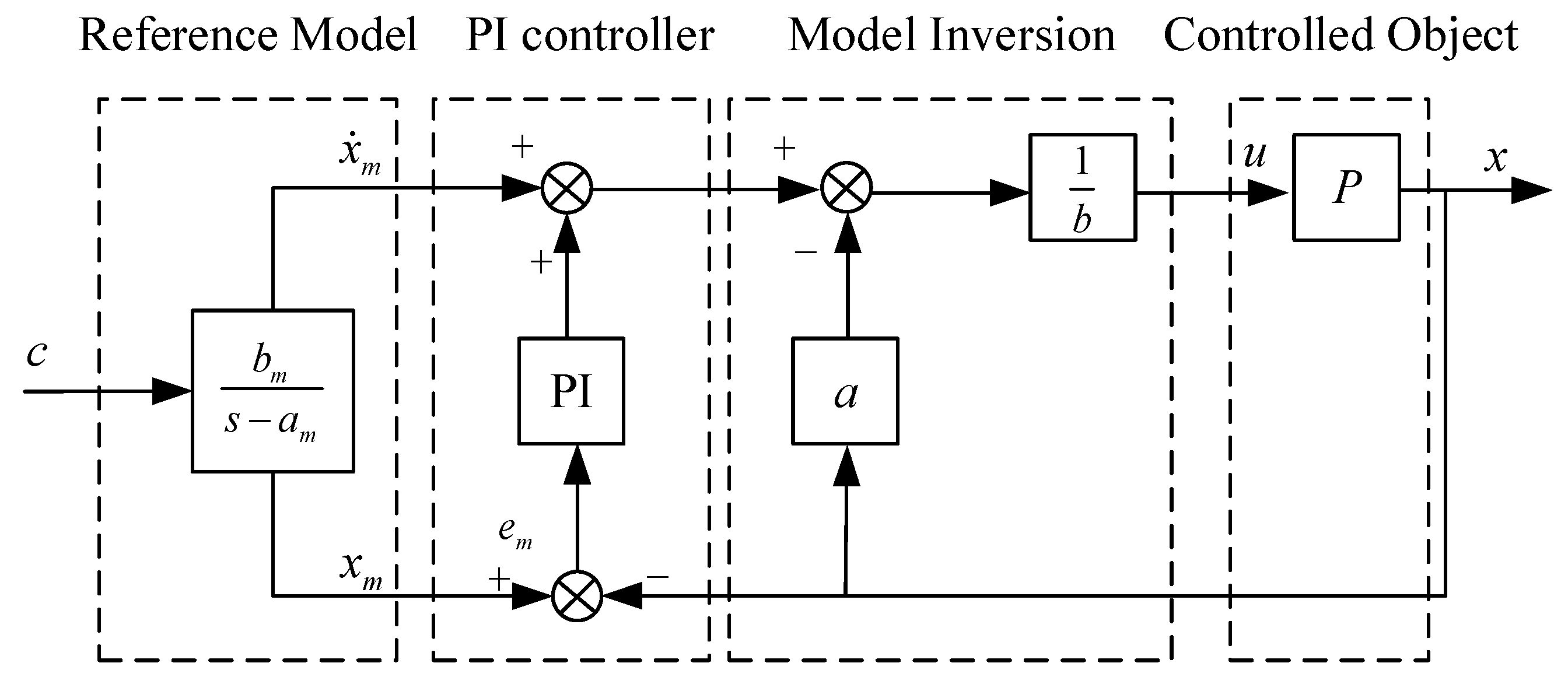
where K p = a m + k + β , K i = β ( a m + k ) . Its control structure is shown in Figure 1.
To analyze the system stability, define the following Lyapunov function:
V ( t ) = 1 2 e m 2 ( t )
Considering possible disturbances and potential signal distortion due to improper cutoff frequency selection of the low-pass filter, the filter error is defined as Δ u d t , according to the equations:
Δ u d ( t ) = u d ( t ) u ^ ( t ) = [ x ˙ ( t ) a x ( t ) b u ( t ) ] [ 1 g f ( t ) ]
From Figure 1, the error equation of the UDE control system is:
e ˙ m ( t ) = ( a m + k ) e m t Δ u d ( t )
Substituting the equation into the Lyapunov function and taking the derivative yields:
V ˙ ( t ) = e m ( t ) e ˙ m ( t ) = ( a m + k ) e m 2 ( t ) e m ( t ) Δ u d ( t )
According to Young’s inequality:
V t ( a m + k ) e m 2 ( t ) + 1 2 e m 2 ( t ) + 1 2 Δ u d 2 ( t ) c 1 V t + c 2
where c 1 = 2 ( a m + k ) 1 , c 2 is the upper bound of 1 2 Δ u d 2 ( t ) , and c 2 0 . When k = 0 , it can be ensured that c 1 > 0 . Solving this equation yields:
0 V ( t ) V ( 0 ) e m c 1 t + c 2 c 1 ( 1 e m c 1 t )
where V ( 0 ) = e m 2 ( 0 ) / 2 ; when t tends to positive infinity, e m c 1 t tends to 0, and c 2 / c 1 has an upper bound; therefore, the closed-loop system is also bounded.

2.2. Design of the UDE-Based PMSM Speed Loop Controller

Substituting the q-axis current reference value output by the controller into the mechanical equation yields:
J d ω ( t ) d t = K t i q * ( t ) T L B ω ( t )
In the equation, T L and B ω ( t ) are also considered as part of the disturbance. Let ω ( t ) be the system state value x ( t ) and i q * ( t ) be the control input u ( t ) . Then:
x ˙ ( t ) = b u ( t ) + d ( t )
where b = K t J , d ( t ) = 1 J [ B ω ( t ) T L ] , x ( t ) = ω ( t ) , u ( t ) = i q * ( t ) . According to the equation, let the parameter in the reference system a m = b m = α s , then:
x ˙ m ( t ) = α s x m ( t ) + α s c ( t )
where c ( t ) represents the speed input command ω * and x m ( t ) is the speed of the reference model ω m . Taking the Laplace transform of the equation:
s X m ( s ) = α s X m ( s ) + α s C ( s )
Rearranging the above equation:
G s ( s ) = α s s + α s
where α s represents the bandwidth value of the reference system. From the equation, design a first-order low-pass filter with bandwidth β s as follows:
G f s ( s ) = β s s + β s
Combining the equations, substituting into the equation, and setting k to zero yields the control law for the motor speed loop:
u ( t ) = 1 b x ˙ m ( t ) + K p e m ( t ) + K i 0 t e m ( τ ) d τ   = 1 b α s x m ( t ) + α s c ( t ) + K p e m ( t ) + K i 0 t e m ( τ ) d τ
where the values of the PI controller K p and K i are:
K p = α s + β s K i = α s β s
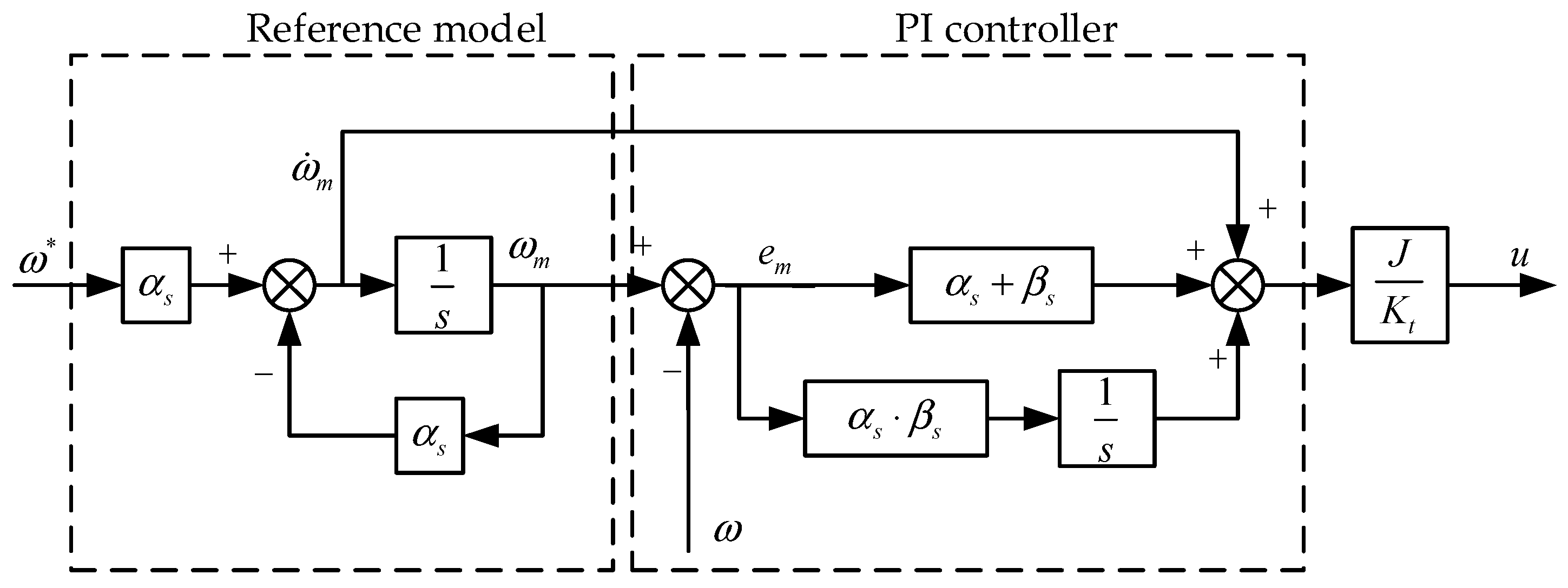
In summary, the derived UDE-based speed controller is shown in Figure 2. The proportional and integral gains of the speed loop control are both related to the desired reference system bandwidth α s and the lumped disturbance bandwidth β s . Therefore, the controller parameters are straightforward to input and provide good speed tracking performance.
The mathematical relationship for the PI controller’s proportional and integral gains is shown in the equation, with their values determined by α s and β s . Therefore, by controlling variables, one can first debug one value, observe the difference between the given signal and the feedback signal, and then debug the other value. The specific approach is as follows:
(1)
First, set the initial values of α s and β s
(2)
After debugging, fix the value of α s , then based on the feedback error, debug the value of β s . Generally, adjust β s from small to large until the feedback error approaches zero.
(3)
If the system bandwidth α s is set too large, it may lead to an inability to achieve ideal tracking performance even when increasing β s . Therefore, it is necessary to adjust c ( t ) according to the input speed command α s , and then follow step (2) to adjust β s

3. Application Research of Anti-Windup Algorithm in UDE Controller

In the UDE controller, integral action accumulation easily causes the Windup phenomenon under saturation. To address this, two anti-windup algorithms are introduced: piecewise tracking back-calculation and integral final value prediction. A symmetric anti-saturation compensation mechanism is constructed, and the two algorithms are compared to select the one more suitable for the UDE structure. This improvement effectively enhances the system’s dynamic response and control accuracy.

3.1. Windup Phenomenon in UDE Controller

In practical applications, controller outputs are constrained by physical limits, necessitating limiters that can induce windup. Saturation nonlinearity disrupts the symmetry of the control system, impairing closed-loop dynamics.
Under large step inputs, the integral term in the speed-loop UDE controller accumulates continuously while compensating for steady-state error, resulting in significant overshoot and oscillation. Once the current command exceeds the saturation limit, the system enters a nonlinear region with slowed response. The integrator continues to operate, and the high integral gain of UDE exacerbates response distortion.
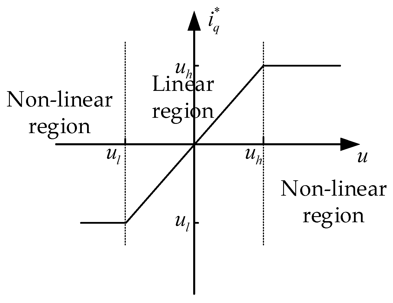
Figure 3 illustrates the saturation function. In this nonlinear region, system behavior deviates from the linear response, leading to prolonged settling time and possible sustained oscillations.
The Windup phenomenon causes the system output to fail to accurately track the reference input and may induce sustained oscillations, seriously affecting the reliability of industrial applications. Through a symmetrical compensation mechanism, performance degradation caused by saturation can be effectively suppressed without changing the original linear controller structure.
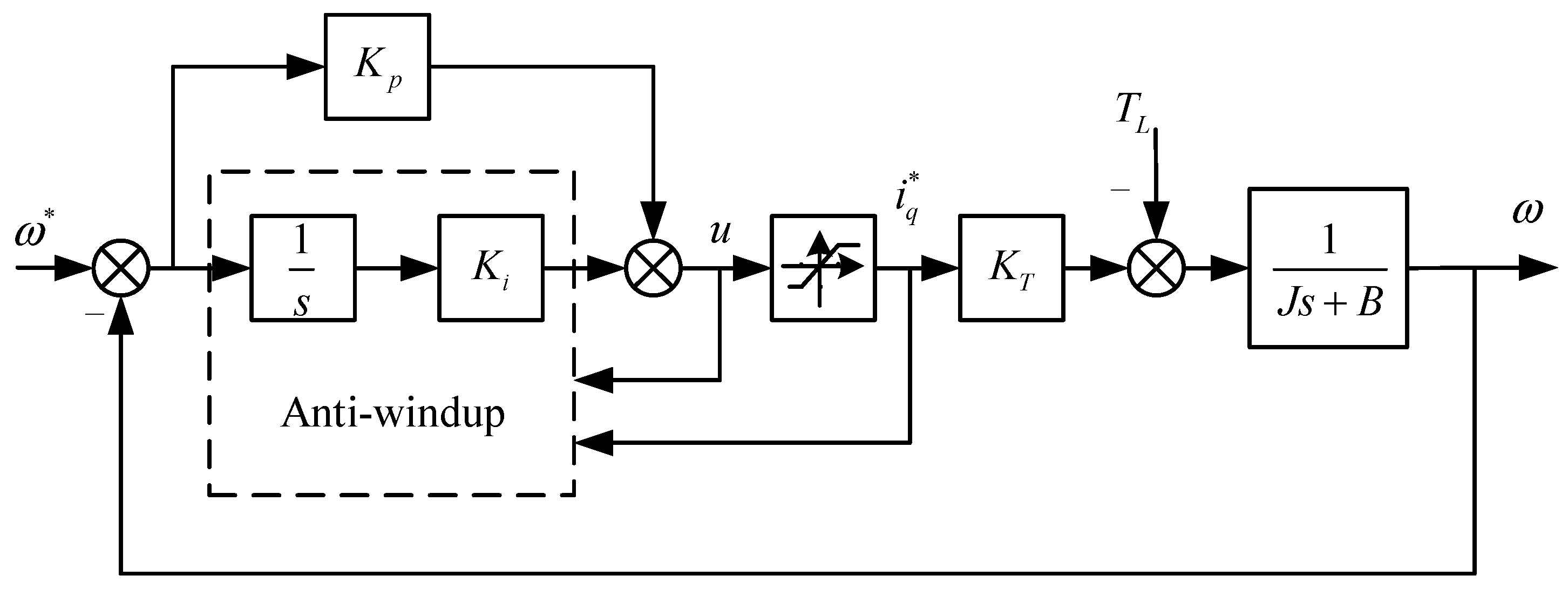
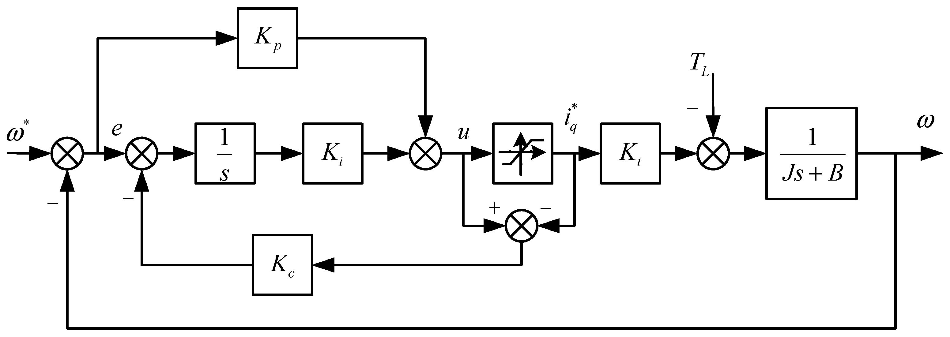
Figure 4 is the block diagram of the PMSM speed loop structure using a PI controller.
Under ideal conditions, without considering the windup link, the output of the speed loop PI controller is as follows.
u = e ( K p + K i s + K d s ) ( u i q * ) K c K i s   = e ( K p + K d s ) K i s [ e K c ( u i q * ) ]
where K c is the back-calculation coefficient; K p is the proportional gain; K i is the integral gain; K d is the derivative gain, generally 0 for speed loop controllers; u is the controller output signal.
The anti-windup algorithm prevents the excessive accumulation of the integral term during saturation. This enables a faster recovery of normal controller response, which improves dynamic performance by reducing overshoot and oscillation, enhancing stability, and shortening the settling time. The corresponding control block diagram is shown in Figure 5.
When the Anti-windup controller is in the linear region, its control method is essentially a PI controller, performing linear regulation on the system. When the controller enters the windup state, its mechanism involves defining a saturation depth u i q * and inputting K c into the integrator to achieve saturation control of the system. It should be noted that an increase in saturation depth makes the back-calculation effect more significant. Even when the saturation depth meets the condition of the equation, the integrator begins to accumulate in the opposite direction, even if the speed has not reached the set value. Therefore, adjusting the saturation depth and the proportional parameter K c becomes a key factor affecting the performance of the Anti-windup controller, directly related to the effectiveness of system saturation control and the optimization of overall performance.
u i q > | e | K c
The traditional tracking back-calculation anti-windup algorithm has a key limitation: its fixed back-calculation coefficient cannot adapt to varying operating conditions. While increasing this coefficient may reduce saturation depth, its effectiveness is interdependent with other parameters, making it insufficient for general application.

3.2. Research on Piecewise Tracking Back-Calculation Anti-Windup Algorithm

3.2.1. Algorithm Principle

The conventional tracking back-calculation method uses a fixed back-calculation coefficient K c , which lacks adaptability under varying saturation depths. To improve flexibility, a piecewise strategy is proposed, where K c is adjusted according to the saturation depth stage, enabling symmetric saturation compensation.
From the equation:
K c = e u i q *
When K c satisfies this equation, the value of the integrator is zero, which can be considered as the controller reaching saturation state, and the accumulated value of the integrator remains unchanged.
Under a large step signal, the proportional part responds rapidly to changes, while the integral action supplements it by eliminating steady-state error, thereby optimizing control performance. To prevent jitter near the saturation boundary due to disturbances, an error band with threshold b can be defined.
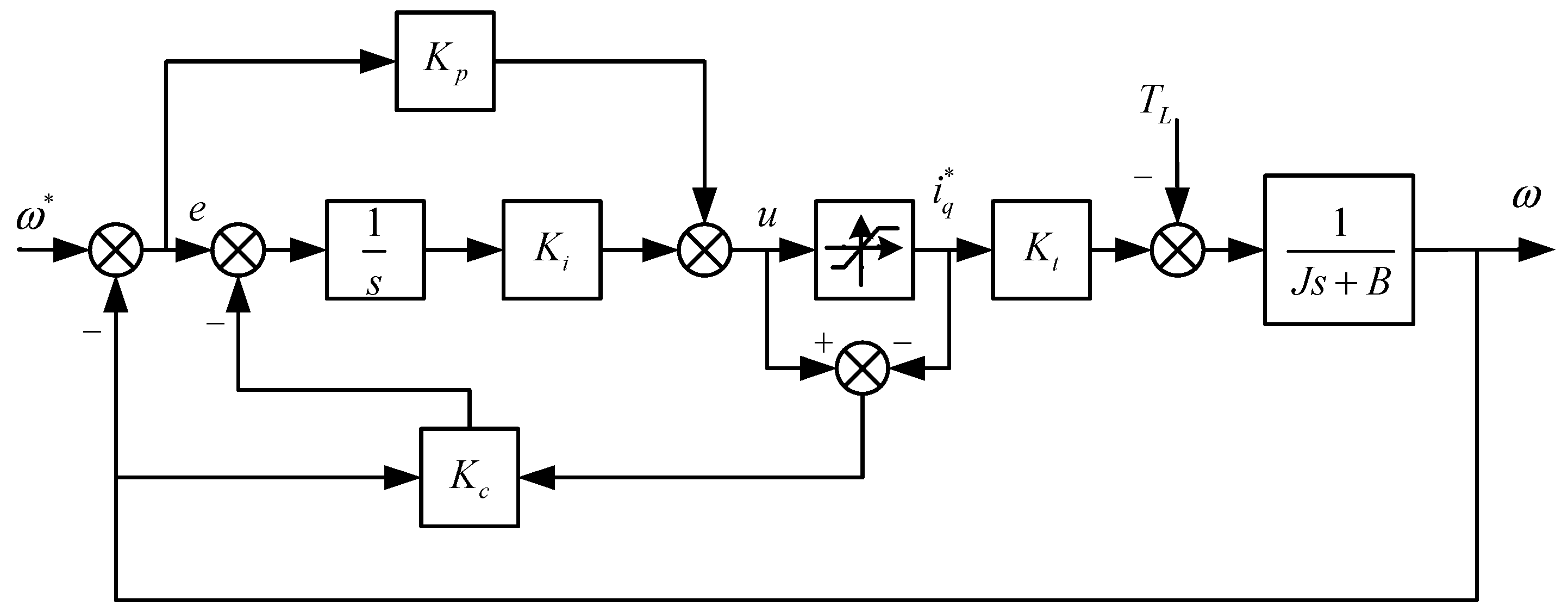
The value of the back-calculation coefficient K c corresponding to the critical region of system output saturation should be improved as:
K c = K c 0 ,   u i q * b e u i q * ,   u i q * > b
The back-calculation coefficient in the piecewise anti-windup regulator adjusts nonlinearly based on system operating stages such as startup, normal operation and load mutation. This enables the controller to flexibly counteract integral saturation under varying conditions, thereby improving system response, stability and drive performance.
The block diagram of the piecewise tracking back-calculation Anti-windup control is shown in Figure 6. This algorithm uses three variables e, u and i q * to adjust the tracking back-calculation parameter K c . Combined with formula analysis, it is known that the saturation depth threshold b needs to be adjusted to further adjust the back-calculation coefficient K c .
The piecewise anti-windup integral algorithm has certain limitations in practical application. Compared with traditional algorithms, these optimized methods introduce more parameters that need adjustment, which undoubtedly increases the reliance on engineering practical experience during the debugging process. Another point to note is that when dealing with discrete controllers where the accumulated value has discontinuous changes, the adjusted effect of such algorithms does not always meet expectations, which largely restricts the potential of the algorithm in practical applications.

3.2.2. Application Research in UDE Controller

The UDE controller with piecewise anti-windup is formulated as:
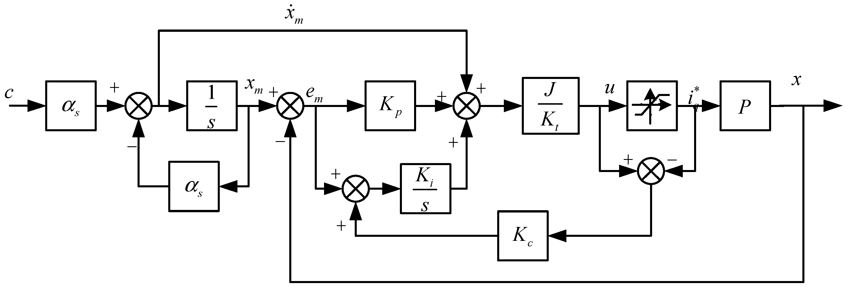
u ( t ) = 1 b x ˙ m + K p e m ( t ) + K i 0 t e m ( τ ) K a u ( τ ) i q * ( τ ) d τ
where e m ( t ) is the deviation between the desired reference system speed and the output speed. The control block diagram of the piecewise tracking back-calculation Anti-windup algorithm UDE controller is shown in Figure 7.
Based on the principle of piecewise back-calculation anti-windup, this strategy adds a logical judgment module to the control algorithm. It monitors whether the UDE output reaches saturation. The value of parameter K c is adjusted accordingly: maintaining its normal expression when unsaturated, and changing it once saturation occurs. This method confines the controller’s output within a permissible range. During normal unsaturated operation, the controller functions as designed. Upon saturation, the piecewise back-calculation mechanism activates to reduce or halt the accumulation of the integral term. This prevents the adverse effects of unexecuted control commands, significantly shortening the system’s recovery time and avoiding unnecessary overshoot. By leveraging the desaturation capability of traditional tracking back-calculation while improving its adaptability across various operating conditions, this approach optimizes overall control performance.

3.2.3. Simulation Analysis

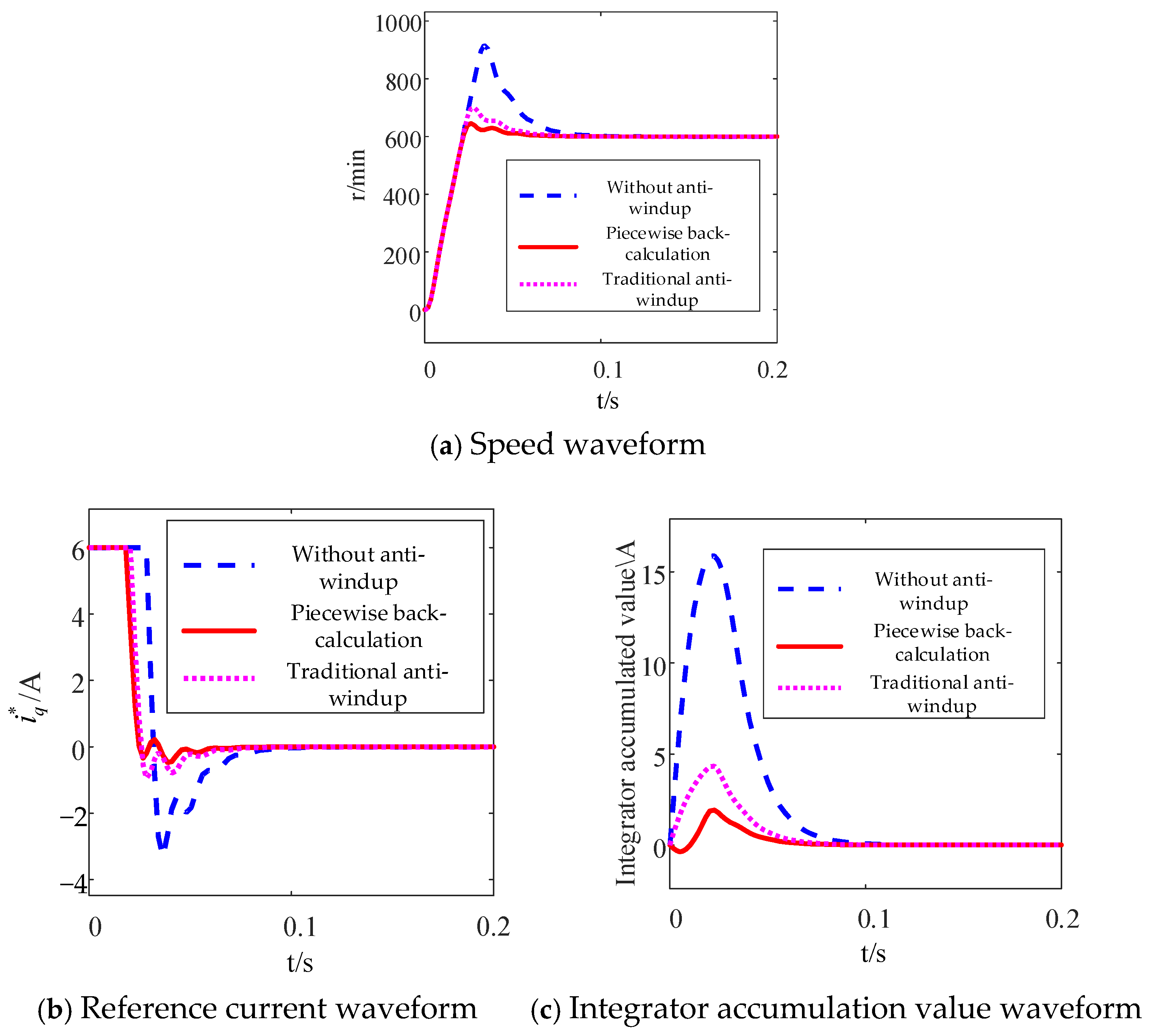
To demonstrate the improvements of the piecewise tracking back-calculation Anti-windup over the traditional tracking back-calculation Anti-windup, the following configurations were made for the two methods: In the tracking back-calculation Anti-windup, K c was fixed at 2.5; in the piecewise tracking back-calculation Anti-windup, the value of K c was the same, and the error band was selected as 1.5 times the current limit value, i.e., a = 9 . The simulation diagram of the piecewise tracking back-calculation Anti-windup is shown in Figure 8.
The piecewise tracking back-calculation anti-windup algorithm reduces the speed convergence time from 82.4 ms to 65.1 ms and the overshoot from 16.5% to 6.1% in the UDE controller, compared to the traditional method. This improvement is achieved through more intelligent integral saturation handling, which curbs integrator accumulation to lower overshoot and accelerate set-point tracking.

3.3. Research on Integral Final Value Prediction Anti-Windup Algorithm

3.3.1. Principle of Integral Final Value Prediction Anti-Windup Algorithm

The integral final value prediction Anti-windup algorithm is fundamentally a specific type of conditional integration method. Its core idea is to predict the final value of the integrator when the system reaches steady state through a symmetrical prediction mechanism, and adjust the integrator state accordingly to avoid excessive accumulation during saturation.
In the linear region, the controller expression can be represented as:
u ( t ) = K p e ( t ) + K i h ( t )
Define h ( t ) as the state of the integrator.
h ( t ) = 0 t e ( τ ) d τ
Substituting the equation into the PMSM mechanical equation yields:
e ˙ ( t ) = B J ω ( t ) K t J [ K p e ( t ) + K i h ( t ) ] + T L J
When the system is in steady state, ω = ω * and e ˙ = e = 0 , substituting into the equation, yields the integrator value at steady state:
h s s = B ω * + T L K t K i
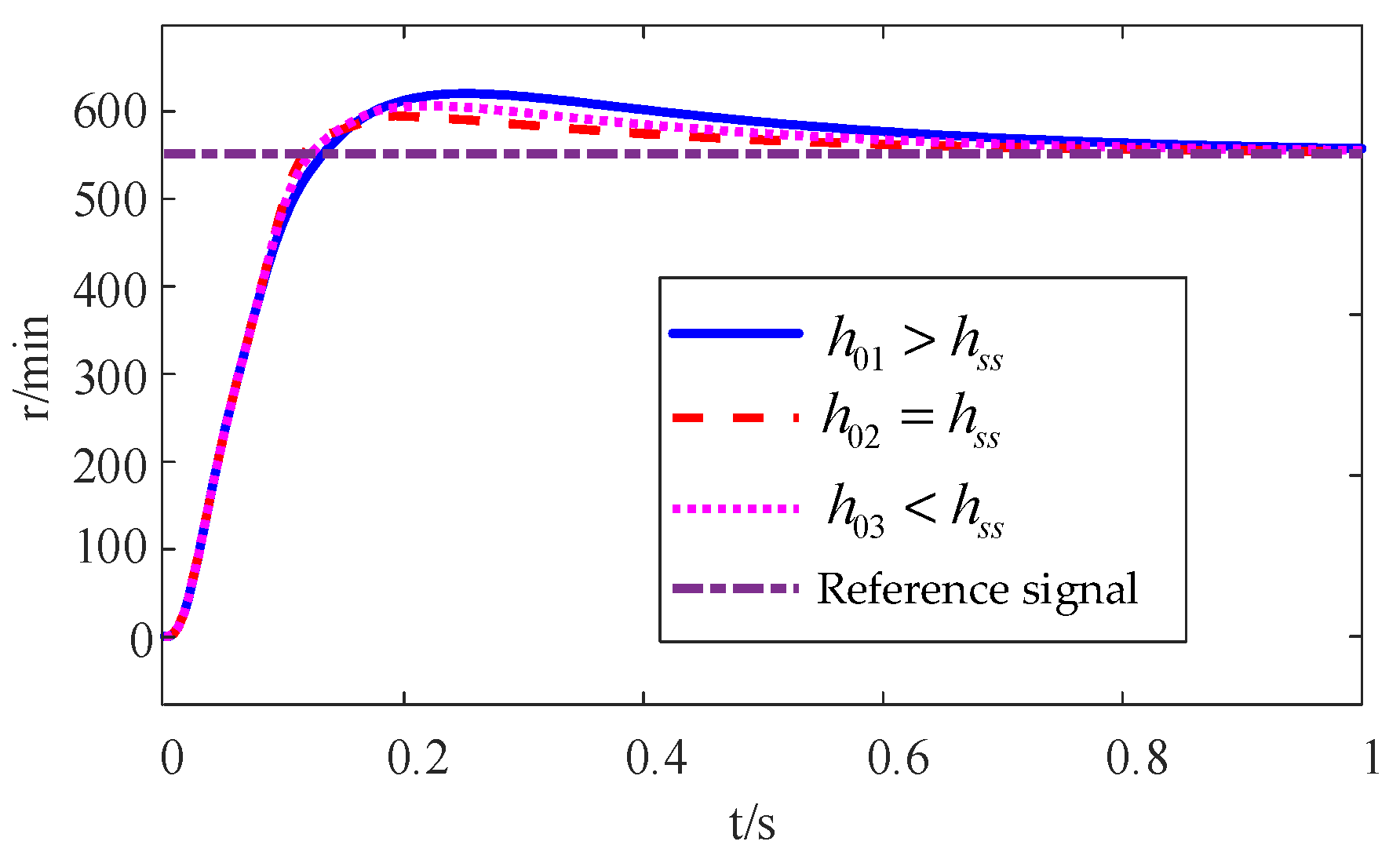
The stability of the control system is determined by the parameters of the PI controller. From Figure 9, it can be seen that when the PI controller operates in the linear region, different steady-state values of the integrator lead to different closed-loop system performances, including differences in overshoot, settling time, and steady-state error.
Rewrite the equation in the following form:
h ˙ = 1 τ h ( h ^ s s h ) u i q * ( Non linear   region ) e u = i q * ( Linear   region )
where h ^ s s is the estimated value of the integral state, τ h is the time constant of the filter, and its bandwidth is ω h . When the system is in the nonlinear region, then,
h ( s ) h s s ( s ) = 1 τ h s + 1 = ω h s + ω h
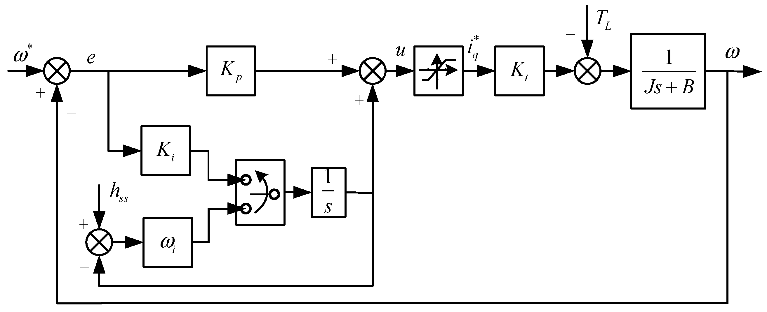
Figure 10 illustrates a PI controller equipped with integral final value prediction anti-windup. Within the linear region, the controller operates as a standard PI regulator without activating the anti-windup function, ensuring continuous output based on real-time error feedback. Once the output approaches or enters the nonlinear saturation region, the algorithm adjusts the integral term’s accumulation toward a predicted steady-state value. This adjustment, derived from the system dynamic model and output prediction, prevents the integrator from driving the output beyond physical limits due to sustained error buildup.

3.3.2. Application of Integral Final Value Prediction Anti-Windup Algorithm in UDE Controller

According to:
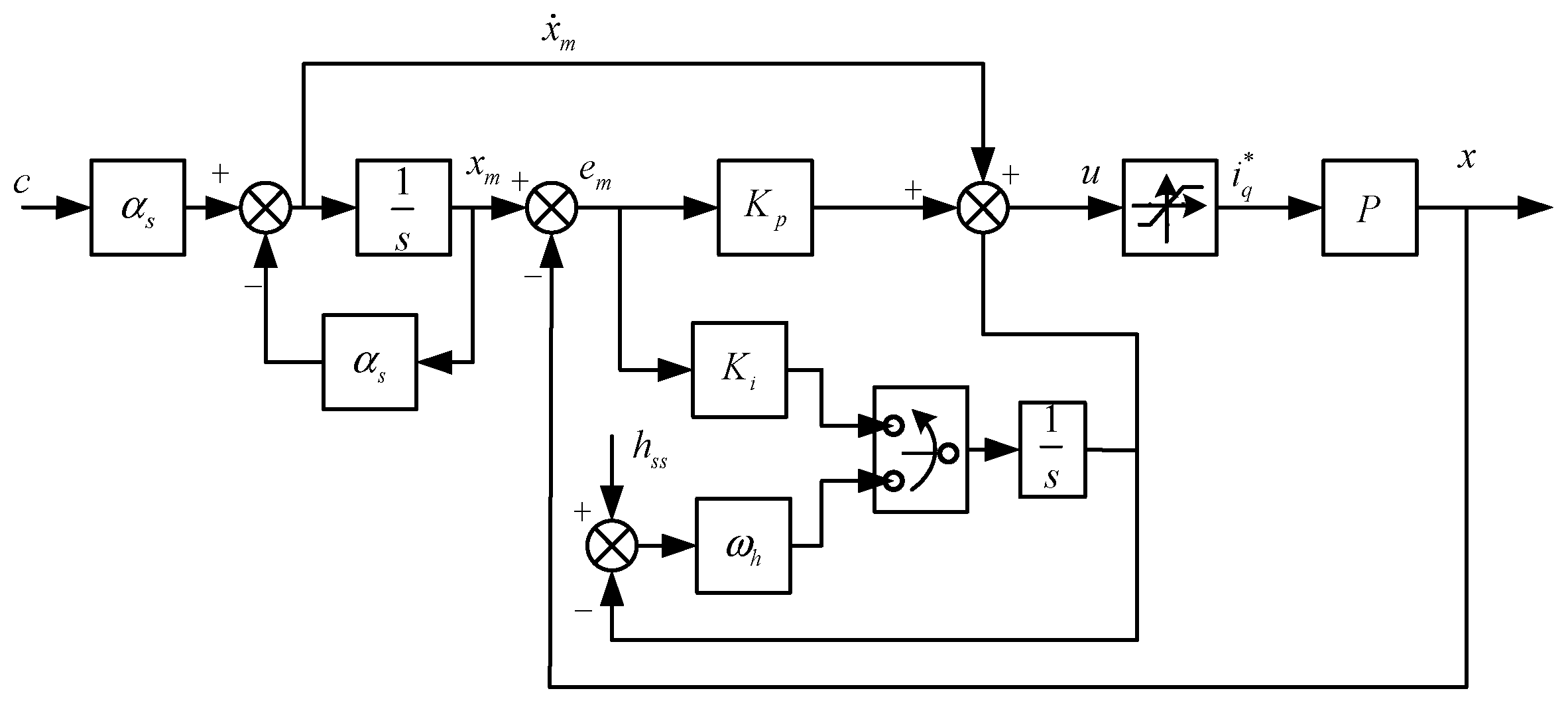
u ( t ) = 1 b [ x ˙ m ( t ) + K p e m ( t ) + K i q ( t ) ]
Substituting into yields:
x ˙ ( t ) = x ˙ m ( t ) + K p e m ( t ) + K i 0 t e m ( τ ) d τ + d ( t )
The adjusted state error dynamic equation is expressed as:
e ˙ m ( t ) = [ K p e m + K i q ( t ) + d ( t ) ]
From the equations, the steady-state value of the integrator is obtained through calculation:
h s s = d s s K i = B ω * + T L K i J
From the equation, it can be seen that the integrator steady-state value h s s is related to the speed reference, controller bandwidth, load torque, and viscous friction coefficient.
Take a speed mutation process as an example. This process includes the saturated part of the controller output, assuming it occurs within the time interval from t = 0 to t 2 . In this case, time t 1 is the critical point between the saturation region and the linear region. Further analysis is conducted below.
Given that the viscous friction coefficient B is very small and the load torque T L is regarded as constant, the combined effect of the viscous friction term and the load torque T L can be collectively treated as a disturbance term d ( t ) = d s s . Substituting into the equation yields:
e ˙ m ( t ) = K p e m ( t ) K i [ h ( t ) h s s ]
Performing differential processing on the error equation e m ( t ) = x m ( t ) x ( t ) and applying the Laplace transform to the resulting differential equation yields:
s E m ( s ) e m ( 0 ) = [ s X m ( s ) x m ( 0 ) ] [ x X ( s ) x ( 0 ) ]
Set the initial value of the equation as:
x ( 0 ) = x m ( 0 ) = ω 0 e m ( 0 ) = ω 0 ω *
When the controller is saturated, the output is u s and its value range is u s = i q max * , i q min * , then:
d x d t = K t u s T L J = k s
Therefore, it can be understood that the motor speed exhibits linear change in the saturation region, with its change slope denoted as k s . Thus, the speed formula in the corresponding saturation region can be expressed as:
x ( t ) = k s t + ω 0
where the value range of t is 0 , t 1 . Therefore, the desired reference system speed can be calculated as:
x m ( t ) = ( ω * ω 0 ) ( 1 e m α s t ) + ω 0
Combining the equations, the error equation between the reference model and the actual system model is obtained:
e m ( t ) = x m ( t ) x ( t ) = ( ω * ω 0 ) ( 1 e m α s t ) k s t
If for given parameters, the critical time moment t 1 between the saturation region and the linear region is fixed, then the error e m ( t 1 ) at this moment can be regarded as a fixed value.
When the system enters the nonlinear region, perform Laplace transform on the formula; the result is as follows:
s E m ( s ) e m ( t 1 ) = K p E m ( s ) K i E m ( s ) + h ( t 1 ) s h s s s
In this formula, h ( t 1 ) is the initial value of the integrator when entering the nonlinear region. By organizing the formula, the error dynamic response of the actual system relative to the expected reference system can be obtained as:
E m ( s ) = s s 2 + K p s + K i e m ( t 1 ) + K i s 2 + K p s + K i [ h s s h ( t 1 ) ]
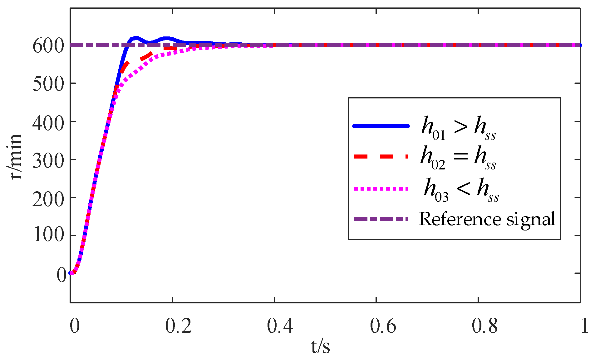
The relationship between the integrator steady-state value and the dynamic response of the speed loop controller output is shown in Figure 11.
From Figure 11, it can be seen that the UDE-based speed loop controller and the PI controller are consistent in their dynamic performance relationship with the integrator initial value. Based on this, the control equation for the saturation region is:
u ( t ) = 1 b [ x ˙ m ( t ) + K p e m ( t ) + h ( t ) ] h ˙ ( t ) = ω i [ h ^ s s h ( t ) ]
For the critical moment t = t 1 between the saturation region and the non-saturation region, substituting the equation into the equation yields:
b u s = α s ( ω * ω 0 ) e m α s t 1 + K p [ ( ω * ω 0 ) ( 1 e m α s t 1 ) k s t ] + h s s ( 1 e m ω i t 1 )
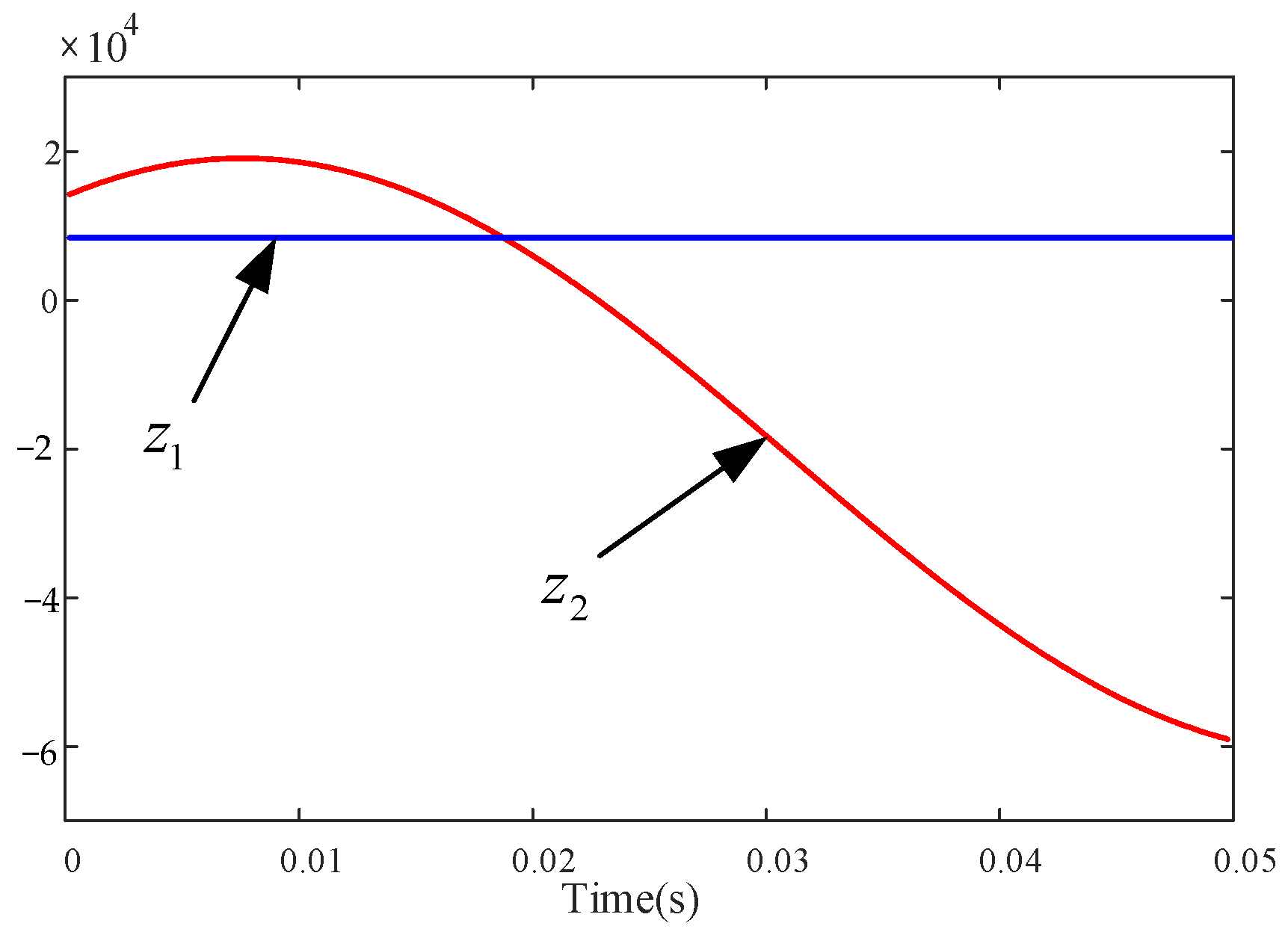
In this formula, there is only one unknown number t 1 . Next, use the graphical solution method to solve for the numerical value of t 1 .
Define the left side of the equation as z 1 , and the right side as z 1 , as shown in Figure 12.
From Figure 12, the value of t 1 can be found using the graphical solution method. Thus, any parameter required for the integral final value prediction Anti-windup algorithm can be calculated.
The integral state prediction anti-windup algorithm addresses the UDE controller’s integral saturation issue by predicting the integrator’s steady-state value. When the controller output saturates, this predicted value is preset as the initial integral state upon returning to the linear region. A low-pass filter with suitable bandwidth is applied to ensure prediction accuracy by attenuating high-frequency disturbances. This approach effectively mitigates the overshoot and extended settling time induced by integral saturation, thereby optimizing the control system’s response speed and stability. The structure is shown in Figure 13.

3.3.3. Simulation Analysis

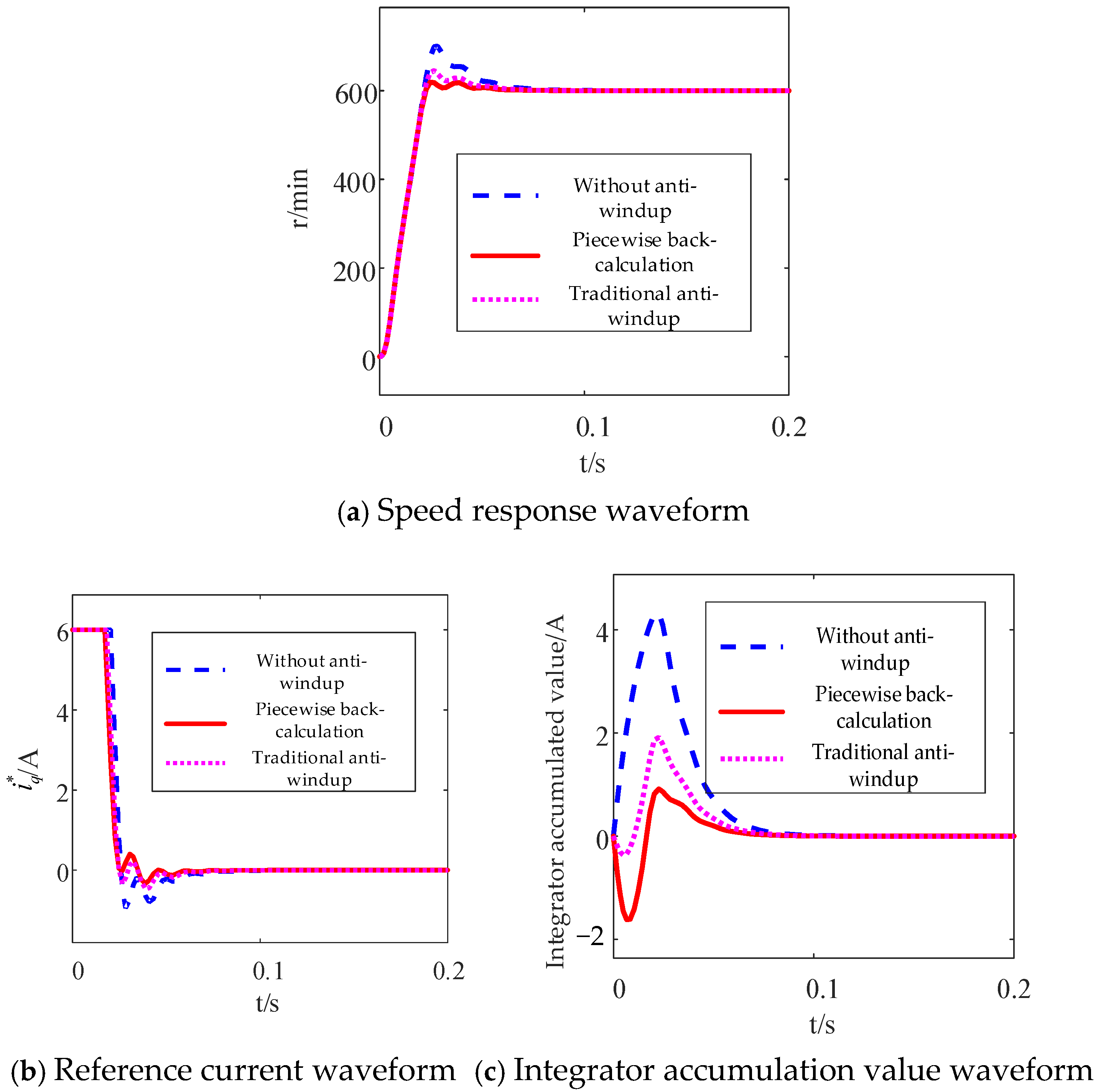
For the integral final value prediction Anti-windup algorithm, according to the formula, h s s = 828 , and the low-pass filter bandwidth value is 400. The simulation results are shown in Figure 14.
From Figure 14, the UDE controller with the integral final value prediction anti-windup algorithm achieves a convergence time of 58.7 ms and an overshoot of 4.3%, shortening convergence time by 6.3 ms and reducing overshoot by 1.8% compared to the piecewise tracking back-calculation anti-windup algorithm. The data shows the traditional tracking back-calculation anti-windup algorithm is a special case of the integral final value prediction version (when the predicted steady-state value is less than the actual one and h s s = 0 ). By accurately estimating the steady-state value of h s s , the integral final value prediction algorithm avoids delaying the system’s exit from saturation and sets an appropriate initial integrator value in the linear region, enabling faster target tracking and better consistency between the speed feedback curve and the ideal control effect.

4. Experimental Setup

First, the hardware composition and software program of the experimental platform were designed, with corresponding hardware circuit diagrams and software flowcharts drawn. During the experiment, the proposed UDE controller was integrated with the piecewise tracking back-calculation anti-windup algorithm and the integral final value prediction anti-windup algorithm, respectively, and their performance was evaluated. Experiments verified that the integral final value prediction anti-windup algorithm can effectively optimize the overshoot of the UDE controller.

4.1. Experimental Verification and Analysis

The piecewise tracking back-calculation anti-windup algorithm in the UDE controller runs in the interrupt function. Its process involves comparing the PI controller’s output with the limited q-axis current reference value, judging oversaturation via the difference and saturation depth. If unsaturated, a fixed feedback coefficient is added to the integrator; if saturated, the back-calculation coefficient uses the traditional value when saturation depth is below the threshold, and the maximum coefficient when exceeding it, ensuring an appropriate feedback coefficient across states.
The integral final value prediction anti-windup algorithm differs in that it is inactive when unsaturated. When saturated, the integrator gain is the predicted steady-state value, derived from the calculated steady-state value processed by a low-pass filter.

4.2. Experimental Analysis of Anti-Windup Algorithm Application in UDE Controller

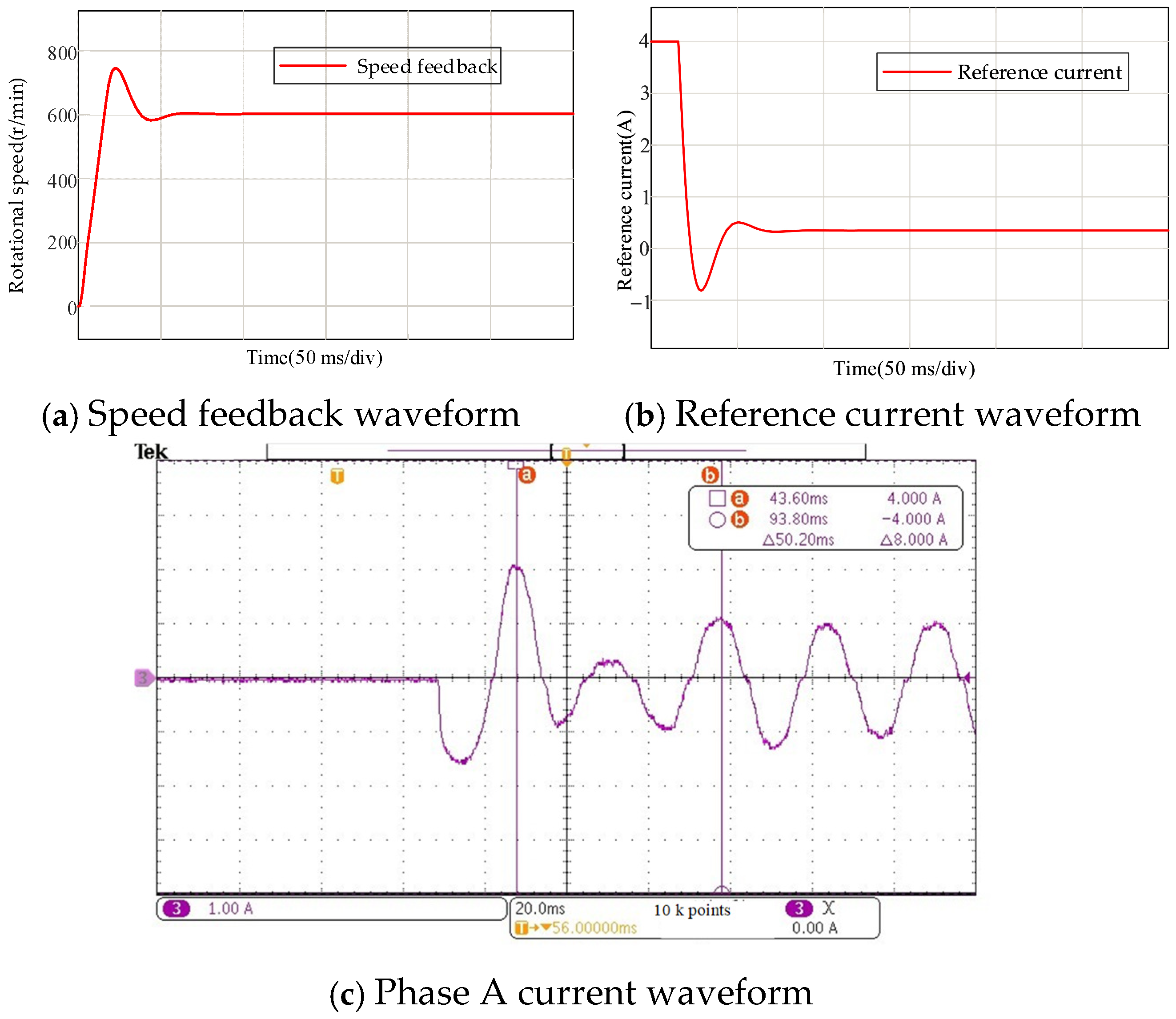
To verify the effectiveness of the Anti-Windup algorithm in the UDE controller, the motor’s given speed was set to 600 r/min, and a load of 1 N·m was provided by the load motor. Meanwhile, the current output value limit was set within the range of ±4A. Experiments were conducted without the Anti-Windup algorithm, with the piecewise tracking back-calculation Anti-Windup algorithm, and with the integral final value prediction Anti-Windup algorithm, respectively. The experimental parameter table is shown in Table 1.
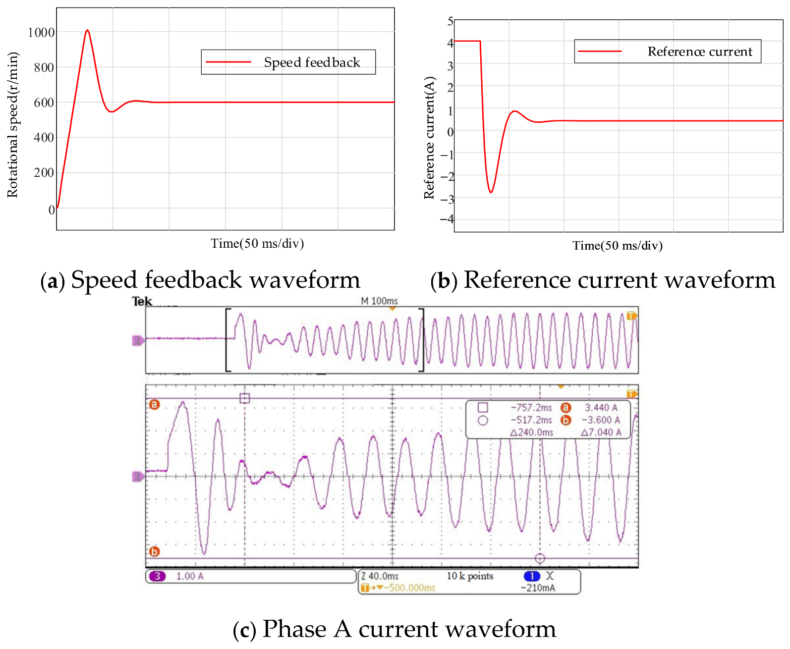
The experimental results without the Anti-Windup algorithm are shown in Figure 15.
From Figure 15, when no Anti-Windup algorithm is used, it can be observed that the overshoot of the speed feedback is about 66%, which significantly increases the system’s overshoot phenomenon. The excessive increase in overshoot not only affects the system’s stability, but also, from the fluctuation of the Phase A current, it can be seen that the excessive speed overshoot leads to significant fluctuations in the Phase A current in the initial stage of motor operation. Therefore, to reduce the speed overshoot and mitigate the Phase A current fluctuations, it is necessary to introduce an Anti-Windup algorithm into the control system to enhance system stability and improve dynamic response.
The experimental results of applying the piecewise tracking back-calculation Anti-Windup algorithm in the UDE controller are shown in Figure 16.
From Figure 16, when the system adopts the piecewise tracking back-calculation Anti-Windup algorithm, the speed feedback overshoot is about 34%. Compared with when no Anti-Windup algorithm is used, the speed feedback overshoot of this algorithm is reduced by 22%, significantly reducing the system’s overshoot phenomenon. Moreover, from the Phase A current waveform, it can be seen that it only shows large current fluctuations in the first cycle. At the same time, the response speed of the system feedback speed is faster. Adopting this algorithm not only optimizes the dynamic performance of the system but also improves the efficiency of speed control, reduces adverse impacts on the motor, thereby further improving the stability and reliability of the entire control system.
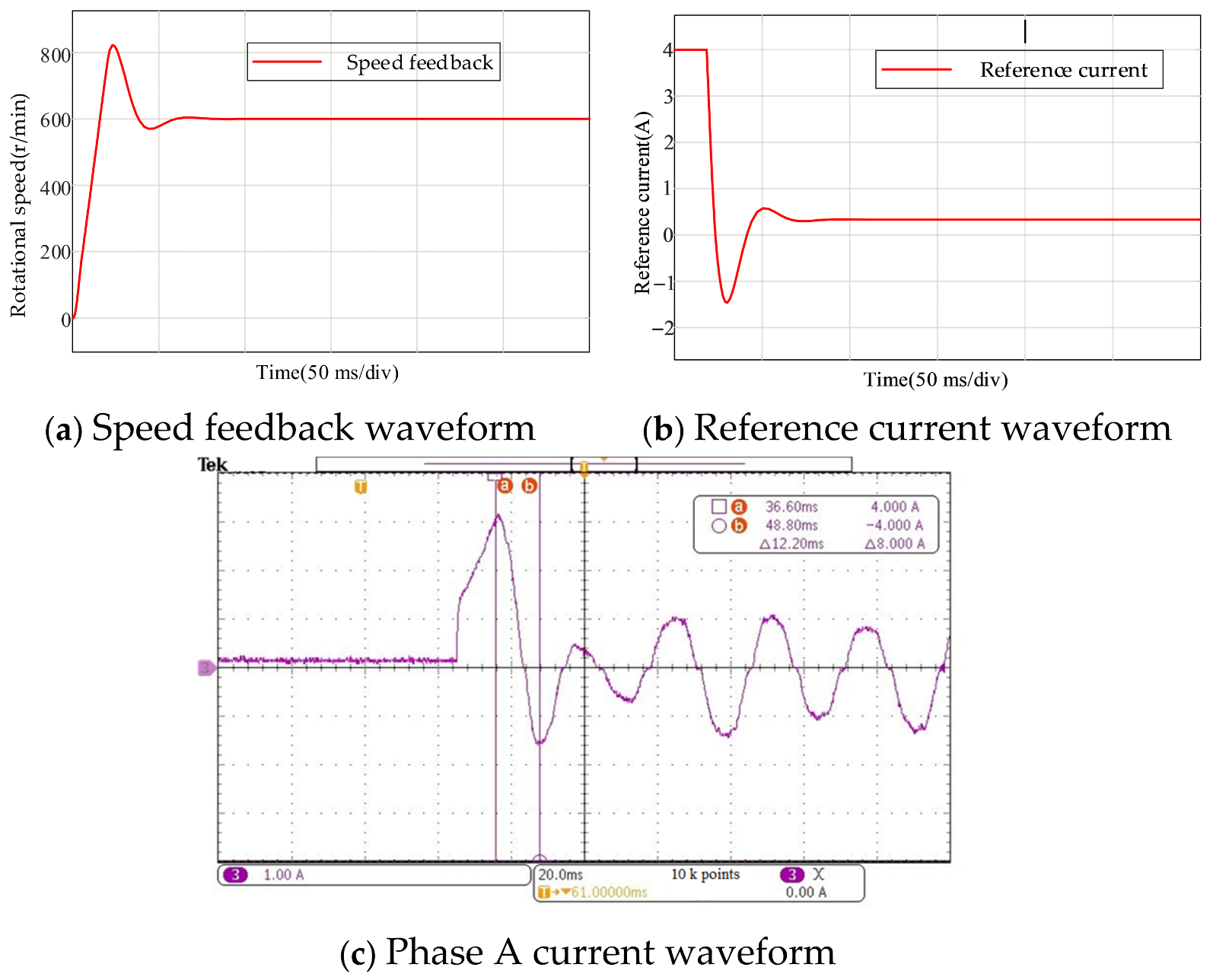
The experimental results of applying the integral final value prediction Anti-Windup algorithm in the UDE controller are shown in Figure 17.
From Figure 17, when the system adopts the integral final value prediction Anti-Windup algorithm, the speed feedback overshoot is about 19%. Compared with when using the piecewise tracking back-calculation Anti-Windup algorithm, the speed feedback overshoot of this algorithm is reduced by 15%, significantly reducing the system’s overshoot phenomenon. Moreover, from the Phase A current waveform, it can be seen that the current fluctuation in the first cycle is also significantly reduced compared to the piecewise tracking back-calculation Anti-Windup algorithm. In addition, the system’s feedback response speed is accelerated, indicating that the integral final value prediction Anti-Windup algorithm can effectively reduce the speed feedback overshoot and accelerate the system’s response to commands, thereby improving the overall control performance and dynamic response capability.

4.3. Chapter Summary

This chapter first designed the required hardware and software parts for the experiment. Then, experiments were conducted on the hardware platform designed in this chapter for the speed loop control strategy optimization algorithms proposed in this paper, and software programs were written for the aforementioned algorithms. The following conclusions can be drawn from the experiments:
Compared to when no Anti-Windup algorithm was used, the speed feedback overshoot of the UDE controller using the piecewise tracking back-calculation Anti-Windup algorithm is reduced by 22%; compared to when using the piecewise tracking back-calculation Anti-Windup algorithm, the speed feedback overshoot of the UDE controller using the integral final value prediction Anti-Windup algorithm is reduced by 15%. This proves that the algorithms proposed in this paper have a significant optimization effect on speed loop control, producing positive impacts in improving response speed, reducing overshoot, and enhancing system stability.

5. Conclusions

5.1. Full Text Summary

This paper mainly focuses on researching the improvement of the response problem of the speed loop controller in the vector control of Permanent Magnet Synchronous Motor (PMSM) servo systems. First, mathematical modeling of the PMSM current-speed double closed-loop system was performed, and parameter tuning calculations for its PI controller were conducted. This paper introduces a controller based on Uncertainty and Disturbance Estimation (UDE), defining the viscous friction coefficient and load torque as lumped disturbances to reduce their impact on the speed loop controller. Since the UDE controller suffers from severe Windup phenomenon, the integral final value prediction Anti-Windup algorithm was introduced, improving the system’s dynamic response. Finally, simulation comparison and experimental verification were carried out. The full text summary is as follows.
The Uncertainty and Disturbance Estimation control method was applied to the PMSM speed loop control, and parameter tuning calculation analysis was performed for this controller. The principle of the UDE controller was analyzed, and its stability was verified. To address the Windup problem existing in the UDE controller, two solutions were introduced: the piecewise tracking back-calculation Anti-Windup algorithm and the integral final value prediction Anti-Windup algorithm. Simulation experiments proved their effectiveness.
A servo system hardware platform based on the STM32F446 processor was built. Experiments were conducted on the UDE controller with the Anti-Windup algorithm in the speed loop control, proving the effectiveness of the algorithm.

5.2. Work Outlook

This paper conducted algorithm optimization and research to improve the response of the PMSM speed loop control system. Due to time constraints and limited knowledge, there are still many areas in this paper that need optimization and improvement. In future research, the following directions can be explored:
Currently, the integral steady-state value h s s for the integral final value prediction Anti-Windup algorithm is calculated only offline. However, this calculation method is not precise. Under different load conditions, h s s will change accordingly, which may reduce the system’s dynamic response. Therefore, in future research directions, solutions for obtaining h s s online can be explored.

Author Contributions

Conceptualization, H.S. (Hui Song) and S.L.; methodology, H.S. (Hui Song); software, H.S. (Hui Song); validation, H.S. (Haiyan Song); formal analysis, S.L.; investigation, H.S. (Haiyan Song); resources, S.L.; data curation, H.S. (Haiyan Song); writing—original draft preparation, H.S. (Hui Song); writing—review and editing, S.L.; visualization, Z.F.; supervision, Z.F.; project administration, H.S. (Haiyan Song); funding acquisition, H.S. (Hui Song). All authors have read and agreed to the published version of the manuscript.

Funding

Development Technology and Innovation of Amorphous Motors for Compressors (KYH2024186).

Data Availability Statement

The original contributions presented in this study are included in the article. Further inquiries can be directed to the corresponding author.

Conflicts of Interest

The authors declare no conflicts of interest.

References

  1. Wang, Y. Bounded UDE-based robust control for MIMO systems with application to vector control of a PMSM drive. TechRxiv 2023. [Google Scholar] [CrossRef] [Scilit]
  2. Milanowski, H.; Piłat, A.K. Neural Flux-Domain Encoder Resilient to Rotor Eccentricity in BLDC Drives. Sensors 2026, 26, 50. [Google Scholar] [CrossRef] [Scilit]
  3. Yang, Z.; Zhu, W.; Zhi, P. A Novel Adaptive RNN-Based Control Strategy for Deep Flux-Weakening Operation of IPMSMs. Electronics 2025, 14, 4934. [Google Scholar] [CrossRef] [Scilit]
  4. Oldoini, D.; Barbieri, S.G.; Devito, G.; Giacopini, M.; Galea, M. Effects of an Optimized Adhesive Distribution on Stresses and Strains in the Rotor and Magnets of a Surface Permanent-Magnet Synchronous Electric Motor. Appl. Sci. 2025, 15, 13179. [Google Scholar] [CrossRef] [Scilit]
  5. Zhou, X.; Guan, X.; Liu, X.; Zhao, R. Model Predictive Control Strategy for Open-Winding Motor System Based on ResNet. Symmetry 2025, 17, 2146. [Google Scholar] [CrossRef] [Scilit]
  6. Sapmaz, T.; Bakan, A.F. Experimental Evaluation of Pulsating and Rotating HFI Methods with Adaptive-Gain SMO for Sensorless IPM Compressor Drives. World Electr. Veh. J. 2025, 16, 669. [Google Scholar] [CrossRef] [Scilit]
  7. Bai, J.; Zhang, L.; Xu, Y. Analysis on the Air-Gap Magnetic Field and Force of the Linear Synchronous Motor with Different Winding Distribution. Micromachines 2025, 16, 1396. [Google Scholar] [CrossRef] [Scilit] [PubMed]
  8. Sun, X.; Yin, H.; Chen, Y.; Luo, M.; Wang, X.; Hu, W. Research on Active Disturbance Rejection-Based Control Technology for Agricultural Permanent Magnet Synchronous Motors. Agriculture 2025, 15, 2553. [Google Scholar] [CrossRef] [Scilit]
  9. Zhao, K.; Yin, T.; Zhang, C.; He, J.; Li, X.; Chen, Y. Robust model-free nonsingular terminal sliding mode control for PMSM demagnetization fault. IEEE Access 2019, 7, 15737–15748. [Google Scholar] [CrossRef] [Scilit]
  10. Junejo, A.K.; Xu, W.; Mu, C.; Ismail, M.M.; Liu, Y. Adaptive speed control of PMSM drive system based a new sliding-mode reaching law. IEEE Trans. Power Electron. 2020, 35, 12110–12121. [Google Scholar] [CrossRef] [Scilit]
  11. Liu, G.; Chen, B.; Wang, B.; Song, X. Selective current harmonic suppression for high-speed PMSM based on high-precision harmonic detection method. IEEE Trans. Ind. Inform. 2018, 15, 3457–3468. [Google Scholar] [CrossRef] [Scilit]
  12. Zhao, K.; Zhou, R.; She, J.; Zhang, C.; He, J.; Huang, G. Demagnetization-fault reconstruction and tolerant-control for PMSM using improved SMO-based equivalent-input-disturbance approach. IEEE/ASME Trans. Mechatron. 2021, 27, 701–712. [Google Scholar]
  13. Wang, Y.; Yang, M.; Wang, Y. Bounded UDE-Based Robust Control for MIMO Systems Based on a Nonlinear Design of Error Dynamics. IEEE J. Emerg. Sel. Top. Ind. Electron. 2025, 6, 1756–1765. [Google Scholar] [CrossRef] [Scilit]
  14. Gao, S.; Wei, Y.; Zhang, D.; Qi, H.; Wei, Y.; Yang, Z. Model-free hybrid parallel predictive speed control based on ultralocal model of PMSM for electric vehicles. IEEE Trans. Ind. Electron. 2022, 69, 9739–9748. [Google Scholar] [CrossRef] [Scilit]
  15. Sarsembayev, B.; Suleimenov, K.; Do, T.D. High order disturbance observer based PI-PI control system with tracking anti-windup technique for improvement of transient performance of PMSM. IEEE Access 2021, 9, 66323–66334. [Google Scholar] [CrossRef] [Scilit]
  16. Li, J.; Zhang, L.; Luo, L.; Li, S. Extended state observer based current-constrained controller for a PMSM system in presence of disturbances: Design, analysis and experiments. Control Eng. Pract. 2023, 132, 105412. [Google Scholar] [CrossRef] [Scilit]
  17. Zhang, Z.; Wang, Y.; Wang, C.; Su, Y.; Wang, Y.; Dai, Y. Distributed Chance-Constrained Optimal Dispatch for Integrated Energy System With Electro-Thermal Couple and Wind-Storage Coordination. IEEE Trans. Ind. Appl. 2025, 61, 833–846. [Google Scholar] [CrossRef] [Scilit]
Figure 1. Structural Block Diagram of UDE Controller.
Symmetry 18 00116 g001
Figure 2. Block diagram of the speed loop UDE controller principle structure.
Symmetry 18 00116 g002
Figure 3. Saturation function schematic.
Symmetry 18 00116 g003
Figure 4. Speed loop control model.
Symmetry 18 00116 g004
Figure 5. Tracking back-calculation Anti-windup control block diagram.
Symmetry 18 00116 g005
Figure 6. Piecewise tracking back-calculation Anti-windup control block diagram.
Symmetry 18 00116 g006
Figure 7. Block diagram of the piecewise tracking back-calculation Anti-windup algorithm UDE controller.
Symmetry 18 00116 g007
Figure 8. Piecewise tracking back-calculation Anti-windup simulation diagram.
Symmetry 18 00116 g008
Figure 9. Influence of different integrator initial values on control performance.
Symmetry 18 00116 g009
Figure 10. Integral state final value prediction Anti-Windup control block diagram.
Symmetry 18 00116 g010
Figure 11. Influence of the relationship between integrator steady-state value and initial value on output dynamics.
Symmetry 18 00116 g011
Figure 12. Schematic diagram of graphical solution for critical time.
Symmetry 18 00116 g012
Figure 13. Structure block diagram of the UDE controller with integral state prediction Anti-windup algorithm.
Symmetry 18 00116 g013
Figure 14. Integral final value prediction Anti-windup algorithm simulation diagram.
Symmetry 18 00116 g014
Figure 15. Experimental results of UDE controller without Anti-Windup algorithm.
Symmetry 18 00116 g015
Figure 16. Experimental results of piecewise tracking back-calculation application in UDE controller.
Symmetry 18 00116 g016
Figure 17. Experimental results of integral final value prediction application in UDE controller.
Symmetry 18 00116 g017
Table 1. Experimental parameter table.
ParameterValue
Rated Power/W750
Rated Line Voltage/V220
Rated Line Current/A4
Winding Inductance/H7
Winding Resistance/Ω3.2
Moment of Inertia/kg·m20.0004
Viscous Friction Coefficient/N·m·s0.001
Disclaimer/Publisher’s Note: The statements, opinions and data contained in all publications are solely those of the individual author(s) and contributor(s) and not of MDPI and/or the editor(s). MDPI and/or the editor(s) disclaim responsibility for any injury to people or property resulting from any ideas, methods, instructions or products referred to in the content.